Optimal Uncertainty Size in Distributionally Robust Inverse Covariance Estimation

Abstract

In a recent paper, Nguyen, Kuhn, and Esfahani (2018) built a distributionally robust estimator for the precision matrix of the Gaussian distribution. The distributional uncertainty size is a key ingredient in the construction of this estimator. We develop a statistical theory which shows how to optimally choose the uncertainty size to minimize the associated Stein loss. Surprisingly, rather than the expected canonical square-root scaling rate, the optimal uncertainty size scales linearly with the sample size.

1 Introduction

Motivated by a wide range of problems which require the estimation of the inverse of a covariance matrix, [9] recently constructed an estimator based on distributionally robust optimization using the Wasserstein distance in Euclidean space. A crucial ingredient is the distributional uncertainty size, which plays the role of a regularization parameter.

In their paper, [9] show excellent empirical performance of their estimator in comparison to several commonly used estimators (based on shrinkage and regularization). The comparison is based in terms of the corresponding Stein loss (defined in terms of the likelihood, as we shall review). However, no theory is provided as how to choose the distributional uncertainty size.

Our goal is to provide an asymptotically optimal expression for the distributional uncertainty size, in terms of the Stein loss performance, as the sample size increases.

This paper provides interesting insights which validate the empirical observations in [9]. In particular, in the Introduction of [9], leading to equation (4), they argue that the distributional uncertainty size, $\rho_{n}$, should scale at rate $\rho_{n}=O\left(n^{-1/2}\right)$ (where $n$ is the sample size) due to the existence of a central limit theorem for the Wasserstein distance for Gaussian distributions. However, the numerical experiments, reported in Section 6.1 of [9], suggest an optimal scaling of the form $\rho_{n}=O\left(n^{-\kappa}\right)$ where $\kappa>1/2$.

Our main result shows that the asymptotically optimal choice of distributional uncertainty is of the form $\rho_{n}=$ $\rho_{\ast}n^{-1}\left(1+o\left(1\right)\right)$ as $n\rightarrow\infty$, where $\rho_{\ast}>0$ is a constant which is characterized explicitly. Our results therefore validate the empirical findings of [9] with $\kappa=1$.

This paper is organized as follows. We review the estimator of [9] and state our main result in Section 2. We then provide the proof of our result in Section 3. Numerical experiments are included in Section 4, which provide a sense of the non-asymptotic performance of our asymptotically optimal choice.

2 Basic Notions and Main Result

We now review the basic definitions underlying the estimator from [9]. Suppose we have i.i.d. samples $\xi_{i}\sim\mathcal{N}\left(0,\Sigma_{0}\right)$ (normally distributed with zero mean and covariance matrix $\Sigma_{0}$), where $\xi_{i}\in\mathbb{R}^{d}$ and $\Sigma_{0}$ is assumed to be strictly positive definite. We write

$$\hat{\Sigma}_{n}=\frac{1}{n}\sum_{i=1}^{n}\xi_{i}\xi_{i}^{T},$$

and let $\mathbb{\hat{P}}_{n}$ correspond to a distribution with mean zero and covariance matrix $\hat{\Sigma}_{n}$, which we denote as $\mathcal{N}\left(0,\hat{\Sigma}_{n}\right)$. Throughout our development we use the notation $\left\langle A,B\right\rangle=$ tr$(A^{T}B)$ for any $d\times d$ matrices $A$, $B$, where $A^{T}$ denotes the transpose of $A$. The identity matrix is denoted by $I$. We use $\Rightarrow$ and $\overset{p}{\rightarrow}$ to denote weak convergence (convergence in distribution) and convergence in probability, respectively. Finally, for two symmetric matrices $A,B\in\mathbb{R}^{d\times d}$, $A\preceq B$ denotes that $A-B$ is positive semi-definite.

We define the Stein loss as

$$L(X,\Sigma_{0})=-\log\det(X\Sigma_{0})+\left\langle X,\Sigma_{0}\right\rangle-d,$$

where $X$ is any estimator of the precision matrix (i.e. the inverse covariance matrix).

Given an uncertainty size $\rho$, let us write $X_{n}^{\ast}(\rho)$ for the distributionally robust estimator proposed in [9]; i.e,

$$X_{n}^{\ast}(\rho)=\arg\min_{X\succ 0}\left\{-\log\det X+\sup_{\mathbb{Q}\in\mathcal{P}_{\rho}}\mathbb{E}^{\mathbb{Q}}\left[\left\langle\xi\xi^{T},X\right\rangle\right]\right\},$$ (1)

where $\mathcal{P}_{\rho}$ is the set of $d$-dimensional normal distributions with mean zero and which lie within distance $\rho$ measured in the Wasserstein sense, which we define next; see, for example, Chapter 7 in [11] for background on Wasserstein distances and, more generally, optimal transport costs. The Wasserstein distance (more precisely, the Wasserstein distance of order two with Euclidean norm) is defined as follows. First, let $\mathcal{M}_{+}(\mathbb{R}^{d}\times\mathbb{R}^{d})$ be the set of Borel (positive) measures on $\mathbb{R}^{d}\times\mathbb{R}^{d}$ and define the Wasserstein distance between $\mathbb{\hat{P}}_{n}$ and $\mathbb{Q}$ via

$$\mathbb{W}_{2}(\mathbb{\hat{P}}_{n},\mathbb{Q})=\inf_{\pi\in\mathcal{M}_{+}(\mathbb{R}^{d}\times\mathbb{R}^{d})}\left\{\left(\int\left\|z-w\right\|_{2}^{2}\pi\left(\mathrm{d}x,\mathrm{d}w\right)\right)^{1/2}\right.$$

$$:\int_{w\in\mathbb{R}^{d}}\pi\left(\mathrm{d}x,\mathrm{d}w\right)=\mathbb{\hat{P}}_{n}\left(\mathrm{d}x\right), \left.\int_{x\in\mathbb{R}^{d}}\pi\left(\mathrm{d}x,\mathrm{d}w\right)=\mathbb{Q}\left(\mathrm{d}w\right)\right\}.$$

Then

$$\mathcal{P}_{\rho}=\left\{\mathbb{Q}\sim\mathcal{N}\left(0,\Sigma\right)\text{ for some }\Sigma:\mathbb{W}_{2}(\mathbb{\hat{P}}_{n},\mathbb{Q})\leq\rho\right\}.$$

In simple terms, $\mathcal{P}_{\rho}$ is the set of probability measures corresponding to a Gaussian distribution which lie within $\rho$ units in the Wasserstein distance from $\mathbb{\hat{P}}_{n}$. It is well known (in fact, an immediate consequence of the delta method) that $n^{1/2}\mathbb{W}_{2}(\mathbb{\hat{P}}_{n},\mathbb{P}_{\infty})\Rightarrow\mathbb{W}$ for some limit law $\mathbb{W}$ which can be explicitly characterized (but not important for our development; see [10]). This result suggests that $\rho:=\rho_{n}$ should scale in order $O\left(n^{-1/2}\right)$. It is therefore somewhat surprising that the optimal scaling of $\rho$ for the purpose of minimizing the Stein loss is actually significantly smaller, as the main result of this paper indicates next.

Theorem 1.

Let

$$\rho_{n}=\arg\min_{\rho\geq 0}\{\mathbb{E}[L(X_{n}^{\ast}(\rho),\Sigma_{0})]\},$$ (2)

then

$$\lim_{n\rightarrow\infty}n\rho_{n}=\rho_{\ast},$$

for $\rho_{\ast}>0$.

Remark: The explicit expression of $\rho_{\ast}$ can be characterized as follows. First, let us consider the weak limit

$$Z=\lim_{n\rightarrow\infty}n^{1/2}\left(\hat{\Sigma}_{n}-\Sigma_{0}\right),$$

which, by the Central Limit Theorem is a matrix with correlated mean zero Gaussian entries. Then, we have

$$\rho_{\ast}=\mathbb{E}\left(\frac{4\text{tr}\left(\Sigma_{0}^{-2}Z\Sigma_{0}^{-1}Z\right)}{\text{tr}(\Sigma_{0}^{-1})^{1/2}}-\frac{\text{tr}(Z\Sigma_{0}^{-2})^{2}}{\text{tr}(\Sigma_{0}^{-1})^{3/2}}\right)\frac{\text{tr}(\Sigma_{0}^{-1})}{4\text{tr}(\Sigma_{0}^{-2})}.$$

Theorem 1 indicates that $\rho_{\ast}>0$, which will be verified as a part of the proof of this result.

3 Proof of Theorem 1

We first collect the following observations, which we summarize in the form of propositions and lemmas for which we provide references or corresponding proofs in the appendix [2]. We then use these results to develop the proof of Theorem 1.

3.1 Auxiliary Results

We provide a lemma based on the analytical solution (Theorem 3.1 in [9]).

Lemma 1.

When $n>d$ and $\rho\leq 1,$ with probability one, we have following Taylor expansions

$$\partial X_{n}^{\ast}(\rho)/\partial\rho = \hat{A}_{n}+O(\rho),$$

$$X_{n}^{\ast}(\rho)^{-1} = \hat{\Sigma}_{n}-\hat{\Sigma}_{n}\hat{A}_{n}\hat{\Sigma}_{n}\rho+O(\rho^{2}),$$

where

$$\hat{A}_{n}=-\frac{2}{\sqrt{\text{tr}(\hat{\Sigma}_{n}^{-1})}}\hat{\Sigma}_{n}^{-2},$$

Furthermore, the remainder terms satisfy

$$\frac{\partial X_{n}^{\ast}(\rho)}{\partial\rho}-\hat{A}_{n} \succeq -\left(\frac{4\hat{M}_{n}+2\hat{M}_{n}^{2}}{\sqrt{\sum_{i=1}^{d}\hat{\lambda}_{i}^{-1}}}\sum_{i=1}^{d}\frac{\hat{v}_{i}\hat{v}_{i}^{T}}{\hat{\lambda}_{i}^{2}}\right)\rho$$

$$\frac{\partial X_{n}^{\ast}(\rho)}{\partial\rho}-\hat{A}_{n} \preceq \left(\frac{2\hat{M}_{n}^{3}+8\hat{M}_{n}}{\sqrt{\sum_{i=1}^{d}\hat{\lambda}_{i}^{-1}}}\sum_{i=1}^{d}\frac{\hat{v}_{i}\hat{v}_{i}^{T}}{\hat{\lambda}_{i}^{2}}\right)\rho,$$ (3)

and

$$-\left(\frac{2\left(1+\hat{M}_{n}\right)^{2}}{\sum_{i=1}^{d}\hat{\lambda}_{i}^{-1}}\sum_{i=1}^{d}\frac{\hat{v}_{i}\left(\hat{v}_{i}\right)^{T}}{\hat{\lambda}_{i}}\right)\rho^{2}\preceq X_{n}^{\ast}(\rho)^{-1}-\hat{\Sigma}_{n}+\hat{\Sigma}_{n}\hat{A}_{n}\hat{\Sigma}_{n}\rho\preceq\left(\frac{2\hat{M}_{n}}{\sqrt{\sum_{i=1}^{d}\hat{\lambda}_{i}^{-1}}}\sum_{i=1}^{d}\hat{v}_{i}\left(\hat{v}_{i}\right)^{T}\right)\rho^{2},$$ (4)

where

$$\hat{M}_{n}=\frac{8}{\left(\min_{i}\hat{\lambda}_{i}\right)\min\left\{d,\frac{\sqrt{d}}{\sqrt{\max_{i}\hat{\lambda}_{i}}}\right\}}.$$

From Lemma 1, we have that

$$X_{n}^{\ast}(\rho)^{-1}-\Sigma_{0}=\left(\hat{\Sigma}_{n}-\Sigma_{0}\right)-\hat{\Sigma}_{n}\hat{A}_{n}\hat{\Sigma}_{n}\rho+O(\rho^{2}).$$ (5)

The first proposition provides standard asymptotic normality results for various estimators.

Proposition 1.

The following convergence results hold

• $\frac{1}{\sqrt{n}}\sum_{i=1}^{n}\xi_{i}\Rightarrow N(0,\Sigma_{0}),$

• $\sqrt{n}\left(\hat{\Sigma}_{n}-\Sigma_{0}\right)\Rightarrow Z$, where $Z$ is a symmetric matrix of jointly Gaussian random variables with mean zero and

  $$cov(Z_{i_{1}j_{1}},Z_{i_{2}j_{2}})=\mathbb{E}\xi^{(i_{1})}\xi^{(j_{1})}\xi^{(i_{2})}\xi^{(j_{2})}-\left(\mathbb{E}\xi^{(i_{1})}\xi^{(j_{1})}\right)\left(\mathbb{E}\xi^{(i_{2})}\xi^{(j_{2})}\right)=\sigma_{i_{1},i_{2}}^{2}\sigma_{j_{1},j_{2}}^{2}{}+\sigma_{i_{1},j_{2}}^{2}\sigma_{j_{1},i_{2}}^{2},$$

  where $\xi^{(i)}$ is the i-th entry of $\xi$ and $\sigma_{i,j}^{2}=cov(\xi^{(i)}\xi^{(j)})$.

• $\hat{A}_{n}\overset{p}{\rightarrow}A_{0}$ and $\sqrt{n}\left(\hat{A}_{n}-A_{0}\right)\Rightarrow Z_{A}$, where $A_{0}=-\frac{2}{\sqrt{\text{tr}(\Sigma_{0}^{-1})}}\Sigma_{0}^{-2}$ and

  $$Z_{A}=-\frac{\text{tr}\left(\Sigma_{0}^{-1}Z\Sigma_{0}^{-1}\right)\Sigma_{0}^{-2}}{\text{tr}(\Sigma_{0}^{-1})^{3/2}}+2\frac{\Sigma_{0}^{-1}Z\Sigma_{0}^{-2}+\Sigma_{0}^{-2}Z\Sigma_{0}^{-1}}{\text{tr}(\Sigma_{0}^{-1})^{1/2}}.$$

Further, we also have the following observations.

Proposition 2.

• $\mathbb{E}\left\langle Z,Z_{A}\right\rangle>0$,

• $\mathbb{E}\left\langle\hat{\Sigma}_{n}-\Sigma_{0},\hat{A}_{n}-A_{0}\right\rangle>0.$

Lemma 2.

The following convergence in expectation results hold

• $\mathbb{E}\left[\left\langle\hat{\Sigma}_{n}\hat{A}_{n}\hat{\Sigma}_{n},\hat{A}_{n}\right\rangle\right]\rightarrow\left\langle\Sigma_{0}A_{0}\Sigma_{0},A_{0}\right\rangle.$

• $\mathbb{E}\left\langle\sqrt{n}\left(\hat{\Sigma}_{n}-\Sigma_{0}\right),\hat{A}_{n}\right\rangle\rightarrow\mathbb{E}\left\langle Z,A_{0}\right\rangle.$

• $\mathbb{E}\left\langle\sqrt{n}\left(\hat{\Sigma}_{n}-\Sigma_{0}\right),\sqrt{n}\left(\hat{A}_{n}-A_{0}\right)\right\rangle\rightarrow\mathbb{E}\left\langle Z,Z_{A}\right\rangle.$

The following proposition shows consistency of the estimator.

Proposition 3.

For $\rho_{n}$ defined in (2), we have $\lim_{n\rightarrow\infty}\rho_{n}=0.$

Using the previous technical results we are ready to provide the proof of Theorem 1.

3.2 Development of Proof of Theorem 1

The gradient of the Stein loss is given by

$$h(X,\Sigma_{0})=\frac{\partial L(X,\Sigma_{0})}{\partial X}=-X^{-1}+\Sigma_{0}.$$

We claim that $\rho_{n}=0$ is not a minimizer. The derivative of loss function with respect to $\rho$ evaluating at $\rho=0$ is

$$\left.\frac{\partial L(X_{n}^{\ast}(\rho),\Sigma_{0})}{\partial\rho}\right|_{\rho=0}=\left\langle-\hat{\Sigma}_{n}+\Sigma_{0},\hat{A}_{n}\right\rangle.$$

And by Proposition 2, we have

$$\mathbb{E}\left\langle-\hat{\Sigma}_{n}+\Sigma_{0},\hat{A}_{n}\right\rangle=-\mathbb{E}\left\langle\hat{\Sigma}_{n}-\Sigma_{0},\hat{A}_{n}-A_{0}\right\rangle<0,$$

which shows that $\rho_{n}=0$ is not a minimizer. Furthermore, we have $\lim_{\rho\rightarrow\infty}L(X_{n}^{\ast}(\rho_{n}),\Sigma_{0})=+\infty$ (see, Proposition 3.5 in [9]). Therefore, the optimal solution is an interior point, i.e., $\rho_{n}\in(0,+\infty).$ Since $\rho_{n}$ is chosen to minimize $\mathbb{E}\left[L(X_{n}^{\ast}(\rho_{n}),\Sigma_{0})\right]$, we have that $\rho_{n}$ satisfies the first order condition

$$\mathbb{E}\left\langle h(X_{n}^{\ast}(\rho_{n}),\Sigma_{0}),\hat{A}_{n}+O(\rho_{n})\right\rangle=0.$$ (6)

By plugging (5) into (6), we have

$$\mathbb{E}\left\langle h(X_{n}^{\ast}(\rho_{n}),\Sigma_{0}),\hat{A}_{n}+O(\rho_{n})\right\rangle=-\mathbb{E}\left\langle\hat{\Sigma}_{n}-\Sigma_{0}-\hat{\Sigma}_{n}\hat{A}_{n}\hat{\Sigma}_{n}\rho_{n}+O(\rho_{n}^{2}),\hat{A}_{n}+O(\rho_{n})\right\rangle=0,$$ (7)

which is equivalent to

$$\mathbb{E}\left[\left\langle\hat{\Sigma}_{n}\hat{A}_{n}\hat{\Sigma}_{n},\hat{A}_{n}\right\rangle\right]\rho_{n}+O(\rho_{n}^{2})=\mathbb{E}\left\langle\hat{\Sigma}_{n}-\Sigma_{0},\hat{A}_{n}+O(\rho_{n})\right\rangle.$$ (8)

The validity of expanding the expectations follows by applying the uniform integrability results of the upper and lower bounds in (3) and (4) underlying the proof of Lemma 2.

Now, note that, also by Lemma 2,

$$\lim_{n\rightarrow\infty}\mathbb{E}\left[\left\langle\hat{\Sigma}_{n}\hat{A}_{n}\hat{\Sigma}_{n},\hat{A}_{n}\right\rangle\right]=\left\langle\Sigma_{0}A_{0}\Sigma_{0},A_{0}\right\rangle=4\text{tr}(\Sigma_{0}^{-2})/\text{tr}(\Sigma_{0}^{-1})>0.$$

By multiplying $\sqrt{n}$ on both sides of (8) and by Slutsky’s lemma (Theorem 1.8.10 in [8]), we have

$$\lim_{n\rightarrow\infty}\sqrt{n}\left(\mathbb{E}\left[\left\langle\hat{\Sigma}_{n}\hat{A}_{n}\hat{\Sigma}_{n},\hat{A}_{n}\right\rangle\right]\rho_{n}+O(\rho_{n}^{2})\right)=\lim_{n\rightarrow\infty}\mathbb{E}\left\langle\sqrt{n}\left(\hat{\Sigma}_{n}-\Sigma_{0}\right),\hat{A}_{n}+O(\rho_{n})\right\rangle=\mathbb{E}\left\langle Z,A_{0}\right\rangle=0.$$

The last equality follows from $\mathbb{E}Z=0$ and $A_{0}$ being deterministic. Therefore,

$$\lim_{n\rightarrow\infty}\sqrt{n}\rho_{n}=0.$$

Furthermore, since $\mathbb{E}\left[\hat{\Sigma}_{n}-\Sigma_{0}\right]=0$ for every $n,$ we have (once again by Lemma 2)

$$\lim_{n\rightarrow\infty}\mathbb{E}\left\langle n\left(\hat{\Sigma}_{n}-\Sigma_{0}\right),\hat{A}_{n}+O(\rho_{n})\right\rangle$$

$$= \lim_{n\rightarrow\infty}\mathbb{E}\left\langle n\left(\hat{\Sigma}_{n}-\Sigma_{0}\right),\hat{A}_{n}-A_{0}+A_{0}+O(\rho_{n})\right\rangle$$

$$= \lim_{n\rightarrow\infty}\left\langle n\mathbb{E}\left[\hat{\Sigma}_{n}-\Sigma_{0}\right],A_{0}\right\rangle+\lim_{n\rightarrow\infty}\mathbb{E}\left\langle\sqrt{n}\left(\hat{\Sigma}_{n}-\Sigma_{0}\right),\sqrt{n}\left(\hat{A}_{n}-A_{0}\right)+O(\sqrt{n}\rho_{n})\right\rangle$$

$$= \mathbb{E}\left\langle Z,Z_{A}\right\rangle.$$

By multiplying $n$ on both sides of (8), we have

$$\rho_{\ast}=\lim_{n\rightarrow\infty}n\rho_{n}=\frac{\mathbb{E}\left\langle Z,Z_{A}\right\rangle}{\left\langle\Sigma_{0}A_{0}\Sigma_{0},A_{0}\right\rangle}=\mathbb{E}\left(\frac{4\text{tr}\left(\Sigma_{0}^{-2}Z\Sigma_{0}^{-1}Z\right)}{\text{tr}(\Sigma_{0}^{-1})^{1/2}}-\frac{\text{tr}(Z\Sigma_{0}^{-2})^{2}}{\text{tr}(\Sigma_{0}^{-1})^{3/2}}\right)\frac{\text{tr}(\Sigma_{0}^{-1})}{4\text{tr}(\Sigma_{0}^{-2})}>0,$$

which is the desired result.

4 Numerical Experiments

Here we provide various numerical experiments to provide an empirical validation of our theory and the performance of the asymptotically optimal choice of uncertainty size in finite samples.

The first example is in one dimension. The data is sampled from a normal distribution, $N(0,\sigma_{0}^{2})$; i.e, $\Sigma_{0}=\sigma_{0}^{2}$ in the real line. Therefore,

$$A_{0}=-2\sigma_{0}^{-3}\text{, }\mathbb{E}\left\langle Z,Z_{A}\right\rangle=6\sigma_{0}^{-1}.$$

Theorem 1 indicates that

$$\lim_{n\rightarrow\infty}n\rho_{n}=\frac{3}{2}\sigma_{0}.$$

In our numerical example we fix $\sigma_{0}^{2}=10$. We vary the number of data points, $n$, ranging from 10 to 1000. For each $n$, we use $T=5000$ trials to compute empirically the optimal choice of $\rho=\rho_{n}$ in order to minimize the empirical Stein loss. Furthermore, we reformulate the limiting result as

$$\rho_{n}=\frac{3}{2}\sigma_{0}/n\Leftrightarrow\log(\rho_{n})=-\log(n)+\log\left(\frac{3}{2}\sigma_{0}\right)\text{.}$$

We then perform a regression on $\log(\rho_{n})$ with respect to $\log(n)$. Figure 1 gives the relationship between $\rho$ and $n$ and the regression line. We can find that $n\rho_{n}$ is approximately equal to a constant, which is validated by the top right plot. The plots on the left show the qualitative behavior of $\rho_{n}$; the figure on the top left shows a behavior consistent with a decrease of order $O\left(1/n\right)$, the bottom left plot shows that $n^{1/2}\rho_{n}$ still decreases to zero, indicating that $\rho_{n}$ converges to zero faster than the square-root rate. The regression statistics, corresponding to the regression plot shown in the bottom right of the plot, are shown in Table 1 and $R^{2}=0.97$.

The theoretical constant $\log\left(1.5\cdot\sigma_{0}\right)=1.5568$ is very close to the empirical regression intercept $1.5525,$ while the coefficient multiplying $-\log\left(n\right)$ is close to unity. Hence, the empirical result matches perfectly with our theory.

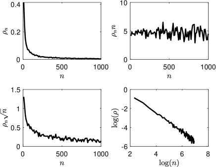
Figure 1: $\rho_{n}$ VS $n$ for 1-dimension normal distribution

	$\log(n)$	constant
Coefficient	-1.0037	1.5525
95% Confidence interval	[-1.0387,-0.9687]	[1.3419,1.7631]

Table 1: Regression results for 1-dimension normal distribution

We provide additional examples involving higher dimensions. In the subsequent examples, the data is sampled from a normal distribution $N(0,\Sigma_{0})$, where $\left(\Sigma_{0}\right)_{ij}=10\times 0.5^{|i-j|},$ $1\leq i,j\leq d$. We test the cases corresponding to $d=3$ and $d=5$ in the experiments. Due to computational constraints, we vary the number of data points, $n$, ranging from 20 to 400. For each $n$, we use $T=100$ trials to compute empirically the optimal choice of uncertainty to minimize the empirical Stein loss. Figures 2 and 3 show the results for the 3-dimension and 5-dimension cases, respectively. Tables 2 and 3 give the regression statistics and $R^{2}=0.97$ in both cases, and the performance is completely analogous to the one dimensional case, thus empirically validating our theoretical results.

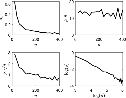
Figure 2: $\rho_{n}$ VS $n$ for 3-dimension normal distribution

	$\log(n)$	constant
Coefficient	-1.0340	2.7305
95% Confidence interval	[-1.1163,-0.9516]	[2.3045, 3.1565]

Table 2: Regression results for 3-dimension normal distribution

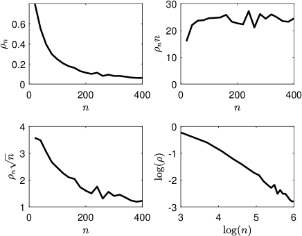
Figure 3: $\rho_{n}$ VS $n$ for 5-dimension normal distribution

	$\log(n)$	constant
Coefficient	-0.9177	2.7413
95% Confidence interval	[-0.9716 ,-0.8638]	[2.4625, 3.0201]

Table 3: Regression results for 5-dimension normal distribution

Appendix A Proofs of Auxiliary Results

Appendix A.1 Proof of Lemma 1

We first restate a theorem in [9].

Theorem 2 (Theorem 3.1 in [9]).

If $\rho>0$ and $\hat{\Sigma}_{n}$ admits the spectral decomposition $\hat{\Sigma}_{n}=\sum_{i=1}^{d}\hat{\lambda}_{i}\hat{v}_{i}\left(\hat{v}_{i}\right)^{T}$ with eigenvalues $\hat{\lambda}_{i}$ and corresponding orthonormal eigenvectors $\hat{v}_{i},$ $i\leq d,$ then the unique minimizer of (1) is given by $X_{n}^{\ast}(\rho)=\sum_{i=1}^{d}x_{i}^{\ast}\hat{v}_{i}\left(\hat{v}_{i}\right)^{T},$ where

$$\hat{x}_{i}^{\ast}=\gamma^{\ast}\left[1-\frac{1}{2}\left(\sqrt{\hat{\lambda}_{i}^{2}\left(\gamma^{\ast}\right)^{2}+4\hat{\lambda}_{i}\gamma^{\ast}}-\hat{\lambda}_{i}\gamma^{\ast}\right)\right],$$ (A.1)

and $\gamma^{\ast}>0$ is the unique positive solution of the algebraic equation

$$\left(\rho^{2}-\frac{1}{2}\sum_{i=1}^{d}\hat{\lambda}_{i}\right)\gamma-d+\frac{1}{2}\sum_{i=1}^{d}\sqrt{\hat{\lambda}_{i}^{2}\gamma^{2}+4\hat{\lambda}_{i}\gamma}=0.$$ (A.2)

Proof of Lemma 1..

Since the underlying covariance matrix is invertible with probability one when $n>d$, we have $\hat{\lambda}_{i}>0$ for $i=1,2,\ldots,d$. We consider the case $\rho\leq 1$. Note that we have the following inequality,

$$\sqrt{\hat{\lambda}_{i}^{2}\gamma^{2}+4\hat{\lambda}_{i}\gamma}-\left(\hat{\lambda}_{i}\gamma+2\right)=-\frac{4}{\sqrt{\hat{\lambda}_{i}^{2}\gamma^{2}+4\hat{\lambda}_{i}\gamma}+\left(\hat{\lambda}_{i}\gamma+2\right)}\geq-\frac{2}{\hat{\lambda}_{i}\gamma}.$$ (A.3)

Then, (A.2) gives us $\rho\gamma^{\ast}\leq\sqrt{\sum_{i=1}^{d}\hat{\lambda}_{i}^{-1}}.$ On the other hand, we have

$$\rho^{2}\gamma^{\ast} = \frac{1}{2}\sum_{i=1}^{d}\left(2+\hat{\lambda}_{i}\gamma^{\ast}-\sqrt{\hat{\lambda}_{i}^{2}\left(\gamma^{\ast}\right)^{2}+4\hat{\lambda}_{i}\gamma^{\ast}}\right)$$

$$= \sum_{i=1}^{d}\frac{2}{\sqrt{\hat{\lambda}_{i}^{2}\left(\gamma^{\ast}\right)^{2}+4\hat{\lambda}_{i}\left(\gamma^{\ast}\right)^{2}}+\left(\hat{\lambda}_{i}\gamma^{\ast}+2\right)}$$

$$\geq \sum_{i=1}^{d}\frac{1}{\hat{\lambda}_{i}\gamma^{\ast}+2}$$

$$\geq d\frac{1}{\left(\max_{i}\hat{\lambda}_{i}\right)\gamma^{\ast}+2}.$$

Then, a basic property of the quadratic equation gives us that

$$\gamma^{\ast}\geq\frac{\sqrt{1+\left(\max_{i}\hat{\lambda}_{i}\right)d/\rho^{2}}-1}{\left(\max_{i}\hat{\lambda}_{i}\right)}\geq\frac{1}{4}\min\left\{d/\rho^{2},\frac{\sqrt{d}/\rho}{\sqrt{\max_{i}\hat{\lambda}_{i}}}\right\}.$$

Furthermore, (Appendix A.1) also shows that

$$\rho^{2}\gamma^{\ast} \geq \left(\sum_{i=1}^{d}\frac{1}{\hat{\lambda}_{i}\gamma^{\ast}}\right)\frac{1}{1+2/\left(\left(\min_{i}\hat{\lambda}_{i}\right)\gamma^{\ast}\right)}$$ (A.5)

$$\geq \frac{1}{\gamma^{\ast}}\left(\sum_{i=1}^{d}\hat{\lambda}_{i}^{-1}\right)\frac{\min\left\{d/\rho^{2},\frac{\sqrt{d}/\rho}{\sqrt{\max_{i}\hat{\lambda}_{i}}}\right\}}{\min\left\{d/\rho^{2},\frac{\sqrt{d}/\rho}{\sqrt{\max_{i}\hat{\lambda}_{i}}}\right\}+8/\left(\min_{i}\hat{\lambda}_{i}\right)}.$$

By combining all of the above and noticing that $1+x\geq\sqrt{1+x}$ for $x\geq 0$, we have for $\rho\leq 1$

$$\frac{\rho}{\sqrt{\sum_{i=1}^{d}\hat{\lambda}_{i}^{-1}}}+\frac{\hat{M}_{n}}{\sqrt{\sum_{i=1}^{d}\hat{\lambda}_{i}^{-1}}}\rho^{2}\geq\frac{1}{\gamma^{\ast}}\geq\frac{1}{\sqrt{\sum_{i=1}^{d}\hat{\lambda}_{i}^{-1}}}\rho,$$ (A.6)

where

$$\hat{M}_{n}=\frac{8/\left(\min_{i}\hat{\lambda}_{i}\right)}{\min\left\{d,\frac{\sqrt{d}}{\sqrt{\max_{i}\hat{\lambda}_{i}}}\right\}}.$$

By plugging it to (A.2), we have

$$\frac{1}{x_{i}^{\ast}}=\frac{\sqrt{\hat{\lambda}_{i}^{2}\left(\gamma^{\ast}\right)^{2}+4\hat{\lambda}_{i}\gamma^{\ast}}+\hat{\lambda}_{i}\gamma^{\ast}+2}{2\gamma^{\ast}}\leq\hat{\lambda}_{i}+2/\gamma^{\ast}\leq\hat{\lambda}_{i}+\frac{2\rho}{\sqrt{\sum_{i=1}^{d}\hat{\lambda}_{i}^{-1}}}+\frac{2\hat{M}_{n}}{\sqrt{\sum_{i=1}^{d}\hat{\lambda}_{i}^{-1}}}\rho^{2}.$$

For the lower bound of $1/x_{i}^{\ast}$, we have

$$1/x_{i}^{\ast}=\frac{\sqrt{\hat{\lambda}_{i}^{2}\left(\gamma^{\ast}\right)^{2}+4\hat{\lambda}_{i}\gamma^{\ast}}+\hat{\lambda}_{i}\gamma^{\ast}+2}{2\gamma^{\ast}}\geq\frac{\sqrt{\hat{\lambda}_{i}^{2}\left(\gamma^{\ast}\right)^{2}+4\hat{\lambda}_{i}\gamma^{\ast}}}{\gamma^{\ast}}.$$

Then by (A.3), we have for $\rho\leq 1$

$$\frac{\sqrt{\hat{\lambda}_{i}^{2}\left(\gamma^{\ast}\right)^{2}+4\hat{\lambda}_{i}\gamma^{\ast}}}{\gamma^{\ast}} \geq \hat{\lambda}_{i}+2/\gamma^{\ast}-\frac{2}{\hat{\lambda}_{i}\left(\gamma^{\ast}\right)^{2}}$$

$$\geq \hat{\lambda}_{i}+\frac{2\rho}{\sqrt{\sum_{i=1}^{d}\hat{\lambda}_{i}^{-1}}}-\frac{2\left(1+\hat{M}_{n}\right)^{2}}{\hat{\lambda}_{i}\left(\sum_{i=1}^{d}\hat{\lambda}_{i}^{-1}\right)}\rho^{2}$$

Therefore, we conclude that

$$\frac{1}{x_{i}^{\ast}}=\hat{\lambda}_{i}+\frac{2\rho}{\sqrt{\sum_{i=1}^{d}\hat{\lambda}_{i}^{-1}}}+O(\rho^{2}).$$

and

$$X_{n}^{\ast}(\rho)^{-1}=\hat{\Sigma}_{n}-\hat{\Sigma}_{n}\hat{A}_{n}\hat{\Sigma}_{n}\rho+O(\rho^{2}),$$

where

$$\hat{A}_{n}=-\sum_{i=1}^{d}\frac{2\hat{v}_{i}\left(\hat{v}_{i}\right)^{T}}{\hat{\lambda}_{i}^{2}\sqrt{\sum_{i=1}^{d}\hat{\lambda}_{i}^{-1}}}=-\frac{2}{\sqrt{\text{tr}(\hat{\Sigma}_{n}^{-1})}}\hat{\Sigma}_{n}^{-2}.$$

Specifically, the remainder terms satisfy

$$-\left(\frac{2\left(1+\hat{M}_{n}\right)^{2}}{\sum_{i=1}^{d}\hat{\lambda}_{i}^{-1}}\sum_{i=1}^{d}\frac{\hat{v}_{i}\left(\hat{v}_{i}\right)^{T}}{\hat{\lambda}_{i}}\right)\rho^{2}\preceq X_{n}^{\ast}(\rho)^{-1}-\hat{\Sigma}_{n}+\hat{\Sigma}_{n}\hat{A}_{n}\hat{\Sigma}_{n}\rho\preceq\left(\frac{2\hat{M}_{n}}{\sqrt{\sum_{i=1}^{d}\hat{\lambda}_{i}^{-1}}}\sum_{i=1}^{d}\hat{v}_{i}\left(\hat{v}_{i}\right)^{T}\right)\rho^{2}.$$

We complete the proof of (4).

For the the proof of (3), note that (A.2) indicates

$$\frac{d\gamma^{\ast}}{d\rho} = \frac{-2\rho\gamma^{\ast}}{\left(\rho^{2}-\frac{1}{2}\sum_{i=1}^{d}\hat{\lambda}_{i}\right)+\frac{1}{2}\sum_{i=1}^{d}\hat{\lambda}_{i}\frac{\hat{\lambda}_{i}\gamma^{\ast}+2}{\sqrt{\hat{\lambda}_{i}^{2}\left(\gamma^{\ast}\right)^{2}+4\hat{\lambda}_{i}\gamma^{\ast}}}}$$

$$= -\frac{2\rho\gamma^{\ast}}{\rho^{2}+\sum_{i=1}^{d}\frac{2\hat{\lambda}_{i}}{\sqrt{\hat{\lambda}_{i}^{2}\left(\gamma^{\ast}\right)^{2}+4\hat{\lambda}_{i}\gamma^{\ast}}\left(\hat{\lambda}_{i}\gamma^{\ast}+2+\sqrt{\hat{\lambda}_{i}^{2}\left(\gamma^{\ast}\right)^{2}+4\hat{\lambda}_{i}\gamma^{\ast}}\right)}}.$$

Since $\hat{\lambda}_{i}\gamma^{\ast}\leq\sqrt{\hat{\lambda}_{i}^{2}\left(\gamma^{\ast}\right)^{2}+4\hat{\lambda}_{i}\gamma^{\ast}}\leq\hat{\lambda}_{i}\gamma^{\ast}+2$ and $\rho\gamma^{\ast}\leq\sqrt{\sum_{i=1}^{d}\hat{\lambda}_{i}^{-1}},$ we have

$$-\frac{2\rho\gamma^{\ast}}{\rho^{2}+\sum_{i=1}^{d}\frac{\hat{\lambda}_{i}}{\left(\hat{\lambda}_{i}\gamma^{\ast}+2\right)^{2}}}\leq\frac{\partial\gamma^{\ast}}{\partial\rho}\leq-\frac{2\rho\gamma^{\ast}}{\rho^{2}+\sum_{i=1}^{d}\frac{\hat{\lambda}_{i}}{\left(\hat{\lambda}_{i}\gamma^{\ast}\right)^{2}}}\leq-\frac{\rho\left(\gamma^{\ast}\right)^{3}}{\sum_{i=1}^{d}\hat{\lambda}_{i}^{-1}}.$$

Then, by using the bound (A.6), we further have

$$-\frac{\rho\left(\gamma^{\ast}\right)^{3}}{\sum_{i=1}^{d}\hat{\lambda}_{i}^{-1}}\leq-\frac{\left(\gamma^{\ast}\right)^{2}}{\sqrt{\sum_{i=1}^{d}\hat{\lambda}_{i}^{-1}}}\left(1-\hat{M}_{n}\rho\right).$$

Furthermore, the proof of Proposition 3.5 in [9] indicates that

$$\frac{\partial x_{i}}{\partial\gamma^{\ast}}=1+\hat{\lambda}_{i}\gamma^{\ast}-\frac{\hat{\lambda}_{i}^{2}\left(\gamma^{\ast}\right)^{2}+3\hat{\lambda}_{i}\gamma^{\ast}}{\sqrt{\hat{\lambda}_{i}^{2}\left(\gamma^{\ast}\right)^{2}+4\hat{\lambda}_{i}\gamma^{\ast}}}.$$

Let $z_{i}=\hat{\lambda}_{i}\gamma^{\ast}$ for $i=1,2,\ldots,d.$ We have

$$\frac{\partial x_{i}}{\partial\gamma^{\ast}}=\frac{4z_{i}}{\sqrt{z_{i}^{2}+4z_{i}}\left(\left(1+z_{i}\right)\sqrt{z_{i}^{2}+4z_{i}}+z_{i}^{2}+3z_{i}\right)}\in\left[\frac{2z_{i}}{\left(z_{i}+2\right)^{3}},\frac{2}{z_{i}^{2}}\right].$$

From (A.5), we have

$$\sum_{i=1}^{d}\frac{\hat{\lambda}_{i}}{\left(\hat{\lambda}_{i}\gamma^{\ast}+2\right)^{2}}\geq\frac{1}{\left(\gamma^{\ast}\right)^{2}}\left(\sum_{i=1}^{d}\hat{\lambda}_{i}^{-1}\right)\left(\frac{\min\left\{d/\rho^{2},\frac{\sqrt{d}/\rho}{\sqrt{\max_{i}\hat{\lambda}_{i}}}\right\}}{\min\left\{d/\rho^{2},\frac{\sqrt{d}/\rho}{\sqrt{\max_{i}\hat{\lambda}_{i}}}\right\}+8/\left(\min_{i}\hat{\lambda}_{i}\right)}\right)^{2}$$ (A.7)

and

$$\frac{2z_{i}}{\left(z_{i}+2\right)^{3}}\geq\frac{2}{\left(\hat{\lambda}_{i}\gamma^{\ast}\right)^{2}}\left(\frac{\min\left\{d/\rho^{2},\frac{\sqrt{d}/\rho}{\sqrt{\max_{i}\hat{\lambda}_{i}}}\right\}}{\min\left\{d/\rho^{2},\frac{\sqrt{d}/\rho}{\sqrt{\max_{i}\hat{\lambda}_{i}}}\right\}+8/\left(\min_{i}\hat{\lambda}_{i}\right)}\right)^{3}.$$

Therefore, by combining (A.5) and (A.7), we have for $\rho\leq 1,$

$$\frac{\partial\gamma^{\ast}}{\partial\rho} \geq -\frac{2\rho\left(\gamma^{\ast}\right)^{3}}{\left(\sum_{i=1}^{d}\hat{\lambda}_{i}^{-1}\right)\left(\frac{\min\left\{d/\rho^{2},\frac{\sqrt{d}/\rho}{\sqrt{\max_{i}\hat{\lambda}_{i}}}\right\}}{\min\left\{d/\rho^{2},\frac{\sqrt{d}/\rho}{\sqrt{\max_{i}\hat{\lambda}_{i}}}\right\}+8/\left(\min_{i}\hat{\lambda}_{i}\right)}+\left(\frac{\min\left\{d/\rho^{2},\frac{\sqrt{d}/\rho}{\sqrt{\max_{i}\hat{\lambda}_{i}}}\right\}}{\min\left\{d/\rho^{2},\frac{\sqrt{d}/\rho}{\sqrt{\max_{i}\hat{\lambda}_{i}}}\right\}+8/\left(\min_{i}\hat{\lambda}_{i}\right)}\right)^{2}\right)}$$

$$\geq -\frac{\rho\left(\gamma^{\ast}\right)^{3}}{\left(\sum_{i=1}^{d}\hat{\lambda}_{i}^{-1}\right)}\left(1+\hat{M}_{n}\rho\right)^{2}$$

$$\geq -\frac{\rho\left(\gamma^{\ast}\right)^{3}}{\left(\sum_{i=1}^{d}\hat{\lambda}_{i}^{-1}\right)}\left(1+\left(2\hat{M}_{n}+\hat{M}_{n}^{2}\right)\rho\right).$$

Similarly, we have for $\rho\leq 1,$

$$\frac{2z_{i}}{\left(z_{i}+2\right)^{3}}\geq\frac{2}{\left(\hat{\lambda}_{i}\gamma^{\ast}\right)^{2}}\left(1-\hat{M}_{n}\rho\right)^{3}\geq\frac{2}{\left(\hat{\lambda}_{i}\gamma^{\ast}\right)^{2}}\left(1-\left(\hat{M}_{n}^{3}+3\hat{M}_{n}\right)\rho\right).$$

Finally,  by combining all of the above together and the chain rule, we have

$$-\frac{2}{\hat{\lambda}_{i}^{2}}\frac{\rho\gamma^{\ast}}{\left(\sum_{i=1}^{d}\hat{\lambda}_{i}^{-1}\right)}\left(1+\left(2\hat{M}_{n}+\hat{M}_{n}^{2}\right)\rho\right)\leq\frac{\partial x_{i}}{\partial\rho}\leq-\frac{2}{\hat{\lambda}_{i}^{2}\sqrt{\sum_{i=1}^{d}\hat{\lambda}_{i}^{-1}}}\left(1-\hat{M}_{n}\rho\right)\left(1-\left(\hat{M}_{n}^{3}+3\hat{M}_{n}\right)\rho\right).$$

After simplification, we have

$$-\frac{\left(4\hat{M}_{n}+2\hat{M}_{n}^{2}\right)}{\hat{\lambda}_{i}^{2}\sqrt{\sum_{i=1}^{d}\hat{\lambda}_{i}^{-1}}}\rho\leq\frac{\partial x_{i}}{\partial\rho}+\frac{2}{\hat{\lambda}_{i}^{2}\sqrt{\sum_{i=1}^{d}\hat{\lambda}_{i}^{-1}}}\leq\frac{\left(2\hat{M}_{n}^{3}+8\hat{M}_{n}\right)}{\hat{\lambda}_{i}^{2}\sqrt{\sum_{i=1}^{d}\hat{\lambda}_{i}^{-1}}}\rho.$$

Furthermore, we have

$$-\left(\frac{4\hat{M}_{n}+2\hat{M}_{n}^{2}}{\sqrt{\sum_{i=1}^{d}\hat{\lambda}_{i}^{-1}}}\sum_{i=1}^{d}\frac{\hat{v}_{i}\left(\hat{v}_{i}\right)^{T}}{\hat{\lambda}_{i}^{2}}\right)\rho\preceq\frac{\partial X_{n}^{\ast}(\rho)}{\partial\rho}-\hat{A}_{n}\preceq\left(\frac{2\hat{M}_{n}^{3}+8\hat{M}_{n}}{\sqrt{\sum_{i=1}^{d}\hat{\lambda}_{i}^{-1}}}\sum_{i=1}^{d}\frac{\hat{v}_{i}\left(\hat{v}_{i}\right)^{T}}{\hat{\lambda}_{i}^{2}}\right)\rho.$$

This completes the proof. ∎

Appendix A.2 Proof of Proposition 1

Proof of (1)..

The proof follows from the standard central limit theorem (CLT). ∎

Proof of (2)..

Since $\hat{\Sigma}_{n}$ is the average of i.i.d copies $\xi_{i}\xi_{i}^{T},$ the result follows by CLT. ∎

Proof of (3)..

The first statement follows from the continuous mapping theorem and $\hat{\Sigma}_{n}\overset{p}{\rightarrow}\Sigma_{0}.$ Let $f(\Sigma)=-2\left(\text{tr}(\Sigma^{-1})\right)^{-1/2}\Sigma^{-2}$, where $\Sigma$ is positive-definite matrix. We now expand $f\left(\Sigma+hA\right)$ for any matrix $A$ as the scalar $h>0$ tends to zero to obtain a representation for the gradient of $f(\Sigma)$, $Df(\Sigma)$. This expansion yields

$$f\left(\Sigma+hA\right) = -2\left(\text{tr}(\left(\Sigma+hA\right)^{-1})\right)^{-1/2}\left(\Sigma+hA\right)^{-2}$$

$$= -2\left(\text{tr}(\Sigma^{-1})-\text{tr}\left(h\Sigma^{-1}A\Sigma^{-1}\right)+o\left(h\right)\right)^{-1/2}\left(\left(I+h\Sigma^{-1}A\right)^{-1}\Sigma^{-1}\right)^{2}$$

$$= -2\text{tr}(\Sigma^{-1})^{-1/2}\left(1-h\frac{\text{tr}\left(\Sigma^{-1}A\Sigma^{-1}\right)}{\text{tr}(\Sigma^{-1})}\right)^{-1/2}\left(\Sigma^{-2}-h\Sigma^{-1}A\Sigma^{-2}-h\Sigma^{-2}A\Sigma^{-1}\right)+o\left(h\right)$$

$$= -2\text{tr}(\Sigma^{-1})^{-1/2}\left(1+h\frac{\text{tr}\left(\Sigma^{-1}A\Sigma^{-1}\right)}{2\text{tr}(\Sigma^{-1})}\right)\left(\Sigma^{-2}-h\Sigma^{-1}A\Sigma^{-2}-h\Sigma^{-2}A\Sigma^{-1}\right)+o\left(h\right)$$

$$= -2\text{tr}(\Sigma^{-1})^{-1/2}\left(\Sigma^{-2}+h\frac{\text{tr}\left(\Sigma^{-1}A\Sigma^{-1}\right)\Sigma^{-2}}{2\text{tr}(\Sigma^{-1})}-h\Sigma^{-1}A\Sigma^{-2}-h\Sigma^{-2}A\Sigma^{-1}\right)+o\left(h\right)$$

$$= f\left(\Sigma\right)-h\frac{\text{tr}\left(\Sigma^{-1}A\Sigma^{-1}\right)\Sigma^{-2}}{\text{tr}(\Sigma^{-1})^{3/2}}+2h\frac{\Sigma^{-1}A\Sigma^{-2}+\Sigma^{-2}A\Sigma^{-1}}{\text{tr}(\Sigma^{-1})^{1/2}}+o\left(h\right),$$

which, in turn, results in the linear operator satisfying for any $A\in\mathbb{R}^{d\times d}$

$$Df(\Sigma)A=-\frac{\text{tr}\left(\Sigma^{-1}A\Sigma^{-1}\right)\Sigma^{-2}}{\text{tr}(\Sigma^{-1})^{3/2}}+2\frac{\Sigma^{-1}A\Sigma^{-2}+\Sigma^{-2}A\Sigma^{-1}}{\text{tr}(\Sigma^{-1})^{1/2}}.$$ (A.8)

After applying the delta method, we have the desired result. ∎

Appendix A.3 Proof of Proposition 2

We first note the following elementary result, which is standard in matrix algebra.

Lemma 3.

For any $d\times d$ matrices $A,B$ (real valued) we have

$$\text{tr}(A^{T}A)\text{tr}(B^{T}B)\geq\text{tr}(A^{T}B)^{2}=\left|\left\langle A,B\right\rangle\right|^{2},$$

where strict inequality holds unless $A$ is a multiple of $B$.

Proof of Lemma 3.

By the Cauchy-Schwarz inequality, we have

$$\text{tr}(A^{T}A)\text{tr}(B^{T}B)=\left(\sum_{i,j}A_{ij}^{2}\right)\left(\sum_{i,j}B_{ij}^{2}\right)\geq\left(\sum_{i,j}A_{ij}B_{ij}\right)^{2}=\left|\left\langle A,B\right\rangle\right|^{2}.$$

∎

Now we proceed with the proof of Proposition 2.

Proof of (1).

It suffices to show that $\left\langle Z,Z_{A}\right\rangle\geq 0$ with probability one and that $\left\langle Z,Z_{A}\right\rangle>0$ with positive probability. Note that

$$\left\langle Z,Z_{A}\right\rangle=-\frac{\text{tr}(Z\Sigma_{0}^{-2})^{2}}{\text{tr}(\Sigma_{0}^{-1})^{3/2}}+\frac{4\text{tr}\left(\Sigma_{0}^{-1}Z\Sigma_{0}^{-2}Z\right)}{\text{tr}(\Sigma_{0}^{-1})^{1/2}}.$$

We will show that

$$\text{tr}(\Sigma_{0}^{-1})\text{tr}\left(\Sigma_{0}^{-1}Z\Sigma_{0}^{-2}Z\right)\geq\text{tr}(Z\Sigma_{0}^{-2})^{2}$$ (A.9)

follows from Lemma 3. This implies that $\left\langle Z,Z_{A}\right\rangle\geq 0$. The equality holds if and only if there exists $a\geq 0$ such that $Z\Sigma_{0}^{-2}Z=aI,$ which is equivalent to $Z=\sqrt{a}\Sigma_{0}$. We know that $Z\neq\sqrt{a}\Sigma_{0}$ with probability one. Thus, $\left\langle Z,Z_{A}\right\rangle>0$ with probability one.

To show (A.9), we use the Polar factorization (see, for example, Chapter 4.2 in [6]) for positive definite matrices. That is, we write $\Sigma_{0}^{1/2}\Sigma_{0}^{1/2}=\Sigma_{0}$, where $\Sigma_{0}^{1/2}$ is a symmetric positive definite matrix. Note that we can write

$$Z=\Sigma_{0}^{1/2}W\Sigma_{0}^{1/2},$$

where $W=\Sigma_{0}^{-1/2}Z\Sigma_{0}^{-1/2}$ is a symmetric matrix. To recover the matrices $A$ and $B$, we let

$$A=\Sigma_{0}^{-1/2}\text{, }S=\Sigma_{0}\text{ and }B=WS^{-1/2}.$$

Note that

$$\text{tr}\left(\Sigma_{0}^{-1}Z\Sigma_{0}^{-2}Z\right)=\text{tr}\left(Z\Sigma_{0}^{-1}\cdot\Sigma_{0}^{-1}Z\Sigma_{0}^{-1}\right)$$

$$= \text{tr}\left(S^{1/2}WS^{1/2}S^{-1/2}S^{-1/2}\cdot S^{-1/2}S^{-1/2}\left(S^{1/2}WS^{1/2}\right)S^{-1/2}S^{-1/2}\right)$$

$$= \text{tr}\left(S^{1/2}WS^{-1/2}\cdot S^{-1/2}WS^{-1/2}\right)=\text{tr}\left(S^{-1/2}WWS^{-1/2}\right)=\text{tr}\left(B^{T}B\right).$$

Therefore, this verifies that the choice of $B$ is consistent with the use of Lemma 3. Clearly, $AA^{T}=\Sigma_{0}^{-1}$, thus making this choice also consistent with Lemma 3. Finally, we have that

$$\text{tr}(Z\Sigma_{0}^{-2}) = \text{tr}(S^{1/2}WS^{1/2}S^{-1/2}S^{-1/2}\Sigma_{0}^{-1})$$

$$= \text{tr}(S^{1/2}WS^{-1/2}S^{-1/2}S^{-1/2})$$

$$= \text{tr}(WS^{-1/2}S^{-1/2})=\text{tr}(S^{-1/2}S^{-1/2}W)=\text{tr}\left(A^{T}B\right).$$

The result then follows. ∎

Proof of (2):.

$$\left\langle\hat{\Sigma}_{n}-\Sigma_{0},\hat{A}_{n}-A_{0}\right\rangle = -2\left\langle\hat{\Sigma}_{n}-\Sigma_{0},\frac{1}{\sqrt{\text{tr}(\hat{\Sigma}_{n}^{-1})}}\hat{\Sigma}_{n}^{-2}-\frac{1}{\sqrt{\text{tr}(\Sigma_{0}^{-1})}}\Sigma_{0}^{-2}\right\rangle$$

$$= 2\left(-\sqrt{\text{tr}(\hat{\Sigma}_{n}^{-1})}-\sqrt{\text{tr}(\Sigma_{0})}+\frac{\text{tr}(\hat{\Sigma}_{n}^{-1}\Sigma_{0}\hat{\Sigma}_{n}^{-1})}{\sqrt{\text{tr}(\hat{\Sigma}_{n}^{-1})}}+\frac{\text{tr}(\Sigma_{0}^{-1}\hat{\Sigma}_{n}\Sigma_{0}^{-1})}{\sqrt{\text{tr}(\Sigma_{0}^{-1})}}\right).$$

By Lemma (3) and similar arguments with (1), we have

$$\text{tr}(\hat{\Sigma}_{n}^{-1}\Sigma_{0}\hat{\Sigma}_{n}^{-1})\geq\frac{\text{tr}(\hat{\Sigma}_{n}^{-1})^{2}}{\text{tr}(\Sigma_{0}^{-1})}\text{ and tr}(\Sigma_{0}^{-1}\hat{\Sigma}_{n}\Sigma_{0}^{-1})\geq\frac{\text{tr}(\Sigma_{0}^{-1})^{2}}{\text{tr}(\hat{\Sigma}_{n}^{-1})}.$$ (A.11)

By plugging (A.11) into (Appendix A.3), we have

$$\left\langle\hat{\Sigma}_{n}-\Sigma_{0},\hat{A}_{n}-A_{0}\right\rangle\geq 2\left(-\sqrt{\text{tr}(\hat{\Sigma}_{n}^{-1})}-\sqrt{\text{tr}(\Sigma_{0})}+\frac{\text{tr}(\hat{\Sigma}_{n}^{-1})^{3/2}}{\text{tr}(\Sigma_{0}^{-1})}+\frac{\text{tr}(\Sigma_{0}^{-1})^{3/2}}{\text{tr}(\hat{\Sigma}_{n}^{-1})}\right).$$

Consider the function $g:\mathbb{R}_{+}\times\mathbb{R}_{+}\rightarrow\mathbb{R}$,

$$g(a,b)=-a-b+\frac{b^{3}}{a^{2}}+\frac{a^{3}}{b^{2}}=\frac{(a^{3}-b^{3})(a^{2}-b^{2})}{a^{2}b^{2}}\geq 0,$$

and the equality holds if $a=b.$ Since $\sqrt{\text{tr}(\hat{\Sigma}_{n}^{-1})}=\sqrt{\text{tr}(\Sigma_{0})}$ with probability zero, the desired result follows. ∎

Appendix A.4 Proof of Lemma 2

We first collect a few results from linear algebra (see, for example, equation (2.3.3) and (2.3.7) in [6]).

Lemma 4.

For any $d\times d$ matrix $A$ (real valued) we define $\left\|A\right\|_{F}^{2}=\left\langle A,A\right\rangle=\mathrm{tr}\left(A^{T}A\right)$ (the Frobenius norm) and let $\left\|A\right\|_{2}^{2}=\left|\lambda_{\max}\left(A^{T}A\right)\right|$ (where $\lambda_{\max}\left(B\right)$ is the eigenvalue of largest modulus of the matrix $B$). Then, for any $A,B$ matrices of size $d\times d$ with real valued elements we have

$$\left\|AB\right\|_{F}\leq\left\|A\right\|_{F}\left\|B\right\|_{F},\text{ \ }\left\|B\right\|_{2}\leq\left\|B\right\|_{F}.$$

In addition, we have the following properties of the distribution of $\hat{\Sigma}_{n}$, which follows the Wishart law (see, for example, Theorem 13.3.2 in [1]).

Lemma 5.

Assume $n>d.$ Let us write $\xi_{i}=C\zeta_{i}$ where $C\in\mathbb{R}^{d\times d}$ and $CC^{T}=\Sigma_{0}$ and put

$$S_{n}=C\left(\sum_{i=1}^{n}\zeta_{i}\zeta_{i}^{T}\right)C^{T}.$$

Note that $\hat{\Sigma}_{n}=S_{n}/n$. Then, $S_{n}$ follows Wishart distribution with parameters $d,n$ and $\Sigma_{0}$ (denoted as $W_{d}\left(n,\Sigma_{0}\right)$). Equivalently, $W=C^{-1}S_{n}\left(C^{T}\right)^{-1}$ is distributed $W_{d}\left(n,I\right),$ where $I$ denotes the $d\times d$ identity matrix. Moreover, the eigenvalue distribution of $W$ satisfies

$$f_{w_{\left(1\right)},...,w_{\left(d\right)}}\left(w_{1},...,w_{d}\right)$$

$$= c_{d}\prod\limits_{i=1}^{d}\frac{\exp\left(-w_{i}/2\right)}{2^{n/2}\Gamma\left(\left(n-i+1\right)/2\right)}w_{i}^{\left(n-d-1\right)/2}\prod\limits_{j>i}\left(w_{j}-w_{i}\right)\mathbb{I}\left(0<w_{1}<...<w_{d}\right).$$

where $\Gamma(\cdot)$ is the gamma function, $c_{d}$ is a constant independent of $n$, and $\mathbb{I}(\cdot)$ is the indicator function.

We are now ready to provide the proof of Lemma 2. By Proposition (1), Slutsky’s theorem, and the continuous mapping theorem, we have

$$\left\langle\hat{\Sigma}_{n}\hat{A}_{n}\hat{\Sigma}_{n},\hat{A}_{n}\right\rangle\overset{p}{\rightarrow}\left\langle\Sigma_{0}A_{0}\Sigma_{0},A_{0}\right\rangle,$$

$$\left\langle\sqrt{n}\left(\hat{\Sigma}_{n}-\Sigma_{0}\right),\hat{A}_{n}\right\rangle\Rightarrow\left\langle Z,A_{0}\right\rangle,$$

$$\left\langle\sqrt{n}\left(\hat{\Sigma}_{n}-\Sigma_{0}\right),\sqrt{n}\left(\hat{A}_{n}-A_{0}\right)\right\rangle\Rightarrow\left\langle Z,Z_{A}\right\rangle.$$

Therefore, to verify Lemma 2, we need to show the uniform integrability of $\left\langle\hat{\Sigma}_{n}\hat{A}_{n}\hat{\Sigma}_{n},\hat{A}_{n}\right\rangle,$ $\left\langle\sqrt{n}\left(\hat{\Sigma}_{n}-\Sigma_{0}\right),\hat{A}_{n}\right\rangle$ and $\left\langle\sqrt{n}\left(\hat{\Sigma}_{n}-\Sigma_{0}\right),\sqrt{n}\left(\hat{A}_{n}-A_{0}\right)\right\rangle.$ In turn, it suffices to verify that for some $r>1$ and some $n_{0}<\infty$ we have

$$\sup_{n\geq n_{0}}\mathbb{E}\left[\left|\left\langle\hat{\Sigma}_{n}\hat{A}_{n}\hat{\Sigma}_{n},\hat{A}_{n}\right\rangle\right|^{r}\right]<\infty,$$

$$\sup_{n\geq n_{0}}\mathbb{E}\left[\left|\left\langle\sqrt{n}\left(\hat{\Sigma}_{n}-\Sigma_{0}\right),\hat{A}_{n}\right\rangle\right|^{r}\right]<\infty,$$

$$\sup_{n\geq n_{0}}\mathbb{E}\left[\left|\left\langle\sqrt{n}\left(\hat{\Sigma}_{n}-\Sigma_{0}\right),\sqrt{n}\left(\hat{A}_{n}-A_{0}\right)\right\rangle\right|^{r}\right]<\infty,$$

(see, for example, Chapter 5 in [5]).

Proof of (1). .

From Lemma 5 we have

$$f_{w_{\left(1\right)},...,w_{\left(d\right)}}\left(w_{1},...,w_{d}\right)$$

$$= c_{d}\prod\limits_{i=1}^{d}\frac{\exp\left(-w_{i}/2\right)}{2^{n/2}\Gamma\left(\left(n-i+1\right)/2\right)}w_{i}^{\left(n-d-1\right)/2}\prod\limits_{j>i}\left(w_{j}-w_{i}\right)\mathbb{I}\left(0<w_{1}<...<w_{d}\right)$$

$$= c_{d}\prod\limits_{i=1}^{d}\left(\frac{\exp\left(-w_{i}/2\right)}{2^{n/2}\Gamma\left(\left(n-i+1\right)/2\right)}w_{i}^{\left(n-d-1\right)/2}w_{i}^{d-i}\prod\limits_{j>i}\left(w_{j}/w_{i}-1\right)\mathbb{I}\left(0<w_{1}<...<w_{d}\right)\right)$$

$$= c_{d}\prod\limits_{i=1}^{d}\left(\frac{\exp\left(-w_{i}/2\right)}{2^{n/2}\Gamma\left(\left(n-i+1\right)/2\right)}w_{i}^{\left(n-i+1\right)/2-1}w_{i}^{{(d-i)/2}}\prod\limits_{j>i}\left(w_{j}/w_{i}-1\right)\mathbb{I}\left(0<w_{1}<...<w_{d}\right)\right)$$

$$= c_{d}^{\prime}\left(\prod\limits_{i=1}^{d}f_{\chi_{n-i+1}^{2}}\left(w_{i}\right)\right)\prod\limits_{i=1}^{d}\left(\frac{w_{i}}{n}\right)^{{(d-i)/2}}\prod\limits_{j>i}\left[n^{1/2}\left(w_{j}/w_{i}-1\right)\right]\mathbb{I}\left(0<w_{1}<...<w_{d}\right),$$

where $f_{\chi_{n-i+1}^{2}}\left(\cdot\right)$ denotes the density of a chi-squared distribution with $n-i+1$ degrees of freedom and $c_{d}^{\prime}$ is another constant also independent of $n$. The previous identity can be interpreted as follows. Let $W^{\left(n\right)}:=(W_{\left(1\right)}^{\left(n\right)},...,W_{\left(d\right)}^{\left(n\right)})$ be the eigenvalues of a $W_{d}\left(n,I\right)$ random matrix, and let $\Lambda\left(n\right):=\left(\Lambda_{1}\left(n\right),...,\Lambda_{d}\left(n\right)\right)$ be independent random variables such that $\Lambda_{i}\left(n\right)\sim\chi_{n-i+1}^{2}$. Then for any positive (and measurable) function $g:\mathbb{R}^{d}\rightarrow[0,\infty)$, we have

$$\mathbb{E}\left[g\left(W^{\left(n\right)}\right)\right]$$ (A.12)

$$= c_{d}^{\prime}\mathbb{E}\left[g\left(\Lambda\left(n\right)\right)\prod\limits_{i=1}^{d}\left(\frac{\Lambda_{i}\left(n\right)}{n}\right)^{{(d-i)/2}}\prod\limits_{j>i}\left|n^{1/2}\left(\Lambda_{j}\left(n\right)/\Lambda_{i}\left(n\right)-1\right)\right|\mathbb{I}\left(0<\Lambda_{1}\left(n\right)<...<\Lambda_{d}\left(n\right)\right)\right]$$

$$\leq c_{d}^{\prime}\mathbb{E}\left[g\left(\Lambda\left(n\right)\right)\prod\limits_{i=1}^{d}\left(\frac{\Lambda_{i}\left(n\right)}{n}\right)^{{(d-i)/2}}\prod\limits_{j>i}\left|n^{1/2}\left(\Lambda_{j}\left(n\right)/\Lambda_{i}\left(n\right)-1\right)\right|\right]$$

$$\leq c_{d}^{\prime}\sqrt{\mathbb{E}\left[g\left(\Lambda\left(n\right)\right)^{2}\right]}\sqrt{\mathbb{E}\left[\left(\prod\limits_{i=1}^{d}\left(\frac{\Lambda_{i}\left(n\right)}{n}\right)^{{(d-i)/2}}\prod\limits_{j>i}\left|n^{1/2}\left(\Lambda_{j}\left(n\right)/\Lambda_{i}\left(n\right)-1\right)\right|\right)^{2}\right]}$$

$$\leq c_{d}^{\prime}\sqrt{\mathbb{E}\left[g\left(\Lambda\left(n\right)\right)^{2}\right]}\mathbb{E}^{1/4}\left(\prod\limits_{i=1}^{d}\left(\frac{\Lambda_{i}\left(n\right)}{n}\right)^{2{(d-i)}}\right)\mathbb{E}^{1/4}\left(\prod\limits_{j>i}\left|n^{1/2}\left(\Lambda_{j}\left(n\right)/\Lambda_{i}\left(n\right)-1\right)\right|^{4}\right),$$

where the last two inequalities are obtained by the Cauchy-Schwarz inequality. We will show $\sup_{n\geq n_{0}}\mathbb{E}\left[\left|\left\langle\hat{\Sigma}_{n}\hat{A}_{n}\hat{\Sigma}_{n},\hat{A}_{n}\right\rangle\right|^{r}\right]<\infty$ to verify the first statement of Lemma 2. Note that we can simplify $\left|\left\langle\hat{\Sigma}_{n}\hat{A}_{n}\hat{\Sigma}_{n},\hat{A}_{n}\right\rangle\right|^{r}$ as

$$\left|\left\langle\hat{\Sigma}_{n}\hat{A}_{n}\hat{\Sigma}_{n},\hat{A}_{n}\right\rangle\right|^{r}=\left|\text{tr}\left(\hat{A}_{n}\hat{\Sigma}_{n}\hat{A}_{n}\hat{\Sigma}_{n}\right)\right|^{r}=\frac{4^{r}}{\text{tr}\left(\hat{\Sigma}_{n}^{-1}\right)^{r}}\mathrm{tr}\left(\hat{\Sigma}_{n}^{-2}\right)^{r}.$$

By our definition, we have

$$\hat{\Sigma}_{n}^{-1}=\left(C^{T}\right)^{-1}\left(W/n\right)^{-1}C^{-1},$$

and thus there exist numerical constants $c$${}_{1},\bar{c}_{1}>0$ such that

$$\underline{c}_{1}\text{tr}\left(\left(W/n\right)^{-1}\right)\leq\text{tr}\left(\hat{\Sigma}_{n}^{-1}\right)\leq\bar{c}_{1}\text{tr}\left(\left(W/n\right)^{-1}\right).$$

Similarly, there exist numerical constants $c$${}_{2},\bar{c}_{2}>0$ such that

$$\underline{c}_{2}\text{tr}\left(\left(W/n\right)^{-2}\right)\leq\text{tr}\left(\hat{\Sigma}_{n}^{-2}\right)\leq\bar{c}_{2}\text{tr}\left(\left(W/n\right)^{-2}\right).$$

After using the Cauchy-Schwarz inequality again, we have

$$\mathbb{E}\left|\left\langle\hat{\Sigma}_{n}\hat{A}_{n}\hat{\Sigma}_{n},\hat{A}_{n}\right\rangle\right|^{r} \leq c\mathbb{E}\left[\sum_{i=1}^{d}\left(\frac{W_{\left(i\right)}^{\left(n\right)}}{n}\right)^{r}\sum_{i=1}^{d}\left(\frac{n}{W_{\left(i\right)}^{\left(n\right)}}\right)^{2r}\right]$$ (A.13)

$$\leq c\sqrt{\mathbb{E}\left[\sum_{i=1}^{d}\left(\frac{W_{\left(i\right)}^{\left(n\right)}}{n}\right)^{2r}\right]}\sqrt{\mathbb{E}\left[\sum_{i=1}^{d}\left(\frac{n}{W_{\left(i\right)}^{\left(n\right)}}\right)^{4r}\right]},$$

where $c$ is a numerical constant. Therefore, it suffices to show that for any $r>1$ there exists $n_{0}$ such that

$$\sup_{n\geq n_{0}}\left(\mathbb{E}\left[\left(\frac{\Lambda_{j}\left(n\right)}{n}\right)^{r}\right]\cdot\mathbb{E}\left[\left(\frac{n}{\Lambda_{i}\left(n\right)}\right)^{r}\right]\cdot\mathbb{E}\left[\left|n^{1/2}\left(\Lambda_{j}\left(n\right)/\Lambda_{i}\left(n\right)-1\right)\right|^{r}\right]\right)<\infty.$$ (A.14)

We know that $\Lambda_{i}\left(n\right)/n$ follows the gamma distribution with shape parameter $\alpha=\left(n-i+1\right)/2$ and scale parameter $\lambda=n/2$. Write $Y_{n}\sim Gamma\left(\alpha,\lambda\right)$ and note that

$$\mathbb{E}\left(\frac{1}{Y_{n}^{r}}\right) = \int_{0}^{\infty}\frac{1}{y^{r}}\frac{\exp\left(-\lambda y\right)\lambda^{\alpha}y^{\alpha-1}}{\Gamma\left(\alpha\right)}\mathrm{d}y$$ (A.15)

$$= \int_{0}^{\infty}\frac{\Gamma\left(\alpha-t\right)\lambda^{r}\exp\left(-\lambda y\right)\lambda^{\alpha-r}y^{\alpha-r-1}}{\Gamma\left(\alpha\right)\Gamma\left(\alpha-r\right)}\mathrm{d}y$$

$$= \frac{\Gamma\left(\alpha-r\right)\lambda^{r}}{\Gamma\left(\alpha\right)}.$$

It follows from standard properties of the gamma function that lim${}_{n\rightarrow\infty}\Gamma\left(\alpha-r\right)\lambda^{r}/\Gamma\left(\alpha\right)=1$ (see, for example, Chapter 3 in [7]). After applying exactly the same approach to $\mathbb{E}\left[\left(\Lambda_{i}\left(n\right)/n\right)^{r}\right]$, we have

$$\mathbb{E}\left[\left(\Lambda_{i}\left(n\right)/n\right)^{r}\right]=\frac{\Gamma\left(\alpha+r\right)}{\Gamma\left(\alpha\right)\lambda^{r}}\rightarrow 1,$$ (A.16)

as $n\rightarrow\infty.$

Now, we only need to show the third term in (A.14) is finite. Note that

$$\mathbb{E}\left[\left|n^{1/2}\left(\Lambda_{j}\left(n\right)/\Lambda_{i}\left(n\right)-1\right)\right|^{r}\right]$$

$$= \mathbb{E}\left[\left|n^{1/2}\left(\Lambda_{j}\left(n\right)/\Lambda_{i}\left(n\right)-1\right)\right|^{r}\mathbb{I}\left(\left|\Lambda_{j}\left(n\right)/n-1\right|\leq\varepsilon,\left|\Lambda_{i}\left(n\right)/n-1\right|\leq\varepsilon\right)\right]$$

$$+\mathbb{E}\left[\left|n^{1/2}\left(\Lambda_{j}\left(n\right)/\Lambda_{i}\left(n\right)-1\right)\right|^{r}\mathbb{I}\left(\left|\Lambda_{j}\left(n\right)/n-1\right|>\varepsilon\cup\left|\Lambda_{i}\left(n\right)/n-1\right|>\varepsilon\right)\right].$$

It is straightforward to verify (for example by computing moment generating functions of the Gamma distribution) that

$$\sup_{n\geq 1}\mathbb{E}\left(n^{r/2}\left|\frac{\Lambda_{j}\left(n\right)}{n}-1\right|^{r}\right)<\infty$$ (A.18)

for any $r>0$ and further, we can conclude that

$$\sup_{n\geq 1}\mathbb{E}\left[\left|n^{1/2}\left(\Lambda_{j}\left(n\right)/\Lambda_{i}\left(n\right)-1\right)\right|^{r}\mathbb{I}\left(\left|\Lambda_{j}\left(n\right)/n-1\right|\leq\varepsilon,\left|\Lambda_{i}\left(n\right)/n-1\right|\leq\varepsilon\right)\right]$$

$$\leq \sup_{n\geq 1}\mathbb{E}\left[\left|n^{1/2}\left(\left(\left(\frac{\Lambda_{j}\left(n\right)}{n}-1\right)-\left(\frac{\Lambda_{i}\left(n\right)}{n}-1\right)\right)/\left(1-\epsilon\right)\right)\right|^{r}\mathbb{I}\left(\left|\Lambda_{j}\left(n\right)/n-1\right|\leq\varepsilon,\left|\Lambda_{i}\left(n\right)/n-1\right|\leq\varepsilon\right)\right]$$

$$\leq \frac{2^{r-1}}{\left(1-\varepsilon\right)^{r}}\sup_{n\geq 1}\mathbb{E}\left(n^{r/2}\left|\frac{\Lambda_{j}\left(n\right)}{n}-1\right|^{r}\right)<\infty.$$

Then, because $\Lambda_{j}\left(n\right)/n$ (being the sum of $n-j+1$ i.i.d. random variables with finite moment generating function) satisfies the large deviations principle (see, for instance, Chapter 2.2 in [4]), we have

$$\mathbb{E}\left[\left|n^{1/2}\left(\Lambda_{j}\left(n\right)/\Lambda_{i}\left(n\right)-1\right)\right|^{r}\mathbb{I}\left(\left|\Lambda_{j}\left(n\right)/n-1\right|>\varepsilon\right)\right]$$ (A.19)

$$\leq \sqrt{\mathbb{E}\left[\left|n^{1/2}\left(\Lambda_{j}\left(n\right)/\Lambda_{i}\left(n\right)-1\right)\right|^{2r}\right]}\sqrt{\mathbb{P}\left(\left|\Lambda_{j}\left(n\right)/n-1\right|>\varepsilon\right)}.$$

Because of our discussion involving the finiteness of the first two factors in (A.14), we can conclude that when $n>d+8r$,

$$\sqrt{\mathbb{E}\left[\left|n^{1/2}\left(\Lambda_{j}\left(n\right)/\Lambda_{i}\left(n\right)-1\right)\right|^{2r}\right]} \leq n^{r}\sqrt{1+\mathbb{E}\left[\left(\frac{\Lambda_{j}\left(n\right)}{n}\times\frac{n}{\Lambda_{i}\left(n\right)}\right)^{2r}\right]}$$

$$\leq n^{r}\sqrt{1+\sqrt{\mathbb{E}\left(\left(\Lambda_{j}\left(n\right)/n\right)^{4r}\right)}\times\sqrt{\mathbb{E}\left(\left(n/\Lambda_{i}\left(n\right)\right)^{4r}\right)}}$$

$$\leq C_{r}^{\prime}n^{r}.$$

Notice that from A.15 and A.16, we have

$$\sup_{n>d+8r}\mathbb{E}\left(\left(\Lambda_{j}\left(n\right)/n\right)^{4r}\right)\times\mathbb{E}\left(\left(n/\Lambda_{i}\left(n\right)\right)^{4r}\right)<\infty,$$

which means $C_{r}^{\prime}$ is a numerical constant independent with $n$. Therefore, the first term in the right hand side of (A.19) grows at rate $O\left(n^{r}\right)$, which is polynomial, whereas the second term, due to the large deviations principle invoked earlier converges exponentially fast to zero for each $\varepsilon>0$. This completes the first part of Lemma 2. ∎

Proof of (2)..

For the second part of Lemma 2, note that Lemma 3 implies

$$\left|\left\langle\sqrt{n}\left(\hat{\Sigma}_{n}-\Sigma_{0}\right),\hat{A}_{n}\right\rangle\right|^{2}\leq\left\|\sqrt{n}\left(\hat{\Sigma}_{n}-\Sigma_{0}\right)\right\|_{F}^{2}\left\|\hat{A}_{n}\right\|_{F}^{2}.$$

Then, for the uniform integrability of $\left\|\sqrt{n}\left(\hat{\Sigma}_{n}-\Sigma_{0}\right)\right\|_{F}^{2},$ we have

$$\left\|\sqrt{n}\left(\hat{\Sigma}_{n}-\Sigma_{0}\right)\right\|_{F}^{4}=\left\|C\sqrt{n}\left(\frac{1}{n}\sum_{i=1}^{n}\zeta_{i}^{T}\zeta_{i}-I\right)C^{T}\right\|_{F}^{4}\leq\left\|\sqrt{n}\left(\frac{1}{n}\sum_{i=1}^{n}\zeta_{i}^{T}\zeta_{i}-I\right)\right\|_{F}^{4}\left\|C\right\|_{F}^{8},$$

by Lemma 4. We denote $\hat{\Psi}^{(n)}=\frac{1}{n}\sum_{i=1}^{n}\zeta_{i}^{T}\zeta_{i}.$ And by the Cauchy-Schwarz inequality, we have

$$\left\|\sqrt{n}\left(\frac{1}{n}\sum_{i=1}^{n}\zeta_{i}^{T}\zeta_{i}-I\right)\right\|_{F}^{4}=\left(\sum_{i,j}\left(\sqrt{n}\left(\hat{\Psi}_{ij}^{(n)}-\delta_{ij}\right)\right)^{2}\right)^{2}\leq d^{2}\sum_{i,j}\left(\sqrt{n}\left(\hat{\Psi}_{ij}^{(n)}-\delta_{ij}\right)\right)^{4},$$

where $\delta_{ij}=\mathbb{I}\{i=j\}.$ Note that

$$\mathbb{E}\left[\sum_{i,j}\left(\sqrt{n}\left(\hat{\Psi}_{ij}^{(n)}-\delta_{ij}\right)\right)^{4}\right]$$

$$= \mathbb{E}\left[\sum_{i=1}^{d}\left(\sqrt{n}\left(\left(\frac{1}{n}\sum_{k=1}^{n}z_{ik}^{2}\right)-1\right)\right)^{4}\right]+2\mathbb{E}\left[\sum_{i=1}^{d}\sum_{j=1+1}^{d}\left(\sqrt{n}\left(\frac{1}{n}\sum_{k=1}^{n}z_{ik}z_{jk}\right)\right)^{4}\right]$$

$$= d\mathbb{E}\left[\left(\frac{1}{\sqrt{n}}\sum_{k=1}^{n}\left(z_{ik}^{2}-1\right)\right)^{4}\right]+d(d-1)\mathbb{E}\left[\left(\frac{1}{\sqrt{n}}\sum_{k=1}^{n}z_{ik}z_{jk}\right)^{4}\right],$$

where $z_{ik}\sim N(0,1)$ are i.i.d random variables. Further, direct calculations give us

$$\mathbb{E}\left[\left(\frac{1}{\sqrt{n}}\sum_{k=1}^{n}\left(z_{ik}^{2}-1\right)\right)^{4}\right] = \frac{1}{n^{2}}\left(\mathbb{E}\left[\sum_{k=1}^{n}\left(z_{ik}^{2}-1\right)^{4}\right]+6\frac{1}{n^{2}}\mathbb{E}\left[\sum_{k=1}^{n}\sum_{l=k+1}^{n}\left(z_{ik}^{2}-1\right)^{2}\left(z_{il}^{2}-1\right)^{2}\right]\right)$$

$$= \frac{60}{n}+\frac{12(n-1)}{n}<\infty,$$

and

$$\mathbb{E}\left[\left(\frac{1}{\sqrt{n}}\sum_{k=1}^{n}z_{ik}z_{jk}\right)^{4}\right]=\frac{1}{n^{2}}\mathbb{E}\left[\sum_{k=1}^{n}z_{ik}^{4}z_{jk}^{4}\right]+6\frac{1}{n^{2}}\mathbb{E}\left[\sum_{k=1}^{n}\sum_{l=k+1}^{n}z_{ik}^{2}z_{jk}^{2}z_{il}^{2}z_{jl}^{2}\right]=\frac{9}{n}+\frac{3\left(n-1\right)}{n}<\infty.$$

Therefore, we complete the uniform integrability of $\left\|\sqrt{n}\left(\hat{\Sigma}_{n}-\Sigma_{0}\right)\right\|_{F}^{2}.$

For $\left\|\hat{A}_{n}\right\|_{F}^{2},$ using the similar argument with (A.13), we have

$$\left\|\hat{A}_{n}\right\|_{F}^{2r}=\left|\text{tr}(\hat{A}_{n}^{2})\right|^{r}=\frac{4^{r}\mathrm{tr}\left(\hat{\Sigma}_{n}^{-4}\right)^{r}}{\text{tr}\left(\hat{\Sigma}_{n}^{-1}\right)^{r}}\leq c_{2}\sqrt{\mathbb{E}\left[\sum_{i=1}^{d}\left(\frac{W_{\left(i\right)}^{\left(n\right)}}{n}\right)^{2r}\right]}\sqrt{\mathbb{E}\left[\sum_{i=1}^{d}\left(\frac{n}{W_{\left(i\right)}^{\left(n\right)}}\right)^{8r}\right]}.$$ (A.20)

From the earlier bounds leading to the analysis of (A.14), we complete the uniform integrability of $\left\|\hat{A}_{n}\right\|_{F}^{2}$. Hence, the second part of Lemma 2 follows. ∎

Proof of (3)..

For the third part of Lemma 2, recall in the proof of Proposition 1(3), $f(\Sigma)=-\frac{2}{\sqrt{\text{tr}(\Sigma^{-1})}}\Sigma^{-2}$ and thus $\hat{A}_{n}=f\left(\hat{\Sigma}_{n}\right)$.

The argument is similar to that given to establish (Appendix A.4). We have argued that $f\left(\cdot\right)$ is smooth around $\Sigma_{0}$, which was the basis for the use of the delta method earlier in our argument. Moreover, note that $\hat{\Sigma}_{n}$ satisfies a large deviations principle. Therefore

$$\left|\left\langle\sqrt{n}\left(\hat{\Sigma}_{n}-\Sigma_{0}\right),\sqrt{n}\left(\hat{A}_{n}-A_{0}\right)\right\rangle\right|$$

$$= \left|\left\langle\sqrt{n}\left(\hat{\Sigma}_{n}-\Sigma_{0}\right),\sqrt{n}\left(f\left(\hat{\Sigma}_{n}\right)-A_{0}\right)\right\rangle\right|$$

$$= \left|\left\langle\sqrt{n}\left(\hat{\Sigma}_{n}-\Sigma_{0}\right),\sqrt{n}\left(f\left(\hat{\Sigma}_{n}\right)-A_{0}\right)\right\rangle\right|\mathbb{I}\left(\left\|\hat{\Sigma}_{n}-\Sigma_{0}\right\|_{F}\leq\varepsilon\right)$$

$$+\left|\left\langle\sqrt{n}\left(\hat{\Sigma}_{n}-\Sigma_{0}\right),\sqrt{n}\left(f\left(\hat{\Sigma}_{n}\right)-A_{0}\right)\right\rangle\right|\mathbb{I}\left(\left\|\hat{\Sigma}_{n}-\Sigma_{0}\right\|_{F}>\varepsilon\right).$$

By applying Lemma 3 and the fact that $Df\left(\cdot\right)$ is continuous around $\Sigma_{0}$ (see the expression of $Df\left(\cdot\right)$ in (A.8)) we conclude that

$$\left|\left\langle\sqrt{n}\left(\hat{\Sigma}_{n}-\Sigma_{0}\right),\sqrt{n}\left(f\left(\hat{\Sigma}_{n}\right)-A_{0}\right)\right\rangle\right|\mathbb{I}\left(\left\|\hat{\Sigma}_{n}-\Sigma_{0}\right\|_{F}\leq\varepsilon\right)$$

$$\leq \sup_{\Sigma:\left\|\Sigma_{0}-\Sigma\right\|_{F}\leq\varepsilon}\left|\left\langle\sqrt{n}\left(\hat{\Sigma}_{n}-\Sigma_{0}\right),Df\left(\Sigma\right)\left(\sqrt{n}\left(\hat{\Sigma}_{n}-\Sigma_{0}\right)\right)\right\rangle\right|$$

$$\leq c_{0}\left\|\sqrt{n}\left(\hat{\Sigma}_{n}-\Sigma_{0}\right)\right\|_{F}^{2},$$

where $c_{0}=\sup_{\Sigma:\left\|\Sigma_{0}-\Sigma\right\|_{F}\leq\varepsilon}\left\|Df\left(\Sigma\right)\right\|_{op}$ and $\left\|Df\left(\Sigma\right)\right\|_{op}$ is the operator norm, which is defined by

$$\left\|Df\left(\Sigma\right)\right\|_{op}:=\sup\left\{\left\|Df\left(\Sigma\right)A\right\|_{F}:A\in\mathbb{R}^{d\times d}\text{ with }\|A\|_{F}=1\right\}.$$

Since $Df\left(\cdot\right)$ is continuous around $\Sigma_{0}$, there exists sufficient small $\epsilon$ such that $c_{0}$ is finite. $\left\|\sqrt{n}\left(\hat{\Sigma}_{n}-\Sigma_{0}\right)\right\|_{F}^{2}$ is proved to be uniformly integrable in the second part of Lemma 2. On the other hand, we have for $r>1$

$$\mathbb{E}\left[\left|\left\langle\sqrt{n}\left(\hat{\Sigma}_{n}-\Sigma_{0}\right),\sqrt{n}\left(f\left(\hat{\Sigma}_{n}\right)-A_{0}\right)\right\rangle\right|^{r}\mathbb{I}\left(\left\|\hat{\Sigma}_{n}-\Sigma_{0}\right\|_{F}>\varepsilon\right)\right]$$

$$\leq \mathbb{E}\left[\left\|\sqrt{n}\left(\hat{\Sigma}_{n}-\Sigma_{0}\right)\right\|_{F}^{r}\left\|\sqrt{n}\left(f\left(\hat{\Sigma}_{n}\right)-A_{0}\right)\right\|_{F}^{r}\mathbb{I}\left(\left\|\hat{\Sigma}_{n}-\Sigma_{0}\right\|_{F}>\varepsilon\right)\right]$$

$$\leq \sqrt{\mathbb{E}\left(\left\|\sqrt{n}\left(\hat{\Sigma}_{n}-\Sigma_{0}\right)\right\|_{F}^{2r}\right)}\mathbb{E}^{1/4}\left(\left\|\sqrt{n}\left(f\left(\hat{\Sigma}_{n}\right)-A_{0}\right)\right\|_{F}^{4r}\right)\left(\mathbb{P}\left(\left\|\hat{\Sigma}_{n}-\Sigma_{0}\right\|_{F}>\varepsilon\right)\right)^{1/4}.$$

The proof of the second part of Lemma 2 shows $\mathbb{E}\left(\left\|\sqrt{n}\left(\hat{\Sigma}_{n}-\Sigma_{0}\right)\right\|_{F}^{2r}\right)<\infty$ when $r\leq 2.$ Further, we have argued throughout the proof of the first part of Lemma 2 and the proof leading to (A.20) that

$$\mathbb{E}\left(\left\|\sqrt{n}\left(f\left(\hat{\Sigma}_{n}\right)-A_{0}\right)\right\|_{F}^{4r}\right)\leq c_{3}n^{2r}\left(\mathbb{E}\left(\left\|\hat{A}_{n}\right\|^{4r}\right)+\left\|A_{0}\right\|^{4r}\right)\leq O\left(n^{2r}\right),$$

where $c_{3}$ is a numerical constant only related to $r$ and $d$. However, the large deviations principle gives us $\mathbb{P}\left(\left\|\hat{\Sigma}_{n}-\Sigma_{0}\right\|_{F}>\varepsilon\right)=O\left(\exp\left(-cn\right)\right)$ for some $c>0$. Therefore, using Lemmas 3 and 4 and the previous estimates we can complete the last part of Lemma 2. ∎

Appendix A.5 Proof of Proposition 3

Proof.

Let $X^{\ast}(\rho):=\arg\min_{X\succ 0}\left\{-\log\det X+\sup_{\mathbb{Q}\in\mathcal{P}_{\rho}^{\ast}}\mathbb{E}^{\mathbb{Q}}\left[\left\langle\xi\xi^{T},X\right\rangle\right]\right\},$ where

$$\mathcal{P}_{\rho}^{\ast}=\left\{\mathbb{Q}\sim\mathcal{N}\left(0,\Sigma\right)\text{ for some }\Sigma:\mathbb{W}_{2}(\mathcal{N}\left(0,\Sigma_{0}\right),\mathbb{Q})\leq\rho\right\}.$$

Then, $\arg\min_{\rho\geq 0}\{\mathbb{E}[L(X^{\ast}(\rho),\Sigma_{0})]\}=0.$ Since $X_{n}^{\ast}(\rho)$ is a continuous function of $\hat{\Sigma}_{n},$ we have $X_{n}^{\ast}(\rho)\rightarrow$ $X^{\ast}(\rho)$ almost surely for all $\rho\geq 0$ by the continuous mapping theorem. Furthermore, proof of Lemma 2 gives us $\mathbb{E}X_{n}^{\ast}(0)=\mathbb{E}\hat{\Sigma}_{n}^{-1}\rightarrow\Sigma_{0}^{-1}.$ And from Lemmas 1 and 2 in [3], we have

$$\left|\log\det(\hat{\Sigma}_{n}^{-1})-\log\det(\Sigma_{0}^{-1})\right|=\left|\sum_{k=1}^{d}\log\left(\frac{1}{n}\chi_{n-k-1}^{2}\right)\right|\rightarrow 0,$$

where $\chi_{n}^{2},\ldots,\chi_{n-p-1}^{2}$ are mutually independent $\chi^{2}$ distribution with the degree of freedom $n,\ldots,n-p+1$ respectively. Due to the uniform integrability of $\log\left(\frac{1}{n}\chi_{n-k-1}^{2}\right)$, we conclude $\mathbb{E}\left[\log\det\left(X_{n}^{\ast}(0)\right)\right]\rightarrow\mathbb{E}\left[\log\det\left(X^{\ast}(0)\right)\right].$

By (A.2), (Appendix A.1) and (A.1), we have $x_{i}^{\ast}\leq\gamma^{\ast}\leq d/\rho^{2}$ and

$$\hat{x}_{i}^{\ast} = \gamma^{\ast}\left[1-\frac{1}{2}\left(\sqrt{\hat{\lambda}_{i}^{2}\left(\gamma^{\ast}\right)^{2}+4\hat{\lambda}_{i}\gamma^{\ast}}-\hat{\lambda}_{i}\gamma^{\ast}\right)\right]$$

$$\geq \frac{1}{\rho^{2}}\left(\sum_{i=1}^{d}\frac{1}{\hat{\lambda}_{i}\gamma^{\ast}+2}\right)\frac{1}{\hat{\lambda}_{i}\gamma^{\ast}+2}$$

$$\geq \frac{1}{\rho^{2}}\left(\frac{1}{\hat{\lambda}_{i}\gamma^{\ast}+2}\right)^{2}.$$

Therefore, we have

$$L(X_{n}^{\ast}(\rho),\Sigma_{0}) = -\log\det(X_{n}^{\ast}(\rho)\Sigma_{0})+\left\langle X_{n}^{\ast}(\rho),\Sigma_{0}\right\rangle-d$$

$$= -\log\det(X_{n}^{\ast}(\rho))+\left\langle X_{n}^{\ast}(\rho),\Sigma_{0}\right\rangle-\log\det(\Sigma_{0})-d$$

$$\geq d\log\left(\rho^{2}/d\right)-\log\det(\Sigma_{0})-d.$$

Thus, $\rho_{n}\in[0,C]$, for large enough $n$ and a large enough constant $C.$ By proposition 3.5 in [9], we have $\log\det(X_{n}^{\ast}(\rho))$ and $\left\langle X_{n}^{\ast}(\rho),\Sigma_{0}\right\rangle$ decrease with $\rho.$ Then, $\mathbb{E}\left\langle X_{n}^{\ast}(\rho),\Sigma_{0}\right\rangle\rightarrow\mathbb{E}\left\langle X^{\ast}(\rho),\Sigma_{0}\right\rangle$ since $\mathbf{0}\preceq X_{n}^{\ast}(\rho)\preceq X_{n}^{\ast}(0)=\hat{\Sigma}_{n}^{-1}$ and $\hat{\Sigma}_{n}^{-1}$ is uniformly integrable. For $\log\det(X_{n}^{\ast}(\rho)),$ the upper bound is given by

$$\log\det(X_{n}^{\ast}(\rho))\leq\log\det(\hat{\Sigma}_{n}^{-1}),$$

and the lower bound is given by

$$\log\det(X_{n}^{\ast}(\rho)) = \log\left(\prod\limits_{i=1}^{d}\hat{x}_{i}^{\ast}\right)$$

$$\geq \log\left(\prod\limits_{i=1}^{d}\frac{1}{\rho^{2}}\left(\frac{1}{\hat{\lambda}_{i}\gamma^{\ast}+2}\right)^{2}\right)$$

$$\geq -2d\log\rho-2\sum_{i=1}^{d}\left(\log\left(\hat{\lambda}_{i}\left(d/\rho^{2}\right)+2\right)\right)$$

$$\geq -2d\log\rho-2\log\det\left(\left(d/\rho^{2}\right)\hat{\Sigma}_{n}+2I\right).$$

Due to the uniform integrability of $\log\det\left(\left(d/\rho^{2}\right)\hat{\Sigma}_{n}+2I\right)$ and $\log\det(\hat{\Sigma}_{n}^{-1}),$ we have $\mathbb{E}\left[\log\det(X_{n}^{\ast}(\rho))\right]\rightarrow\mathbb{E}\left[\log\det(X^{\ast}(\rho))\right].$ Finally, by the monotonicity of $\mathbb{E}\left[\log\det(X_{n}^{\ast}(\rho))\right]$ and $\mathbb{E}\left\langle X_{n}^{\ast}(\rho),\Sigma_{0}\right\rangle,$ we have $\mathbb{E}\left[L(X_{n}^{\ast}(\rho),\Sigma_{0})\right]$ converges uniformly; thus, $\rho_{n}\rightarrow\arg\min_{\rho\geq 0}\{\mathbb{E}[L(X^{\ast}(\rho),\Sigma_{0})]\}=0.$ ∎

References

• [1] T.W. Anderson. An Introduction to Multivariate Statistical Analysis (3rd ed.). Wiley Interscience, 2003.
• [2] Jose Blanchet and Nian Si. Supplementary material to the paper ”Optimal Uncertainty Size in Distributionally Robust Inverse Covariance Estimation”. 2019.
• [3] TΒ Tony Cai, Tengyuan Liang, and HarrisonΒ H Zhou. Law of log determinant of sample covariance matrix and optimal estimation of differential entropy for high-dimensional gaussian distributions. Journal of Multivariate Analysis, 137:161–172, 2015.
• [4] Amir Dembo and Ofer Zeitouni. Large Deviations Techniques and Applications, Second Edition. Springer, 2009.
• [5] Rick Durrett. Probability: Theory and Examples. Cambridge University Press, 2010.
• [6] GeneΒ H Golub and CharlesΒ F VanΒ Loan. Matrix Computations, volumeΒ 3. JHU Press, 2012.
• [7] RobertΒ V Hogg and AllenΒ T Craig. Introduction to Mathematical Statistics. Macmillan, 1978.
• [8] ErichΒ L Lehmann and George Casella. Theory of Point Estimation. Springer Science & Business Media, 2006.
• [9] VietΒ Anh Nguyen, Daniel Kuhn, and PeymanΒ Mohajerin Esfahani. Distributionally robust inverse covariance estimation: The Wasserstein shrinkage estimator. arXiv preprint arXiv:1805.07194, 2018.
• [10] Thomas Rippl, Axel Munk, and Anja Sturm. Limit laws of the empirical Wasserstein distance: Gaussian distributions. Journal of Multivariate Analysis, 151:90–109, 2016.
• [11] Cedric Villani. Topics in Optimal Transportation. Graduate Studies in Mathematics 58. American Mathematical Society, 2003.