Tuning the thermal entanglement in a Ising-$XXZ$ diamond chain with two impurities

Abstract

We study the local thermal entanglement in a spin-1/2 Ising-$XXZ$ diamond structure with two impurities. In this spin chain, we have the two impurities with an isolated $XXZ$ dimer between them. We focus on the study of the thermal entanglement in this dimer. The main goal of this paper is to provide a good understanding of the effect of impurities in the entanglement of the model. This model is exactly solved by a rigorous treatment based on the transfer-matrix method. Our results show that the entanglement can be tuned by varying the impurities parameters in this system. In addition, it is shown that the thermal entanglement for such a model exhibits a clear performance improvement when we control and manipulate the impurities compared to the original model without impurities. Finally, the impurities can be manipulated to locally control the thermal entanglement, unlike the original model where it is done globally.

I Introduction

Entanglement is one the most fascinating feature of quantum mechanics due to its nonclassical feature and potential applications in quantum information processing bene . The spin chains with Heisenbeg interaction are regarded as one natural candidate in order to be used in the field of quantum information processing loss . In recent years, numerous studies have been performed on the thermal entanglement in various Heisenberg models kam ; zhang ; bose ; wang .

More recently, considerable attention has been given to the rigorous treatment of various versions of the Ising-Heisenberg diamond chains cano ; lis . The exactly solvable Ising-Heisenbeg spin models provide a reasonable quantitative description of the thermal entanglement behavior. The thermal entanglement properties of several kinds of Ising-Heisenberg diamond chain models have been studied in Ising-$XXZ$ model on diamond chain moi , Ising-$XYZ$ model on diamond chain rojas and the mixed spin-1/2 and spin-1 Ising-Heisenberg model on diamond chain ana . The quantum teleportation via a couple of quantum channels composed of $XXZ$ dimers in an Ising-$XXZ$ diamond chain has been reported rojas-1 . Furthermore, the quantum correlation has been quantified by the trace distance discord to describe the quantum critical behaviors in the Ising-$XXZ$ diamond structure at finite temperature cheng .

The impurity plays an important role in solid state physics stol ; fal . In particular, the spin chains with impurities can be viewed as a spin chain with impurity at the spin site xi , and the strength of interactions between the spin of impurity and its neighboring spins may be different from that between normal spins. The impurity effects of transverse Ising model with multi-impurity has been extensively studied hu ; sun . On the other hand, impurity effects on quantum entanglement have been consider in Heisenberg spin chain osenda ; fu . More recently the quantum discord based in Heisenberg chain with impurities ji has also been studied. However, the problem of the thermal entanglemet in the Ising-Heisenberg chains with impurities has not been studied.

In this paper we provide a new approach to control the thermal entanglement in Ising-Heisenberg-type spin chains by introducing one or a few impurities into the structure of the model. The way to control the entanglement is done locally, is to say, modulating the interaction parameters of the Heisenberg spins dimers and/or the interaction constants of the Ising spins in the impurities. It should be noted that the addition of impurities allows us to have more robust entanglement -choosing the appropriate parameters- than any Ising-Heisenberg chain without impurities. In particular, we show these results in the case of an Ising-$XXZ$ diamond chain with two impurities inserted in it, in this configuration we consider a $XXZ$ dimer between the two impurities and we will focus on the analysis of the thermal entanglement in this dimer. We demonstrate that entanglement can be effectively controlled through the impurities of the model, and can be enhanced or weakened for some suitable parameters.

The paper is structured as follows. In Sec. II we present the Ising-$XXZ$ model with two impurity. In Sec. III, we obtain the exact solution of the model via the transfer-matrix approach, which allows a straightforward calculation of the average reduced density operator of the isolated $XXZ$ dimer between two impurities. In Sec. IV, we discuss the thermal entanglement of the Heisenberg reduced density operator of the model, such as concurrence and threshold temperature. Finally, concluding remarks are given in Sec. V.

II Ising-$XXZ$ diamond chain with two impurities

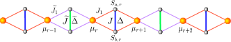
Figure 1: (Color online) A fragment from the Ising-$XXZ$ diamond chain with two impurities. The Ising spins is denoted by $\mu_{r}$, while $S_{a,r}$ are the Heisenberg spins.

Let us consider the Ising-$XXZ$ model with two impurities on a diamond chain in the presence of an external magnetic field. The various interaction parameters $\left(J,\Delta,J_{1}\right)$ are homogeneous along the diamond chain, except in the impurities where the corresponding parameters $\left(\widetilde{J},\widetilde{\Delta},\widetilde{J}_{1}\right)$ are different as shown in the Fig. 1. The Ising-$XXZ$ model consist of the Ising spins $\mu_{i}$ locate at the nodal lattice sites as well as, interstitial Heisenberg spins $S_{a(b)}^{\alpha}(\alpha=x,y,z)$.

Thus, the total hamiltonian for the Ising-$XXZ$ diamond chain with two impurities embedded in the model is given by $\mathcal{H}=\sum_{i=1}^{N}\mathcal{H}_{i}$, where

$$\mathcal{H}_{i}=\mathcal{H}_{i}^{host}+\mathcal{H}_{i}^{imp}+\mathcal{H}_{i}^{iso},$$

and

$$\begin{array}[]{cl}\mathcal{H}_{i}^{host}=&J\left(\mathbf{S}_{a,i},\mathbf{S}_{b,i}\right)_{\Delta}+J_{1}\left(S_{a,i}^{z}+S_{b,i}^{z}\right)\left(\mu_{i}+\mu_{i+1}\right)\\ &-h\left(S_{a,i}^{z}+S_{b,i}^{z}\right)-\frac{h}{2}\left(\mu_{i}+\mu_{i+1}\right),\\ &\mathrm{for}\>i=1,2,\ldots,r-2,r+2,\ldots,N\end{array}$$

is the hamiltonian of the host chain with $(\mathbf{S}_{a,i},\>\mathbf{S}_{b,i})_{\Delta}=(S_{a,i}^{x}S_{b,i}^{x}+S_{a,i}^{y}S_{b,i}^{y}+\Delta S_{a,i}^{z}S_{b,i}^{z})$ and $\mu_{i}=\pm 1/2$.

Whereas

$$\begin{array}[]{cl}\mathcal{H}_{i}^{imp}=&\widetilde{J}\left(\mathbf{S}_{a,i},\mathbf{S}_{b,i}\right)_{\widetilde{\Delta}}+\widetilde{J}_{1}\left(S_{a,i}^{z}+S_{b,i}^{z}\right)\left(\mu_{i}+\mu_{i+1}\right)\\ &-h\left(S_{a,i}^{z}+S_{b,i}^{z}\right)-\frac{h}{2}\left(\mu_{i}+\mu_{i+1}\right),\\ &\mathrm{for}\>i=r-1,r+1\end{array}$$

is the hamiltonian of the impurities of the model. Finally,

$$\begin{array}[]{cl}\mathcal{H}_{i}^{iso}=&J\left(\mathbf{S}_{a,i},\mathbf{S}_{b,i}\right)_{\Delta}+J_{1}\left(S_{a,i}^{z}+S_{b,i}^{z}\right)\left(\mu_{i}+\mu_{i+1}\right)\\ &-h\left(S_{a,i}^{z}+S_{b,i}^{z}\right)-\frac{h}{2}\left(\mu_{i}+\mu_{i+1}\right)\\ &\mathrm{for}\>i=r\end{array}$$

is the hamiltonian of the plaquette isolated in between of the impurities.

Here, $J$ and $\Delta$ denote the $XXZ$ interaction within the interstitial Heisenberg dimers, while $J_{1}$ label the interactions between the nodal Ising spins and interstitial Heisenberg spins, and the quantities $\widetilde{J}=J\left(1+\alpha\right)$, $\widetilde{\Delta}=\Delta\left(1+\gamma\right)$ and $\widetilde{J}_{1}=J_{1}\left(1+\eta\right)$ are defined analogously for the impurities. In addition $\alpha$, $\gamma$ and $\eta$ measures the strength of the impurities. Finally, $h$ is the magnetic field along the $z$-axis.

After straightforward calculation, the eigenvalues for the host hamiltonian $\mathcal{H}_{i}^{host}$ can be written as

$$\mathcal{\varepsilon}_{i1,i4}= \frac{J\Delta}{4}\pm\left(J_{1}\mp\frac{h}{2}\right)(\mu_{i}+\mu_{i+1})\mp\frac{h}{2},$$

$$\mathcal{\varepsilon}_{i2,i3}= -\frac{J\Delta}{4}\pm\frac{J}{2}-\frac{h}{2}(\mu_{i}+\mu_{i+1}),$$

where their corresponding eigenstate in terms of standard basis $\{|00\rangle,|01\rangle,|10\rangle,|11\rangle\}$ are given respectively by

$$|\varphi_{i1}\rangle= |00\rangle_{i},$$ (1)

$$|\varphi_{i2}\rangle= \frac{1}{\sqrt{2}}\left(|01\rangle_{i}+|10\rangle_{i}\right),$$ (2)

$$|\varphi_{i3}\rangle= \frac{1}{\sqrt{2}}\left(|01\rangle_{i}-|10\rangle_{i}\right),$$ (3)

$$|\varphi_{i4}\rangle= |11\rangle_{i}.$$ (4)

On the other hand, the eigenvalues of the impurity hamiltonian $\mathcal{H}_{i}^{imp}$ is given by

$$\begin{array}[]{cl}\mathcal{\epsilon}_{i1,i4}=&\frac{\widetilde{J}\widetilde{\Delta}}{4}\pm\left(\widetilde{J}_{1}\mp\frac{h}{2}\right)(\mu_{i}+\mu_{i+1})\mp\frac{h}{2},\\ \mathcal{\epsilon}_{i2,i3}=&-\frac{\widetilde{J}\widetilde{\Delta}}{4}\pm\frac{\widetilde{J}}{2}-\frac{h}{2}(\mu_{i}+\mu_{i+1}),\end{array}$$

with corresponding eigenvectors

$$\begin{array}[]{cl}|\widetilde{\varphi}_{i1}\rangle=&|00\rangle_{i},\\ |\widetilde{\varphi}_{i2}\rangle=&\frac{1}{\sqrt{2}}\left(|01\rangle_{i}+|10\rangle_{i}\right),\\ |\widetilde{\varphi}_{i3}\rangle=&\frac{1}{\sqrt{2}}\left(|01\rangle_{i}+|10\rangle_{i}\right),\\ |\widetilde{\varphi}_{i4}\rangle=&|11\rangle_{i},\end{array}$$

here $i=r-1$ and $i=r+1$. The spectrum shown above allows us to construct the partition function of the Ising-Heisenberg spin chain.

III The partition function and density operator

In order to measure the thermal entanglement, we first need to obtain a partition function on a diamond chain. Our model can be solved exactly using decoration transformation and transfer-matrix approach baxter . In this approach we will define the following operator as a function of Ising spin particles $\mu_{i}$ and $\mu_{i+1}$,

$$\varrho(\mu_{i},\mu_{i+1})=\sum_{j=1}^{4}\mathrm{e}^{-\beta\varepsilon_{ij}(\mu_{i},\mu_{i+1})}|\varphi_{ij}\rangle\langle\varphi_{ij}|,$$ (5)

where $\beta=1/k_{B}T$ with the Boltmann’s constant $k_{B}$ and $T$ is the absolute temperature.

Straightforwardly, we can obtain the Boltzmann factor by tracing out over the two-qubit operator,

$$w(\mu_{i},\mu_{i+1})=\mathrm{tr}_{ab}\left(\varrho(\mu_{i},\mu_{i+1})\right)=\sum_{j=1}^{4}\mathrm{e}^{-\beta\varepsilon_{ij}(\mu_{i},\mu_{i+1})},$$ (6)

and Boltzmann factor for impurity is given by

$$\widetilde{w}(\mu_{i},\mu_{i+1})=\sum_{j=1}^{4}\mathrm{e}^{-\beta\epsilon_{ij}(\mu_{i},\mu_{i+1})},$$

where $i=r-1$ and $i=r+1$.

The canonical partition function of the Ising-$XXZ$ diamond chain with two impurities can be written in terms of Boltzmann factors through the relation

$$Z_{N}= \sum_{\{\mu\}}w(\mu_{1},\mu_{2})\ldots\widetilde{w}(\mu_{r-1},\mu_{r})w(\mu_{r},\mu_{r+1})\times$$

$$\widetilde{w}(\mu_{r+1},\mu_{r+2})\ldots w(\mu_{N},\mu_{1}).$$ (7)

Using the transfer-matrix notation, we can write the partition function of the diamond chain straightforwardly by $Z_{N}=\mathrm{tr}\left(\widetilde{W}W\widetilde{W}W^{N-3}\right)$, where the transfer-matrix takes the following form

$$W=\left[\begin{array}[]{cc}w(\frac{1}{2},\frac{1}{2})&w(\frac{1}{2},-\frac{1}{2})\\ w(-\frac{1}{2},\frac{1}{2})&w(-\frac{1}{2},-\frac{1}{2})\end{array}\right].$$ (8)

Similarly for impurities, we have

$$\widetilde{W}=\left[\begin{array}[]{cc}\widetilde{w}(\frac{1}{2},\frac{1}{2})&\widetilde{w}(\frac{1}{2},-\frac{1}{2})\\ \widetilde{w}(-\frac{1}{2},\frac{1}{2})&\widetilde{w}(-\frac{1}{2},-\frac{1}{2})\end{array}\right].$$

The transfer matrix elements are denoted by $w_{++}\equiv w(\frac{1}{2},\frac{1}{2})$, $w_{+-}\equiv w(\frac{1}{2},-\frac{1}{2})$, $w_{--}\equiv w(-\frac{1}{2},-\frac{1}{2})$ and $\widetilde{w}_{++}\equiv\widetilde{w}(\frac{1}{2},\frac{1}{2})$, $\widetilde{w}_{+-}\equiv\widetilde{w}(\frac{1}{2},-\frac{1}{2})$, $\widetilde{w}_{--}\equiv\widetilde{w}(-\frac{1}{2},-\frac{1}{2})$.

The diagonalization of the transfer matrix (8), will provide the followings eigenvalues

$$\Lambda_{\pm}=\frac{w_{++}+w_{--}\pm Q}{2},$$ (9)

assuming that $Q=\sqrt{\left(w_{++}-w_{--}\right)^{2}+4w_{+-}^{2}}$. Therefore, the partition function for finite chain under periodic boundary conditions is given by

$$Z_{N}=A\Lambda_{+}^{N-3}+D\Lambda_{-}^{N-3},$$ (10)

where $A=a_{+}^{2}\Lambda_{+}+b_{+}b_{-}\Lambda_{-},$ $D=a_{-}^{2}\Lambda_{-}+b_{+}b_{-}\Lambda_{+}$ and

$$\begin{array}[]{cc}a_{\pm}=&\frac{\pm 4w_{+-}\widetilde{w}_{+-}\pm\left(w_{++}-w_{--}\right)\left(\widetilde{w}_{++}-\widetilde{w}_{--}\right)+Q\left(\widetilde{w}_{++}+\widetilde{w}_{--}\right)}{2Q}\\ b_{\pm}=&\frac{\left(w_{++}-w_{--}\pm Q\right)\left[\mp\left(\widetilde{w}_{++}-\widetilde{w}_{--}\right)\pm\widetilde{w}_{+-}\left(w_{++}-w_{--}\right)\right]}{2Qw_{+-}}.\end{array}$$

In the thermodynamic limit ($N\rightarrow\infty$) the partition function will be simplified, which results in

$$Z_{N}=A\Lambda_{+}^{N-3}.$$

III.1 Average reduced density operator

In order to calculate the average reduced density operator $\rho$, we will use the two-qubit Heisenberg operator $\varrho$, the matrix representation of this two-qubit operator is given by

$$\varrho(\mu_{i},\mu_{i+1})=\left[\begin{array}[]{cccc}\varrho_{1,1}&0&0&0\\ 0&\varrho_{2,2}&\varrho_{2,3}&0\\ 0&\varrho_{3,2}&\varrho_{3,3}&0\\ 0&0&0&\varrho_{4,4}\end{array}\right],$$ (11)

where

$$\varrho_{1,1}(\mu_{i},\mu_{i+1})= \mathrm{e}^{-\beta\varepsilon_{i1}(\mu_{i},\mu_{i+1})},$$

$$\varrho_{2,2}(\mu_{i},\mu_{i+1})= \frac{1}{2}\left(\mathrm{e}^{-\beta\varepsilon_{i2}(\mu_{i},\mu_{i+1})}+\mathrm{e}^{-\beta\varepsilon_{i3}(\mu_{1},\mu_{i+1})}\right),$$

$$\varrho_{2,3}(\mu_{i},\mu_{i+1})= \frac{1}{2}\left(\mathrm{e}^{-\beta\varepsilon_{i2}(\mu_{i},\mu_{i+1})}-\mathrm{e}^{-\beta\varepsilon_{i3}(\mu_{i},\mu_{i+1})}\right),$$

$$\varrho_{4,4}(\mu_{i},\mu_{i+1})= \mathrm{e}^{-\beta\varepsilon_{i4}(\mu_{i},\mu_{i+1})}.$$ (12)

In order to investigate the thermal entanglement for the system, we will perform the reduced density operator bounded by Ising particles along a diamond chain. In particularly, we focus in the average reduced density operator for the isolated two-qubit Heisenberg located between the impurities. The reduced density matrix elements can be written as

$$\rho_{k,l}= \frac{1}{Z_{N}}\sum_{\{\mu\}}w(\mu_{1},\mu_{2})\ldots\widetilde{w}(\mu_{r-1},\mu_{r})\varrho_{k,l}(\mu_{r},\mu_{r+1})\times$$

$$\widetilde{w}(\mu_{r+1},\mu_{r+2})\ldots w(\mu_{N},\mu_{1}).$$ (13)

Using the transfer-matrix notation, the elements can be alternatively rewritten as

$$\begin{array}[]{rl}\rho_{k,l}=&\frac{1}{Z_{N}}tr\left(W^{r-2}\widetilde{W}P_{k,l}\widetilde{W}W^{N-r-1}\right)\\ =&\frac{1}{Z_{N}}tr\left(\widetilde{W}P_{k,l}\widetilde{W}W^{N-3}\right),\end{array}$$

where

$$P_{k,l}=\left[\begin{array}[]{cc}\varrho_{k,l}(++)&\varrho_{k,l}(+,-)\\ \varrho_{k,l}(-,+)&\varrho_{k,l}(-,-)\end{array}\right],$$ (14)

and $\varrho_{k,l}(++)\equiv\varrho_{k,l}(\tfrac{1}{2},\tfrac{1}{2})$, $\varrho_{k,l}(+-)\equiv\varrho_{k,l}(\tfrac{1}{2},-\tfrac{1}{2})$, $\varrho_{k,l}(-+)\equiv\varrho_{k,l}(-\tfrac{1}{2},\tfrac{1}{2})$, $\varrho_{k,l}(--)\equiv\varrho_{k,l}(-\tfrac{1}{2},-\tfrac{1}{2})$.

The corresponding matrix $U$ that diagonalizes the transfer matrix $W$ can be given by

$$U=\left[\begin{array}[]{cc}\Lambda_{+}-w_{--}&\Lambda_{-}-w_{--}\\ w_{+-}&w_{+-}\end{array}\right],$$ (17)

and

$$U^{-1}=\left[\begin{array}[]{cc}\frac{1}{Q}&-\frac{\Lambda_{-}-w_{--}}{Qw_{+-}}\\ -\frac{1}{Q}&\frac{\Lambda_{+}-w_{--}}{Qw_{+-}}\end{array}\right].$$ (20)

Finally, the individual matrix elements of the averaged reduced density operator for the isolated dimer between two impurities defined in Eq.(13) must be expressed by

$$\rho_{k,l}=\tfrac{\mathrm{tr}\left(U^{-1}\widetilde{W}P_{k,l}\widetilde{W}U\left[\begin{smallmatrix}\Lambda_{+}^{N-3}&0\\ 0&\Lambda_{-}^{N-3}\end{smallmatrix}\right]\right)}{A\Lambda_{+}^{N-3}+D\Lambda_{-}^{N-3}}.$$ (21)

This result is valid for arbitrary number $N$ of cells in a diamond chain.

In the thermodynamic limit ($N\rightarrow\infty$) and assuming $\left(\Lambda_{-}/\Lambda_{+}\right)^{N}\rightarrow 0$ in this limit, the reduced density operator elements after a cumbersome algebra, is given by

$$\rho_{k,l}= \frac{1}{A}\left\{a_{+}^{2}\mathcal{M}_{k,l}^{+}+a_{+}b_{+}\mathcal{N}_{k,l}^{-}+a_{+}b_{-}\mathcal{N}_{k,l}^{+}+b_{+}b_{-}\mathcal{M}_{k,l}^{-}\right\},$$

where

$$\begin{array}[]{cl}\mathcal{M}_{k,l}^{\pm}=&\frac{\left(\varrho_{k,l}(++)+\varrho_{k,l}(--)\right)}{2}\pm\frac{2w_{+-}\varrho_{k,l}(+-)}{Q}\\ &\pm\frac{\left(\varrho_{k,l}(++)-\varrho_{k,l}(--)\right)\left(w_{++}-w_{--}\right)}{2Q},\end{array}$$

$$\begin{array}[]{cl}\mathcal{N}_{k,l}^{\pm}=&\frac{\left[\mp(\varrho_{k,l}(++)-\varrho_{k,l}(--))w_{+-}\pm\varrho_{k,l}(--)(w_{++}-w_{--})\right]}{2Qw_{+-}}\times\\ &\left(w_{++}-w_{--}\pm Q\right).\end{array}$$

All elements of average reduced density operator of the dimer immerse between two impurities of the diamond structure can be written as

$$\rho=\left[\begin{array}[]{cccc}\rho_{1,1}&0&0&0\\ 0&\rho_{2,2}&\rho_{2,3}&0\\ 0&\rho_{3,2}&\rho_{3,3}&0\\ 0&0&0&\rho_{4,4}\end{array}\right].$$ (22)

Next, let us calculate the thermal entanglement behaviour of the dimer Heisenberg isolated between two impurities.

IV Thermal entanglement of two-qubit Heisenberg between two impurities

In order to quantifying the thermal entanglement of the Heisenberg qubits isolated in middle of the two impurities embedded in the Ising-$XXZ$ diamond chain (see Fig. 1), we use the concurrence $\mathcal{C}$ define by Wootters woo .

$$\mathcal{C}(\rho)=\mathrm{max}\{0,\sqrt{\lambda_{1}}-\sqrt{\lambda_{2}}-\sqrt{\lambda_{3}}-\sqrt{\lambda_{4}}\},$$ (23)

where $\lambda_{i}$ are eigenvalues in decreasing order of matrix $R$,

$$R=\rho\cdot\left(\sigma^{y}\otimes\sigma^{y}\right)\cdot\rho^{*}\cdot\left(\sigma^{y}\otimes\sigma^{y}\right),$$ (24)

which is constructed as a function of the density operator $\rho$ given by Eq. (22), with the asterisk denoting the complex conjugate of matrix $\rho$.

Thereafter, after a short algebra, the corresponding concurrence for our system can be reduced to

$$\mathcal{C}(\rho)=2\mathrm{max}\{0,|\rho_{2,3}|-\sqrt{\rho_{1,1}\rho_{4,4}}\}.$$ (25)

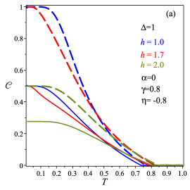
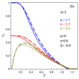
Figure 2: The concurrence as a function of temperature $T$ for different values of the magnetic field, with $J_{1}/J=1$. In this figure we consider the original model without impurities (solid line). On the other hand, for the model with impurities (dashed line), we consider the parameters $\alpha=0$, $\gamma=0.8$, $\eta=-0.8$. (a) $\Delta=1.0$; (b) $\Delta=2$.

The thermal entanglement properties for Ising-$XXZ$ diamond chain structure have been investigated in Reference moi . Here we are mainly concerned about the effects on the thermal entanglement caused by the impurities in the Ising-$XXZ$ diamond chain. More specifically, let us focus on the thermal entanglement of the isolated two-qubit Heisenberg (dimer) located between the impurities.

From now on, we will plot the curves of the original model with solid lines, while for the Ising-$XXZ$ diamond chain with two impurities, we will use dashed lines.

In Fig. 2 we describe the behavior of the concurrence $\mathcal{C}$ with respect of the temperature $T$ for different values of the magnetic field $h$ and impurities parameters $\alpha=0$, $\gamma=0.8$ and $\eta=-0.8$. In Fig. 2(a), we observed a dramatic increase in the concurrence when the model has impurities. From this figure, it can be clearly seen that, for the Ising-$XXZ$ diamond chain with two anisotropic impurities $(\widetilde{\Delta}=1.8)$, the concurrence increases strongly, reaching the maximum entanglement (see dashed line) for different values of the magnetic field. On the other hand, in Fig. 2(b) we can see that for high values of the anisotropy ($\Delta=2$ and $\widetilde{\Delta}=2.8$) the effect of the impurities are weak, whereas for the temperatures $T=0$ and $T\apprge 1.1$ the effects of impurities are null.

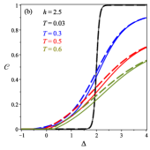
Figure 3: (Color online) The concurrence as a function of the anisotropy factor $\Delta$ for different values of the temperature $T$, with $J_{1}/J=1$. For the Ising-$XXZ$ model without impurities we have $\alpha=\gamma=\eta=0$ (solid line). On the other hand, for the model with impurities, we fixed $\alpha=0$, $\gamma=0.8$ and $\eta=-0.8$ (dashed line). (a) $h=1.2$; (b) $h=2.5$.

In Fig. 3, the concurrence $\mathcal{C}$ is plotted as a function of anisotropy parameter $\Delta$ for different values of the temperature and the fixed values of impurities parameters $\alpha=0$, $\gamma=0.8$ and $\eta=-0.8$. We can observe in these figures that, for ${\color[rgb]{0,0,0}h=1.2}$ and ${\color[rgb]{0,0,0}h=2.5}$ we have transition from unentangled ferrimagnetic (${\color[rgb]{0,0,0}UFI}$) to entangled state (${\color[rgb]{0,0,0}ENQ}$) and unentagled ferromagnetic state (${\color[rgb]{0,0,0}UFM}$) to same entanglement state (${\color[rgb]{0,0,0}ENQ}$) respectively (see moi ). As one can see from Fig. 3(a) the anisotropic behavior of the thermal concurrence for impurities is more robust. We can also observe that the presence of impurities will allow the existence of thermal entanglement in regions beyond the reach of the original model. In Fig. 3(b), we can see that, for strong magnetic fields and low temperatures, the effect of impurity disappears are gradually lost. Now, when we increase the temperature, the thermal entanglement it is slightly more robust in the presence of impurities. We can conclude that the entanglement for the model with impurities is much more intense than the model without impurities in a broader range of the anisotropy parameter.

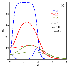
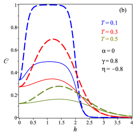
Figure 4: (Color online) The concurrence as a function of the magnetic field $h$, for $J_{1}/J=1$ and different values of the temperature $T$. (a) $\Delta=0.9$; (b) $\Delta=1$.

In Fig. 4, the variations of concurrence $\mathcal{C}$ with magnetic field $h$ for different values of temperature $T$ and fixed values of the impurities parameter $\alpha=0$, $\gamma=0.8$ and $\eta=-0.8$ are plotted in two different cases (i.e $\Delta=0.9$ and $\Delta=1$). In Fig. 4 (a), the curve for $T=0.1$ on original model becomes unentangled in the interval $0.6\apprle h\apprle 1.4.$ In contrast, in our model with impurities this is maximally entangled, signaling the strong influence of impurities in the entanglement of the our model. Similar behavior has the concurrence when the temperature increases. Thus, from this figure, we can see that for $T=0.3$, the concurrence reaches the value $\mathcal{C}\mathit{\approx\mathrm{0.24}}$ for the original model, while for model with impurities we obtain $\mathcal{C}\mathit{\approx}0.65$. While, for $T=0.5$, we obtain $\mathcal{C}\mathit{\approx}0.13$ in the original model, already in the model with impurities we obtained $\mathcal{C}\mathit{\approx\mathrm{0.24}}$. In Fig. 4 (b) we can see the enhancing the concurrence (dashed line) when compared to the model without impurities (solid line). Thus, in low temperature $T=0.1$, we have a sudden increase the concurrence until $\mathcal{C}\mathit{=\mathrm{1}}$ for the model with impurities. However, for the model without impurities we obtained $\mathcal{C}\mathit{=\mathrm{0.5}}$. Moreover, it can be observed in this figure that, for higher temperatures (e.g $T=0.3$, $T=0.5$), the entanglement is still greater than in the case without impurities. We also observed that, for intense magnetic fields, the effect of the impurities no longer influences in entanglement.

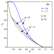
Figure 5: (Color online) The concurrence versus temperature for different values of the magnetic field $h=1.6$ (blue), $h=2.4$ (green), $J=J_{1}=1$, $\Delta=2$. The concurrence of the model with impurity is show in dashed line. (a) $\eta=-1$ (dashed line); (b) $\alpha=-1$ (dashed line).

Finally, in Fig. 5 let us study the behavior of the system in two extreme cases. In Fig. 5 (a), we analyze the case when $\widetilde{J}_{1}=0$ or $\eta=-1$ which corresponds to the collapse of Ising-like interaction of the impurities with the dimer isolated from diamond chain. We observed that we can enhanced the concurrence of the dimer located between the impurities when it is isolated from the diamond chain. Is notable that the entanglement can be changed by the presence of impurities even in the case where the physical coupling (Ising type) to the impurity is null. On the other hand, in Fig. 5 (b) let us consider $\widetilde{J}=0$ or $\alpha=-1$, this case corresponds to the situation where the Heisenberg interaction in the impurities is null. It easily can be seen that the thermal concurrence decreases in the dimer located between the impurities.

V Conclusions

In summary, in this paper we investigated the effects of the impurities local sites on the Ising-${\color[rgb]{0,0,0}XXZ}$ diamond chain. In the model we have two impurities with an isolated $XXZ$ dimer between them. In particular, we have developed a method to solve exactly the Ising-$XXZ$ diamond chain with two impurities. Our attention has been focused on the study the thermal entanglement of the isolated $XXZ$ dimer. We demonstrate, that the thermal entanglement can be controlled and tuned by introducing impurities into an Ising-$XXZ$ chain.

As a matter of fact, for certain parameters of the impurities, the thermal entanglement is maximum in low temperatures, unlike what happens in the model without impurities. On the other hand, for high temperatures, the effects of the impurities is null. Moreover, the concurrence have been examined in detail with respect to the anisotropy parameter, we observed that impurities strongly influence at the behavior of the entanglement at low temperatures for weak magnetic fields. More specifically, the results showns the existence of thermal entanglement in regions beyond the reach of the original model. While, for strong magnetic fields the effect of anisotropy on entanglement is very weak. Similar behavior is obtained for entanglement as a function of the magnetic field. For weak magnetic fields, the model is maximally entanglement in contrast to the same model without impurities. However, for strong magnetic fields, impurities have no more influence in the thermal entanglement for both models. Furthermore, our results sheds some light on the local control of thermal entanglement by manipulating the parameters of the impurities inserted in the Ising-$XXZ$ diamond chain. Finally, it is expected that this new approach may be helpful for realising the quantum teleportation process of information.

References

- (1) C. H. Bennett and D. P. DiVincenzo, Nature. 404, 247 (2000); C. H. Bennett and S. J. Wiesner, Phys. Rev. Lett. 69, 2881 (1992); A. K. Ekert . 67, 661 (1991); A. Zeilinger Phys. Scripta T76, 203 (1998).
- (2) D. Loss and D. P. DiVincenzo, Phys. Rev. A 57, 120 (1998).
- (3) G. L. Kamta, A. F. Starace, Phys. Rev. Lett. 88, 107901 (2002); S. L. Zhu, Phys. Rev. Lett. 96, 077206 (2006).
- (4) G. F. Zhang, S. S. Li, Phys. Rev. A 72, 034302 (2005).
- (5) M. C. Arnesen, S. Bose, V. Vedral, Phys. Rev. Lett. 87, 017901 (2001).
- (6) X. G. Wang, Phys. Rev. A 64, 012313 (2001).
- (7) L. Canova, J. Strecka, M. Jascur, J. Phys: Condens. Matter 18, 4967 (2006).
- (8) B. Lisnyi and J. Strecka, Phys. Status Solidi B 251, 1083 (2014).
- (9) O. Rojas, M. Rojas, N. S. Ananikian, and S. M de Souza, Phys. Rev. A 86, 042330 (2012).
- (10) J. Torrico, M. Rojas, S. M. de Souza, O. Rojas and N. S. Ananikian, Europhys. Lett. 108, 50007 (2014).
- (11) V. S. Abgaryan. N. S. Ananikian, L. N. Ananikian and V. Hovhannisyan, Solid State Commun. 203, 5 (2015).
- (12) M. Rojas, S. M. de Souza and Onofre Rojas, Ann. Phys. 377, 506 (2017).
- (13) W. W. Cheng, X. Y. Wang, Y. B. Sheng, L. Y. Gong, S. M. Yhao, J. M. Liu, Sci. Rep. 7, 42360 (2017).
- (14) H. Falk, Phys Rev. 151, 304 (1966).
- (15) J. Stolke, M. Vogel, Phys. Rev. B 61, 4026 (2000).
- (16) Xiaoguang Wang, Phys. Rev. E 69, 066118 (2004).
- (17) X. Huang, Z. Yang, J. Magn. Magn. Mater. 381, 372 (2015).
- (18) Y. Sun, X. Huang, G. Min, Phys. Lett. A 381, 387 (2017).
- (19) O. Osenda, Z. Huang, S. Kais, Phys. Rev. A 67, 062321 (2003).
- (20) H. Fu, A. I. Salomon, X. Wang, J. Phys. A 35, 4293 (2002).
- (21) Jia-Min Gong, Zhan-Qiang Hui, Physica B 444, 40 (2014).
- (22) R. J. Baxter, , Academic, New York, 1982.
- (23) K. Wootters, Phys. Rev. Lett. 80, 2248 (1998).