Abstract
Word vector representations are well developed tools for various NLP and Machine Learning tasks and are known to retain significant semantic and syntactic structure of languages. But they are prone to carrying and amplifying bias which can perpetrate discrimination in various applications. In this work, we explore new simple ways to detect the most stereotypically gendered words in an embedding and remove the bias from them. We verify how names are masked carriers of gender bias and then use that as a tool to attenuate bias in embeddings. Further, we extend this property of names to show how names can be used to detect other types of bias in the embeddings such as bias based on race, ethnicity, and age.
Attenuating Bias in Word Vectors
Sunipa Dev Jeff Phillips
University of Utah University of Utah
1 BIAS IN WORD VECTORS
Word embeddings are an increasingly popular application of neural networks wherein enormous text corpora are taken as input and words therein are mapped to a vector in some high dimensional space. Two commonly used approaches to implement this are WordToVec [16, 15] and GloVe [17]. These word vector representations estimate similarity between words based on the context of their nearby text, or to predict the likelihood of seeing words in the context of another. Richer properties were discovered such as synonym similarity, linear word relationships, and analogies such as man : woman :: king : queen. Their use is now standard in training complex language models.
However, it has been observed that word embeddings are prone to express the bias inherent in the data it is extracted from [3, 4, 7]. Further, Zhao et al. (2017) [18] and Hendricks et al. (2018) [6] show that machine learning algorithms and their output show more bias than the data they are generated from.
Word vector embeddings as used in machine learning towards applications which significantly affect people’s lives, such as to assess credit [11], predict crime [5], and other emerging domains such judging loan applications and resumes for jobs or college applications. So it is paramount that efforts are made to identify and if possible to remove bias inherent in them. Or at least, we should attempt minimize the propagation of bias within them. For instance, in using existing word embeddings, Bolukbasi et al. (2016) [3] demonstrated that women and men are associated with different professions, with men associated with leaderships roles and professions like doctor, programmer and women closer to professions like receptionist or nurse. Caliskan et al. (2017) [7] similarly noted how word embeddings show that women are more closely associated with arts than math while it is the opposite for men. They also showed how positive and negative connotations are associated with European-American versus African-American names.
Our work simplifies, quantifies, and fine-tunes these approaches: we show that very simple linear projection of all words based on vectors captured by common names is an effective and general way to significantly reduce bias in word embeddings. More specifically:
-
1a.
We demonstrate that simple linear projection of all word vectors along a bias direction is more effective than the Hard Debiasing of Bolukbasi et al. (2016) [3] which is more complex and also partially relies on crowd sourcing.
-
1b.
We show that these results can be slightly improved by dampening the projection of words which are far from the projection distance.
-
2.
We examine the bias inherent in the standard word pairs used for debiasing based on gender by randomly flipping or swapping these words in the raw text before creating the embeddings. We show that this alone does not eliminate bias in word embeddings, corroborating that simple language modification is not as effective as repairing the word embeddings themselves.
-
3a.
We show that common names with gender association (e.g., john, amy) often provides a more effective gender subspace to debias along than using gendered words (e.g., he, she).
-
3b.
We demonstrate that names carry other inherent, and sometimes unfavorable, biases associated with race, nationality, and age, which also corresponds with bias subspaces in word embeddings. And that it is effective to use common names to establish these bias directions and remove this bias from word embeddings.
2 DATA AND NOTATIONS
We set as default the text corpus of a Wikipedia dump (dumps.wikimedia.org/enwiki/latest/enwiki-latest-pages-articles.xml.bz2) with 4.57 billion tokens and we extract a GloVe embedding from it in dimensions per word. We restrict the word vocabulary to the most frequent words. We also modify the text corpus and extract embeddings from it as described later.
So, for each word in the Vocabulary , we represent the word by the vector in the embedding. The bias (e.g., gender) subspace is denoted by a set of vector . It is typically considered in this work to be a single unit vector, (explained in detail later). As we will revisit, a single vector is typically sufficient, and will simplify descriptions. However, these approaches can be generalized to a set of vectors defining a multi-dimensional subspace.
3 HOW TO ATTENUATE BIAS
Given a word embedding, debiasing typically takes as input a set of equality sets. An equality set for instance can be a single pair (e.g., {man, woman}), but could be more words (e.g., {latina, latino, latinx}) that if the bias connotation (e.g, gender) is removed, then it would objectively make sense for all of them to be equal. Our data sets will only use word pairs (as a default the ones in Table 1), and we will describe them as such hereafter for simpler descriptions. In particular, we will represent each as a set of two vectors .
Given such a set of equality sets, the bias vector can be formed as follows [3]. For each create a vector between the pairs. Stack these to form a matrix , and let be the top singular vector of . We revisit how to create such a bias direction in Section 4.
| {man,woman}, {son,daughter}, {he,she}, {his,her}, |
|---|
| {male,female}, {boy,girl}, {himself,herself}, |
| {guy,gal}, {father,mother}, {john,mary} |
Now given a word vector , we can project it to its component along this bias direction as
3.1 Existing Method : Hard Debiasing
The most notable advance towards debiasing embeddings along the gender direction has been by Bolukbasi et al. (2016) [3] in their algorithm called Hard Debiasing (). It takes a set of words desired to be neutralized, , a unit bias subspace vector , and a set of equality sets .
First, words are projected orthogonal to the bias direction and normalized
Second, it corrects the locations of the vectors in the equality sets. Let be the mean of an equality set, and be the mean of of equality set means. Let be the offset of a particular equality set from the mean. Now each in each equality set is first centered using their average and then neutralized as
Intuitively quantifies the amount words in each equality set differ from each other in directions apart from the gender direction. This is used to center the words in each of these sets.
This renders word pairs such as man and woman as equidistant from the neutral words with each word of the pair being centralized and moved to a position opposite the other in the space. This can filter out properties either word gained by being used in some other context, like mankind or humans for the word man.
The word set which is debiased is obtained in two steps. First it seeds some words as definitionally gendered via crowd sourcing and using dictionary definitions; the complement – ones not selected in this step – are set as neutral. Next, using this seeding an SVM is trained and used to predict among all the set of other biased or neutral words . This set is taken as desired to be neutral and is debiased. Thus not all words in the vocabulary are debiased in this procedure, only a select set chosen via crowd-sourcing and definitions, and its extrapolation. Also the word vectors in the equality sets are also handled separately. This makes this approach not a fully automatic way to debias the vector embedding.
3.2 Alternate and Simple Methods
We next present some simple alternatives to HD which are simple and fully automatic. These all assume a bias direction .
Subtraction. As a simple baseline, for all word vectors subtract the gender direction from :
Linear Projection. A better baseline is to project all words orthogonally to the bias vector .
This enforces that the updated set has no component along , and hence the resulting span is only dimensions. Reducing the total dimension from say to should have minimal effects of expressiveness or generalizability of the word vector embeddings.
Bolukbasi et al. [3] apply this same step to a dictionary definition based extrapolation and crowd-source-chosen set of word pairs . We quantify in Section 5 that this single universal projection step debiases better than HD.
For example, consider the bias as gender, and the equality set with words man and woman. Linear projection will subtract from their word embeddings the proportion that were along the gender direction learned from a larger set of equality pairs. It will make them close-by but not exactly equal. The word man is used in many extra senses than the word woman; it is used to refer to humankind, to a person in general, and in expressions like “oh man”. In contrast a simpler word pair with fewer word senses, like (he - she) and (him - her), we can expect them to be almost at identical positions in the vector space after debiasing, implying their synonymity.
Thus, this approach uniformly reduces the component of the word along the bias direction without compromising on the differences that words (and word pairs) have.
3.3 Partial Projection
A potential issue with the simple approaches is that they can significantly change some embedded words which are definitionally biased (e.g., the neutral words described by Bolukbasi et al. [3]). [[We note that this may not *actually* be a problem (see Section 5); the change may only be associated with the bias, so removing it would then not change the meaning of those words in any way except the ones we want to avoid.]] However, these intuitively should be words which have correlation with the bias vector, but also are far in the orthogonal direction. In this section we explore how to automatically attenuate the effect of the projection on these words.
This stems from the observation that given a bias direction, the words which are most extreme in this direction (have the largest dot product) sometimes have a reasonable biased context, but some do not. These “false positives” may be large normed vectors which also happen to have a component in the bias direction.
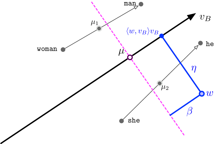
We start with a bias direction and mean derived from equality pairs (defined the same way as in context of HD). Now given a word vector we decompose it into key values along two components, illustrated in Figure 1. First, we write its bias component as
This is the difference of from when both are projected onto the bias direction .
Second, we write a (residual) orthogonal component
Let be its value. It is the orthogonal distance from the bias vector ; recall we chose to pass through the origin, so the choice of does not affect this distance.
Now we will maintain the orthogonal component (, which is in a subspace spanned by out of dimensions) but adjust the bias component to make it closer to . But the adjustment will depend on the magnitude . As a default we set
so all word vectors retain their orthogonal component, but have a fixed and constant bias term. This is functionally equivalent to the Linear Projection approach; the only difference is that instead of having a magnitude along (and the orthogonal part unchanged), it instead has a magnitude of constant along (and the orthogonal part still unchanged). This adds a constant to every inner product, and a constant offset to any linear projection or classifier. If we are required to work with normalize vectors (we do not recommend this as the vector length captures veracity information about its embedding), we can simple set .
Given this set-up, we now propose three modifications. In each set
were for is a function of only the orthogonal value . For the default case
Here is a hyperparameter that controls the importance of ; in Section 3.4 we show that we can just set . x
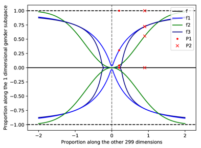
In Figure 2 we see the regions of the -space that the functions , and consider gendered. projects all points onto the line. But variants , , and are represented by curves that dampen the bias reduction to different degrees as increases. Points P1 and P2 have the same dot products with the bias direction but different dot products along the other dimensions. We can observe the effects of each dampening function as increases from P1 to P2.
3.4 SETTING .
To complete the damping functions , , and , we need a value . If is larger, then more word vectors have bias completely removed; if is smaller, than more words are unaffected by the projection. The goal is that words which are likely to carry a bias connotation to have little damping (small values) and words which are unlikely to carry a bias connotation to have more damping (large values – they are not moved much).
Given sets and , we can define a gain function
with a regularization term . The gain is large when most bias words in have very little damping (small , large ), and the opposite is true for the neutral words in . We want the neutral words to have large and hence small , so they do not change much.
To define the gain function, we need sets and ; we do so with the bias of interest as gender. The biased set is chosen among a set of popular names in which (based on babynamewizard.com and and SSN databases [2, 1]) are strongly associated with a gender. The neutral set is chosen as the most frequent words from , after filtering out obviously gendered words like names man and he. We also omit occupation words like doctor and others which may carry unintentional gender bias (these are words we would like to automatically de-bias). The neutral set may not be perfectly non-gendered, but it provides reasonable approximation of all non-gendered words.
We find for an array of choices for (we tried , , and ), the value approximately maximizes the gain function for each . So for hereafter we fix .
Although these sets and play a role somewhat similar to the crowd-sourced sets and from HD that we hoped to avoid, the role here is much reduced. This is just to verify that a choice of is reasonable, and otherwise they are not used.

3.5 Flipping the Raw Text
Since the embeddings preserve inner products of the data from which it is drawn, we explore if we can make the data itself gender unbiased and then observe how that change shows up in the embedding. Unbiasing a textual corpus completely can be very intricate and complicated since there are a many (sometimes implicit) gender indicators in text. Nonetheless, we propose a simple way of neutralizing bias in textual data by using word pairs ; in particular, when we observe in raw text on part of a word part, we randomly flip it to the other pair. For instance for gendered word pairs (e.g., (he - she)) in a string “he was a doctor” we may flip to “she was a doctor.”
We implement this procedure over the entire input raw text, and try various probabilities of flipping each observed word, focusing on probabilities , and . The first -flip probability makes each element of a word pair equally likely. The last -flip probability reverses the roles of those word pairs, and -flip probability does something in between. We perform this set of experiments on the default Wikipedia data set and switch between word pairs (say man woman, she he, etc), from a list larger that Table 3 consisting of 75 word pairs; see Supplementary Material D.1.
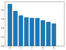
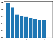
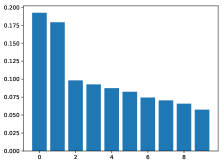
We observe how the proportion along the principal component changes with this flipping in Figure 3. We see that flipping with somewhat dampens the difference between the different principal components. On the other hand flipping with probability (and to a lesser extent ) exacerbates the gender components rather than dampening it. Now there are two components significantly larger than the others. This indicates this flipping is only addressing part of the explicit bias, but missing some implicit bias, and these effects are now muddled.
We list some gender biased analogies in the default embedding and how they change with each of the methods described in this section in Table 2.
| analogy head | original | HD | flipping | subtraction | projection | ||
|---|---|---|---|---|---|---|---|
| 0.5 | 0.75 | 1.0 | |||||
| man : woman :: doctor : | nurse | surgeon | dr | dr | medicine | physician | physician |
| man : woman :: footballer : | politician | striker | midfielder | goalkeeper | striker | politician | midfielder |
| he : she :: strong : | weak | stronger | weak | strongly | many | well | stronger |
| he : she :: captain : | mrs | lieutenant | lieutenant | colonel | colonel | lieutenant | lieutenant |
| john : mary :: doctor : | nurse | physician | medicine | surgeon | nurse | father | physician |
4 THE BIAS SUBSPACE
We explore ways of detecting and defining the bias subspace and recovering the most gendered words in the embedding. Recall as default, we use as the top singular vector of the matrix defined by stacking vectors of biased word pairs. We primarily focus on gendered bias, using words in Table 1, and show later how to effectively extend to other biases. We discuss this in detail in Supplementary Material C.
Most gendered words.
The dot product, of the word vectors with the gender subspace is a good indicator of how gendered a word is. The magnitude of the dot product tells us of the length along the gender subspace and the sign tells us whether it is more female or male. Some of the words denoted as most gendered are listed in Table 3.
| Gendered Words | |||
|---|---|---|---|
| miss | herself | forefather | himself |
| maid | heroine | nephew | congressman |
| motherhood | jessica | zahir | suceeded |
| adriana | seductive | him | sir |
| Female Adjectives | Male Adjectives |
|---|---|
| glamorous | strong |
| diva | muscular |
| shimmery | powerful |
| beautiful | fast |
| Female Occupations | Male Occupations |
|---|---|
| nurse | soldier |
| maid | captain |
| housewife | officer |
| prostitute | footballer |
4.1 Bias Direction using Names
When listing gendered words by , we observe that many gendered words are names. This indicates the potential to use names as an alternative (and potentially in a more general way) to bootstrap finding the gender direction.
From the top 100K words, we extract the 10 most common male and female names which are not used in ambiguous ways (e.g., not the name hope which could also refer to the sentiment). We pair these 10 names from each category (male, female) randomly and compute the SVD as before. We observe in 4 that the fractional singular values show a similar pattern as with the list of correctly gendered word pairs like (man - woman), (he - she), etc.


But this way of pairing names is quite imprecise. These names are not ‘opposites’ of each other in the sense that word pairs are. So, we modify how we compute now so that we can better use names to detect the bias in the embedding. The following method gives us this advantage where we do not necessarily need word pairs or equality sets as in Bolukbasi et al. [3].
Our gender direction is calculated as,
where and .
Using the default Wikipedia dataset, we found that this is a good approximator of the gender subspace defined by the first right singular vector calculated using gendered words from Table 1; there dot product is . We find similar large dot product scores for other datasets too.
Here too we collect all the most gendered words as per the gender direction determined by these names. Most gendered words returned are similar as using the default , like occupational words, adjectives, and synonyms for each gender. We find names to express similar classification of words along male - female vectors with homemaker more female and policeman being more male. We illustrate this in more detail in Table 4.
| Female Occ | Male Occ | Female* Occ | Male* Occ |
|---|---|---|---|
| nurse | captain | policeman | policeman |
| maid | cop | detective | cop |
| actress | boss | character | character |
| housewife | officer | cop | assassin |
| dancer | actor | assassin | bodyguard |
| nun | scientist | actor | waiter |
| waitress | gangster | waiter | actor |
| scientist | trucker | butler | detective |
Using that direction, we debias by linear projection. There is a similar shift in analogy results. We see a few examples in Table 5.
| analogy head | original | subtraction | projection |
|---|---|---|---|
| man : woman :: doctor : | nurse | physician | physician |
| man : woman :: footballer : | politician | politician | midfielder |
| he : she :: strong : | weak | very | stronger |
| he : she :: captain : | mrs | lieutenant | lieutenant |
| john : mary :: doctor : | nurse | dr | dr |
5 QUANTIFYING BIAS
In this section we develop new measures to quantify how much bias has been removed from an embedding, and evaluate the various techniques we have developed for doing so.
As one measure, we use the Word Embedding Association Test (WEAT) test developed by Caliskan et al. (2017) [7] as analogous to the IAT tests to evaluate the association of male and female gendered words with two categories of target words: career oriented words versus family oriented words. We detail WEAT and list the exact words used (as in [7]) in Supplementary Material B; smaller values are better.
Bolukbasi et al. [3] evaluated embedding bias use a crowsourced judgement of whether an analogy produced by an embedding is biased or not. Our goal was to avoid crowd sourcing, so we propose two more automatic tests to qualitatively and uniformly evaluate an embedding for the presence of gender bias.
Embedding Coherence Test (ECT).
A way to evaluate how the neutralization technique affects the embedding is to evaluate how the nearest neighbors change for (a) gendered pairs of words and (b) indirect-bias-affected words such as those associated with sports or occupational words (e.g., football, captain, doctor). We use the gendered word pairs in Table 1 for and the professions list as proposed and used by Bolukbasi et al. https://github.com/tolga-b/debiaswe (see also Supplementary Material D.2) to represent (b).
-
S1:
For all word pair we compute two means and . We find the cosine similarity of both and to all words . This creates two vectors .
-
S2:
We transform these similarity vectors to replace each coordinate by its rank order, and compute the Spearman Coefficient (in , larger is better) between the rank order of the similarities to words in .
Thus, here, we care about the order in which the words in occur as neighbors to each word pair rather than the exact distance. The exact distance between each word pair would depend on the usage of each word and thus on all the different dimensions other than the gender subspace too. But the order being relatively the same, as determined using Spearman Coefficient would indicate the dampening of bias in the gender direction (i.e., if doctor by profession is the 2nd closest of all professions to both man and woman, then the embedding has a dampened bias for the word doctor in the gender direction). Neutralization should ideally bring the Spearman coefficient towards 1.
Embedding Quality Test (EQT).
The demonstration by Bolukbasi et al. [3] about the skewed gender roles in embeddings using analogies is what we try to quantify in this test. We attempt to quantify the improvement in analogies with respect to bias in the embeddings.
We use the same sets and as in the ECT test. However, for each profession we create a list of their plurals and synonyms from WordNet on NLTK [14].
-
S1:
For each word pair , and each occupation word , we test if the analogy returns a word from . If yes, we set , and otherwise.
-
S2:
Return the average value across all combinations .
The scores for EQT are typically much smaller than for ECT. We explain two reasons for this.
First, EQT does not check for if the analogy makes relative sense, biased or otherwise. So, “man : woman :: doctor : nurse” is as wrong as “man : woman :: doctor : chair.” This pushes the score down.
Second, synonyms in each set as returned by WordNet [8] on the Natural Language Toolkit, NLTK [14] do not always contain all possible variants of the word. For example, the words psychiatrist and psychologist can be seen as analogous for our purposes here but linguistically are removed enough that WordNet does not put them as synonyms together. Hence, even after debiasing, if the analogy returns “man : woman :: psychiatrist : psychologist“ S1 returns 0. Further, since the data also has several misspelt words, archeologist is not recognized as a synonym or alternative for the word archaeologist. For this too S1 returns a 0.
The first caveat can be side-stepped by restricting the pool of words we search over for the analogous word to be from list . But it is debatable if an embedding should be penalized equally for returning both nurse or chair for the analogy “man : woman :: doctor : ?”
This measures the quality of analogies, with better quality having a score closer to .
| analogy head | original | HD | flipping | subtraction | projection | ||||
| 0.5 | 0.75 | 1.0 | word pairs | names | word pairs | names | |||
| ECT (word pairs) | 0.798 | 0.917 | 0.983 | 0.984 | 0.683 | 0.963 | 0.936 | 0.996 | 0.943 |
| ECT (names) | 0.832 | 0.968 | 0.714 | 0.662 | 0.587 | 0.923 | 0.966 | 0.935 | 0.999 |
| EQT | 0.128 | 0.145 | 0.131 | 0.098 | 0.085 | 0.268 | 0.236 | 0.283 | 0.291 |
| WEAT | 1.623 | 1.221 | 1.164 | 1.09 | 1.03 | 1.427 | 1.440 | 1.233 | 1.219 |
| WSim | 0.637 | 0.537 | 0.567 | 0.537 | 0.536 | 0.627 | 0.636 | 0.627 | 0.629 |
| Simlex | 0.324 | 0.314 | 0.317 | 0.314 | 0.264 | 0.302 | 0.312 | 0.321 | 0.321 |
| Google Analogy | 0.623 | 0.561 | 0.565 | 0.561 | 0.321 | 0.538 | 0.565 | 0.565 | 0.584 |
Evaluating embeddings.
We mainly run methods to evaluate our methods WEAT, EQT, and two variants of ECT: ECT (word pairs) uses defined by words in Table 1 and ECT (names) which uses vectors and derived by gendered names.
We observe in Table 6 that the ECT score increases for all methods in comparison to the non-debiased (the original) word embedding; the exception is flipping with probability score for ECT (word pairs) and all flipping variants for ECT (names). Flipping does nothing to affect the names, so it is not surprising that it does not improve this score; further indicating that it is challenging to directly fix bias in raw text before creating embeddings. Moreover, HD has the lowest score (of ) whereas projection obtains scores of (with ) and (with ).
EQT is a more challenging test, and the original embedding only achieves a score of , and HD only obtains (that is of occupation words have their related word as nearest neighbor). On the other hand, projection increases this percentage to (using ) and (using ). Even subtraction does nearly as well at between . Generally, the subtraction always performs slightly worse than projection.
For the WEAT test, the original data has a score of , and this is decreased the most by all forms of flipping, down to about . HD and projection do about the same with HD obtaining a score of and projection obtaining (with ) and (with ); values closer to 0 are better (See Supplementary Material B).
In the bottom of Table 6 we also run these approaches on standard similarity and analogy tests for evaluating the quality of embeddings. We use cosine similarity [13] on WordSimilarity-353 (WSim, 353 word pairs) [9] and SimLex-999 (Simlex, 999 word pairs) [10], each of which evaluates a Spearman coefficient (larger is better). We also use the Google Analogy Dataset using the function 3COSADD [12] which takes in three words which for a part of the analogy and returns the 4th word which fits the analogy the best.
We observe (as expected) that all that debiasing approaches reduce these scores. The largest decrease in scores (between and ) is almost always from HD. Flipping at rate is comparable to HD. And simple linear projection decreases the least (usually only about , except on analogies where it is (with ) or (with ).
In Table 7 we also evaluate the damping mechanisms defined by , , and , using . These are very comparable to simple linear projection (represented by ). The scores for ECT, EQT, and WEAT are all about the same as simple linear projection, usually slightly worse.
| Tests | f | |||
|---|---|---|---|---|
| ECT | 0.996 | 0.994 | 0.995 | 0.997 |
| EQT | 0.283 | 0.280 | 0.292 | 0.287 |
| WEAT | 1.233 | 1.253 | 1.245 | 1.241 |
| WSim | 0.627 | 0.628 | 0.627 | 0.627 |
| Simlex | 0.321 | 0.324 | 0.324 | 0.324 |
| Google Analogy | 0.565 | 0.571 | 0.569 | 0.569 |
While ECT, EQT and WEAT scores are in a similar range for all of , , , and ; the dampened approaches , , and performs better on the Google Analogy test. This test set is devoid of bias and is made up of syntactic and semantic analogies. So, a score closer to that of the original, biased embedding, tells us that more structure has been retained by , and . Overall, any of these approaches could be used if a user wants to debias while retaining as much structure as possible, but otherwise linear projection (or ) is roughly as good as these dampened approaches.
6 DETECTING OTHER BIAS USING NAMES
We saw so far how projection combined with finding the gender direction using names works well and works as well as projection combined with finding the gender direction using word pairs.
We explore here a way of extending this approach to detect other kinds of bias where we cannot necessarily find good word pairs to indicate a direction, like Table 1 for gender, but where names are known to belong to certain protected demographic groups. For example, there is a divide between names that different racial groups tend to use more. Caliskan et al. [7] use a list of names that are more African-American (AA) versus names that are more European-American (EA) for their analysis of bias. There are similar lists of names that are distinctly and commonly used by different ethnic, racial (e.g., Asian, African-American) and even religious (for e.g., Islamic) groups.
We first try this with two common demographic group divides : Hispanic / European-American and African-American / European-American.
Hispanic and European-American names. Even though we begin with most commonly used Hispanic (H) names (Supplementary Material D), this is tricky as not all names occur as much as European American names and are thus not as well embedded. We use the frequencies from the dataset to guide us in selecting commonly used names that are also most frequent in the Wikipedia dataset. Using the same method as Section 4.1, we determine the direction, , which encodes this racial difference and find the words most commonly aligned with it. Other Hispanic and European-American names are the closest words. But other words like, latino or hispanic also appear to be close, which affirms that we are capturing the right subspace.
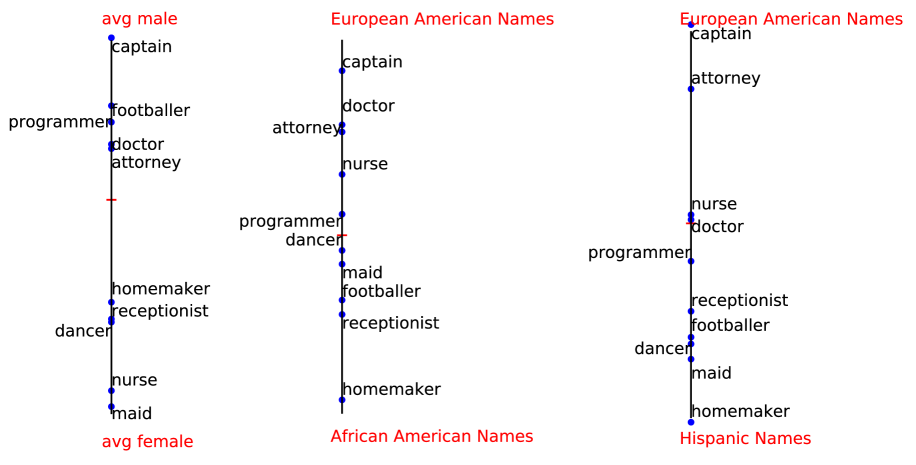
African-American and European-American names. We see a similar trend when we use African-American names and European-American names (Figure 5). We use the African-American names used by Caliskan et al. (2017) [7]. We determine the bias direction by using method in Section 4.1.
We plot in Figure 5 a few occupation words along the axes defined by H-EA and AA-EA bias directions, and compare them with those along the male-female axis. The embedding is different among the groups, and likely still generally more subordinate-biased towards Hispanic and African-American names as it was for female. Although footballer is more Hispanic than European-American, while maid is more neutral in the racial bias setting than the gender setting. We see this pattern repeated across embeddings and datasets (see Supplementary Material A).
When we switch the type of bias, we also end up finding different patterns in the embeddings. In the case of both of these racial directions, there is a the split in not just occupation words but other words that are detected as highly associated with the bias subspace. It shows up foremost among the closest words of the subspace of the bias. Here, we find words like drugs and illegal close to the H-EA direction while, close to the AA-EA direction, we retrieve several slang words used to refer to African-Americans. These word associations with each racial group can be detected by the WEAT tests (lower means less bias) using positive and negative words as demonstrated by Caliskan et al. (2017) [7]. We evaluate using the WEAT test before and after linear projection debiasing in Table 8. For each of these tests, we use half of the names in each category for finding the bias direction and the other half for WEAT testing. This selection is done arbitrarily and the scores are averaged over 3 such selections.
| Before Debiasing | After Debiasing | |
|---|---|---|
| EA-AA | 1.803 | 0.425 |
| EA-H | 1.461 | 0.480 |
| Youth-Aged | 0.915 | 0.704 |
More qualitatively, as a result of the dampening of bias, we see that biased words like other names belonging to these specific demographic groups, slang words, colloquial terms like latinos are removed from the closest 10% words. This is beneficial since the distinguishability of demographic characteristics based on names is what shows up in these different ways like in occupational or financial bias.
Age-associated names.
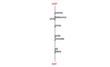
We observed that names can be masked carriers of age too. Using the database for names through time [1] and extracting the most common names from early 1900s as compared to late 1900s and early 2000s, we find a correlation between these names (see Supplementary Material) and age related words. In Figure 6, we see a clear correlation between age and names. Bias in this case does not show up in professions as clearly as in gender but in terms of association with positive and negative words [7]. We again evaluate using a WEAT test in Table 8, the bias before and after debiasing the embedding.
7 DISCUSSION
Different types of bias exist in textual data. Some are easier to detect and evaluate. Some are harder to find suitable and frequent indicators for and thus, to dampen. Gendered word pairs and gendered names are frequent enough in textual data to allow us to successfully measure it in different ways and project the word embeddings away from the subspace occupied by gender. Other types of bias don’t always have a list of word pairs to fall back on to do the same. But using names, as we see here, we can measure and detect the different biases anyway and then project the embedding away from. In this work we also see how a weighted variant of propection removes bias while retaining best the inherent structure of the word embedding.
References
- [1] https://www.ssa.gov/oact/babynames/.
- [2] http://www.babynamewizard.com.
- [3] T Bolukbasi, K W Chang, J Zou, V Saligrama, and A Kalai. Man is to computer programmer as woman is to homemaker? debiasing word embeddings. In ACM Transactions of Information Systems, 2016.
- [4] T Bolukbasi, K W Chang, J Zou, V Saligrama, and A Kalai. Quantifying and reducing bias in word embeddings. 2016.
- [5] Tim Brennan, William Dieterich, and Beate Ehret. Evaluating the predictive validity of the compas risk and needs assessment system. Criminal Justice and Behavior, 36(1):21–40, 2009.
- [6] Kaylee Burns, Lisa Anne Hendricks, Trevor Darrell, and Anna Rohrbach. Women also snowboard: Overcoming bias in captioning models. CoRR, abs/1803.09797, 2018.
- [7] Aylin Caliskan, Joanna J. Bryson, and Arvind Narayanan. Semantics derived automatically from language corpora contain human-like biases. Science, 356(6334):183–186, 2017.
- [8] Christiane Fellbaum. WordNet: An Electronic Lexical Database. Bradford Books, 1998.
- [9] L Finkelstein, E Gabrilovich, Y Matias, E Rivlin, Z Solan, G Wolfman, and etal. Placing search in context : The concept revisited. In ACM Transactions of Information Systems, volume 20, pages 116–131, 2002.
- [10] F Hill, R Reichart, and A Korhonen. Simlex-999 : Evaluating semantic models with (genuine) similarity estimation. In Computational Linguistics, volume 41, pages 665–695, 2015.
- [11] Amir E. Khandani, Adlar J. Kim, and Andrew Lo. Consumer credit-risk models via machine-learning algorithms. Journal of Banking & Finance, 34(11):2767–2787, 2010.
- [12] Omer Levy and Yoav Goldberg. Neural word embedding as implicit matrix factorization. In NIPS, 2013.
- [13] Omer Levy and Yoav Goldberg. Linguistic regularities of sparse and explicit word representations. In CoNLL, 2014.
- [14] Edward Loper and Steven Bird. Nltk: The natural language toolkit. In Proceedings of the ACL-02 Workshop on Effective Tools and Methodologies for Teaching Natural Language Processing and Computational Linguistics - Volume 1, ETMTNLP ’02, pages 63–70, Stroudsburg, PA, USA, 2002. Association for Computational Linguistics.
- [15] Tomas Mikolov, Kai Chen, Greg Corrado, and Jeffrey Dean. Efficient estimation of word representations in vector space. Technical report, arXiv:1301.3781, 2013.
- [16] Tomas Mikolov, Ilya Sutskever, Kai Chen, Greg Corrado, and Jeffrey Dean. Distributed representations of words and phrases and their compositionality. In NIPS, pages 3111–3119, 2013.
- [17] Jeffrey Pennington, Richard Socher, and Christopher D. Manning. Glove: Global vectors for word representation. 2014.
- [18] Jieyu Zhao, Tianlu Wang, Mark Yatskar, Vicente Ordonez, and Kai-Wei Chang. Men also like shopping: Reducing gender bias amplification using corpus-level constraints. CoRR, abs/1707.09457, 2017.
Supplementary material for:
Attenuating Bias in Word Embeddings
Appendix A Bias in different embeddings
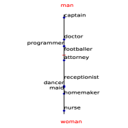
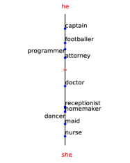
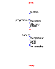
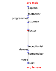
We explore here how gender bias is expressed across different embeddings, datasets and embedding mechanisms. Similar patterns are reflected across all as seen in Figure 7.
For this verification of the permeative nature of bias across datasets and embeddings, we use the GloVe embeddings of a Wikipedia dump (dumps.wikimedia.org/enwiki/latest/enwiki-latest-pages-articles.xml.bz2, B tokens) Common Crawl (B tokens, M vocab) and Twitter (B tokens, M vocab) from https://nlp.stanford.edu/projects/glove/, and the WordToVec embedding of Google News (B tokens, M vocab) from https://code.google.com/archive/p/word2vec/.
(a)
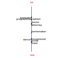
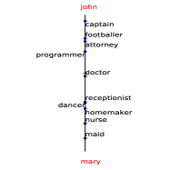
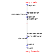
(b) 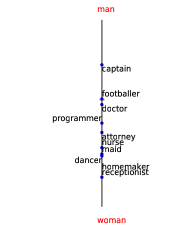
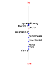
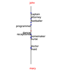
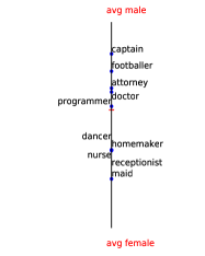
(c) 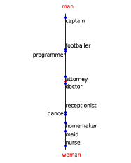
(d) 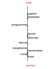
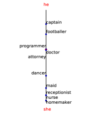
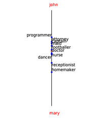
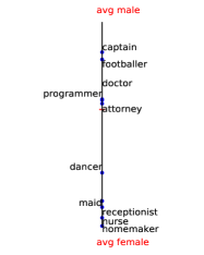
(a) 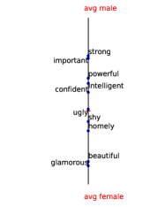 (b)
(b) 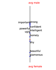 (c)
(c) 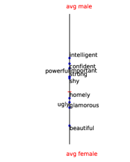 (d)
(d) 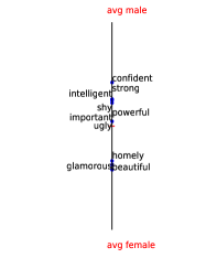
(a) 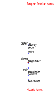 (b)
(b) 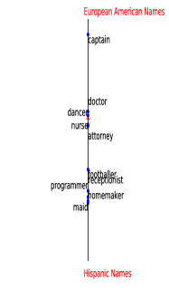
(c) 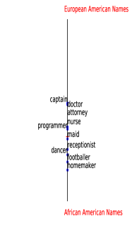 (d)
(d) 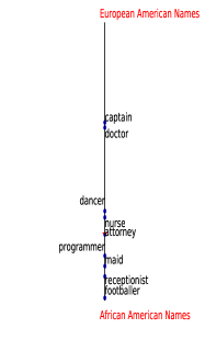
Appendix B WORD EMBEDDING ASSOCIATION TEST
Word Embedding Association Test (WEAT) was defined as an analogue to Implicit Association Test (IAT) by Caliskan et al. [7]. It checks for human like bias associated with words in word embeddings. For example, it found career oriented words (executive, career, etc) more associated with male names and male gendered words (’man’,’boy’ etc) than female names and gendered words and family oriented words (’family’,’home’ etc) more associated with female names and words than male. We list a set of words used for WEAT by Calisan et al. and that we used in our work below.
For two sets of target words X and Y and attribute words A and B, the WEAT test statistic is :
where,
and, is the cosine distance between vector a and b.
This score is normalized by . So, closer to 0 this value is, the less bias or preferential association target word groups have to the attribute word groups.
Here target words are occupation words or career/family oriented words and attributes are male/female words or names.
Career : { executive, management, professional, corporation, salary, office, business, career }
Family : { home, parents, children, family, cousins, marriage, wedding, relatives }
Male names : { john, paul, mike, kevin, steve, greg, jeff, bill }
Female names : { amy, joan, lisa, sarah, diana, kate, ann, donna }
Male words : { male, man, boy, brother, he, him, his, son }
Female words : { female, woman, girl, she, her, hers, daughter }
Appendix C DETECTING THE GENDER DIRECTION
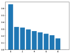
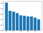
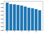
For this, we take a set of gendered word pairs as listed in Table 3. From our default Wikipedia dataset, using the embedded vectors for these word pairs (i.e., (woman - man), (she - he), etc), we create a basis for the subspace , of dimension . We then try to understand the distribution of variance in this subspace. To do so, we project the entire dataset onto this subspace , and take the SVD. The top chart in Figure 10 shows the singular values of the entire data in this subspace . We observe that there is a dominant first singular vector/value which is almost twice the size of the second value. After the this drop, the decay is significantly more gradual. This suggests to use only the top singular vector of as the gender subspace, not or more of these vectors.
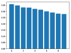
To grasp how much of this variation is from the correlation along the gender direction, and how much is just random variation, we repeat this experiment, again in Figure 10, with different ways of creating the subspace . First in chart (b), we generate vectors, with one word chosen randomly, and one chosen from the gendered set (e.g., chair-woman). Second in chart (c), we generate vectors between two random words from our set of the most frequent words; these are averaged over random iterations due to higher variance in the plots. Finally in chart (d), we generate random unit vectors in . We observe that the pairs with one gendered vector in each pair still exhibits a significant drop in singular values, but not as drastic as with both pairs. The other two approaches have no significant drop since they do not in general contain a gendered word with interesting subspace. All remaining singular values, and their decay appears similar to the non-leading ones from the charts (a) and (b). This further indicates that there is roughly one important gender direction, and any related subspace is not significantly different than a random one in the word-vector embedding.
Now, for any word in vocabulary of the embedding, we can define as the part of along the gender direction.
Based on the experiments shown in Figure 10, it is justified to take the gender direction as the (normalized) first right singular vector, , or the full data set data projected onto the subspace . Then, the component of a word vector along is simply .
Calculating this component when the gender subspace is defined by two or more of the top right singular vectors of can be done similarly.
We should note here that the gender subspace defined here passes through the origin. Centering the data and using PCA to define the gender subspace lets the gender subspace not pass through the origin. We see a comparison in the two methods in Section 5 as uses PCA and we use SVD to define the gender direction.
Appendix D Word Lists
D.1 Word Pairs used for Flipping
actor actress
author authoress
bachelor spinster
boy girl
brave squaw
bridegroom bride
brother sister
conductor conductress
count countess
czar czarina
dad mum
daddy mummy
duke duchess
emperor empress
father mother
father-in-law mother-in-law
fiance fiancee
gentleman lady
giant giantess
god goddess
governor matron
grandfather grandmother
grandson granddaughter
he she
headmaster headmistress
heir heiress
hero heroine
him her
himself herself
host hostess
hunter huntress
husband wife
king queen
lad lass
landlord landlady
lord lady
male female
man woman
manager manageress
manservant maidservant
masseur masseuse
master mistress
mayor mayoress
milkman milkmaid
millionaire millionairess
monitor monitress
monk nun
mr mrs
murderer murderess
nephew niece
papa mama
poet poetess
policeman policewoman
postman postwoman
postmaster postmistress
priest priestess
prince princess
prophet prophetess
proprietor proprietress
shepherd shepherdess
sir madam
son daughter
son-in-law daughter-in-law
step-father step-mother
step-son step-daughter
steward stewardess
sultan sultana
tailor tailoress
uncle aunt
usher usherette
waiter waitress
washerman washerwoman
widower widow
wizard witch
D.2 Occupation Words
detective
ambassador
coach
officer
epidemiologist
rabbi
ballplayer
secretary
actress
manager
scientist
cardiologist
actor
industrialist
welder
biologist
undersecretary
captain
economist
politician
baron
pollster
environmentalist
photographer
mediator
character
housewife
jeweler
physicist
hitman
geologist
painter
employee
stockbroker
footballer
tycoon
dad
patrolman
chancellor
advocate
bureaucrat
strategist
pathologist
psychologist
campaigner
magistrate
judge
illustrator
surgeon
nurse
missionary
stylist
solicitor
scholar
naturalist
artist
mathematician
businesswoman
investigator
curator
soloist
servant
broadcaster
fisherman
landlord
housekeeper
crooner
archaeologist
teenager
councilman
attorney
choreographer
principal
parishioner
therapist
administrator
skipper
aide
chef
gangster
astronomer
educator
lawyer
midfielder
evangelist
novelist
senator
collector
goalkeeper
singer
acquaintance
preacher
trumpeter
colonel
trooper
understudy
paralegal
philosopher
councilor
violinist
priest
cellist
hooker
jurist
commentator
gardener
journalist
warrior
cameraman
wrestler
hairdresser
lawmaker
psychiatrist
clerk
writer
handyman
broker
boss
lieutenant
neurosurgeon
protagonist
sculptor
nanny
teacher
homemaker
cop
planner
laborer
programmer
philanthropist
waiter
barrister
trader
swimmer
adventurer
monk
bookkeeper
radiologist
columnist
banker
neurologist
barber
policeman
assassin
marshal
waitress
artiste
playwright
electrician
student
deputy
researcher
caretaker
ranger
lyricist
entrepreneur
sailor
dancer
composer
president
dean
comic
medic
legislator
salesman
observer
pundit
maid
archbishop
firefighter
vocalist
tutor
proprietor
restaurateur
editor
saint
butler
prosecutor
sergeant
realtor
commissioner
narrator
conductor
historian
citizen
worker
pastor
serviceman
filmmaker
sportswriter
poet
dentist
statesman
minister
dermatologist
technician
nun
instructor
alderman
analyst
chaplain
inventor
lifeguard
bodyguard
bartender
surveyor
consultant
athlete
cartoonist
negotiator
promoter
socialite
architect
mechanic
entertainer
counselor
janitor
firebrand
sportsman
anthropologist
performer
crusader
envoy
trucker
publicist
commander
professor
critic
comedian
receptionist
financier
valedictorian
inspector
steward
confesses
bishop
shopkeeper
ballerina
diplomat
parliamentarian
author
sociologist
photojournalist
guitarist
butcher
mobster
drummer
astronaut
protester
custodian
maestro
pianist
pharmacist
chemist
pediatrician
lecturer
foreman
cleric
musician
cabbie
fireman
farmer
headmaster
soldier
carpenter
substitute
director
cinematographer
warden
marksman
congressman
prisoner
librarian
magician
screenwriter
provost
saxophonist
plumber
correspondent
organist
baker
doctor
constable
treasurer
superintendent
boxer
physician
infielder
businessman
protege
D.3 Names used for Gender Bias Detection
Male : { john, william, george, liam, andrew, michael, louis, tony, scott, jackson }
Female : { mary, victoria, carolina, maria, anne, kelly, marie, anna, sarah, jane }
D.4 Names used for Racial Bias Detection and Dampening
European American : { brad, brendan, geoffrey, greg, brett, matthew, neil, todd, nancy, amanda, emily, rachel }
African American : { darnell, hakim, jermaine, kareem, jamal, leroy, tyrone, rasheed, yvette, malika, latonya, jasmine }
Hispanic : { alejandro, pancho, bernardo, pedro, octavio, rodrigo, ricardo, augusto, carmen, katia, marcella , sofia }
D.5 Names used for Age related Bias Detection and Dampening
Aged : { ruth, william, horace, mary, susie, amy, john, henry, edward, elizabeth }
Youth : { taylor, jamie, daniel, aubrey, alison, miranda, jacob, arthur, aaron, ethan }