Mechanical engineering of photon blockades in a cavity optomechanical system

Abstract

We propose to mechanically control photon blockade (PB) in an optomechanical system with driving oscillators. We show that by tuning the mechanical driving parameters we achieve selective single-photon blockade (1PB) or two-photon blockade (2PB) as well as simultaneous 1PB and 2PB at the same frequency. This mechanical engineering of 1PB and 2PB can be understood from the anharmonic energy levels due to the modulation of the mechanical driving. In contrast to the optomechanical systems without any mechanical driving featuring PB only for specific optical detuning, our results can be useful for achieving novel photon sources with multi-frequency. Our work also opens up new route to mechanically engineer quantum states exhibiting highly nonclassical photon statistics.

I Introduction

Achieving single-photon sources is highly desirable in modern quantum devices, including single-photon transistors F.-Y. Hong2008 , quantum repeaters Y. Han2010 , quantum-optical Josephson interferometer D. Gerace2009 , as well as low-power sensors, qubit gates H.-Z.Wu2010 , and non-classical light switches K. Xia2018 ; S. Zhang2018 ; L. Tang2019 . Over the years, the studies and applications A. Majumdar2013 ; D. E. Chang2007 ; G.W. Lin2015 ; X. Wang2016 ; X.-Y. Lü2015 ; X.-Y. Lü2013 ; I. Carusotto2009 ; M. J. Hartmann2010 of photon blockade (PB) open the possibility of realizing such goal originally proposed in a nonlinear cavity Imamoglu1997 . We note that single-photon blockade (1PB) L. Tian1992 ; Imamoglu1997 , the generation of a single photon in a nonlinear cavity can impede the probability of generating another photon in the cavity, has been experimentally demonstrated in different systems including cavity or circuit cavity quantum electrodynamics systems K. M. Birnbaum2005 ; A. Reinhard2012 ; A. Faraon2008 ; C. Lang2011 ; A. J. Hoffman2011 ; K. Muller2015 and cavity-free devices T. Peyronel2012 . In a recent experiment C. Hamsen2017 , two-photon blockade (2PB) S. S. Shamailov2010 ; C. Hamsen2017 ; A. Miranowicz2013 ; A. Miranowicz2014 ; C. J. Zhu2017 ; G. H. Hovsepyan2014 ; W.-W. Deng2015 has also been demonstrated, opening a route for creating two-photon logic gates. PB requires large nonlinearities which turns out to be highly challenging in practice. However, recently, unconventional PB, even with weak nonlinearities, based on the destructive quantum interferences between different dissipative pathways was theoretically proposed LiewandSavona2010 ; ArkaMajumdar2012 ; W. Zhang2014 ; X. W. Xu2014 ; O. Kyriienko2014 ; Y. H. Zhou2016 ; S. Ferretti2013 ; H. J. Carmichael1985 ; MotoakiBamba2011 ; H. Flayac2017 ; B. Sarma2017 and then experimentally demonstrated H. J. Snijders2018 ; C. Vaneph2018 .

In theoretical studies, PB has also been studied in optical waveguidesD. E. Chang2008 , coupled cavities M. J. Hartmann2006 ; A. D. Greentree2006 ; D. G. Angelakis2007 , circuit-QED Y. X. Liu2014 , gain cavity Y. H. Zhou2018 , spinning resonator RanHuang2018 and optomechanical system (OMS) P. Rabl2011 ; A. Nunnenkamp2011 . We note that in the past decade, cavity optomechanics W. P. Bowen2016 ; M. Aspelmeyer2014 ; T. J. Kippenberg2008 ; M. Metcalfe2014 has significantly extended fundamental studies and practical applications of coherent light-matter interactions, such as optomechanically induced transparency G. S. Agarwal2010 ; S. Weis2010 ; A. H. Safavi-Naeini2011 , ultrasensitive sensing E. Gavartin2012 ; A. G. Krause2012 , storage and transduction of light signals V. Fiore2011 , and the investigation of nonlinear dynamics F. Marquardt2006 . In addition, analogous to PB liaoquad ; H. Wang2015 ; X.W. Xu2013 , phonon blockade H. Seok2017 ; N. Didier2011 ; H. Xie2017 ; H. Xie2018 ; H. Q. Shi2018 ; L.-L. Zheng2019 has also been studied in the OMS, offering a way to study the nonclassicality, entanglement, and dimensionality of the blockaded phonon states.

In this work, we study mechanical engineering of PB in the OMS with a driven oscillator bowen2017 ; 38bowen2016 . This coherent driving of mechanical oscillator has been experimentally realized in the OMS by using Josephson phase qubits OConnell2010 , microwave electrical driven J.Bochmann2013 , and other time-varying weak forces, which provide new tools to control optomechanical devices in applications from precision metrology T.D.Stowe1997 to tunable photonics M.L.Povinelli2005 ; M.Notomi2006 . For example, in recent experiments, mechanical pump was used to break time-reversal symmetry for light propagation Breakingsymmetry2018nature , to observe cascaded optical transparency LFan2015 , and to control spin-phonon coupling A. Barfuss2015 ; I. Yeo2014 . However, previous studies on the role of mechanical pump in an OMS have mainly focused on the classical regimes, e.g., control of transmission rates instead of quantum noises. Here, we study mechanical engineering of PB, a purely quantum effect. We find that, by tuning the strength of the mechanical pump, the multi-frequency PB can be achieved in OMS, which is distinct from previous studies featuring PB only for specific optical detuning. Our results open a new route to study mechanical engineering of purely quantum optomechanical effect, such as mechanical squeezing H. Tan2013 ; A. Kronwald2013 , photon-phonon entanglement C. Joshi2012 ; J. Li2018 .

The remainder of this article is organized as follows. Section II introduces the physical model under our consideration. By theoretically treating the weak-driving term in Hamiltonian as a perturbation, we diagonalize the Hamiltonian and derive the anharmonic energy levels of the system. Then we analytically and numerically calculate the optical correlations of the system and show the mechanical engineering of PB. Finally, Sec. III is a summary and conclusion.

II model and solutions

We consider an OMS schematically illustrated in Fig. 1(a). The cavity is driven by a weak monochromatic laser field with frequency $\omega_{L}$. Meanwhile, a mechanical pump with strength $G$ is applied to excite the mechanical resonator. Moving to the rotating frame with respect to the driving laser field, the Hamiltonian of the system is of the form (hereafter $\hbar=1$)

$$H = H_{s}+H_{d}+H_{p},$$

$$H_{s} = \Delta_{c}a^{\dagger}a+\omega_{m}b^{\dagger}b+g_{0}a^{\dagger}a(b^{\dagger}+b),$$

$$H_{p} = G(\hat{b}^{\dagger}+\hat{b}),$$

$$H_{d} = \Omega(\hat{a}^{\dagger}+\hat{a}).$$ (1)

Here, $a$ ($a^{\dagger}$) and $b$ ($b^{\dagger}$) are, respectively, the annihilation (creation) operators of the optical cavity field and the mechanical mode, with respective resonant frequencies $\omega_{c}$ and $\omega_{m}$. $g_{0}$ represents the single-photon coupling strength between the cavity field and the mechanical resonator. $\Delta_{c}=\omega_{c}-\omega_{L}$ is the detuning between the cavity mode and the driving field. Here, the strong-coupling regime, where the coupling rate $g_{0}$ exceeds the cavity amplitude decay rate $\gamma_{c}$ is required. $H_{s}$ is the Hamiltonian of the OMS without driving term and pumping term. The interaction between the mechanical mode and the pumping field is described as $H_{p}$. The mechanical pump is used to excite phonons in the mechanical mode. The Hamiltonian of the mechanical pump was realized by the cavity electro-optomechanical system consisting of a microtoroidal optomechanical oscillator with an integrated electrical interface that allows a radial force to be applied directly to the mechanical resonator as in Refs. bowen2017 ; 38bowen2016 . $H_{d}$ describes the coupling between the cavity and the weak optical driving laser. The amplitude of the driving field $\Omega$ is related to the input laser power $P_{\text{in}}$ and cavity decay rate $\gamma_{c}$ by $\left|\Omega\right|=\sqrt{P_{\text{in}}\gamma_{c}/\omega_{L}}$.

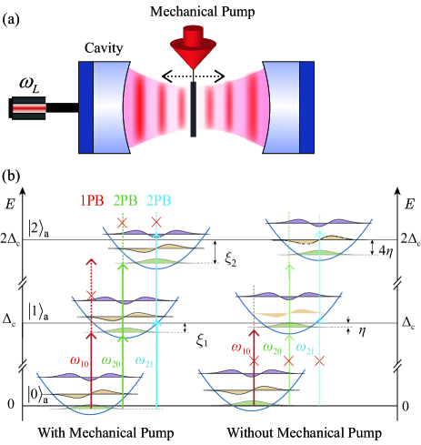
Figure 1: (a) Schematic of the OMS for a Fabry-Perot optical cavity with a moving mirror (mechanical resonator). A mechanical pump with strength $G$ is applied to the mechanical resonator. The mechanical pump was realized by the experimental setup of the cavity electro-optomechanical system consisting of a microtoroidal optomechanical oscillator with an integrated electrical interface that allows a radial force to be applied directly to the mechanical resonator as in Refs. bowen2017 ; 38bowen2016 . (b) Energy-level diagram of the OMS with (the left) and without mechanical pump (the right) for the relevant zero-photon state $\left|0\right\rangle_{a}$, one-photon state $\left|1\right\rangle_{a}$, and two-photon state $\left|2\right\rangle_{a}$.

Here, we show that the Hamiltonian exhibits an anharmonic energy-level configuration, which is crucial to realize 1PB and 2PB. In order to study the eigenenergies of the system, we consider $\left|n\right\rangle_{a}$ and $\left|m\right\rangle_{b}$ ($n,m=0,1,2...$) as the harmonic-osillator number states of the cavity field and the mechanical mode, respectively. We consider a unitary transformation

$$D(n)=\text{exp}[(g_{0}n+G)/\omega_{m}(b-b^{\dagger})],$$ (2)

applied to $H_{s}+H_{p}$, where $n=a^{\dagger}a$. The Hamiltonian $\tilde{H}=D^{\dagger}(H_{s}+H_{p})D$ is generalized with the form

$$\tilde{H}=\Delta_{c}a^{\dagger}a+\omega_{m}b^{\dagger}b-\eta(a^{\dagger}a)^{2}-\delta a^{\dagger}a-\frac{G^{2}}{\omega_{m}}.$$ (3)

Clearly, the Hamiltonian $\tilde{H}$ satisfies

$$\tilde{H}|n\rangle_{a}|m\rangle_{b}=E_{nm}|n\rangle_{a}|m\rangle_{b},$$ (4)

where the eigenvalues are

$$E_{nm}=n\Delta_{c}+m\omega_{m}-n^{2}\eta-n\delta-\frac{G^{2}}{\omega_{m}},$$ (5)

where, $\eta=g^{2}_{0}/\omega_{m}$ and $\delta=2g_{0}G/\omega_{m}$. We multiply the operator $D(n)$ from the two sides of Eq. (4), one can obtain

$$(H_{s}+H_{p})|n\rangle_{a}|\tilde{m}(n)\rangle_{b}=E_{nm}|n\rangle_{a}|\tilde{m}(n)\rangle_{b}.$$ (6)

The $n$-photon displaced number states in Eq. (6) are defined by

$$|\tilde{m}(n)\rangle_{b}=D(n)|m\rangle_{b}.$$ (7)

Especially, $\left|\tilde{m}(0)\right\rangle_{b}=\text{exp}[(G/\omega_{m})(b-b^{\dagger})]\left|m\right\rangle_{b}$. From the Eq. (5), we can know that anharmonic energy levels of the system are obtained based on the nonlinear coupling and the mechanical pump. We note that the energy frequency shift with $n^{2}\eta$ in Eq. (5) is caused by the nonlinear optomechanical interaction, which has been studied in previous literature P. Rabl2011 . Due to the mechanical pump, the energies can be modulated by the terms of $n\delta$ and $G^{2}/\omega_{m}$.

Since the optical driving strength is much smaller than the cavity decay rate, $\Omega\ll\gamma_{c}$, only the lower energy states $|0\rangle_{a}$, $|1\rangle_{a}$, and $|2\rangle_{a}$ of the cavity field are occupied. For convenience, the eigen spectrum of the Hamiltonian $H_{s}+H_{p}$ limited in the zero-, one-, and two-photon cases is shown in Fig. 1(b). The nonlinear resonator exhibits the energy shifts

$$\xi_{n} = \frac{(n^{2}g^{2}_{0}+2ng_{0}G+G^{2})}{\omega_{m}},$$ (8)

in $n$-photon states without phonon sidebands respectively. Without the mechanical pump, i.e., $G=0$, the anharmonicity reduces to $\xi_{n}=n^{2}g^{2}_{0}/\omega_{m}$. When $G\not=0$, this energy shift can be modulated by tuning the strength of the mechanical pump filed, which can be used to realize photon sources with optional frequencies.

In Fig. 1(b), for the input laser frequency $\omega_{L}=\omega_{10}=\omega_{c}-2\eta$, no PB can emerge without mechanical pump. However, for the same driving laser, 1PB can be realized with the mechanical pumping strength $G=g_{0}/2$. Similarly, with the mechanical pump, 2PB corresponding to the transitions $|0\rangle_{a}|\tilde{0}(0)\rangle_{b}\rightarrow|2\rangle_{a}|\tilde{0}(0)\rangle_{b}$ and $|0\rangle_{a}|\tilde{0}(0)\rangle_{b}\rightarrow|2\rangle_{a}|\tilde{2}(2)\rangle_{b}$ can occur for the driving frequency $\omega_{20}$ and $\omega_{21}$, respectively, but can not emerge in the system without the mechanical pump for the same driving frequency. In the OMS without the mechanical pump, 1PB or 2PB occurs at particular optical driving frequency, which fulfills the single-photon or two-photon resonance transition condition. However, by tuning the strength of the mechanical pump, PBs can be realized with optional frequencies. This is a clear signature of mechanical engineering of PBs, which opens up a new route to achieve single-photon or few-photon sources with multi-frequency.

Next, we analytically calculate the second-order and the third-order correlation functions of cavity photons by treating the weak-driving term for Hamiltonian (1) as a perturbation. For the sufficient small $\Omega$, only the lower energy levels of the system are excited. Then the general state of the system in the few-photon subspace can be written as

$$|\psi(t)\rangle = \sum_{n=0}^{n=3}\sum_{m=0}^{\infty}C_{n,m}(t)|n\rangle_{a}|\tilde{m}(n)\rangle_{b},$$ (9)

where coefficients $C_{n,m}$ describe the probability amplitudes of the corresponding states respectively. The single-photon, two-photon, and three-photon displaced number states for the mechanical modes can be obtained from Eq. (7) and read

$$|\tilde{m}(1)\rangle_{b} = \text{exp}[\frac{g_{0}}{\omega_{m}}(b-b^{\dagger})+\frac{G}{\omega_{m}}(b-b^{\dagger})]|m\rangle_{b},$$

$$|\tilde{m}(2)\rangle_{b} = \text{exp}[\frac{2g_{0}}{\omega_{m}}(b-b^{\dagger})+\frac{G}{\omega_{m}}(b-b^{\dagger})]|m\rangle_{b},$$

$$|\tilde{m}(3)\rangle_{b} = \text{exp}[\frac{3g_{0}}{\omega_{m}}(b-b^{\dagger})+\frac{G}{\omega_{m}}(b-b^{\dagger})]|m\rangle_{b}.$$ (10)

Considering the dissipation of the cavity mode (the time in the case of $1/\gamma_{c}\ll t\ll 1/\gamma_{m}$, $\gamma_{m}$ represents the mechanical decay), we phenomenologically add an anti-Hermitian term to Hamiltonian (II) liaoquad . The effective non-Hermitian Hamiltonian takes the form

$$H_{\mathrm{eff}}=H-i\frac{\gamma_{c}}{2}a^{\dagger}a.$$ (11)

In terms of Eqs. (9) and (11), and the Schrödinger equation $id\psi(t)/dt=H_{\mathrm{eff}}\psi(t)$, we obtain the equations of motion for the probability amplitudes

$$\dot{C}_{0,m} = -iE_{0,m}C_{0,m}-i\Omega\sum_{m^{\prime}=0}^{\infty}\,{}_{b}\!\langle\tilde{m}(0)|\tilde{m^{\prime}}(1)\rangle_{b}C_{1,m^{\prime}},$$

$$\dot{C}_{1,m} = -\Gamma_{1}C_{1,m}-i\Omega\sum_{m^{\prime}=0}^{\infty}\,{}_{b}\!\langle\tilde{m}(1)|\tilde{m^{\prime}}(0)\rangle_{b}C_{0,m^{\prime}}$$

$$-i\sqrt{2}\Omega\sum_{m^{\prime}=0}^{\infty}\,{}_{b}\!\langle\tilde{m}(1)|\tilde{m^{\prime}}(2)\rangle_{b}C_{2,m^{\prime}},$$

$$\dot{C}_{2,m} = -\Gamma_{2}C_{2,m}-i\sqrt{2}\Omega\sum_{m^{\prime}=0}^{\infty}\,{}_{b}\!\langle\tilde{m}(2)|\tilde{m^{\prime}}(1)\rangle_{b}C_{1,m^{\prime}}$$

$$-i\sqrt{3}\Omega\sum_{m^{\prime}=0}^{\infty}\,{}_{b}\!\langle\tilde{m}(2)|\tilde{m^{\prime}}(3)\rangle_{b}C_{3,m^{\prime}},$$

$$\dot{C}_{3,m} = -\Gamma_{3}C_{3,m}-i\sqrt{3}\Omega\sum_{m^{\prime}=0}^{\infty}\,{}_{b}\!\langle\tilde{m}(3)|\tilde{m^{\prime}}(2)\rangle_{b}C_{2,m^{\prime}},$$

where $\Gamma_{n}=n\gamma_{c}/2+iE_{n,m}$. These transiton rates can be calculated using the relations ${}_{b}\!\langle\tilde{l}(n^{\prime})|\tilde{k}(n)\rangle_{b}=_{b}\!\langle l|D(n-n^{\prime})|k\rangle_{b}$ and

$${}_{b}\!\langle l|e^{\alpha(b^{\dagger}-b)}|k\rangle_{b}=\begin{cases}\sqrt{\frac{l!}{k!}}e^{-\frac{\alpha^{2}}{2}}(-\alpha)^{k-l}L_{l}^{k-l}(\alpha^{2}),&k\geq l\\ \sqrt{\frac{k!}{l!}}e^{-\frac{\alpha^{2}}{2}}(-\alpha)^{l-k}L_{k}^{l-k}(\alpha^{2}),&l>k\end{cases}$$

where $L_{r}^{s}(x)$ is generalized Laguerre polynomial.

In the weak-driving case, we have the following approximate formulas: $C_{0,m}\sim 1$, $C_{1,m}\sim\Omega/\gamma_{c}$, $C_{2,m}\sim\Omega^{2}/\gamma_{c}^{2}$, $C_{3,m}\sim\Omega^{3}/\gamma_{c}^{3}$. To approximately solve Eq. (II), we neglect the higher-order terms of $\Omega$ in the weak driving regime. Note this approximation has been widely utilized in cavity QED Rebi2002 ; Leach2004 and OMS liaoquad ; Komar2013 for studying the photon statistics. For an initial empty cavity, we have $C_{1,m}(0)=0$, $C_{2,m}(0)=0$, $C_{3,m}(0)=0$; then the long-time solution of Eq. (II) can be approximately obtained as

$$C_{0,m} = C_{0,m}(0)e^{-iE_{0,m}t},$$

$$C_{1,m} = -\Omega\sum_{l=0}^{\infty}\frac{{}_{b}\!\langle\tilde{m}(1)\rangle|\tilde{l}(0)\rangle_{b}C_{0,l}(0)e^{-iE_{0,l}t}}{(E_{1,m}-E_{0,l}-i\frac{\gamma_{c}}{2})},$$

$$C_{2,m} = \sqrt{2}\Omega^{2}\sum_{n,l=0}^{\infty}\frac{{}_{b}\!\langle\tilde{m}(2)|\tilde{n}(1)\rangle_{b}}{(E_{1,n}-E_{0,0}-i\frac{\gamma_{c}}{2})}$$

$$\times\frac{{}_{b}\!\langle\tilde{n}(1)|\tilde{l}(0)\rangle_{b}C_{0,l}(0)e^{-iE_{0,l}t}}{(E_{2,m}-E_{0,l}-i\gamma_{c})},$$

$$C_{3,m} = -\sqrt{6}\Omega^{3}\sum_{m^{\prime},q,l=0}^{\infty}\frac{{}_{b}\!\langle\tilde{m}(3)|\tilde{m^{\prime}}(2)\rangle_{b}\,{}_{b}\!\langle\tilde{m^{\prime}}(2)|\tilde{q}(1)\rangle_{b}}{(E_{1,q}-E_{0,l}-i\frac{\gamma_{c}}{2})}$$

$$\times\frac{{}_{b}\!\langle\tilde{q}(1)|\tilde{l}(0)\rangle_{b}C_{0,l}(0)e^{-iE_{0,l}t}}{(E_{2,m^{\prime}}-E_{0,l}-i\gamma_{c})(E_{3,m}-E_{0,l}-i\frac{3\gamma_{c}}{2})},$$

where $C_{0,m}(0)$ and $C_{0,l}(0)$ are determined by the initial state of the mechanical modes. We assume that the membrane is initially in its ground state $|0\rangle_{b}$, i.e., $C_{0,m}(0)=\delta_{m,0}$. For simplicity, we consider the Taylor expansion of the unitary operators, then the long-time solutions of the system can be obtained from Eq. (II). Accordingly, the probability of zero-photon, one-photon, two-photon and three-photon of the system can be obtained.

The equal-time second-order correlation and the equal-time third-order correlation can be written as $g^{(2)}(0)=2P_{2}/(P_{1}+2P_{2})^{2}$ and $g^{(3)}(0)=6P_{3}/(P_{1}+2P_{2}+3P_{3})^{3}$, i.e.,

$$g^{(2)}(0) = \sum_{m=0}^{\infty}\frac{2|C_{2,m}|^{2}}{(|C_{1,m}|^{2}+2|C_{2,m}|^{2})^{2}},$$ (15)

$$g^{(3)}(0) = \sum_{m=0}^{\infty}\frac{6|C_{3,m}|^{2}}{(|C_{1,m}|^{2}+2|C_{2,m}|^{2}+3|C_{3,m}|^{2})^{3}},$$ (16)

where $P_{1}=\sum_{m=0}^{\infty}\left|C_{1,m}(t)\right|^{2}$, $P_{2}=\sum_{m=0}^{\infty}\left|C_{2,m}(t)\right|^{2}$ and $P_{3}=\sum_{m=0}^{\infty}\left|C_{3,m}(t)\right|^{2}$ are the probabilities for finding a single photon, two photons and three photons in the cavity, respectively.

In the weak-driving case, $P_{1}^{2}\gg P_{2}^{2}$ and $P_{2}^{2}\gg P_{3}^{2}$. Thus, correlation functions are reduced to

$$g^{(2)}(0) \approx \frac{2P_{2}}{P_{1}^{2}},$$ (17)

$$g^{(3)}(0) \approx \frac{6P_{3}}{P_{1}^{3}}.$$ (18)

We now turn to the numerical solution case. In fact, $g^{(2)}(0)=\langle a^{\dagger}a^{\dagger}aa\rangle/\langle a^{\dagger}a\rangle^{2}$ and $g^{(3)}(0)=\langle a^{\dagger}a^{\dagger}a^{\dagger}aaa\rangle/\langle a^{\dagger}a\rangle^{3}$ C. Hamsen2017 . The classical and quantum fluctuations of the environmental degrees of freedom will introduce damping to the cavity field and mechanical oscillator Gardiner2004 ; Walls2008 , as required by the fluctuation-dissipation theorem Kubo1966 . After taking into account both optical and mechanical dissipations, the dynamical evolutoin of the system is described by the master equation

$$\dot{\rho} = i[\rho,H]+\frac{\gamma_{c}}{2}(2a\rho a^{\dagger}-a^{\dagger}a\rho-\rho a^{\dagger}a)$$ (19)

$$+\frac{\gamma_{m}}{2}(\bar{n}_{m}+1)(2b\rho b^{\dagger}-b^{\dagger}b\rho-\rho b^{\dagger}b)$$

$$+\frac{\gamma_{m}}{2}\bar{n}_{m}(2b^{\dagger}\rho b-bb^{\dagger}\rho-\rho bb^{\dagger}),$$

where we assume that the cavity field is connected with a vacuum bath. $\gamma_{m}$ represents the mechanical decay, and $\bar{n}_{m}$ is the average thermal photon number related to the temperature by $\bar{n}_{m}=[\text{exp}(\omega_{m}/k_{B}T_{M})-1]^{-1}$, where $k_{B}$ is the Boltzmann constant, $T_{M}$ is the temperature of the enviroment.

II.1 1PB and 2PB without mechanical pump

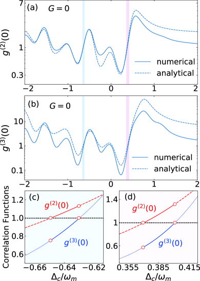
Figure 2: The correlation functions $g^{(2)}(0)$ and $g^{(3)}(0)$ versus $\Delta_{c}/\omega_{m}$ for the OMS without mechanical pump are show in (a),(b) repectively. The solid curves are based the numerical solution of Eq. (19), while the dashed curves are based on the analytical solution of Eq. (II). The case of $g^{(2)}(0)\ll 1$ (i.e., the dip) in (a) indicates 1PB. (c),(d) Correlation functions $g^{(2)}(0)$ and $g^{(3)}(0)$ versus $\Delta_{c}/\omega_{m}$ without mechanical pump. The horizontal black dashed lines show $g^{(n)}(0)=1(n,m=2,3)$ on the basis of Eq. (II.1). The solid lines represent the parameter space satisfying the criterion, the blue dotted and red dashed lines represent the region that does not satisfy the criterion. Figure 3(c) shows 2PB with the two-phonon sidebands, corresponding to $|0\rangle_{a}|\tilde{0}(0)\rangle_{b}\leftrightarrow|2\rangle_{a}|\tilde{0}(2)\rangle_{b}$. Figure 3(d) shows 2PB without phonon sidebands, corresponding to $|0\rangle_{a}|\tilde{0}(0)\rangle_{b}\leftrightarrow|2\rangle_{a}|\tilde{2}(2)\rangle_{b}$. The parameters are taken as $g_{0}/\omega_{m}=0.5$, $\Omega/\omega_{m}=0.01$, $\gamma_{c}/\omega_{m}=0.3$, $\gamma_{m}/\omega_{m}=0.001$ and $\bar{n}_{m}=0$ ($T=0$).

In the OMS without the mechanical pump, i.e., $G=0$, we get the approximate solution of the equal-time second-order and third-order correlation functions

$$g^{(2)}(0) = \frac{4\chi_{1}^{2}+\gamma_{c}^{2}}{4\chi_{2}^{2}+\gamma_{c}^{2}},$$ (20)

$$g^{(3)}(0) = \frac{4(\chi_{1}^{2}+\gamma_{c}^{2})^{2}}{(4\chi_{2}^{2}+\gamma_{c}^{2})(4\chi_{3}^{2}+\gamma_{c}^{2})},$$ (21)

where $\chi_{n}=\Delta_{c}-n\eta$.

Supposing that the driving field is tuned to the single-photon resonantce (SPR) transition frequency, i.e., $\Delta_{c}=g_{0}^{2}/\omega_{m}$, the correlation function becomes

$$g_{\mathrm{SPR}}^{(2)}(0)=\frac{\gamma_{c}^{2}}{4\eta^{2}+\gamma_{c}^{2}}.$$ (22)

In the strong-coupling regime, i.e., $g_{0}>\gamma_{c}$, we have $g_{\text{SPR}}^{(2)}(0)\ll 1$. It means the probability of exciting the single-photon state is higher than that of preparing a two-photon state.

In the case of two-photon resonance (TPR), $\Delta_{c}=2g_{0}^{2}/\omega_{m}$, the equal-time second-order correlation function becomes

$$g_{\mathrm{TPR}}^{(2)}(0)=\frac{4\eta^{2}+\gamma_{c}^{2}}{\gamma_{c}^{2}}.$$ (23)

We have $g^{(2)}(0)>\gg 1$, which indicates that the cavity tends to be in the two-photon state rather than be the single-phonon state. The single-photon or two-phonon transitions can also happen in the $n$-phonon sidebands, as discussed later.

To study 1PB, we calculate the optical correlation function $g^{(2)}(0)$ by using both analytic and numerical method. The condition $g^{(2)}(0)\ll 1$ characterizes 1PB. In order to prove 2PB where the absorption of two photons suppresses the absorption of further photons, it is sufficient to fulfill a necessary criterion, i.e.,

$$g^{(2)}(0) > 1,$$

$$g^{(3)}(0) < 1.$$ (24)

In Figs. 2(a) and 2(b), we plot both the optical correlation functions $g^{(2)}(0)$ and $g^{(3)}(0)$ versus $\Delta_{c}/\omega_{m}$ for $G=0$, of which the analytical and numerical results fit well. In general, $g^{(2)}(0)>1$ stands for a supper-Poisson distribution of the cavity field and $g^{(2)}(0)\gg 1$ corresponds to photon-induced tunneling (PIT). $g^{(2)}(0)<1$ represents the sub-Poisson statistics and $g^{(2)}(0)\ll 1$ corresponds to 1PB signifying nonclassical correlation. The condition $g^{(2)}(0)\rightarrow 0$ means a complete 1PB. As shown in Fig. 2(a), 1PB (i.e., the dip) occurs. The dip corresponds to 1PB and also the SPR case relating to the single-photon process $|0\rangle_{a}|\tilde{0}(0)\rangle_{b}\leftrightarrow|1\rangle_{a}|\tilde{0}(1)\rangle_{b}$. The peak corresponds to PIT and also the two-photon process $|0\rangle_{a}|\tilde{0}(0)\rangle_{b}\leftrightarrow|2\rangle_{a}|\tilde{0}(2)\rangle_{b}$. As a matter of fact, the photon transitions can happen in the $n$-photon sidebands. Figures 2(c) and 2(d) show the correlation functions $g^{(2)}(0)$ and $g^{(3)}(0)$ versus $\Delta_{c}/\omega_{m}$ without mechanical pump. We find 2PB emerges around $\Delta/\omega_{m}=-0.64$ or $\Delta/\omega_{m}=0.385$, corresponding to the transition $|0\rangle_{a}|\tilde{0}(0)\rangle_{b}\leftrightarrow|2\rangle_{a}|\tilde{0}(2)\rangle_{b}$, or two-phonon sideband $|0\rangle_{a}|\tilde{0}(0)\rangle_{b}\leftrightarrow|2\rangle_{a}|\tilde{2}(2)\rangle_{b}$, respectively, which fulfills the correlation given in Eq. (8).

II.2 Mechanical engineering of 1PB and 2PB

In the OMS with the mechanical pump, the equal-time second-order correlation and third-order correlations are modified as

$$g^{(2)}(0) = \frac{4(\chi_{1}-\delta)^{2}+\gamma_{c}^{2}}{4(\chi_{2}-\delta)^{2}+\gamma_{c}^{2}},$$ (25)

$$g^{(3)}(0) = \frac{4[(\chi_{1}-\delta)^{2}+\gamma_{c}^{2}]^{2}}{[4(\chi_{2}-\delta)^{2}+\gamma_{c}^{2}][4(\chi_{3}-\delta)^{2}+\gamma_{c}^{2}]}.$$ (26)

For the SPR case, $\Delta_{c}=g_{0}^{2}+2g_{0}G/\omega_{m}$, the equal-time second-order correlation function is given as:

$$g_{\mathrm{SPR}}^{(2)}(0)=\frac{\gamma_{c}^{2}}{4\eta^{2}+\gamma_{c}^{2}}.$$ (27)

For the TPR case, $\Delta_{c}=(2g_{0}^{2}+2g_{0}G)/\omega_{m}$, the equal-time second-order correlation function is given as:

$$g_{\mathrm{TPR}}^{(2)}(0)=\frac{4\eta^{2}+\gamma_{c}^{2}}{\gamma_{c}^{2}}.$$ (28)

As we can see, the mechanical pump only shifts the optical driving frequency of photon resonances, but doesn’t weak the strength of equal-time correlation functions.

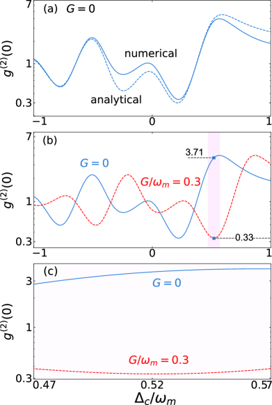
Figure 3: (a) The equal-time second-order correlation function $g^{(2)}(0)$ versus $\Delta_{c}/\omega_{m}$ for the system without mechanical pump, i.e., $G=0$. The dashed curve is the theoretically predicted second-order correlation function and the solid line is from numerical results. (b),(c) numerical equal-time second-order correlation function versus $\Delta_{c}/\omega_{m}$ for $G=0$ and $G/\omega_{m}=0.3$ respectively. The other parameters are the same as Fig. 2.

We now consider the mechanical engineering of $1$PB. In Fig. 3(a), we plot both the analytical and numerical correlation function $g^{(2)}(0)$ versus $\Delta_{c}/\omega_{m}$ for $G/\omega_{m}=0.3$, and the analytical and numerical results are in good agreement. The dashed curve is based on the analytical solutions while the solid curve is based on the numerical results. For the OMS without mechanical pump, $g^{(2)}(0)$ always has a dip at the specific optical detuning $\Delta_{c}/\omega_{m}=0.22\omega_{m}$ or a peak at $\Delta_{c}/\omega_{m}=0.55\omega_{m}$, corresponding to 1PB or PIT, respectively. In contrast, with mechanical pump, by tuning the mechanical strength, a shift for 1PB can be achieved as shown in Fig. 3(b) and  3(c), i.e., $g^{(2)}(0)=3.71$ (no 1PB) for $G=0$, $g^{(2)}(0)=0.33$ (1PB) for $G/\omega_{m}=0.3$. We note that the shift of correlation functions is corresponding to the energy shift given in Eq (8) as mentioned above. The shift can also quantitatively derived by comparing Eq. (20) and Eq. (25). This implies the mechanical engineering of a purely quantum effect, i.e., 1PB. Due to the mechanical strength is tunable, it is also possible to prerpare more feasible single-photon sources with multi-frequencies, which is fundamentally different from the previous studies.

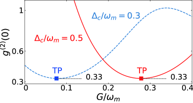
Figure 4: The equal-time second-order correlation function $g^{(2)}(0)$ versus the strength of mechanical pump $G$ for the conditions $\Delta_{c}/\omega_{m}=0.3$ and $\Delta_{c}/\omega_{m}=0.5$, respectively. The other parameters are the same as Fig. 2.

In Fig. 4, we numerically plot correlation function $g^{(2)}(0)$ versus the strength of mechanical pump $G$ under the conditions $\Delta_{c}/\omega_{m}=0.3$ and $\Delta_{c}/\omega_{m}=0.5$ respectively. Clearly for higher mechanical strength, the correlation function gradually changed due to the further shifted energy anharmonicity until reaching the lowest turning point (TP), where 1PB occurs. By deriving the correlation function of Eq. (20), the mechanical strength at TP with the fixed detuning $\Delta_{c}$ then can be given:

$$G=\frac{-3g_{0}^{2}+\sqrt{g_{0}^{4}+\gamma_{c}^{2}}+2\Delta_{c}\omega_{m}}{4g_{0}}.$$ (29)

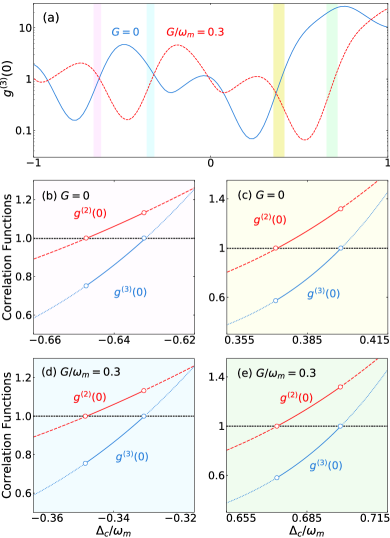
Figure 5: (a) The equal-time third-order correlation function $g^{(3)}(0)$ as a function of $\Delta_{c}/\omega_{m}$ for the strength of $G=0$ (blue solid line) and $G/\omega_{m}=0.5$ (red dashed line) respectively. (b),(c) Correlation functions $g^{(2)}(0)$ (red lines) and $g^{(3)}(0)$ (blue lines) versus $\Delta_{c}/\omega_{m}$ around $\Delta_{c}/\omega_{m}=-0.64$ and $\Delta_{c}/\omega_{m}=0.385$ respectively, with the mechanical strength of $G=0$. (d),(e) Correlation functions $g^{(2)}(0)$ (red lines) and $g^{(3)}(0)$ (blue lines) versus $\Delta_{c}/\omega_{m}$ around $\Delta_{c}/\omega_{m}=-0.34$ and $\Delta_{c}/\omega_{m}=0.685$ respectively, with the mechanical strength of $G/\omega_{m}=0.3$. The horizontal black dashed lines show $g^{(n)}(0)=1(n,m=2,3)$ on the basis of Eq. (II.1). The solid lines in (b-e) represent the parameter space satisfying the criterion, the blue dotted and red dashed lines represent the region that does not satisfy the criterion. The other parameters are the same as Fig. 2.

Owing to the fact that 1PB can be engineered by the mechanical pump, we now consider 2PB. In the following, we show 2PB and the mechanical engineering of 2PB can also be achieved with the mechanical pump.

In Fig. 5(a), we show equal-time third-order correlation function versus the driving detuning $\Delta_{c}/\omega_{m}$ from $G=0$ to $G/\omega_{m}=0.3$, which also be shifted owing to the mechanical pump. Figures 5(b)-(e) show correlation functions $g^{(2)}(0)$ and $g^{(2)}(0)$ versus the driving detuning $\Delta_{c}/\omega_{m}$. The horizontal black dashed lines show $g^{(n)}(0)=1(n,m=2,3)$ on the basis of Eq. (II.1). The solid lines represent the parameters that satisfy the criterion; the blue dotted and red dashed lines represent the region that does not satisfy the criterion. We have found that there are two optical detunings where 2PB occurs. Figures 5(b) and 5(d) indicate 2PB with the two-phonon sidebands, corresponding to $|0\rangle_{a}|\tilde{0}(0)\rangle_{b}\leftrightarrow|2\rangle_{a}|\tilde{0}(2)\rangle_{b}$. Figures 5(c) and  5(e) indicate 2PB without phonon sidebands, corresponding to $|0\rangle_{a}|\tilde{0}(0)\rangle_{b}\leftrightarrow|2\rangle_{a}|\tilde{2}(2)\rangle_{b}$. Obviously, when we change the strength of the mechanical pump from $G=0$ to $G/\omega_{m}=0.3$, 2PB occurs from $\Delta_{c}/\omega_{m}=-0.64$ to $\Delta_{c}/\omega_{m}=-0.34$ with two phonon sidebands, and from $\Delta_{c}/\omega_{m}=0.385$ to $\Delta_{c}/\omega_{m}=0.685$ without phonon sidebands. We note that the difference between two detunings is $\Delta_{c}/\omega_{m}=0.3$ exactly as predicted from fomula (21) and fomula (26).

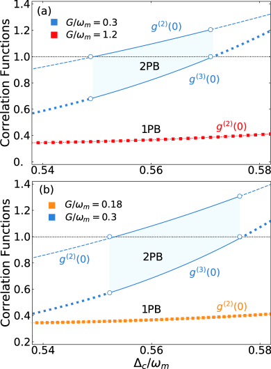
Figure 6: (a),(b) The correlation functions $g^{(2)}(0)$ and $g^{(3)}(0)$ versus $\Delta_{c}/\omega_{m}$. The color codings identify the different strengths of mechanical pump: $G/\omega_{m}=0.3$ (blue lines), $G/\omega_{m}=1.2$ (red line), and $G/\omega_{m}=0.18$ (orange line). The blue backgrounds are regions where 1PB and 2PB can occur at the same driving detuning, with two different strengths of mechanical pump respectively. The other parameters are the same as Fig. 2.

Figure 6 shows the correlation functions $g^{(2)}(0)$ and $g^{(3)}(0)$ versus $\Delta_{c}/\omega_{m}$. The color codings identify the different strengths of mechanical pump: $G/\omega_{m}=0.3$ (blue lines), $G/\omega_{m}=1.2$ (red line), and $G/\omega_{m}=0.18$ (orange line). The blue backgrounds are regions where 1PB and 2PB can occur at the same driving detuning, with two different strengths of mechanical pump respectively. In the presence of mechanical pump, we can achieve both 1PB and 2PB using the same driving laser as indicated by Figs. 6(a) and 6(b). Figure 6(a) corresponds to 2PB without phonon sideband and Fig. 6(b) corresponds to 2PB with two-phonon sidebands. The other parameters are the same as Fig. 2.

III CONCLUSION AND OUTLOOK

In this paper, we analytically and numerically calculate the equal-time second-order and third-order correlation functions of a cavity OMS with a mechanical pump. By properly choosing the strength of mechanical pump, we find the following: (i) selective 1PB or 2PB can be achieved at the adjustable optical detuning. (ii) More interestingly, simultaneous 1PB and 2PB can be achieved at the same driving frequency. This indicates that the mechanical engineering of OMS can provide more flexile control about few-photon emissions. Our work shows that OMS can become another promising platform to achieve such a goal. We note that in very recent experiments, PB or single-photon emission was also observed in driven pendulum-resonator system G. S. Paraoanu2019 or acoustically-driven quantum well system T.-K. Hsiao2019 .

Our work can be further extended to study mechanical engineering of more purely quantum optomechanical effects, such as mechanical squeezing, photon-phonon entanglement. Moreover, due to the mechanical pump’s exceptional operability and convenience nature, the OMS with the mechanical pump is an excellent candidate for exploring new applications from precision metrology to tunable photonics. More interesting than direct-current (scalar) pump, the alternating current mechanical pump in the OMS, including phase effects, will be studied in future work.

Note added. After finishing this work, we became aware of a related work about mechanically controlled single-photon emitter and frequncy comb, by using a membrane-spin hybrid device Plenio2019 .

IV ACKNOWLEDGMENTS

We thank HuiLai Zhang and Tao Liu for useful discussions. This work is supported by NSF of China under Grants No. 11474087 and No. 11774086, and the HuNU Program for Talented Youth.

Appendix A Expansion for a unitary operator $D$ up to the order 1

We consider the limit case of $g_{0}/\omega_{m}\ll 1$. In this case, we can expand the displacement operators $\text{exp}[g_{0}/\omega_{m}(b-b^{\dagger})]$ to $1-g_{0}/\omega_{m}(b-b^{\dagger})$:

$$\left.\left\langle\tilde{m}^{\prime}(1)\right|\tilde{0}(0)\right\rangle_{b} = \delta_{m^{\prime},0}+\frac{g_{0}}{\omega_{m}}\delta_{m^{\prime},1},$$ (30)

$$\left.\left\langle\tilde{m}(1)\right|\tilde{0}\right\rangle_{b}=\delta_{m,0}+\frac{g_{0}}{\omega_{m}}\delta_{m,1},$$ (31)

$$\left.\left\langle\tilde{q}(1)\right|\tilde{0}\right\rangle_{b}=\delta_{q,0}+\frac{g_{0}}{\omega_{m}}\delta_{q,1},$$ (32)

$$\left.\left\langle\tilde{m}(2)\right|\tilde{m}^{\prime}(1)\right\rangle_{b}=\delta_{m,m^{\prime}}+\sqrt{m^{\prime}+1}\frac{g_{0}}{\omega_{m}}\delta_{m,m^{\prime}+1}-\sqrt{m^{\prime}}\frac{g_{0}}{\omega_{m}}\delta_{m,m^{\prime}-1},$$ (33)

$$\left.\left\langle\tilde{m}^{\prime}(2)\right|\tilde{q}(1)\right\rangle_{b}=\delta_{m^{\prime},q}+\sqrt{q+1}\frac{g_{0}}{\omega_{m}}\delta_{m^{\prime},q+1}-\sqrt{q}\frac{g_{0}}{\omega_{m}}\delta_{m^{\prime},q-1},$$ (34)

$$\left.\left\langle\tilde{m}(3)\right|\tilde{m}^{\prime}(2)\right\rangle_{b}=\delta_{m,m^{\prime}}+\sqrt{m^{\prime}+1}\frac{g_{0}}{\omega_{m}}\delta_{m,m^{\prime}+1}-\sqrt{m^{\prime}}\frac{g_{0}}{\omega_{m}}\delta_{m,m^{\prime}-1}.$$ (35)

Appendix B Equal-time third-order correlation function

For the correlations given in Eq. (31), we get the single-photon probability:

$$P_{1} =\sum_{m=0}^{\infty}\left|C_{1}\right|^{2}$$

$$=\sum_{m=0}^{\infty}\left|\frac{-\Omega\left.\left\langle\tilde{m}(1)\right|\tilde{0}\right\rangle_{b}e^{-iE_{0,0}t}}{\Delta_{c}+m\omega_{m}-\frac{g_{0}^{2}+2g_{0}G}{\omega_{m}}-i\frac{\gamma_{c}}{2}}\right|^{2}$$

$$=\sum_{m=0}^{\infty}\frac{\Omega^{2}\left|\left.\left\langle\tilde{m}(1)\right|\tilde{0}\right\rangle_{b}\right|^{2}}{\left(\Delta_{c}+m\omega_{m}-\frac{g_{0}^{2}+2g_{0}G}{\omega_{m}}\right)^{2}+\left(\frac{\gamma_{c}}{2}\right)^{2}}$$

$$=\frac{\Omega^{2}}{\left(\Delta_{c}-\frac{g_{0}^{2}+2g_{0}G}{\omega_{m}}\right)^{2}+\left(\frac{\gamma_{c}}{2}\right)^{2}}+\frac{\Omega^{2}\beta^{2}}{\left(\Delta_{c}+\omega_{m}-\frac{g_{0}^{2}+2g_{0}G}{\omega_{m}}\right)^{2}+\left(\frac{\gamma_{c}}{2}\right)^{2}}.$$ (36)

For three-photon state,

$$C_{3,m}(t) = -\sqrt{6}\Omega^{3}\sum_{m^{\prime},q=0}^{\infty}\frac{\left.\left\langle\tilde{m}(3)\right|\tilde{m}^{\prime}(2)\right\rangle_{b}\left.\left\langle\tilde{m}^{\prime}(2)\right|\tilde{q}(1)\right\rangle_{b}\left.\left\langle\tilde{q}(1)\right|\tilde{0}\right\rangle_{b}e^{-iE_{0,0}t}}{\left(E_{1,q}-E_{0,0}-i\frac{\gamma_{c}}{2}\right)\left(E_{2,m^{\prime}}-E_{0,0}-i\gamma_{c}\right)\left(E_{3,m}-E_{0,0}-i\frac{3\gamma_{c}}{2}\right)},$$ (37)

and three-photon state probability reads

$$P_{3} = \sum_{m=0}^{\infty}\left|C_{3}\right|^{2}$$ (38)

$$\sum_{m=0}^{\infty}\left|\sum_{m^{\prime},q=0}^{\infty}\frac{-\sqrt{6}\Omega^{3}\left.\left\langle\tilde{m}(3)\right|\tilde{m}^{\prime}(2)\right\rangle_{b}\left.\left\langle\tilde{m}^{\prime}(2)\right|\tilde{q}(1)\right\rangle_{b}\left.\left\langle\tilde{q}(1)\right|\tilde{0}\right\rangle_{b}e^{-iE_{0,0}t}}{\left(E_{1,q}-E_{0,0}-i\frac{\gamma_{c}}{2}\right)\left(E_{2,m^{\prime}}-E_{0,0}-i\gamma_{c}\right)\left(E_{3,m}-E_{0,0}-i\frac{3\gamma_{c}}{2}\right)}\right|^{2}$$

$$= 6\Omega^{6}\sum_{m=0}^{\infty}\left|\sum_{m^{\prime}=0}^{\infty}\left.\left\langle\tilde{m}(3)\right|\tilde{m}^{\prime}(2)\right\rangle_{b}U\right|^{2}$$

$$= 6\Omega^{6}\sum_{m=0}^{\infty}\left|V\right|^{2},$$

where

$$U=\sum_{q=0}^{\infty}\frac{\left.\left\langle\tilde{m}^{\prime}(2)\right|\tilde{q}(1)\right\rangle_{b}\left.\left\langle\tilde{q}(1)\right|\tilde{0}\right\rangle_{b}}{\left(E_{1,q}-E_{0,0}-i\frac{\gamma_{c}}{2}\right)\left(E_{2,m^{\prime}}-E_{0,0}-i\gamma_{c}\right)\left(E_{3,m}-E_{0,0}-i\frac{3\gamma_{c}}{2}\right)},$$ (39)

and

$$V=\sum_{m^{\prime}=0}^{\infty}\left.\left\langle\tilde{m}(3)\right|\tilde{m}^{\prime}(2)\right\rangle_{b}U.$$ (40)

Substitutiting Eqs. (33) and (34) into Eq. (39), we can obtain

$$U = \sum_{q=0}^{\infty}\frac{\left.\left\langle\tilde{m}^{\prime}(2)\right|\tilde{q}(1)\right\rangle_{b}\left.\left\langle\tilde{q}(1)\right|\tilde{0}\right\rangle_{b}}{\left(E_{1,q}-E_{0,0}-i\frac{\gamma_{c}}{2}\right)\left(E_{2,m^{\prime}}-E_{0,0}-i\gamma_{c}\right)\left(E_{3,m}-E_{0,0}-i\frac{3\gamma_{c}}{2}\right)}$$ (41)

$$= \sum_{q=0}^{\infty}\frac{\left(\delta_{m^{\prime},q}+\sqrt{q+1}\frac{g_{0}}{\omega_{m}}\delta_{m^{\prime},q+1}-\sqrt{q}\frac{g_{0}}{\omega_{m}}\delta_{m^{\prime},q-1}\right)\left(\delta_{q,0}+\frac{g_{0}}{\omega_{m}}\delta_{q,1}\right)}{\left(E_{1,q}-E_{0,0}-i\frac{\gamma_{c}}{2}\right)\left(E_{2,m^{\prime}}-E_{0,0}-i\gamma_{c}\right)\left(E_{3,m}-E_{0,0}-i\frac{3\gamma_{c}}{2}\right)}$$

$$= \frac{\delta_{m^{\prime},0}+\frac{g_{0}}{\omega_{m}}\delta_{m^{\prime},1}}{\left(E_{1,0}-E_{0,0}-i\frac{\gamma_{c}}{2}\right)\left(E_{2,m^{\prime}}-E_{0,0}-i\gamma_{c}\right)\left(E_{3,m}-E_{0,0}-i\frac{3\gamma_{c}}{2}\right)}$$

$$+\frac{\frac{g_{0}}{\omega_{m}}\left(\delta_{m^{\prime},1}+\sqrt{2}\frac{g_{0}}{\omega_{m}}\delta_{m^{\prime},2}-\frac{g_{0}}{\omega_{m}}\delta_{m^{\prime},0}\right)}{\left(E_{1,1}-E_{0,0}-i\frac{\gamma_{c}}{2}\right)\left(E_{2,m^{\prime}}-E_{0,0}-i\gamma_{c}\right)\left(E_{3,m}-E_{0,0}-i\frac{3\gamma_{c}}{2}\right)}.$$

Substituting Eqs. (35) and (41) into Eq. (40), we can obtain

$$V = \sum_{m^{\prime}=0}^{\infty}\left.\left\langle\tilde{m}(3)\right|\tilde{m}^{\prime}(2)\right\rangle_{b}U$$ (42)

$$= \sum_{m^{\prime}=0}^{\infty}\frac{\left.\left\langle\tilde{m}(3)\right|\tilde{m}^{\prime}(2)\right\rangle_{b}\left(\delta_{m^{\prime},0}+\frac{g_{0}}{\omega_{m}}\delta_{m^{\prime},1}\right)}{\left(E_{1,0}-E_{0,0}-i\frac{\gamma_{c}}{2}\right)\left(E_{2,m^{\prime}}-E_{0,0}-i\gamma_{c}\right)\left(E_{3,m}-E_{0,0}-i\frac{3\gamma_{c}}{2}\right)}$$

$$+\sum_{m^{\prime}=0}^{\infty}\frac{\frac{g_{0}}{\omega_{m}}\left.\left\langle\tilde{m}(3)\right|\tilde{m}^{\prime}(2)\right\rangle_{b}\left(\delta_{m^{\prime},1}+\sqrt{2}\frac{g_{0}}{\omega_{m}}\delta_{m^{\prime},2}-\frac{g_{0}}{\omega_{m}}\delta_{m^{\prime},0}\right)}{\left(E_{1,0}-E_{0,0}-i\frac{\gamma_{c}}{2}\right)\left(E_{2,m^{\prime}}-E_{0,0}-i\gamma_{c}\right)\left(E_{3,m}-E_{0,0}-i\frac{3\gamma_{c}}{2}\right)}$$

$$= \sum_{m^{\prime}=0}^{\infty}\frac{\left(\delta_{m,m^{\prime}}+\sqrt{m^{\prime}+1}\frac{g_{0}}{\omega_{m}}\delta_{m,m^{\prime}+1}-\sqrt{m^{\prime}}\frac{g_{0}}{\omega_{m}}\delta_{m,m^{\prime}-1}\right)\left(\delta_{m^{\prime},0}+\frac{g_{0}}{\omega_{m}}\delta_{m^{\prime},1}\right)}{\left(E_{1,0}-E_{0,0}-i\frac{\gamma_{c}}{2}\right)\left(E_{2,m^{\prime}}-E_{0,0}-i\gamma_{c}\right)\left(E_{3,m}-E_{0,0}-i\frac{3\gamma_{c}}{2}\right)}$$

$$+\sum_{m^{\prime}=0}^{\infty}\frac{\frac{g_{0}}{\omega_{m}}\left(\delta_{m,m^{\prime}}+\sqrt{m^{\prime}+1}\frac{g_{0}}{\omega_{m}}\delta_{m,m^{\prime}+1}-\sqrt{m^{\prime}}\frac{g_{0}}{\omega_{m}}\delta_{m,m^{\prime}-1}\right)\left(\delta_{m^{\prime},1}+\sqrt{2}\frac{g_{0}}{\omega_{m}}\delta_{m^{\prime},2}-\frac{g_{0}}{\omega_{m}}\delta_{m^{\prime},0}\right)}{\left(E_{1,1}-E_{0,0}-i\frac{\gamma_{c}}{2}\right)\left(E_{2,m^{\prime}}-E_{0,0}-i\gamma_{c}\right)\left(E_{3,m}-E_{0,0}-i\frac{3\gamma_{c}}{2}\right)}.$$

When $m^{\prime}=0$, we can obtain

$$V_{0} = \frac{\delta_{m,0}+\frac{g_{0}}{\omega_{m}}\delta_{m,1}}{\left(E_{1,0}-E_{0,0}-i\frac{\gamma_{c}}{2}\right)\left(E_{2,0}-E_{0,0}-i\gamma_{c}\right)\left(E_{3,m}-E_{0,0}-i\frac{3\gamma_{c}}{2}\right)}$$ (43)

$$+\frac{-\frac{g_{0}^{2}}{\omega_{m}^{2}}\left(\delta_{m,0}+\frac{g_{0}}{\omega_{m}}\delta_{m,1}\right)}{\left(E_{1,1}-E_{0,0}-i\frac{\gamma_{c}}{2}\right)\left(E_{2,0}-E_{0,0}-i\gamma_{c}\right)\left(E_{3,m}-E_{0,0}-i\frac{3\gamma_{c}}{2}\right)}.$$

When $m^{\prime}=1$, we can obtain

$$V_{1} = \frac{\frac{g_{0}}{\omega_{m}}\left(\delta_{m,1}+\sqrt{2}\frac{g_{0}}{\omega_{m}}\delta_{m,2}-\frac{g_{0}}{\omega_{m}}\delta_{m,0}\right)}{\left(E_{1,0}-E_{0,0}-i\frac{\gamma_{c}}{2}\right)\left(E_{2,1}-E_{0,0}-i\gamma_{c}\right)\left(E_{3,m}-E_{0,0}-i\frac{3\gamma_{c}}{2}\right)}$$ (44)

$$+\frac{\frac{g_{0}}{\omega_{m}}\left(\delta_{m,1}+\sqrt{2}\frac{g_{0}}{\omega_{m}}\delta_{m,2}-\frac{g_{0}}{\omega_{m}}\delta_{m,0}\right)}{\left(E_{1,1}-E_{0,0}-i\frac{\gamma_{c}}{2}\right)\left(E_{2,1}-E_{0,0}-i\gamma_{c}\right)\left(E_{3,m}-E_{0,0}-i\frac{3\gamma_{c}}{2}\right)}.$$

When $m^{\prime}=2$, we can obtain

$$V_{2} = \frac{\sqrt{2}\frac{g_{0}^{2}}{\omega_{m}^{2}}\left(\delta_{m,2}+\sqrt{3}\frac{g_{0}}{\omega_{m}}\delta_{m,3}-\sqrt{2}\frac{g_{0}}{\omega_{m}}\delta_{m,1}\right)}{\left(E_{1,1}-E_{0,0}-i\frac{\gamma_{c}}{2}\right)\left(E_{2,2}-E_{0,0}-i\gamma_{c}\right)\left(E_{3,m}-E_{0,0}-i\frac{3\gamma_{c}}{2}\right)}.$$ (45)

So we obtain

$$V = V_{0}+V_{1}+V_{2}$$ (46)

$$= \frac{\delta_{m,0}+\frac{g_{0}}{\omega_{m}}\delta_{m,1}}{EHQ_{m}}+\frac{-\frac{g_{0}^{2}}{\omega_{m}^{2}}\left(\delta_{m,0}+\frac{g_{0}}{\omega_{m}}\delta_{m,1}\right)}{FHQ_{m}}$$

$$+\frac{\frac{g_{0}}{\omega_{m}}\left(\delta_{m,1}+\sqrt{2}\frac{g_{0}}{\omega_{m}}\delta_{m,2}-\frac{g_{0}}{\omega_{m}}\delta_{m,0}\right)}{EIQ_{m}}$$

$$+\frac{\frac{g_{0}}{\omega_{m}}\left(\delta_{m,1}+\sqrt{2}\frac{g_{0}}{\omega_{m}}\delta_{m,2}-\frac{g_{0}}{\omega_{m}}\delta_{m,0}\right)}{FIQ_{m}}$$

$$+\frac{\sqrt{2}\frac{g_{0}^{2}}{\omega_{m}^{2}}\left(\delta_{m,2}+\sqrt{3}\frac{g_{0}}{\omega_{m}}\delta_{m,3}-\sqrt{2}\frac{g_{0}}{\omega_{m}}\delta_{m,1}\right)}{FJQ_{m}},$$

where

$$E=E_{1,0}-E_{0,0}-i\frac{\gamma_{c}}{2},$$ (47)

$$F=E_{1,1}-E_{0,0}-i\frac{\gamma_{c}}{2},$$ (48)

$$H=E_{2,0}-E_{0,0}-i\gamma_{c},$$ (49)

$$I=E_{2,1}-E_{0,0}-i\gamma_{c},$$ (50)

$$J=E_{2,2}-E_{0,0}-i\gamma_{c},$$ (51)

$$Q_{m}=E_{3,m}-E_{0,0}-i\frac{3\gamma_{c}}{2}.$$ (52)

When $m=0$, we obtain

$$P_{3,m=0} = 6\Omega^{6}\sum_{m=0}\left|V\right|^{2}$$ (53)

$$= 6\Omega^{6}\sum_{m=0}^{\infty}\left|\frac{1}{EQ_{0}H}-\frac{g_{0}^{2}}{\omega_{m}^{2}FQ_{0}H}-\frac{g_{0}^{2}}{\omega_{m}^{2}EQ_{0}I}-\frac{g_{0}^{2}}{\omega_{m}^{2}FQ_{0}I}\right|^{2}$$

$$= 6\Omega^{6}\left|\frac{FI-\frac{g_{0}^{2}}{\omega_{m}^{2}}EI-\frac{g_{0}^{2}}{\omega_{m}^{2}}HF-\frac{g_{0}^{2}}{\omega_{m}^{2}}HE}{EFQ_{0}HI}\right|^{2}$$

$$\approx 6\Omega^{6}\left|\frac{1}{EQ_{0}H}\right|^{2}.$$

When $m=1$, we obtain

$$P_{3,m=1} = 6\Omega^{6}\sum_{m=1}\left|V\right|^{2}$$ (54)

$$= 6\Omega^{6}\left|\frac{\frac{g_{0}}{\omega_{m}}}{EQ_{1}H}-\frac{\frac{g_{0}^{3}}{\omega_{m}^{3}}}{FQ_{1}H}+\frac{\frac{g_{0}}{\omega_{m}}}{EQ_{1}I}+\frac{\frac{g_{0}}{\omega_{m}}}{FQ_{1}I}-\frac{2\frac{g_{0}^{3}}{\omega_{m}^{3}}}{FQ_{1}J}\right|^{2}$$

$$= 6\Omega^{6}\left|\frac{\frac{g_{0}}{\omega_{m}}F-\frac{g_{0}^{3}}{\omega_{m}^{3}}E}{EFQ_{1}H}+\frac{\frac{g_{0}}{\omega_{m}}F+\frac{g_{0}}{\omega_{m}}E}{EFQ_{1}I}-\frac{2\frac{g_{0}^{3}}{\omega_{m}^{3}}}{FQ_{1}J}\right|^{2}$$

$$\approx 6\Omega^{6}\frac{g_{0}^{2}}{\omega_{m}^{2}}\left|\frac{1}{EQ_{1}H}+\frac{1}{EQ_{1}I}+\frac{1}{FQ_{1}I}\right|^{2}.$$

When $m=2$, we obtain

$$P_{3,m=2} = 6\Omega^{6}\sum_{m=2}\left|V\right|^{2}$$ (55)

$$= 6\Omega^{6}\left|\frac{\sqrt{2}\frac{g_{0}^{2}}{\omega_{m}^{2}}}{EQ_{2}J}+\frac{\sqrt{2}\frac{g_{0}^{2}}{\omega_{m}^{2}}}{FQ_{2}J}+\frac{\sqrt{2}\frac{g_{0}^{2}}{\omega_{m}^{2}}}{FQ_{2}I}\right|^{2}$$

$$= 12\Omega^{6}\frac{g_{0}^{4}}{\omega_{m}^{4}}\left|\frac{1}{EQ_{2}J}+\frac{1}{FQ_{2}J}+\frac{1}{FQ_{2}I}\right|^{2}.$$

When $m=3$, we obtain

$$P_{3,m=3} = 6\Omega^{6}\sum_{m=3}\left|V\right|^{2}$$ (56)

$$= 6\Omega^{6}\left|\frac{\sqrt{6}\frac{g_{0}^{3}}{\omega_{m}^{3}}}{FQ_{3}J}\right|^{2}$$

$$= 36\Omega^{6}\frac{g_{0}^{6}}{\omega_{m}^{6}}\left|\frac{1}{FQ_{3}J}\right|^{2}.$$

In the case of $\frac{g_{0}}{\omega_{m}}\ll 1$ , the terms with high-order can be safely neglected. Consequently the probabilities of finding single, three photons in the cavity are, respectively, rewriten as:

$$P_{1}=\frac{\Omega^{2}}{\left(\Delta_{c}-\frac{g_{0}^{2}+2g_{0}G}{\omega_{m}}\right){}^{2}+\left(\frac{\gamma_{c}}{2}\right){}^{2}},$$ (57)

$$P_{3}=6\Omega^{6}\left|\frac{1}{\left(E_{1,0}-E_{0,0}-i\frac{\gamma_{c}}{2}\right)\left(E_{2,0}-E_{0,0}-i\gamma_{c}\right)\left(E_{3,0}-E_{0,0}-i\frac{3\gamma_{c}}{2}\right)}\right|^{2}.$$ (58)

For the eigenvalus given in Eq. (8) , we obtain

$$E_{0,0}=-\frac{G^{2}}{\omega_{m}},$$ (59)

$$E_{1,0}=\Delta_{c}-\frac{g_{0}^{2}}{\omega_{m}}-\frac{2Gg_{0}}{\omega_{m}}-\frac{G^{2}}{\omega_{m}},$$ (60)

$$E_{2,0}=2\Delta_{c}-\frac{4g_{0}^{2}}{\omega_{m}}-\frac{4Gg_{0}}{\omega_{m}}-\frac{G^{2}}{\omega_{m}},$$ (61)

$$E_{3,0}=3\Delta_{c}-\frac{9g_{0}^{2}}{\omega_{m}}-\frac{6Gg_{0}}{\omega_{m}}-\frac{G^{2}}{\omega_{m}}.$$ (62)

Substituing Eq. (57) and (58) into $g^{(3)}(0)=\frac{6P_{3}}{P_{1}^{3}}$ ,we can obtain the equal-time third-order correlation

$$g^{(3)}(0) =\frac{6P_{3}}{P_{1}^{3}}$$

$$=\frac{36\left[\left(\Delta_{c}-\frac{g_{0}^{2}+2g_{0}G}{\omega_{m}}\right)^{2}+\left(\frac{\gamma_{c}}{2}\right)^{2}\right]}{\left(E_{1,0}-E_{0,0}-i\frac{\gamma_{c}}{2}\right)^{2}\left(E_{2,0}-E_{0,0}-i\gamma_{c}\right)^{2}\left(E_{3,0}-E_{0,0}-i\frac{3\gamma_{c}}{2}\right)^{2}}$$

$$=\frac{36\left[\left(\Delta_{c}-\frac{g_{0}^{2}+2g_{0}G}{\omega_{m}}\right)^{2}+\left(\frac{\gamma_{c}}{2}\right)^{2}\right]^{3}}{\left(\Delta_{c}-\frac{g_{0}^{2}+2Gg_{0}}{\omega_{m}}-i\frac{\gamma_{c}}{2}\right)^{2}\left(2\Delta_{c}-\frac{4g_{0}^{2}+4Gg_{0}}{\omega_{m}}-i\gamma_{c}\right)^{2}\left(3\Delta_{c}-\frac{9g_{0}^{2}+6Gg_{0}}{\omega_{m}}-i\frac{3\gamma_{c}}{2}\right)^{2}}$$

$$=\frac{36\left[\left(\Delta_{c}-\eta-\delta\right)^{2}+\left(\frac{\gamma_{c}}{2}\right)^{2}\right]^{2}}{\left[4\left(\Delta_{c}-2\eta-\delta\right)^{2}+\gamma_{c}^{2}\right]\left[9\left(\Delta_{c}-3\eta-\delta\right)^{2}+\left(\frac{3\gamma_{c}}{2}\right)^{2}\right]}$$

$$=\frac{36\left[4\left(\Delta_{c}-\eta-\delta\right)^{2}+4\left(\frac{\gamma_{c}}{2}\right)^{2}\right]^{2}}{4\left[4\left(\Delta_{c}-2\eta-\delta\right)^{2}+\gamma_{c}^{2}\right]\left[36\left(\Delta_{c}-3\eta-\delta\right)^{2}+4\left(\frac{3\gamma_{c}}{2}\right)^{2}\right]}$$

$$=\frac{\left[4\left(\Delta_{c}-\eta-\delta\right)^{2}+\left(\gamma_{c}\right)^{2}\right]^{2}}{\left[4\left(\Delta_{c}-2\eta-\delta\right)^{2}+\gamma_{c}^{2}\right]\left[4\left(\Delta_{c}-3\eta-\delta\right)^{2}+\left(\gamma_{c}\right)^{2}\right]}.$$ (63)

References

• (1) F.-Y. Hong and S.-J. Xiong, Single-photon transistor using microtoroidal resonators, Phys. Rev. A 78, 013812 (2008).
• (2) Y. Han, B. He, K. Heshami, C.-Z. Li, and C. Simon, Quantum repeaters based on Rydberg-blockade-coupled atomic ensembles, Phys. Rev. A 81, 052311 (2010).
• (3) D. Gerace, H. E. Türeci, A. Imamoǧlu, V. Giovannetti, and R. Fazio, The quantum-optical Josephson interferometer, Nat. Phys. 5, 281 (2009).
• (4) H.-Z.Wu, Z.-B.Yang, and S.-B. Zheng, Implementation of a multiqubit quantum phase gate in a neutral atomic ensemble via the asymmetric Rydberg blockade, Phys. Rev. A 82, 034307 (2010).
• (5) K. Xia, F. Nori, and M. Xiao, Cavity-Free Optical Isolators and Circulators Using a Chiral Cross-Kerr Nonlinearity, Phys. Rev. Lett. 121, 203602 (2018).
• (6) S. Zhang, Y. Hu, G. Lin, Y. Niu, K. Xia, J. Gong, and S. Gong, Thermal-motion-induced non-reciprocal quantum optical system, Nat. Photonics 12, 744 (2018).
• (7) L. Tang, J. Tang, W. Zhang, G. Lu, H. Zhang, Y. Zhang, K. Xia, and M. Xiao, arXiv:1811.02957.
• (8) A. Majumdar and D. Gerace, Single-photon blockade in doubly resonant nanocavities with second-order nonlinearity, Phys. Rev. B 87, 235319 (2013)
• (9) D. E. Chang, A. S. Sorensen, E. A. Demler, and M. D. Lukin, A single-photon transistor using nanoscale surface plasmons, Nat. Phys. 3, 807 (2007).
• (10) G. W. Lin, Y. H. Qi, X. M. Lin, Y. P. Niu, and S. Q. Gong, Strong photon blockade with intracavity electromagnetically induced transparency in a blockaded Rydberg ensemble, Phys. Rev. A 92, 043842 (2015).
• (11) X.-Y. Lü, Y. Wu, J. R. Johansson, H. Jing, J. Zhang, and F. Nori, Squeezed Optomechanics with Phase-Matched Amplification and Dissipation, Phys. Rev. Lett. 114, 093602 (2015).
• (12) X.-Y. Lü, W.-M. Zhang, S. Ashhab, Y. Wu, and F. Nori, Quantum-criticality-induced strong Kerr nonlinearities in optomechanical systems, Sci. Rep. 3, 2943 (2013).
• (13) X. Wang, A. Miranowicz, H.-R. Li, and F. Nori, Method for observing robust and tunable phonon blockade in a nanomechanical resonator coupled to a charge qubit, Phys. Rev. A 93, 063861 (2016).
• (14) I. Carusotto, D. Gerace, H. E. Tureci, S. De Liberato, C. Ciuti, and A. Imamoǧlu, Fermionized Photons in an Array of Driven Dissipative Nonlinear Cavities, Phys. Rev. Lett. 103, 033601 (2009).
• (15) M. J. Hartmann, Polariton Crystallization in Driven Arrays of Lossy Nonlinear Resonators, Phys. Rev. Lett. 104, 113601 (2010).
• (16) A. Imamoǧlu, H. Schmidt, G. Woods, and M. Deutsch, Strongly Interacting Photons in a Nonlinear Cavity, Phys. Rev. Lett. 79, 1467 (1997).
• (17) L. Tian and H. J. Carmichael, Quantum trajectory simulations of two-state behavior in an optical cavity containing one atom, Phys. Rev. A 46, R6801 (1992).
• (18) K. M. Birnbaum, A. Boca, R. Miller, A. D. Boozer, T. E. Northup, and H. J. Kimble, Photon blockade in an optical cavity with one trapped atom, Nature (London) 436, 87 (2005).
• (19) A. Reinhard, T. Volz, M. Winger, A. Badolato, K. J. Hennessy, E. L. Hu, and A. Imamoǧlu, Strongly correlated photons on a chip, Nat. Photonics 6, 93 (2012).
• (20) C. Lang, D. Bozyigit, C. Eichler, L. Steffen, J. M. Fink, A. A. Abdumalikov, M. Baur, S. Filipp, M. P. da Silva, A. Blais, and A. Wallraff, Observation of Resonant Photon Blockade at Microwave Frequencies Using Correlation Function Measurements, Phys. Rev. Lett. 106, 243601 (2011).
• (21) A. Faraon, I. Fushman, D. Englund, N. Stoltz, P. Petroff, and J. Vučković, Coherent generation of non-classical light on a chip via photon-induced tunnelling and blockade, Nat. Phys. 4, 859 (2008).
• (22) A. J. Hoffman, S. J. Srinivasan, S. Schmidt, L. Spietz, J. Aumentado, H. E. Tureci, and A. A. Houck, Dispersive Photon Blockade in a Superconducting Circuit, Phys. Rev. Lett. 107, 053602 (2011).
• (23) K. Müller, A. Rundquist, K. A. Fischer, T. Sarmiento, K. G. Lagoudakis, Y. A. Kelaita, C. S. Muñoz, E. del Valle, F. P. Laussy, and J. Vučković, Coherent Generation of Nonclassical Light on Chip via Detuned Photon Blockade, Phys. Rev. Lett. 114, 233601 (2015).
• (24) T. Peyronel, O. Firstenberg, Q.-Y. Liang, S. Hofferberth, A. V. Gorshkov, T. Pohl, M. D. Lukin, and V. Vuletić, Quantum nonlinear optics with single photons enabled by strongly interacting atoms, Nature (London) 488, 57 (2012).
• (25) C. Hamsen, K. N. Tolazzi, T. Wilk, and G. Rempe, Two-Photon Blockade in an Atom-Driven Cavity QED System, Phys. Rev. Lett. 118, 133604 (2017).
• (26) G. H. Hovsepyan, A. R. Shahinyan, and G. Y. Kryuchkyan, Multiphoton blockades in pulsed regimes beyond stationary limits, Phys. Rev. A 90, 013839 (2014).
• (27) A. Miranowicz, J. Bajer, M. Paprzycka, Y.-x. Liu, A. M. Zagoskin, and F. Nori, State-dependent photon blockade via quantum-reservoir engineering, Phys. Rev. A 90, 033831 (2014).
• (28) S. S. Shamailov, A. S. Parkins, M. J. Collett, and H. J. Carmichael, Multi-photon blockade and dressing of the dressed states, Opt. Commun. 283, 766 (2010).
• (29) A. Miranowicz, M. Paprzycka, Y.-x. Liu, J. Bajer, and F. Nori, Two-photon and three-photon blockades in driven nonlinear systems, Phys. Rev. A 87, 023809 (2013).
• (30) C. J. Zhu, Y. P. Yang, and G. S. Agarwal, Collective multiphoton blockade in cavity quantum electrodynamics, Phys. Rev. A 95, 063842 (2017).
• (31) W.-W. Deng, G.-X. Li, and H. Qin, Enhancement of the two-photon blockade in a strong-coupling qubit-cavity system, Phys. Rev. A 91, 043831 (2015).
• (32) T. C. H. Liew and V. Savona, Single Photons from Coupled Quantum Modes, Phys. Rev. Lett. 104, 183601 (2010).
• (33) A. Majumdar, M. Bajcsy, A. Rundquist, and J. Vučkovič, Loss-Enabled Sub-Poissonian Light Generation in a Bimodal Nanocavity, Phys. Rev. Lett. 108, 183601 (2012).
• (34) W. Zhang, Z. Y. Yu, Y. M. Liu, and Y. W. Peng, Optimal photon antibunching in a quantum-dot-bimodal-cavity system, Phys. Rev. A 89, 043832 (2014).
• (35) X. W. Xu and Y. Li, Strong photon antibunching of symmetric and antisymmetric modes in weakly nonlinear photonic molecules, Phys. Rev. A 90, 033809 (2014).
• (36) O. Kyriienko, I. A. Shelykh, and T. C. H. Liew, Tunable singlephoton emission from dipolaritons, Phys. Rev. A 90, 033807 (2014).
• (37) Y. H. Zhou, H. Z. Shen, X. Q. Shao, and X. X. Yi, Strong photon antibunching with weak second-order nonlinearity under dissipation and coherent driving, Opt. Express 24, 17332 (2016).
• (38) S. Ferretti, V. Savona, and D. Gerace, Optimal antibunching in passive photonic devices based on coupled nonlinear resonators, New J. Phys. 15, 025012 (2013).
• (39) B. Sarma and A. K. Sarma, Quantum-interference-assisted photon blockade in a cavity via parametric interactions, Phys. Rev. A 96, 053827 (2017).
• (40) H. J. Carmichael, Photon Antibunching and Squeezing for a Single Atom in a Resonant Cavity, Phys. Rev. Lett. 55, 2790 (1985).
• (41) M. Bamba, A. Imamoǧlu, I. Carusotto, and C. Ciuti, Origin of strong photon antibunching in weakly nonlinear photonic molecules, Phys. Rev. A 83, 021802 (2011).
• (42) H. Flayac and V. Savona, Unconventional photon blockade, Phys. Rev. A 96, 053810 (2017).
• (43) C. Vaneph, A. Morvan, G. Aiello, M. Féchant, M. Aprili, J. Gabelli, and J. Estève, Observation of the Unconventional Photon Blockade in the Microwave Domain, Phys. Rev. Lett. 121, 043602 (2018).
• (44) H. J. Snijders, J. A. Frey, J. Norman, H. Flayac, V. Savona, A. C. Gossard, J. E. Bowers, M. P. van Exter, D. Bouwmeester, and W. Löffler, Observation of the Unconventional Photon Blockade, Phys. Rev. Lett. 121, 043601 (2018).
• (45) D. E. Chang, V. Gritsev, G.Morigi, V. Vuletić, M. D. Lukin, and E. A. Demler, Crystallization of strongly interacting photons in a nonlinear optical fibre, Nat. Phys. 4, 884 (2008).
• (46) M. J. Hartmann, F. G. S. L. Brandao, and M. B. Plenio, Strongly interacting polaritons in coupled arrays of cavities, Nat. Phys. 2, 849 (2006).
• (47) A. D. Greentree, C. Tahan, J. H. Cole, and L. C. L. Hollenberg, Quantum phase transitions of light, Nat. Phys. 2, 856 (2006).
• (48) D. G. Angelakis, M. F. Santos, and S. Bose, Photon-blockade-induced Mott transitions and XY spin models in coupled cavity arrays, Phys. Rev. A 76, 031805 (2007).
• (49) Y.-x. Liu, X. W. Xu, A.Miranowicz, and F. Nori, From blockade to transparency: Controllable photon transmission through a circuit-QED system, Phys. Rev. A 89, 043818 (2014).
• (50) Y. H. Zhou, H. Z. Shen, X. Y. Zhang, and X. X. Yi, Zero eigenvalues of a photon blockade induced by a non-Hermitian Hamiltonian with a gain cavity, Phys. Rev. A 97, 043819 (2018).
• (51) R. Huang, A. Miranowicz, , F. Nori, and H. Jing, Nonreciprocal Photon Blockade, Phys. Rev. Lett. 121, 153601 (2018).
• (52) P. Rabl, Photon Blockade Effect in Optomechanical Systems, Phys. Rev. Lett. 107, 063601 (2011).
• (53) A. Nunnenkamp, K. Børkje, and S. M. Girvin, Single-Photon Optomechanics, Phys. Rev. Lett. 107, 063602 (2011).
• (54) W. P. Bowen, G. J. Milburn, Quantum Optomechanics, (CRC Press, 2016).
• (55) M. Aspelmeyer, T. J. Kippenberg, and F. Marquardt, Cavity optomechanics, Rev. Mod. Phys. 86, 1391 (2014).
• (56) M. Metcalfe, Applications of cavity optomechanics, Appl. Phys. Rev. 1, 031105 (2014).
• (57) T. J. Kippenberg and K. J. Vahala, Cavity optomechanics: back-action at the mesoscal, Science 321, 1172 (2008).
• (58) G. S. Agarwal and S. M. Huang, Electromagnetically induced transparency in mechanical effects of light, Phys. Rev. A 81, 041803 (2010).
• (59) S. Weis, R. Rivière , S. Deléglise, E. Gavartin, O. Arcizet, A. Schliesser, and T. J. Kippenberg, Optomechanically induced transparency, Science 330, 1520 (2010).
• (60) A. H. Safavi-Naeini, T. P. M. Alegre, J. Chan, M. Eichenfield, M. Winger, Q. Lin, J. T. Hill, D. E. Chang, and O. Painter, Electromagnetically induced transparency and slow light with optomechanics, Nature (London) 472, 69 (2011).
• (61) E. Gavartin, P. Verlot, and T. J. Kippenberg, A hybrid on-chip optomechanical transducer for ultrasensitive force measurements, Nat. Nanotechnol. 7, 509 (2012).
• (62) A. G. Krause, M. Winger, T. D. Blasius, Q. Lin, and O. Painter, A high-resolution microchip optomechanical accelerometer, Nat. Photonics 6, 768 (2012).
• (63) V. Fiore, Y. Yang, M. C. Kuzyk, R. Barbour, L. Tian, and H. Wang, Storing Optical Information as a Mechanical Excitation in a Silica Optomechanical Resonator, Phys. Rev. Lett. 107, 133601 (2011).
• (64) F. Marquardt, J. G. E. Harris, and S. M. Girvin, Dynamical Multistability Induced by Radiation Pressure in High-Finesse Micromechanical Optical Cavities, Phys. Rev. Lett. 96, 103901 (2006).
• (65) J.-Q. Liao and F. Nori, Photon blockade in quadratically coupled optomechanical systems, Phys. Rev. A 88, 023853 (2013).
• (66) H. Wang, X. Gu, Y.-x. Liu, A. Miranowicz, and F. Nori, Tunable photon blockade in a hybrid system consisting of an optomechanical device coupled to a two-level system, Phys. Rev. A 92, 033806 (2015).
• (67) X. W. Xu and Y. J. Li, Antibunching photons in a cavity coupled to an optomechanical system, J. Phys. B 46, 035502 (2013).
• (68) H. Seok and E. M. Wright, Antibunching in an optomechanical oscillator, Phys. Rev. A 95, 053844 (2017).
• (69) H. Xie, C. G. Liao, X. Shang, M. Y. Ye, and X. M. Lin, Phonon blockade in a quadratically coupled optomechanical system, Phys. Rev. A 96, 013861 (2017).
• (70) N. Didier, S. Pugnetti, Y. M. Blanter, and R. Fazio, Detecting phonon blockade with photons, Phys. Rev. B 84, 054503 (2011).
• (71) H. Xie, C. G. Liao, X. Shang, Z. H. Chen, and X. M. Lin, Optically induced phonon blockade in an optomechanical system with second-order nonlinearity, Phys. Rev. A 98, 023819 (2018).
• (72) H. Q. Shi, X. T. Zhou, X. W. Xu, and N. H. Liu, Tunable phonon blockade in quadratically coupled optomechanical systems, Sci. Rep. 8, 2212 (2018).
• (73) L.-L. Zheng, T.-S. Yin, Qian Bin, X.-Y. Lü and Ying Wu, Single-photon-induced phonon blockade in a hybrid spin-optomechanical system, Phys. Rev. A 99, 013804 (2019).
• (74) C. Bekker, R. Kalra, C. Baker, and W. P. Bowen, Injection locking of an electro-optomechanical device, Optica 4, 1196 (2017).
• (75) C. G. Baker, C. Bekker, D. L. Mcauslan, E. Sheridan, and W. P. Bowen, High bandwidth on-chip capacitive tuning of microtoroid resonators, Opt. Express 24, 20400 (2016).
• (76) A. D. ÓConnell, M. Hofheinz, M. Ansmann, R. C. Bialczak, M. Lenander, E. Lucero, M. Neeley, D. Sank, H. Wang, M. Weides, J. Wenner, J. M. Martinis, and A. N. Cleland, Quantum ground state and single-phonon control of a mechanical resonator, Nature (London) 464, 697 (2010).
• (77) J. Bochmann, A. Vainsencher, D. D. Awschalom, and A. N. Cleland, Nanomechanical coupling between microwave and optical photons, Nat. Phys. 9, 712 (2013).
• (78) T. D. Stowe, K. Yasumura, T. W. Kenny, D. Botkin, K. Wago, and D. Rugar, Attonewton force detection using ultrathin silicon cantilevers, Appl. Phys. Lett. 71, 288 (1997).
• (79) M. L. Povinelli, M. Loncar, M. Ibanescu, E. J. Smythe, S. G. Johnson, F. Capasso, and J. D. Joannopoulos, Evanescent-wave bonding between optical waveguides, Opt. Lett. 30, 3042 (2005).
• (80) M. Notomi, H. Taniyama, S. Mitsugi, and E. Kuramochi, Optomechanical Wavelength and Energy Conversion in High-Double-Layer Cavities of Photonic Crystal Slabs, Phys. Rev. Lett. 97, 023903 (2006).
• (81) D. B. Sohn, S. Kim and G. Bahl, Time-reversal symmetry breaking with acoustic pumping of nanophotonic circuits, Nat. Photonics 12, 91 (2018).
• (82) L. Fan, K. Y. Fong, M. Poot, and H. X. Tang, Cascaded optical transparency in multimode-cavity optomechanical systems, Nat. Commun. 6, 5850 (2015).
• (83) A. Barfuss, J. Teissier, E. Neu, A. Nunnenkamp and P. Maletinsky, Strong mechanical driving of a single electron spin, Nat. Phys. 11, 820 (2015).
• (84) I. Yeo, P. L. de Assis, A. Gloppe, E. Dupont-Ferrier, P. Verlot, N. S. Malik, E. Dupuy, J. Claudon, J. M. Gerard, A. Auffeves, G. Nogues, S. Seidelin, J. P. Poizat, O. Arcizet, and M. Richard, Strain-mediated coupling in a quantum dot-mechanical oscillator hybrid system, Nat. Nanotechnol. 9, 106 (2014).
• (85) H. Tan, G. Li, and P. Meystre, Dissipation-driven two-mode mechanical squeezed states in optomechanical systems, Phys. Rev. A 87, 033829 (2013).
• (86) A. Kronwald, F. Marquardt, and A. A. Clerk, Arbitrarily large steady-state bosonic squeezing via dissipation, Phys. Rev. A 88, 063833 (2013).
• (87) C. Joshi, J. Larson, M. Jonson, E. Andersson, and P. Öhberg, Phys. Rev. A 85, 033805 (2012)
• (88) J. Li, S.-Y. Zhu, and G. S. Agarwal, Magnon-Photon-Phonon Entanglement in Cavity Magnomechanics, arXiv:1807.07158.
• (89) S. Rebić, A. S. Parkins, and S. M. Tan, Polariton analysis of a four-level atom strongly coupled to a cavity mode, Phys. Rev. A 65, 043806 (2002).
• (90) J. Leach and P. R. Rice, Cavity QED with Quantized Center of Mass Motion, Phys. Rev. Lett. 93, 103601 (2004).
• (91) P. Komar, S. D. Bennett, K. Stannigel, S. J. M. Habraken, P. Rabl, P. Zoller, and M. D. Lukin, Single-photon nonlinearities in two-mode optomechanics, Phys. Rev. A 87, 013839 (2013).
• (92) C. W. Gardiner and P. Zoller, Quantum Noise, (Springer, Berlin, 2004).
• (93) D. Walls and G. J.Milburn, Quantum Optics, (Springer, Berlin, 2008).
• (94) R. Kubo, The fluctuation-dissipation theorem, Rep. Prog. Phys. 29, 255 (1966).
• (95) I. Pietikäi̇nen, J. Tuorila, D. S. Golubev, and G. S. Paraoanu, Quantum-to-classical transition in the driven-dissipative Josephson pendulum coupled to a resonator, arXiv:1901.05655.
• (96) T.-K. Hsiao, A. Rubino, Y. Chung, S.-K. Son, H. Hou, J. Pedrós, A. Nasir, G. Éthier-Majcher, M. J. Stanley, R. T. Phillips, T. A. Mitchell, J. P. Griffiths, I. Farrer, D. A. Ritchie, and C. J. B. Ford, Single-photon Emission from an Acoustically-driven Lateral Light-emitting Diode, arXiv:1901.03464.
• (97) M. Abdi and M. B. Plenio, Quantum Effects in a Mechanically Modulated Single-Photon Emitter, Phys. Rev. Lett. 122, 023602 (2019).