Pegasus: The second connectivity graph for large-scale quantum annealing hardware
Abstract
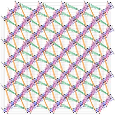
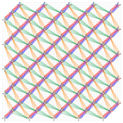
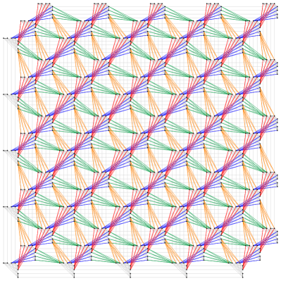
Pegasus is a graph which offers substantially increased connectivity between the qubits of quantum annealing hardware compared to the graph Chimera. It is the first fundamental change in the connectivity graph of quantum annealers built by D-Wave since Chimera was introduced in 2009 and then used in 2011 for D-Wave’s first commercial quantum annealer. In this article we describe an algorithm which defines the connectivity of Pegasus and we provide what we believe to be the best way to graphically visualize Pegasus in order to see which qubits couple to each other. As supplemental material, we provide a wide variety of different visualizations of Pegasus which expose different properties of the graph in different ways. We provide an open source code for generating the many depictions of Pegasus that we show.
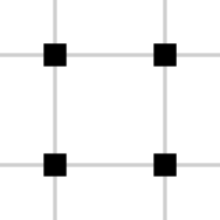
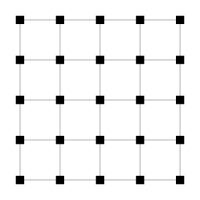
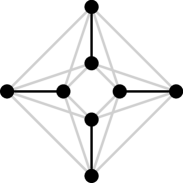
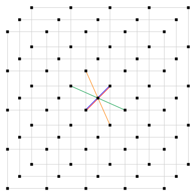
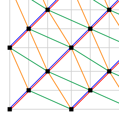
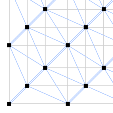
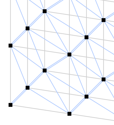
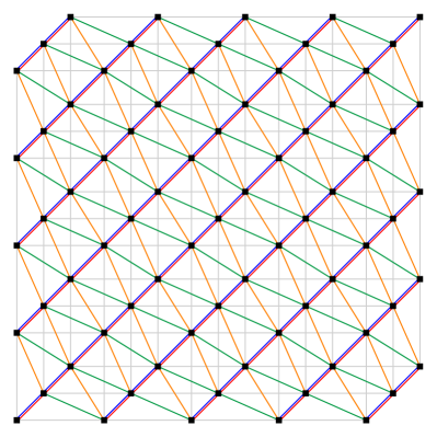
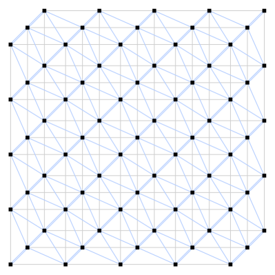
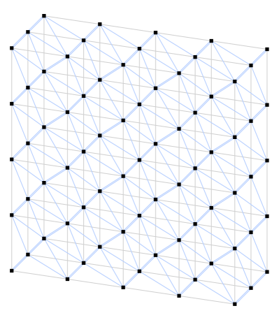
The 128 qubits of the first commercial quantum annealer (D-Wave One, released in 2011) were connected by a graph called Chimera (first defined publicly in 2009 (Neven et al., 2009)), which is rather easy to describe: A 2D array of graphs, with one ‘side’ of each being connected to the same corresponding side on the cells directly above and below it, and the other side being connected to the same corresponding side on the cells to the right and left of it (see Figure 1). The qubits can couple to up to 6 other qubits, since each qubit couples to 4 qubits within its unit cell, and to 2 qubits in the cells above and below it, or to the left and right of it. All commercial quantum annealers built to date follow this graph connectivity, with just larger and larger numbers of cells (see Table 1).
| Array of cells | Total # of qubits | |
|---|---|---|
| D-Wave One | 128 | |
| D-Wave Two | 512 | |
| D-Wave 2X | 1152 | |
| D-Wave 2000Q | 2048 |
In 2018, D-Wave announced the construction of a (not yet commercial) quantum annealer with a greater connectivity than Chimera offers, and a program (NetworkX) which allows users to generate certain Pegasus graphs. However, no explicit description of the graph connectivity in Pegasus has been published yet, so we have had to apply the process of reverse engineering to determine it, and the following section describes the algorithm we have established for generating Pegasus.
I Algorithm for generating Pegasus
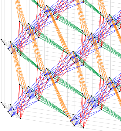
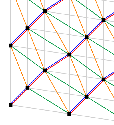
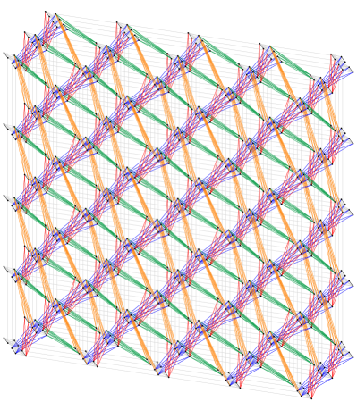
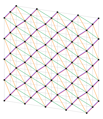
are part of the three layers of Chimera graphs, while black and blue edges form the remainder of the Pegasus graph (the latter connecting different layers).
I.1 The vertices (qubits)
Start with layers of Chimera graphs, each being an array of cells (therefore we have an array of cells). The indices will be used to describe the location of each cell along the indices corresponding to the dimension picked from (. The values of and have no restriction, but in Pegasus. Each cell has two ‘sides’, labeled , so that there are 4 qubits (vertices) for every combination: We will arbitrarily label these 4 qubits using two more labels: and . Therefore every qubit is associated with 6 indices: , with their ranges and descriptions given in Table 2.
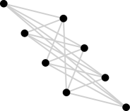
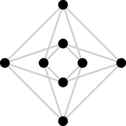
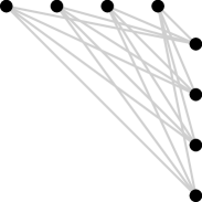
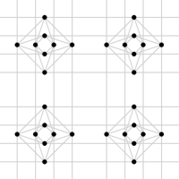
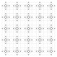
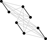
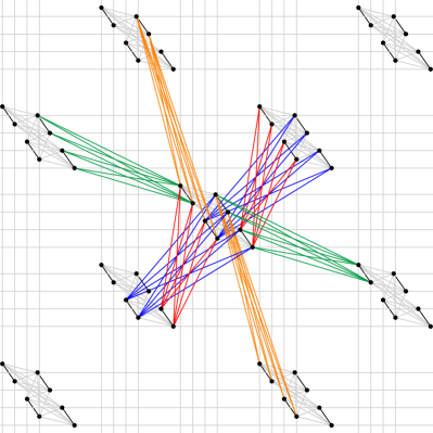
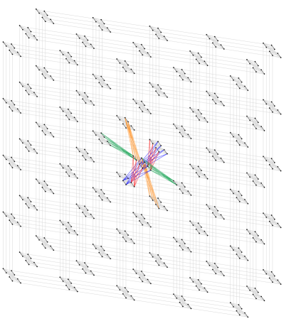
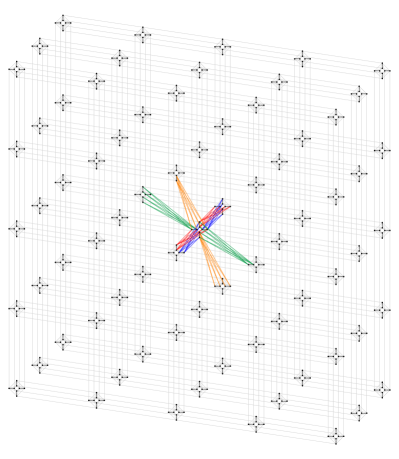
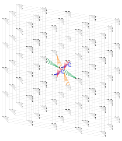
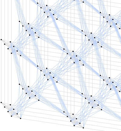
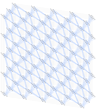
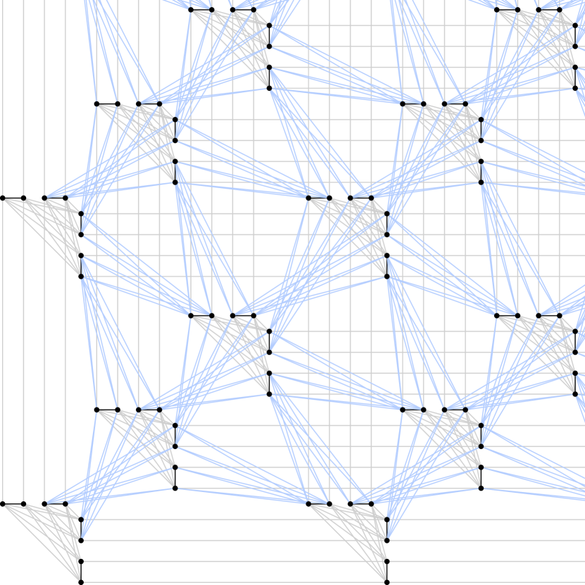
In all of the figures in this publication, the origin will be in the bottom-left corner, the index will increase in the right-hand direction, the index will increase in the upward direction, and the index (which indicates which Chimera layer is being considered) will increase in the direction going upward and rightward simultaneously (since paper and computer screens are still two-dimensional), see Figure 2a. Then will represent the left side in the classic depiction, or the horizontal vertices in the diamond-shaped or triangle-shaped depictions; while will represent the right side in the classic and vertical vertices in the diamond and triangle.
| Index | Range | Description |
|---|---|---|
| to | Row within a Chimera layer | |
| to | Column within a Chimera layer | |
| to | Chimera layer | |
| ‘Side’ within | ||
| First index within each ‘side’ of | ||
| Second index within each ‘side’ of |
I.2 The edges (couplings) in Chimera
I.2.1 Edges forming each cell
The cells are given by:
| (1) |
This means for each cell, all vertices for side are coupled to all vertices of side . For this entire publication, can be equal to or different from (and likewise for and ).
I.2.2 Edges connecting different cells
The horizontal lines between cells in Figure 1 can be described by adding 1 to while keeping all other variables constant and setting :
| (2) |
and the vertical lines can be described by adding 1 to while keeping all other variables constant and setting :
I.3 The new edges (couplings) in Pegasus
I.3.1 New edges added to each cell:
Pegasus first adds connections within each cell, given by simply coupling each vertex labeled as to its counterpart with all other variables unchanged:
| (4) |
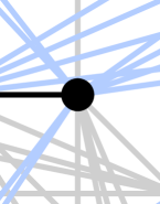
These edges are drawn black in the figures.
I.3.2 Edges connecting different cells:
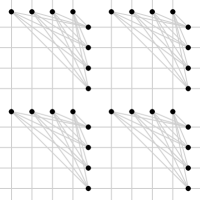
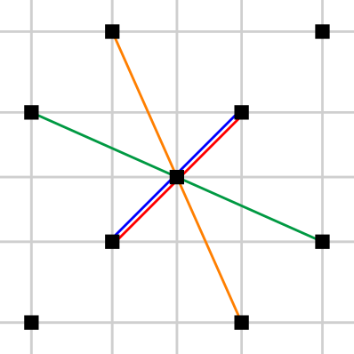
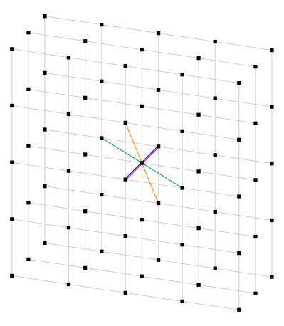
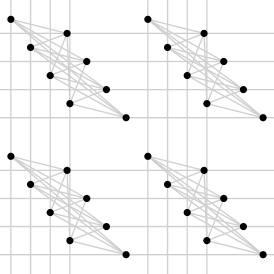
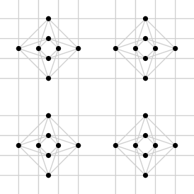
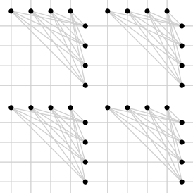
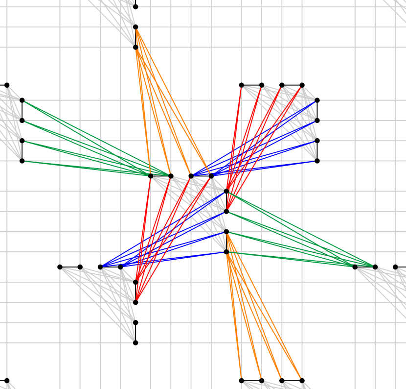
The rest of the new connections in Pegasus come from connecting the cells between different layers (different ) of Chimera graphs. The qubits of a cell located at coordinates will be connected to different cells on the other Chimera layers, with 64 edges in the form of 8 different graphs: 1 graph (8 edges) for each of 4 different connecting cells, and 2 graphs (16 edges) for the other 2 connecting cells.
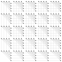
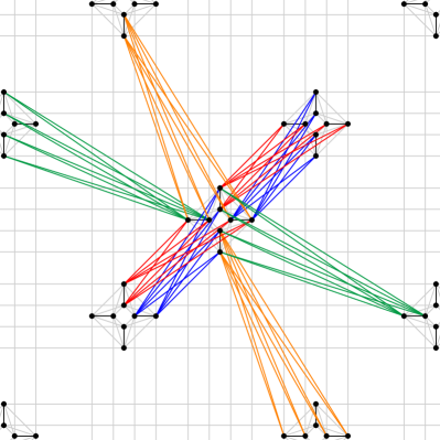
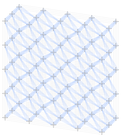
Figure 2b shows these 64 edges, and the 8 groups of 8-edge graphs connecting the central cell to 6 others are shown with 4 different colors. This is because we have found a set of 4 convenient rules that can be repeated to generate the entire Pegasus graph, and it is found that 4 of the graphs can be generated by applying these 4 rules to the central cell, and the other 4 of the graphs can be generated by applying these 4 rules to other cells (or by applying the 4 rules to the central cell again, but in reverse). We will now describe the rules.
First, all edges are between vertices of one side and its complementary side in a different (so vertices are coupled to vertices of a in a different layer). In fact all connections will be of the form where and can be any value in . All edges can actually be described using just a one-line rule:
| (5) |
For the layers labeled or 1 (meaning that , we have:
| (6) |
Substituting into Eq. (6) tells us that all vertices of a cell are connected to all vertices of the opposite side in the cell with the same , but in the next layer :
| (7) |
Substituting into Eq. (6) tells us that all vertices are also connected to all and vertices in the opposite side in a cell in the next layer , but with and coordinates shifted by 1 in the following way:
| (8) |
For the layer (, we have from Eq. (5):
| (9) |
Substituting into Eq. (9) tells us that all vertices of a cell are connected to the cells in the layer, but with and coordinates both shifted by 1:
| (10) |
Substituting into Eq. (9) tells us that all vertices are connected in the following way:
| (11) |
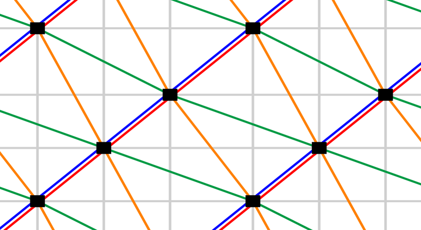
We now explicitly write down the 4 rules which lead to the grouping scheme depicted in Figure 2b (these rules are different depending on whether or , so there are actually 8 relations):
| (12) | ||||
| (13) | ||||
| (14) | ||||
| (15) | ||||
| (16) | ||||
| (17) | ||||
| (18) | ||||
| (19) |
II Comparison to Chimera
II.1 Degree of the vertices
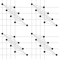
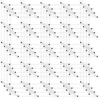
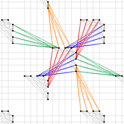
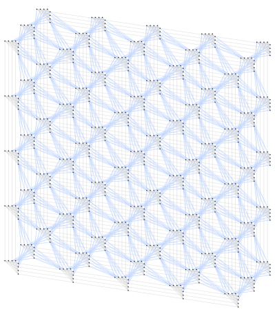
If we look for example at the cell at position in Fig. 2a, we can find that vertices have a degree of fifteen: The 6 grey edges that would regularly be in Chimera (4 to form the cell and 2 to connect to cells above/left and below/right), then there is 1 Pegasus edge added within one cell according to Eq. (4), then we have 8 more Pegasus edges for connecting cells of different Chimera layers , from Eqs. (12)-(15) (or from Eqs. (16)-(19) if we were starting with a cell in the layer). Therefore the degree (which is 15) has increased by a factor of 2.5 when compared to the degree of Chimera (which is 6).
In Fig. 2a, the cells at the boundary, such as at position , do not show a degree of 15, just as the cells of Chimera at the boundary would not show a degree of 6.
II.2 Non-planarity
We note that certain binary optimization problems forming planar graphs can be solved on a classical computer with a number of operations that scales polynomially with the number of binary variables, with the blossom algorithm Edmonds (1965a); *Edmonds1965a. Therefore it is important that the qubits of a quantum annealer are connected by a non-planar graph. The cells of Chimera are already sufficient to make all commercial D-Wave annealers non-planar. However, if each cell of a Chimera’s physical qubits were to encode just one logical qubit (in for example, an extreme case of minor embedding), then Chimera would be planar. While all added edges in Pegasus that connect different Chimera layers are of the form , which itself is planar; these edges connect cells of different planes of chimeras in a non-planar way, such that even if each cell were to represent one logical qubit, these logical qubits would still form a non-planar graph in Pegasus. This should expand the number of binary optimization problems that cannot yet be solved in polynomially time, that can potentially be embedded onto a D-Wave annealer.
II.3 Embedding
We have written an entire paper on the minor-embedding of quadratization (Dattani, 2019) gadgets onto Chimera and Pegasus (Dattani and Chancellor, 2019). One highlight of that work is the fact that all quadratization gadgets for single cubic terms which require one auxiliary qubit, can be embedded onto Pegasus with no further auxiliary qubits because Pegasus contains which means that all three logical qubits and the auxiliary qubit can be connected in any way, without any minor-embedding. We refer the reader to that paper (Dattani and Chancellor, 2019) for more thorough details about the advantage of Pegasus over Chimera for the minor-embedding of quadratization gadgets.
III Open source code for generation of Pegasus figures
All figures in this publication and its supplemental material can be generated (in vector graphic form) using our open source and customizable code which should be cited as Ref. (Szalay et al., 2018). The user can choose which type of Pegasus graph; the dimensions and ; the edge colors and widths, the vertex colors and widths; among other things (see the manual to Ref. (Szalay et al., 2018) for details).
Acknowledgments
We gratefully thank Kelly Boothby of D-Wave for her time spent in verifying the correctness of our algorithm. NC was funded by EPSRC (Project: EP/S00114X); SzSz by the NRDIF (NKFIH-K120569 and Quantum Technology National Excellence Program 2017-1.2.1-NKP-2017-00001) and the HAS (János Bolyai Research Scholarship and “Lendület” Program).
References
- Neven et al. (2009) H. Neven, V. S. Denchev, M. Drew-Brook, J. Zhang, W. G. Macready, and G. Rose, NIPS 2009 Demonstration: Binary Classification using Hardware Implementation of Quantum Annealing, Tech. Rep. (2009).
- Edmonds (1965a) J. Edmonds, Canadian Journal of Mathematics 17, 449 (1965a).
- Edmonds (1965b) J. Edmonds, Journal of Research of the National Bureau of Standards-B., Tech. Rep. 2 (1965).
- Dattani (2019) N. Dattani, Quadratization in discrete optimization and quantum mechanics (2019) arXiv:1901.04405 .
- Dattani and Chancellor (2019) N. Dattani and N. Chancellor, (2019), .
- Szalay et al. (2018) S. Szalay, N. Dattani, and N. Chancellor, (2018), https://github.com/HPQC-LABS/PegasusDraw, DOI: 10.5281/zenodo1953876.
Supplementary Material