Magnetic stripe soliton and localized stripe wave in spin-1 Bose-Einstein condensates

Abstract

The recent experimental realization of spin-orbit coupling for ultracold atomic gases opens a new avenue for engineering solitons with internal spatial structures through tuning atomic band dispersions. However, the types of the resulting stripe solitons in a spin-1/2 Bose-Einstein condensate (BEC) have been limited to dark-dark or bright-bright with the same density profiles for different spins. Here we propose that general types of stripe solitons, including magnetic stripe (e.g., dark-bright) and localized stripe waves (neither bright nor dark), could be realized in a spin-1 BEC with widely tunable band dispersions through modulating the coupling between three spin states and the linear momentum of atoms.  Surprisingly, a moving magnetic stripe soliton can possess both negative and positive effective masses at different velocities, leading to a zero mass soliton at certain velocity. Our work showcases the great potential of realizing novel types of solitons through band dispersion engineering, which may provide a new approach for exploring soliton physics in many physical branches.

Introduction: Solitons are topological defects that play significant roles in many different physical branches, such as water waves, fiber optics, and nonlinear matter waves S2 ; Drazin ; Dickey ; Kivshar ; S6 . Ultra-cold atomic superfluids, such as Bose-Einstein condensates (BECs) and degenerate Fermi gases (DFGs), provide a disorder-free and highly controllable platform for exploring soliton physics Denschlag ; Anderson ; fermib ; Meyer ; S5 ; S7 ; BS ; S8 ; S4 ; BEC ; Ebd ; Bersano . In particular, because solitons arise from the interplay between band dispersion and nonlinearity, tuning atomic interactions through Feshbach resonance RevModPhys.82.1225 provides a tunable knob for generating various types of solitons and exploring their dynamical properties. For instance, a dark (bright) soliton has been observed in a single component BEC with repulsive (attractive) interaction S5 ; S7 ; BS , while their combinations, such as dark-dark and dark-bright solitons have been realized in multiple-component BECs with different inter- and intra-component interactions S4 ; BEC ; Ebd . Notably, a “magnetic soliton” with a uniform total atom density has been predicted recently for a two-component BEC Qu1 ; Qu2 , where the dark soliton of one component is perfectly filled by the anti-dark soliton of the other component.

The recent experimental realization of spin-orbit coupling for ultracold atoms lin2011spin ; zhang2012collective ; qu2013observation ; olson2014tunable ; wang2012spin ; Cheuk2012 ; Williams2013 ; huang2016experimental ; wu2016realization ; campbell2015itinerant ; luo2016tunable opens a new avenue for exploring soliton physics through engineering atomic band dispersions Fialko ; Zhou ; Kartashov ; stripeso ; Wu ; Xu ; Achilleos ; stripeso2 . In a spin-1/2 BEC, the spin-orbit coupling displays a double well band dispersion, and the simultaneous occupation of two momentum space minima opens the possibility for generating solitons with internal spatial structures, i.e., the stripe density modulation stripeso ; Wu ; Xu ; Achilleos ; stripeso2 . However, the intrinsic Raman coupling for the realization of spin-orbit coupling mixes two spin states, which demands the same spatial density for different spins, therefore only certain types of stripe solitons such as bright-bright or dark-dark can exist stripeso ; Wu ; Xu ; Achilleos ; stripeso2 . A natural question is whether general types of stripe solitons, such as magnetic stripe solitons (dark-bright or dark-antidark types) could be generated by tuning the band dispersion beyond that for spin-1/2 spin-orbit coupling.

In this paper, we address this important question by considering a spin-1 BEC with widely tunable band dispersion achieved by coupling three spin states $\left\{\left|\uparrow\right\rangle,\left|0\right\rangle,\left|\downarrow\right\rangle\right\}$ with the linear momentum of atoms. Our main results are:

i) Both dark-bright and dark-antidark stripe solitons could exist for ferromagnetic or antiferromagnetic spin interactions. The dark and bright solitons reside at two band minima with different momenta and the spin states $\left|\uparrow\right\rangle$ and $\left|\downarrow\right\rangle$ exhibit strong stripe density modulations on top of a soliton background.

ii) By slightly tuning the spin interactions, a magnetic stripe soliton with a uniform total density could be generated. The dark-soliton dip in the state $|0\rangle$ is perfectly filled by the bright-soliton atoms in states $\left|\uparrow\right\rangle$ and $\left|\downarrow\right\rangle$, which exhibit an out-of-phase density modulation. More interestingly, the soliton’s effective mass can possess both positive and negative values at different velocities, in contrast to solitons with a fixed sign of mass in previous literature Qu1 ; eff1 ; eff2 ; eff3 ; eff4 ; Scott .

iii) When the spin interaction is comparable with the density interaction, a localized stripe wave for states $\left|\uparrow\right\rangle$ and $\left|\downarrow\right\rangle$, which is neither bright nor dark, could exist. Two local stripe density modulations reside on the same uniform background, but cancel each other, leading to a uniform spin tensor density.

iv) Such magnetic stripe solitons and localized stripe waves are stable and their stability is confirmed by numerically simulating the mean-field dynamical equations.

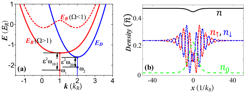
Figure 1: (a) Single-particle band structures with detuning $\Delta=-\delta=-0.8$. The red solid (dashed) line denotes the bright band for $\Omega=1.2$ ($\Omega=0.4$), and the blue line denotes the dark band (independent of $\Omega$). The $\epsilon^{2}\omega_{j0}$ $(j=1,2)$ corresponds to the nonlinear energy correction induced by the soliton. (b) The spin-density distributions for a typical stripe soliton solution with anti-ferromagnetic interaction $g_{2}>0$. $n$ is the total density. The parameters are $\epsilon=0.1$, $g_{2}=-0.1$, $g_{0}=1$, $\delta=0.5$, $\omega_{10}=-42.75$, $\omega_{20}=-47.5$.

System and methods: We consider the emergence of stripe solitons on two spin states $\left|\uparrow\right\rangle$ and $\left|\downarrow\right\rangle$ through their coupling with the third state $\left|0\right\rangle$ in a spin-1 BEC. To avoid large momentum transfer between $\left|\uparrow\right\rangle$ and $\left|\downarrow\right\rangle$, while still modify their local band dispersions, we adopt the recently proposed spin-tensor-momentum coupling for a spin-1 system Luo ; Luo2 , which can be realized by coupling three hyperfine ground states (denoted as $\{\left|\uparrow\right\rangle,\left|0\right\rangle,\left|\downarrow\right\rangle\}$) of Alkali atoms through Raman and microwave transitions [similar scheme also applies to alkali-earth(-like) atoms]. The single-particle Hamiltonian under the basis $\{\left|\uparrow\right\rangle,\left|0\right\rangle,\left|\downarrow\right\rangle\}$ reads

$$H_{0}=(i\partial_{x}+2F_{z}^{2})^{2}+\Delta F_{z}^{2}+\sqrt{2}\Omega F_{x}+\delta(\left|\uparrow\right\rangle\left\langle\downarrow\right|+h.c.).$$ (1)

Here we set $\hbar=1$ and the recoil energy $E_{R}=k_{R}^{2}/2m$ and momentum $k_{R}$ as energy and momentum units. $F_{z}$ and $F_{x}$ are spin-1 vectors, $\Delta$ is the tensor Zeeman field, $\Omega$ is the Raman coupling strength between states $\left|\uparrow,\downarrow\right\rangle$ and $\left|0\right\rangle$, and $\delta$ describes the microwave coupling between $\left|\uparrow\right\rangle$ and $\left|\downarrow\right\rangle$. The typical lower band structure is shown in Fig. 1(a), with the low energy dynamics characterized by two bands: the dark band $E_{D}(k)$ (blue line) for the state $\left|-\right\rangle$; the bright band $E_{B}(k)$ (red lines) for the mixture of the states $\left|+\right\rangle$ and $\left|0\right\rangle$, where $\left|\pm\right\rangle=\frac{1}{\sqrt{2}}(\left|\uparrow\right\rangle\pm\left|\downarrow\right\rangle)$). The dark band has a minimum at $k=2$, while the bright band may have one or two band minima depending on the Raman coupling strength $\Omega$.

The interaction between atoms, which is needed for generating solitons, can be described under the mean field approximation. For the simplicity of the calculation, the spin basis $\{\left|+\right\rangle,\left|0\right\rangle,\left|-\right\rangle\}$ is used with the corresponding mean-field Gross-Pitaevskii equation (see Appendix)

$$i\partial_{t}\psi_{j}=H_{0}\psi_{j}+(g_{0}\bar{n}+g_{2}\bar{n})n\psi_{j}-g_{2}|\psi_{j}|^{2}\psi_{j}+\delta_{j,0}\gamma|\psi_{j}|^{2}\psi_{j},$$ (2)

where $\psi_{j}$ is the wavefunction at the spin state $|j\rangle$, $g_{2}$ and $g_{0}>|g_{2}|$ are the spin and density interaction strengths, respectively, and $n$ is the atom density with density unit $\bar{n}$ (we set $\bar{n}=1$ without loss of generality). The term $\delta_{j,0}\gamma|\psi_{j}|^{2}\psi_{j}$ in the right-hand side of Eq. 2 corresponds to additional intra-component interaction $\frac{\gamma}{2}|\psi_{0}|^{4}$ for spin state $\left|0\right\rangle$, which can be realized using Feshbach resonance RevModPhys.82.1225 . Hereafter $\Delta=-\delta$ is chosen so that the bright band is symmetric around $k=1$ to obtain simple analytic soliton solutions.

Since exact analytic soliton solutions cannot be obtained for such a spin-1 system, here we derive an approximate solution using the multi-scale expansion method stripeso ; stripeso2 . We choose an ansatz for the wavefunctions of the soliton

$$\psi_{+(0)}=A_{+(0)}\left(x\right)e^{ik_{1}x-i\omega_{1}t},\text{ }\psi_{-}=A_{-}\left(x\right)e^{ik_{2}x-i\omega_{2}t},$$ (3)

where $A_{+}$, $A_{0}$ and $A_{-}$ (with $|A_{j}|\ll 1$) describe the spatial profiles of the soliton, $k_{1}$, $k_{2}$ are the center momenta of the soliton, and $\omega_{1}$, $\omega_{2}$ are the soliton energies. The soliton amplitudes can be expanded as $A_{j}=\sum_{\eta}\epsilon^{\eta+1}\chi_{j}^{(\eta)}$ using a small parameter $\epsilon$, where $\chi_{j}^{(\eta)}$ are slowly varying functions (i.e. $\partial_{x}\chi_{j}^{(\eta)}\sim\epsilon\chi_{j}^{(\eta)}$). Substituting the ansatz (3) into Eq. (2), we obtain the soliton solution and corresponding constrains on $\chi_{j}^{(\eta)}$ according to the solvability conditions up to the order of $O(\epsilon^{3})$. It is easy to check that the leading order solution satisfies $\chi_{+}^{(0)}=-\chi_{0}^{(0)}\equiv U(X)$ and $\chi_{-}^{(0)}\equiv V(X)$ with $X=\epsilon x$.

Dark-bright stripe soliton: Here we focus on the case $\Omega=1$ where the bright band has a minimum at $k=1$ and the dispersion effects are suppressed significantly. The soliton solution is static with $k_{1}=1$, $k_{2}=2$. The leading order in the wavefunction (3) yields $A_{+}\left(x\right)=-A_{0}\left(x\right)\approx\epsilon U(X)$, $A_{-}\left(x\right)=\epsilon V(X)$, $\omega_{1}\approx E_{B}(1)-\epsilon^{2}\omega_{10}$, and $\omega_{2}\approx E_{D}(2)-\epsilon^{2}\omega_{20}$, with the energy corrections $\epsilon^{2}\omega_{10}$ and $\epsilon^{2}\omega_{20}$ induced by the nonlinear interaction. For $\gamma=0$, the mean-field equation (2) can be approximated as

$$\partial_{X}^{2}V(X)+g_{V}|V(X)|^{2}V(X)+w_{V}V(X)=0,$$ (4)

where the coefficients $g_{V}=\left(2g_{2}^{2}+3g_{0}g_{2}\right)/\left(2g_{0}+g_{2}\right)$ and $w_{V}=2(g_{0}+g_{2})\omega_{10}/\left(2g_{0}+g_{2}\right)-\omega_{20}$. $U(X)$ can be determined through the constrain

$$|U(X)|^{2}+\frac{g_{0}+g_{2}}{2g_{0}+g_{2}}|V(X)|^{2}=\frac{-\omega_{10}}{2g_{0}+g_{2}}>0.$$ (5)

Since $g_{V}$ has the same sign as $g_{2}$, the effective interaction strength $g_{V}<0$ or $g_{V}>0$ in Eq. (4) for ferromagnetic ($g_{2}<0$) and antiferromagnetic ($g_{2}>0$) spin interactions, respectively. For $g_{V}<0$, Eqs. (4) and (5) have a dark soliton solution

$$V(X)=\sqrt{\frac{w_{V}}{-g_{V}}}\tanh[\sqrt{\frac{w_{V}}{2}}X]$$ (6)

in the parameter region $\frac{g_{0}+g_{2}}{g_{V}}\geq\frac{\omega_{10}}{\omega_{V}}$ and $w_{V}>0$. The corresponding $U$ from Eq. (5) is a bright or anti-dark soliton. While for $g_{V}>0$,

$$V(X)=\sqrt{\frac{-2w_{V}}{g_{V}}}\operatorname{sech}[\sqrt{-w_{V}}X]$$ (7)

is a bright soliton in the parameter region $\frac{g_{0}+g_{2}}{g_{V}}\leq\frac{\omega_{10}}{2\omega_{V}}$ and $w_{V}<0$, and $U$ is a dark soliton. Such dark-bright solution at two band minima is different from previous bright-bright or dark-dark soliton solutions in a spin-1/2 BEC stripeso ; Wu ; Xu ; Achilleos . The stripe solitons for spin states $\left|\uparrow\right\rangle$ and $\left|\downarrow\right\rangle$ are formed by the superposition of such bright-dark solitons at two band minima, leading to strong out-of-phase density modulations for two states, as shown in Fig. 1(b). The total density $n\equiv 2|U|^{2}+|V|^{2}=\frac{-2\omega_{10}}{2g_{0}+g_{2}}-\frac{g_{2}}{2g_{0}+g_{2}}|V|^{2}$ possesses a weak soliton profile ($\sim|V|^{2}$) on top of a uniform background $\frac{-2\omega_{10}}{2g_{0}+g_{2}}$ [see Fig. 1(b)]. Similar types of solitons also exist for $\Omega>1$ although analytic solutions are hard to obtain.

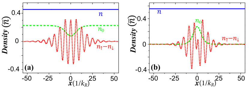
Figure 2: (a) and (b) The spin-density distributions for the magnetic stripe soliton with $g_{2}>0$ and $g_{2}<0$, respectively. The total density is uniform, while the spin density $\mathcal{F}_{z}=n_{\uparrow}-n_{\downarrow}$ exhibits stripe modulation. The parameters are $g_{2}=0.1$, $\omega_{20}=-48.5$ for (a) and $g_{2}=-0.1$, $\omega_{20}=-\frac{g_{0}}{g_{0}+g_{2}}\omega_{10}$ for (b) with other parameters $\epsilon=0.1$, $g_{0}=1$, $\gamma=2g_{2}$, $\Omega=1$, $\omega_{10}=-50$, $\delta=0.5$.

Magnetic stripe solitons— For typical nonlinear interactions in Eq. 2 with $\gamma=0$, the dark soliton dip cannot be perfectly filled by the bright soliton particles, leading to a small dip for the total density. We note that it is possible to construct the magnetic stripe soliton with the uniform total density, with $\gamma\neq 0$.

For $\Omega=1$, the soliton solution is still static and $V$ takes the same form (6) or (7) as that for $\gamma=0$, except that $g_{V}$ and $\omega_{V}$ change to $g_{V}=\frac{2g_{2}^{2}+3g_{0}g_{2}-g_{0}\gamma/2}{2g_{0}+g_{2}+\frac{\gamma}{2}}$, $w_{V}=\frac{2(g_{0}+g_{2})\omega_{10}}{2g_{0}+g_{2}+\frac{\gamma}{2}}-\omega_{20}$. Eq. (5) for determining $U$ is modified by replacing $2g_{0}+g_{2}$ in the denominator with $2g_{0}+g_{2}+\gamma/2$. The total density is $n=\frac{-2\omega_{10}}{2g_{0}+g_{2}+\gamma/2}-\frac{g_{2}-\gamma/2}{2g_{0}+g_{2}+\gamma/2}|V|^{2}$, which becomes uniform when $\gamma=2g_{2}$. The spin-density profiles for the magnetic stripe soliton with (anti-)ferromagnetic interaction $g_{2}<0$ ($g_{2}>0$) are shown in Figs. 2(a) and 2(b). While the total density is uniform, the spin density $\mathcal{F}_{z}=n_{\uparrow}-n_{\downarrow}$ exists stripe density modulation. For $g_{2}<0$, the magnetic stripe soliton may be formed either by dark and bright solitons or by dark and anti-dark solitons, while the latter may have striped spin background (see Appendix).

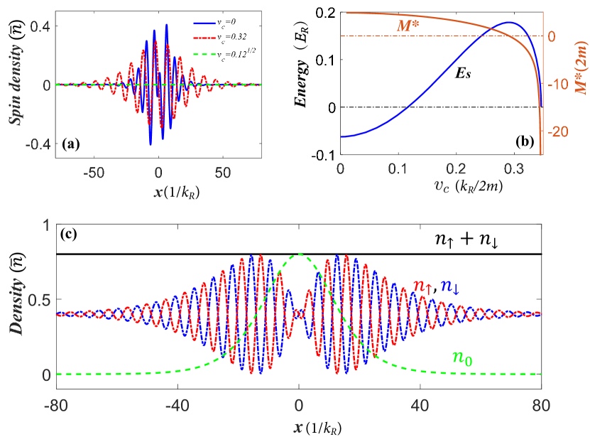
Figure 3: (a) The moving magnetic stripe soliton profiles at different velocities. (b) The energy $E_{s}$ (blue line) and effective mass $M^{\ast}=\frac{\partial E_{s}}{\partial v_{c}^{2}}$ (red line) of the magnetic stripe soliton versus its velocity. Other parameters for (a) and (b) are $\epsilon=0.1$, $g_{2}=-0.1$, $g_{0}=1$, $\Omega=2$, $\gamma=4g_{2}$, $C=60$, $\delta=1.5055$. (c) Density profiles for localized stripe waves. The spin tensor density $\mathcal{F}_{z}^{2}=n_{\uparrow}+n_{\downarrow}$ is a constant. The parameters are $\epsilon=0.1$, $g_{2}=-0.1$, $g_{0}=0.19$, $\Omega=1$, $\gamma=-2g_{0}$, $\omega_{10}=-7.2$, $\omega_{20}=\frac{g_{0}}{g_{0}+g_{2}}\omega_{10}$, $\delta=0.5$.

For $\Omega>1$, the general soliton solution for an arbitrary $\gamma$ is not easy to obtain. However, the magnetic stripe soliton with a constant total density $n=C$, which requires $\gamma=g_{2}(6-\frac{4}{\Omega})$, can be obtained analytically. Such magnetic stripe soliton for $\Omega>1$ can have a finite velocity, with the wave function

$$U(X,T) = \sqrt{\frac{n_{v}}{2}}\operatorname{sech}[f(X-vT)]\exp(i\delta kX),$$ (8)

$$V(X,T) = \sqrt{n_{v}}\tanh[f(X-vT)]+\frac{iv}{\sqrt{2C|g_{2}|}}$$ (9)

for $g_{2}<0$. Here $f(X-vT)=\sqrt{|g_{2}|n_{v}}(X-vT)$, $n_{v}=C+\frac{v^{2}}{2g_{2}}$, and $\delta k=\frac{\Omega v}{2(\Omega-1)}$ corresponds to a small derivation of the center momentum away from the band minimum. Notice that the solution is valid only when $\Omega$ is not so close to 1 to ensure a small $\delta k$. $T=\epsilon^{2}t$ describes the slowly varying time, and the velocity parameter $v\leq\sqrt{2C|g_{2}|}$ should be always less than the sound speed of the background. The soliton energies induced by the nonlinear interaction read $\omega_{10}=-g_{0}C-g_{2}C\frac{3\Omega-1}{2\Omega}-v^{2}\frac{2\Omega^{2}-2\Omega+1}{4\Omega(\Omega-1)}$, and $\omega_{20}=-g_{0}C$. Such magnetic stripe soliton has a velocity $v_{c}=\epsilon v$ with respect to the static particle density background. The profile of the magnetic stripe soliton depends on its velocity: the peak value decreases while its spatial width increases with the velocity [as shown in Fig. 3 (a)]. Similar soliton solutions can be obtained for $g_{2}>0$.

The moving soliton usually can be described as an quasiparticle with an effective mass and energy. The energy $E_{s}$ of the soliton is defined as the difference between the grand canonical energies in the presence and absence of the soliton (with the same particle density background), while the effective mass $M^{\ast}=\frac{\partial E_{s}}{\partial(v_{c}^{2})}$ Qu1 ; Scott is determined accordingly. In Fig. 3 (b), the energy and effective mass of the moving stripe soliton are plotted versus its velocity. The energy increases first and then decreases as the velocity increases, while the effective mass possesses both negative and positive values and crosses zero at a velocity smaller than the sound speed. Close to the sound speed, the effective mass approaches infinity due to the velocity dependence of the dark-bright soliton profiles. These characters, especially the zero mass at a velocity less than the sound speed, are in sharp contrast to bright or dark solitons with a fixed sign of mass in previous studies eff1 ; eff2 ; eff3 ; eff4 ; Scott . Recently, the positive mass and negative mass of soliton was discussed in a spin-orbit coupled BEC stripeso2 , which is induced by the effective mass of single atom (single-particle band dispersion). The negative mass of magnetic stripe soliton is mainly induced by the nonlinearity instead of the single-particle band dispersion. Therefore, the magnetic stripe soliton can admit negative mass even though the effective single-particle mass is positive, leading to very unique properties such as the infinity and zero mass at different velocities. We note that similar tunable inertial mass of atomic Josephson vortices and related solitary waves can also be achieved through an adjustable linear coupling between the two components in a BEC Brand . These striking inertial mass properties could inspire more discussions on the dispersion relation of quasi-particle nonlinear waves.

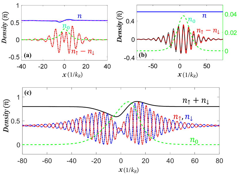
Figure 4: (a) and (b) Numerical simulations for the magnetic stripe solitons in Fig. 2(b) and Fig. 3(b). (c) Numerical simulation for the localized stripe wave in Fig. 3(c). The evolution time is $t=20$. The solitons are stable and the high order corrections are negligible in (a) and (b) but more significant for (c). The thin purple dashed line in (a) is the initial total density, and the thin black solid line in (b) is the initial stripe density modulation.

Localized stripe wave— In stripe solitons discussed in either spin-1/2 BEC stripeso ; Wu ; Xu ; Achilleos ; stripeso2 or above magnetic stripe soliton, the striped density modulation resides on a bright or dark soliton background. Here such density background is given by $|U|^{2}+|V|^{2}$, which can be tuned to be uniform by the spin-dependent interaction $\gamma$, therefore the stripe soliton for states $\left|\uparrow\right\rangle\$and $\left|\downarrow\right\rangle$ is neither bright nor dark, but a localized stripe wave. For instance, when $\Omega=1$, $\gamma=-2g_{0}$, the spin tensor density $\mathcal{F}_{z}^{2}=n_{\uparrow}+n_{\downarrow}$ becomes uniform. For $g_{2}>0$ ($g_{2}<0$), the localized stripe waves for states $\left|\uparrow\right\rangle\$and $\left|\downarrow\right\rangle$ exists for $\frac{2w_{V}}{g_{V}}\leq\frac{-\omega_{10}}{g_{0}+g_{2}}$ ($\frac{w_{V}}{|g_{V}|}=\frac{-\omega_{10}}{g_{0}+g_{2}}$), while the state $|0\rangle$ admits a dark (bright) soliton profile, as shown in Fig. 3(c).

Stability of solitons— To check the stability of these stripe solitons obtained from the multi-scale expansion method, we numerically simulate the time evolution dynamics of the obtained solitons using the GP equation (2) with the analytic soliton solutions as the initial states. As an example, we consider the magnetic stripe solitons for ferromagnetic interaction ($g_{2}<0$). Both static [$\Omega=1$ in Fig. 2(b)] and moving [$\Omega>1$ and $v_{c}=0.32$ in Fig. 3(a)] solitons are found to be stable [see Fig. 4(a) and (b)]. We notice that higher order terms in the solution may induce slight modulation of the soliton profile, which is typically of the order of $\epsilon^{2}$. In addition, a nonzero $\gamma$ breaks the balance between state $|+\rangle$ and $|0\rangle$, leading to small atom transitions between them. However, as long as $\gamma$ is weak compared with the density interaction $g_{0}$, such transitions hardly affect the stability of the soliton and the uniformity of the total density.

The localized stripe wave requires a $\gamma$ that is comparable with $g_{0}$, yielding a strong coupling between states $|+\rangle$ and $|0\rangle$. Nevertheless, we find that stable solitons can still exist when both $\gamma$ and $g_{0}$ are weak compared with the recoil energy. In Fig. 4(c), we show our numerical result with density interaction $g_{0}=1.9|g_{2}|$, $g_{2}<0$ and $\gamma=-2g_{0}$. Although the localized stripe wave is stable, the spin background $|U|^{2}+|V|^{2}$ is no longer uniform, but exhibits a soliton profile due to the nonzero $\gamma$ (which is comparable with $g_{0}$). The numerical simulations of the dark-bright stripe solitons with $\gamma=0$ are shown in the Appendix, which are in good agreement with Fig. 1(b) thanks to the absence of transitions between states $|+\rangle$ and $|0\rangle$.

Discussion and conclusion— The spin interaction $g_{2}$ (either $>0$ or $<0$) of alkaline atoms is usually much smaller than the density interaction $g_{0}$ PhysRevLett.81.742 ; Ohmi1998Bose ; RevModPhys.85.1191 . The intra-component interaction strength $\gamma$ for the state $\left|0\right\rangle$, can be realized by using an additional Feshbach resonance RevModPhys.82.1225 . In our simulation of the magnetic stripe soliton, we consider $g_{2}=\pm 0.1g_{0}$, and as we increase (decrease) $|g_{2}|$, the soliton properties would not be affected, except that its size may decrease (increase) slightly. Different from the ground-state stripe phase, the stripe solitons can exit in a large parameter region and the choice of $\Omega$ and $\Delta$ is very flexible. This is because the solitons are metastable states and we can have solutions even when the detuning between two (bright and dark) band minima are much larger than $g_{2}$. We focus our study in the $\Omega\geq 1$ region. For $\Omega<1$, the bright band has two band minima around $k=1$, and there still exist magnetic stripe soliton solutions with $k_{1}$ located at one of two band minima (see Appendix). In experiments, the soliton may be imprinted at the center of the BEC cloud using light-induced spatial dependent potential, and observed after some evolution time S8 ; Denschlag ; Anderson .

In summary, we demonstrate new types of stripe solitons, such as magnetic stripe solitons and localized stripe waves, can be engineered by tuning the band dispersion in a spin-1 BEC with spin-orbit coupling. These solitons are quite different from the solitons in the spin-orbit coupled BEC stripeso ; Wu ; Achilleos ; stripeso2 ; Kartashov , which further enrich soliton family in BEC and many other nonlinear systems and may be used for both fundamental studies (e.g., spin-orbital coupling, nonlinear effects, quantum fluctuations Kadau ; QF ; QF2 , modulational instability MI , quantum entanglement Gertjerenken ) and realistic applications (e.g., atomic soliton laser). The striking effective mass characters of these solitons may shed light on the study of particle physics MRN ; PAR . While many interesting problems, such as the generalization of magnetic stripe solitons to higher dimension Zhou ; Gautam ; Gallem ; Law , remain to be explored, our work clearly showcases the power of soliton generation through band dispersion engineering, which may provide a new approach for exploring soliton physics in many physical branches.

I Appendix

In the appendix, we derive the non-linear Schrödinger equation of the spin-1 system, and give the magnetic stripe soliton solutions in other parameter regions not shown in the main text.

I.0.1 Non-linear Schrödinger equation

In the Lab frame, the second-quantization Hamiltonian can be written as

$$\mathcal{H}=\int dx\Psi^{{\dagger}}H_{0}\Psi+\int dx\frac{g_{0}}{2}(\Psi^{{\dagger}}\Psi)^{2}+\frac{\gamma}{2}(\psi_{0}^{{\dagger}}\psi_{0})^{2}+\frac{g_{2}}{2}(\Psi^{{\dagger}}\mathbf{F}\Psi)^{2},$$

with spin operator $\mathbf{F}=(F_{x},F_{y},F_{z})$, and atom field $\Psi=(\psi_{\uparrow},\psi_{0},\psi_{\downarrow})$. The non-linear Schrödinger equation can be obtained by

$$i\partial_{t}\Psi=[\Psi,\mathcal{H}].$$

In the quasi-momentum frame, we have Luo

$$i\partial_{t}\psi_{j}=H_{0}\psi_{j}+(g_{0}\bar{n}+g_{2}\bar{n})n\psi_{j}-g_{2}|\psi_{j}|^{2}\psi_{j}+\delta_{j,0}\gamma|\psi_{j}|^{2}\psi_{j}+g_{2}\psi_{j}^{\ast}Q_{j}(x),$$

Where $j=\pm,0$ and $Q_{+}(x)=\psi_{-}^{2}+\psi_{0}^{2}e^{i4x}$, $Q_{-}(x)=\psi_{+}^{2}-\psi_{0}^{2}e^{i4x}$, $Q_{0}(x)=(\psi_{+}^{2}-\psi_{-}^{2})e^{-i4x}$. We are interested in the solutions with momenta centering at the band minima, while the last term involves couplings with higher momenta far away from the band minima, therefore its effects is negligible and can be omitted. This is also confirmed by our numerical simulation in Fig. A1, where the last term only induces tiny and fast spatial modulations without affecting the soliton profile.

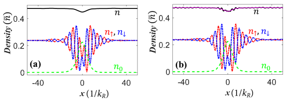
Figure A1: (a) and (b) Numerical results of the soliton profiles at $t=20$ without and with the $Q_{j}$ terms. The parameters are the same as those in Fig. 1b in the main text. The thin purple line in (b) is the total density without $Q_{j}$ term [same as the black line in (a)].

I.0.2 Dark-anti-dark magnetic stripe solitons

In the main text, we have focused on magnetic stripe solitons formed by dark and bright solitons, which admit spin-balanced background. However, at $\Omega=1$, the spin background can be imbalanced if it is formed by dark and anti-dark solitons. Such dark and anti-dark solitons can exist for ferromagnetic interactions $g_{2}<0$ with proper choice of parameters (i.e., $\omega_{10}$ and $\omega_{20}$), as shown in Fig. A2 (its stability is confirmed numerically). The soliton resides on a striped spin background, which is different from the stripe magnetic solitons with a zero spin background (as shown in Fig. 2 of the main text).

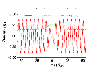
Figure A2: The spatial profiles of dark-anti-dark magnetic stripe soliton. The parameters are $\epsilon=0.1$, $g_{2}=-0.1$, $g_{0}=1$, $\omega_{10}=-50$, $\omega_{20}=-52.5$, $\delta=0.5$.

I.0.3 Magnetic stripe solitons for $\Omega<1$

For $\Omega<1$, the bright band has two minima at $k=1\pm\sqrt{1-\Omega^{2}}$, thus we expect to find stable stripe solitons by choosing the center momentum as $k_{1}=1\pm\sqrt{1-\Omega^{2}}$. Magnetic stripe solitons with a uniform total density require $\gamma=\frac{2g_{2}(3\Omega^{2}-4)(\Omega^{2}+2\sqrt{1-\Omega^{2}}-2)}{\Omega^{4}}$. As an example, we present a stripe soliton solution for $g_{2}<0$ and $k_{1}=1-\sqrt{1-\Omega^{2}}$, while similar soliton solutions can be obtained in other parameter regimes. The stripe magnetic soliton wavefunctions are $\psi_{\uparrow}\approx\frac{1}{\sqrt{2}}\epsilon[\frac{\sqrt{1-\Omega^{2}}-1}{\Omega}U(X,T)e^{ik_{1}x-i\omega_{1}t}+V(X,T)e^{ik_{2}x-i\omega_{2}t}]$ , $\psi_{0}\approx\epsilon U(X,T)e^{ik_{1}x-i\omega_{1}t}$, and $\psi_{\downarrow}\approx\frac{1}{\sqrt{2}}\epsilon[\frac{\sqrt{1-\Omega^{2}}-1}{\Omega}U(X,T)e^{ik_{1}x-i\omega_{1}t}-V(X,T)e^{ik_{2}x-i\omega_{2}t}]$, where $U(X,T)$ and $V(X,T)$ are

$$U(X,T) = \sqrt{\frac{p}{\gamma_{r}}}\operatorname{sech}[\sqrt{\frac{p}{2}}(X-vT)]\exp\left(-\frac{iT_{1}[n_{1}(g_{0}+g_{2})+\omega_{10}]}{1-\Omega^{2}}+\frac{ipT_{1}}{2}-\frac{1}{4}iT_{1}v_{1}^{2}+\frac{iv_{1}X}{2}\right),$$ (A1)

$$V(X,T) = \sqrt{n_{1}}[\sqrt{1-\frac{v^{2}}{2(-g_{2})n_{1}}}\tanh[\sqrt{\frac{1}{2}(-g_{2})n_{1}}\sqrt{1-\frac{v^{2}}{2(-g_{2})n_{1}}}(X-vT)]+\frac{iv}{\sqrt{2(-g_{2})n_{1}}}]\exp[i\phi],$$ (A2)

with $\gamma_{r}=\frac{\frac{g_{2}(2-\Omega^{2})(1-\sqrt{1-\Omega^{2}})}{\Omega^{2}}-\frac{1}{2}\gamma(\sqrt{1-\Omega^{2}}+1)}{1-\Omega^{2}}$, $p=\frac{1}{2}(-2g_{2}n_{1}-v^{2})$, $v_{1}=\frac{v}{1-\Omega^{2}}$, $T_{1}=(1-\Omega^{2})T$, and $\phi=g_{2}n_{1}T-n_{1}(g_{0}+g_{2})T+\omega_{20}T$.

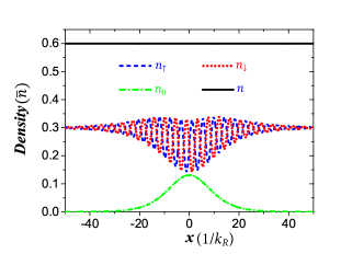
Figure A3: The magnetic stripe soliton for $\Omega<1$ and $g_{2}<0$. Numerical test shows that it is stable. The center momentum is $k_{1}=1-\sqrt{1-\Omega^{2}}$, and the additional spin-dependent modulation coefficient is $\gamma=\frac{2g_{2}(3\Omega^{2}-4)(\Omega^{2}+2\sqrt{1-\Omega^{2}}-2)}{\Omega^{4}}$. Other parameters are $\epsilon=0.1$, $g_{2}=-0.1$, $g_{0}=1$, $\Omega=2/3$, $n_{1}=60$, $\omega_{10}=0$, $\omega_{20}=0$, $\delta=4/18$, $v=3$.

Fig. A3 shows the typical density (spin) profiles of such solitons. The soliton is confirmed to be stable in the GP equation simulation, although higher order terms in the solution may induce minor distortion.