Speech Separation Using Gain-Adapted Factorial Hidden Markov Models

Abstract

We present a new probabilistic graphical model which generalizes factorial hidden Markov models (FHMM) for the problem of single channel speech separation (SCSS) in which we wish to separate the two speech signals $X(t)$ and $V(t)$ from a single recording of their mixture $Y(t)=X(t)+V(t)$ using the trained models of the speakers’ speech signals. Current techniques assume the data used in the training and test phases of the separation model have the same loudness. In this paper, we introduce GFHMM, gain adapted FHMM, to extend SCSS to the general case in which $Y(t)=g_{x}X(t)+g_{v}V(t)$, where $g_{x}$ and $g_{v}$ are unknown gain factors. GFHMM consists of two independent-state HMMs and a hidden node which model spectral patterns and gain difference, respectively. A novel inference method is presented using the Viterbi algorithm and quadratic optimization with minimal computational overhead. Experimental results, conducted on 180 mixtures with gain differences from 0 to 15 dB, show that the proposed technique significantly outperforms FHMM and its memoryless counterpart, i.e., vector quantization (VQ)-based SCSS.

I Introduction

The human auditory system is able to listen and follow one speaker in presence of others. Replicating this ability by machine is one of the most challenging topics in the field of speech processing. Historically, Cherry [1] was the first to introduce this topic as “cocktail party problem”. Later on Bregman coined the term “computational auditory scene analysis” (CASA) to refer to methods that separate a desired sound from a mixture by detecting and grouping the discriminative features pertaining to the desired sound [2, 3, 4]. Discrepancy in pitch frequencies [2, 5, 6, 7, 8, 9] and spatial diversities [10, 11, 12, 13, 14, 15] of sounds have been widely used as discriminative features for separation. Limiting ourself to speech signal, pitch frequency based approaches, however, fail to exploit the vocal tract related features which play an important role in speech perception [16, 17]. Moreover, detecting individual pitch contours from the mixed speech is extremely difficult [18]. On the other hand, spatial diversity is only applicable when there are two or more sensors at the scene, a prerequisite that is not met when only a single recording of the mixture is available—the so-called single channel speech separation(SCSS).

Complexity and uncertainty of the problem of SCSS can be well-captured using probabilistic graphical models in which the sources and the mixture are respectively modeled by hidden and observed random variables, connected through edges showing the conditional dependency between variables. The inference is to estimate model parameters and hidden variables that maximize the joint probability of the hidden and observed variables. Among different graphical configurations, factorial hidden Markov models (FHMM) are well-adapted to the separation problem in the single channel paradigm [19, 20, 21]. A FHMM comprises of two or more independent-state HMMs, each models the probability of spectral vectors of a source. In the inference stage, FHMM decodes the hidden states of independent HMMs using a multi-layered Viterbi algorithm. For SCSS, FHMM can be simplified to factorial Gaussian mixture model (GMM) [22, 23, 24]—modeling spectral vectors using GMM instead of HMM—or factorial vector quantization (VQ) [25, 26]—modeling spectral vector using VQ instead of HMM. These treatments reduce the complexity of inference in expense of losing accuracy. In addition, there have been similar probabilistic inference methods for the problem of SCSS, mainly based of non-negative matrix factorization, Belief propagation, and ICA [27, 28, 29, 30, 31, 32, 33, 34, 35, 36, 37].

Regardless of the applied probabilistic model, most current techniques suffer from a fundamental shortcoming, known as gain mismatch. These techniques assume that the data used in the modeling and inference phases are recorded in similar condition such that the trained model obtained from the training data set is valid for the test speech signals. This condition, however, is not always met. For instance, during the test phase, speakers may utter test signals louder or weaker than when they have uttered the training data set. As such, a mismatch may occur between the model and test speech files. In this paper, we propose a new probabilistic graphical model, gain adapted FHMM (GFHMM) which separates the sources mixed in a general form given by $Y(t)=g_{x}X(t)+g_{v}V(t)$ where $g_{x}$ and $g_{v}$ are positive scale factors. GFHMM infers the hidden states and gain ratio using an iteration method consisting of Viterbi decoding and quadratic optimization. In contrast to multi-layer FHMM, GFHMM does not add extra layers to model the gains, so it does not increase computational complexity. We show that GFHMM improves the separation performance significantly compared to FHMM and a memoryless version of GFHMM known as gain adapted vector quantization-based separation GVQ [38].

The rest of this paper is organized as follows. In Sec. II, preliminary definitions, notations, and models used for representing signals are given . In Sec. III, GFHMM is described. In Sec. IV, the procedure for recovering the sources from estimated GFHMM parameters is introduced. Experimental results are reported in Sec. V where GFHMM is compared with FHMM and GVQ. Finally, conclusions are drawn in Sec. VI.

II Definitions and Models

II-A Expressing Observation Signal Energy in Terms of the Scale Factors

Let $X(t)$ and $V(t),\,\,t=0,\dotsc,T-1$, be the target and interference speech signals. Let $g_{x}$ and $g_{v}$ be two positive real values which represent the scale factors. The observation signal $Y(t)$ is then given by

$$Y(t)=g_{x}X(t)+g_{v}V(t),\qquad t=0,\dotsc,T-1.$$ (1)

where $\{g_{x},g_{v}\}>0$ represents the associated source gains and it is assumed that the signals have equal power before gain scaling, $G^{2}=\frac{1}{T}\sum_{t=1}^{T}X^{2}(t)=\frac{1}{T}\sum_{t=1}^{T}V^{2}(t)$. From (1), we obtain

$$g_{y}^{2}=\frac{1}{T}\sum_{t=1}^{T}Y(t)^{2}=G^{2}(g_{x}^{2}+g_{v}^{2})+2g_{x}g_{v}\frac{1}{T}\sum_{t=1}^{T}X(t)V(t).$$ (2)

The minimum mean square error estimate of the observation’s gain given $g_{x}$ and $g_{v}$ is obtained by

$$E(g_{y}^{2}|g_{x},g_{v})=E(G^{2})(g_{x}^{2}+g_{v}^{2})+2g_{x}g_{v}E\Bigl{(}\sum_{t=1}^{T}X(t)V(t)\Bigr{)}$$ (3)

where $E(\cdot)$ denotes the expectation operator. Since $X(t)$ and $V(t)$ are zero-mean independent random processes, $E\Bigl{(}\sum_{t=1}^{T}X(t)V(t)\Bigr{)}=0$. Hence, we obtain

$$E\Bigl{(}g_{y}^{2}|g_{x},g_{v}\Bigr{)}=E(G^{2})(g_{x}^{2}+g_{v}^{2}).$$ (4)

The probability density function of $G^{2}$ is modeled by a Gaussian distribution with mean $G_{0}^{2}$. Thus, we obtain

$$g_{y}^{2}=G_{0}^{2}(g_{x}^{2}+g_{v}^{2})$$ (5)

where we ignore the estimation error. Let’s define the target-to-interference ratio (TIR), which gives the energy ratio between the target and interference, as

$$\theta=10\log_{10}\frac{g_{x}^{2}}{g_{v}^{2}}.$$ (6)

From (5) and (6):

$$g_{x} = \frac{g_{y}}{G_{0}}(1+10^{\frac{-\theta}{10}})^{-\frac{1}{2}}$$

$$g_{v} = \frac{g_{y}}{G_{0}}(1+10^{\frac{\theta}{10}})^{-\frac{1}{2}}$$

Denoting $g(\theta)=\log_{10}\frac{g_{y}}{G_{0}}(1+10^{\frac{-\theta}{10}})^{-\frac{1}{2}}$ yeilds

$$\log_{10}g_{x}=g(\theta)\qquad\text{and}\qquad\log_{10}g_{v}=g(-\theta).$$ (7)

Hence, estimating $g_{x}$ and $g_{v}$ is equivalent to estimating $\theta$ as $\frac{g_{y}}{G_{0}}$ is known in advance. Therefore, we, hereafter, focus on estimating $\theta$.

II-B Log Spectral Vectors of the Observation and Sources

In this paper, we use the log spectral vectors of the windowed speech files as the input feature. Therefore, here we present the notations used for representing log spectral vectors of the observation, target and interference signals. Let $Y(t)$, $X(t)$, and $V(t)$ be split into $R$ overlapping frames. The log spectral vectors corresponding to the observation, target and interference for the $r^{\text{th}}$ frame are given, respectively, by

$${\mathbf{y}}^{r} = \log_{10}\Big{|}\mathcal{F}_{D}\Bigl{(}\{Y(t)\}_{t=(r-1)M}^{(r-1)M+N-1}\Bigr{)}\Big{|}$$

$$= [y^{r}(0),\dotsc,y^{r}(d),\dotsc,y^{r}(D-1)]^{\top}$$

$${\mathbf{x}}^{r} = \log_{10}\Big{|}\mathcal{F}_{D}\Bigl{(}\{X(t)\}_{t=(r-1)M}^{(r-1)M+N-1}\Bigr{)}\Big{|}$$

$$= [x^{r}(0),\dotsc,x^{r}(d),\dotsc,x^{r}(D-1)]^{\top}$$

$${\mathbf{v}}^{r} = \log_{10}\Big{|}\mathcal{F}_{D}\Bigl{(}\{V(t)\}_{t=(r-1)M}^{(r-1)M+N-1}\Bigr{)}\Big{|}$$

$$= [v^{r}(0),\dotsc,v^{r}(d),\dotsc,v^{r}(D-1)]^{\top}$$

where $N$ and $M$ are frame length and frame shift, respectively, ${\top}$ denotes transpose, $\mathcal{F}_{D}(\cdot)$ represents the $D$-point discrete Fourier transform, and $|\cdot|$ denotes the magnitude operator. The relation between ${\mathbf{y}}^{r}$ , ${\mathbf{x}}^{r}$ and ${\mathbf{v}}^{r}$ can be expressed using the MIXMAX approximation [39]. According to the MIXMAX approximation, the log spectrum of the observation is almost exactly equal to the element-wise maximum of the log spectra of the target and interference:

$$y^{r}(d)\approx\max\bigl{(}\log_{10}g_{x}+x^{r}(d),\log_{10}g_{v}+v^{r}(d)\bigr{)}\quad d=0,\dotsc,D-1$$ (8)

or, equivalently,

$$y^{r}(d)\approx\max\bigl{(}g(\theta)+x^{r}(d),g(-\theta)+v^{r}(d)\bigr{)}\quad d=0,\dotsc,D-1.$$ (9)

II-C Modeling of Sources Using HMMs

The parameter set of a $K$-state HMM with the discrete state sequence ${\mathbf{q}}^{x}\triangleq(q^{x}_{1},q^{x}_{2},\dotsc,q^{x}_{r},\dotsc,q^{x}_{R})$ for the log spectral vectors of the target is given by $\lambda_{x}(\pi^{x},a^{x},b^{x})$ where

$$\pi^{x}\triangleq\{\pi^{x}_{i}\},\,\,\pi^{x}_{i}=p(q^{x}_{1}=i),\quad 1\leq i\leq K$$

$$a^{x}\triangleq\{a^{x}_{ij}\},\,\,a^{x}_{ij}=p(q^{x}_{r}=j|q^{x}_{r-1}=i),\quad 1\leq i,j\leq K,\quad 2\leq r\leq R,$$

$$b^{x}\triangleq\{b^{x}_{j}({\mathbf{x}}^{r})\},\,\,b^{x}_{j}({\mathbf{x}}^{r})=p({\mathbf{x}}^{r}|q^{x}_{r}=j),\quad 1\leq j\leq K,\quad 1\leq r\leq R,$$

where $p(q^{x}_{1}=i)$ denotes the initial state probability, $p(q^{x}_{r}=j|q^{x}_{r-1}=i)$ represents the state transition probability, and $p({\mathbf{x}}^{r}|q^{x}_{r}=j)$ represents the PDF of ${\mathbf{x}}^{r}$ given the HMM is in state $j$. We assume that this PDF is modeled as a Gaussian distribution with a diagonal covariance matrix given by

$$p({\mathbf{x}}^{r}|q^{x}_{r}=j) = \prod_{d=0}^{D-1}p\bigl{(}x^{r}(d)|\,j\bigr{)}$$

$$= \prod_{d=0}^{D-1}\frac{\exp\bigg{(}\displaystyle-\frac{1}{2}\Big{(}\frac{x^{r}(d)-\mu^{j}_{x}(d)}{\sigma^{j}_{x}(d)}\Big{)}^{2}\bigg{)}}{\sigma^{j}_{x}(d)\sqrt{2\pi}}$$

where $\mu_{x}^{j}(d)$ is the $d^{\text{th}}$ component of the mean vector and $\sigma_{x}^{2j}(d)$ is the $d^{\text{th}}$ element on the diagonal of the covariance matrix of the $j^{\text{th}}$ state.

Likewise, a $K$-state HMM with the discrete state sequence ${\mathbf{q}}^{v}\triangleq(q^{v}_{1},q^{v}_{2},\dotsc,q^{v}_{r},\dotsc,q^{v}_{R})$ is assigned for the log spectral vectors of the interference defined by $\lambda_{v}(\pi^{v},a^{v},b^{v})$ where

$$\pi^{v}\triangleq\{\pi^{v}_{\ell}\},\,\,\pi^{v}_{i}=p(q^{v}_{1}=\ell),\quad 1\leq\ell\leq K$$

$$a^{v} \triangleq \{a^{v}_{\ell k}\},\,\,a^{v}_{\ell k}=p(q^{v}_{r}=j|q^{v}_{r-1}=\ell),\quad 1\leq\ell,k\leq K,\quad$$

$$2\leq r\leq R,$$

$$b^{v} \triangleq \{b^{v}_{k}({\mathbf{v}}^{r})\},\,\,b^{v}_{k}({\mathbf{v}}^{r})=p({\mathbf{v}}^{r}|q^{v}_{r}=k)\quad 1\leq k\leq K,\quad$$

$$1\leq r\leq R,$$

in which $p(q^{v}_{1}=\ell)$ denotes the initial state probability, $p(q^{v}_{r}=k|q^{v}_{r-1}=\ell)$ represents the state transition probability, and $p({\mathbf{v}}^{r}|q^{v}_{r}=k)$ represents the PDF of ${\mathbf{v}}^{r}$ given the HMM is in state $k$. Similarly, we assume that this PDF is modeled using a Gaussian distribution with a diagonal covariance matrix in the form

$$p({\mathbf{v}}^{r}|q^{v}_{r}=k) = \prod_{d=0}^{D-1}p\bigl{(}v^{r}(d)|\,k\bigr{)}$$

$$= \frac{\exp\bigg{(}\displaystyle-\frac{1}{2}\Big{(}\frac{v^{r}(d)-\mu^{k}_{v}(d)}{\sigma^{k}_{v}(d)}\Big{)}^{2}\bigg{)}}{\sigma^{k}_{v}(d)\sqrt{2\pi}}$$

where $\mu_{v}^{k}(d)$ is the $d^{\text{th}}$ component of the mean vector and $\sigma_{v}^{2k}(d)$ is the $d^{\text{th}}$ element on the diagonal of the covariance matrix of the $k^{\text{th}}$ state.

Hence, we obtain the two HMM parameter sets $\lambda_{x}(\pi^{x},a^{x},b^{x})$ and $\lambda_{v}(\pi^{v},a^{v},b^{v})$ for the target and interference, respectively. These models are used for the separation process described in Sec. III .

III Gain adapted FHMM (GFHMM): model and inference

III-A GFHMM

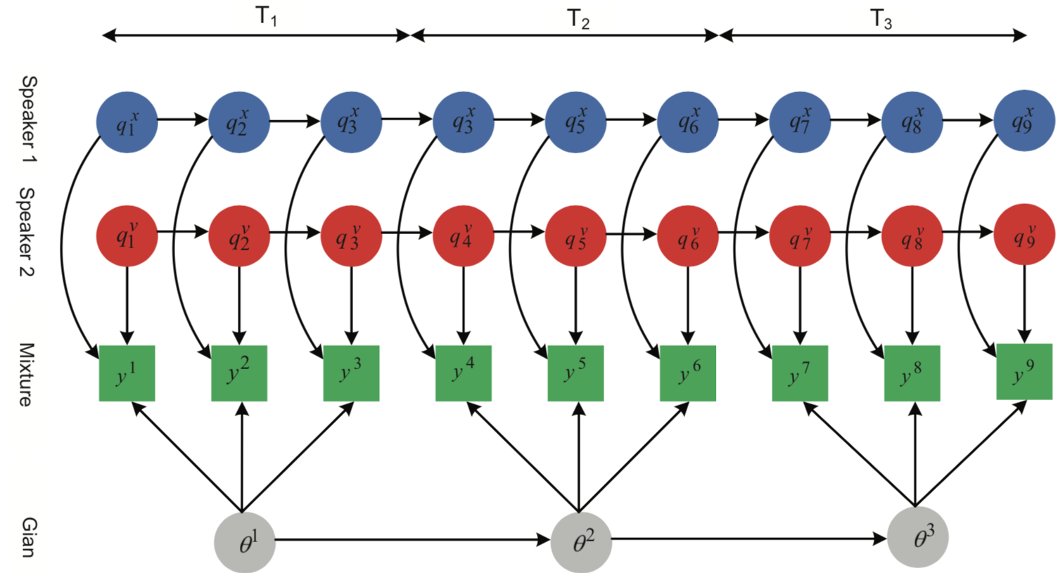
Figure 1: A graphical representation of GFHMM consisting of three hidden states modeling the log spectral vectors of two speakers (${\mathbf{q}}^{x}$ and ${\mathbf{q}}^{v}$) and gain ratio ($\theta$) as well as an observed state modeling the mixture ($y$). Speakers’ hidden states are decoded at frame level ($r=10$ msec) and gain state is decoded at mega frame rate ($T_{i}=2$ sec).

We make inference using GFHMM, a graphical model illustrated in Fig. 1. GFHMM consists of three independent hidden layers, two HMMs correspond to speakers’ spectral patterns, and one hidden node corresponds to target-to-interference ratio, $\theta$ . Our model exploits the fact that the speakers’ loudness ($g_{x}$ and $g_{v}$) is almost constant within short time intervals, namely one to two seconds. Thus, while spectral pattern decoding is updated at each frame (10 msec), $\theta$ decoding is updated at mega frame level (1$\leq T\leq 2$sec.). Probabilistically, we wish to maximize the joint probability of the observed signal and hidden states, given the model parameters and $\theta$. Given the observation log spectral vectors ${\mathbf{y}}\triangleq({\mathbf{y}}^{1},\dotsc,{\mathbf{y}}^{r},\dotsc,{\mathbf{y}}^{R})$ and the parameter sets $\lambda_{x}(\pi^{x},a^{x},b^{x})$, $\lambda_{v}(\pi^{v},a^{v},b^{v})$, and $\theta$, we aim at finding the best state sequences $\tilde{{\mathbf{q}}}^{x}=(\tilde{q}^{x}_{1},\tilde{q}^{x}_{2},\dotsc\,\tilde{q}^{x}_{r},\dotsc\,\tilde{q}^{x}_{R})$ and $\tilde{{\mathbf{q}}}^{v}=(\tilde{q}^{v}_{1},\tilde{q}^{v}_{2},\dotsc\,\tilde{q}^{v}_{r},\dotsc\,\tilde{q}^{v}_{R})$ which maximize

$${\tilde{{\mathbf{q}}}^{x},\tilde{{\mathbf{q}}}^{v}}=\underset{{\mathbf{q}}^{x},{\mathbf{q}}^{v}}{\operatorname{argmax}}\,\,p({\mathbf{q}}^{x},{\mathbf{q}}^{v},{\mathbf{y}}|\lambda_{x},\lambda_{v},\theta).$$ (10)

For now, we assume that $\theta$ is known in advance. In the next subsection, we propose an approach for estimating $\theta$. We solve the maximization problem in (10) using the parallel Viterbi algorithm, which is, in fact, a two-dimensional form of the original Viterbi algorithm [40, page 729]. To do this, we first define the variable

$$\delta_{r}(i,\ell,\theta) = \underset{q^{v}_{1},q^{v}_{2},\dotsc,q^{v}_{r}}{\underset{q^{x}_{1},q^{x}_{2},\dotsc,q^{x}_{r}}{\max}}\,\,p(q^{x}_{1},q^{x}_{2},\dotsc,q^{x}_{r}=i,q^{v}_{1},q^{v}_{2},\dotsc,q^{v}_{r}=\ell$$

$$,{\mathbf{y}}^{1},{\mathbf{y}}^{2},\dotsc,{\mathbf{y}}^{r}|\lambda_{x},\lambda_{v},\theta)$$

which is the probability corresponding to the two best paths from the first to the $r^{\text{th}}$ observation. For the $(r+1)^{\text{th}}$ observation, we have

$$\delta_{r+1}(j,k,\theta)=[\underset{i,\ell}{\max}\ \delta_{r}(i,\ell,\theta)\,a^{x}_{ij}\,a^{v}_{\ell k}]b_{j,k}({\mathbf{y}}^{r+1}|\theta)$$ (11)

where

$$b_{j,k}({\mathbf{y}}^{r+1}|\theta)=p({\mathbf{y}}^{r+1}|q^{x}_{r+1}=j,q^{v}_{r+1}=k|\theta).$$ (12)

Using these definitions, we now present the parallel Viterbi algorithm. It should be noted that the parallel Viterbi algorithm, like the Viterbi algorithm, can be implemented by applying either probabilities directly or the log of probabilities. We use the latter since it reduces computations (replacing multiplication by summation) and prevents numerical instability, which should be carefully treated since we deal with probabilities of the order of $10^{-200}$. The parallel Viterbi algorithm in the log domain is carried out in five steps, as follows:

• Preprocessing

  • $\hat{\pi}^{x}_{j}=\log\pi^{x}_{j}$, and $\hat{\pi}^{v}_{k}=\log\pi^{v}_{k}$, $\quad 1\leq j,k\leq K$

  • $\hat{b}_{j,k}({\mathbf{y}}^{r}|\theta)=\log b_{j,k}({\mathbf{y}}^{r}|\theta)$,$\quad 1\leq j,k\leq K$,   $1\leq r\leq R$

  • $\hat{a}^{x}_{ij}=\log a^{x}_{ij}$, and $\hat{a}^{v}_{\ell k}=\log a^{v}_{\ell k}\quad 1\leq i,j,\ell,k\leq K$

• Initialization

  • $\hat{\delta}_{1}(j,k,\theta)=\log\delta_{1}(j,k,\theta)=\hat{\pi}^{x}_{j}+\hat{\pi}^{v}_{k}+\hat{b}_{j,k}({\mathbf{y}}^{1}|\theta)\quad 1\leq j,k\leq K$

  • $\psi_{r}(j,k)=0\quad 1\leq j,k\leq K$ ,   $1\leq r\leq R$

• Recursion

  • $\hat{\delta}_{r}(j,k,\theta)=\log\delta_{r}(j,k,\theta)=\underset{1\leq i,\ell\leq K}{\max}[\hat{\delta}_{r-1}(i,\ell,\theta)+\hat{a}^{x}_{ij}+\hat{a}^{v}_{\ell k}]+\hat{b}_{j,k}({\mathbf{y}}^{r}|\theta)\quad 1\leq j,k\leq K$,   $2\leq r\leq R$

  • $\psi_{r}(j,k)=\underset{1\leq i,\ell\leq K}{\operatorname{argmax}}[\hat{\delta}_{r-1}(i,\ell,\theta)+\hat{a}^{x}_{ij}+\hat{a}^{v}_{\ell k}]\quad 1\leq j,k\leq K$,   $2\leq r\leq R$

• Termination

  • $P(\theta)=\underset{1\leq i,\ell\leq K}{\max}\hat{\delta}_{R}(i,\ell,\theta)$

  • ($\tilde{q}^{x}_{R},\tilde{q}^{v}_{R})=\underset{1\leq i,\ell\leq K}{\operatorname{argmax}}\hat{\delta}_{R}(i,\ell,\theta)$

• Path backtracking

  • $(\tilde{q}^{x}_{r},\tilde{q}^{v}_{r})=\psi_{r+1}(\tilde{q}^{x}_{r+1},\tilde{q}^{v}_{r+1})\quad r=R-1,R-2,\dotsc,1$

In this way, we decode the two best state sequences which maximize the joint state sequence probability and observation. The selected state sequences are then used to build filters whereby the target and interference are estimated. This subject will be discussed in Sec. IV.

III-B Observation Signal Probability

In the previous subsection, we described the parallel Viterbi algorithm for decoding the two best state sequences. In this algorithm, computing $b_{j,k}({\mathbf{y}}^{r}|\theta)=p({\mathbf{y}}^{r}|q^{x}_{r}=j,q^{v}_{r}=k,\theta)$ plays an important role. Here, we explain how to calculate this PDF in terms of the PDF of the target and the PDF of the interference, and the gain factors. In [23, IV.A], we obtained an approximation to $p(y^{r}(d)|q^{x}_{r}=j,q^{v}_{r}=k,\theta)$ in terms of the PDFs of $x^{r}(d)$ and $v^{r}(d)$ when $g_{x}=g_{v}=0$. Adding $\log_{10}g_{x}=g(\theta)$ and $\log_{10}g_{v}=g(-\theta)$ to ${\mathbf{x}}^{r}$ and ${\mathbf{v}}^{r}$ shifts only the means of the PDFs of ${\mathbf{x}}^{r}$ and ${\mathbf{v}}^{r}$ by $g(\theta)$ and $g(-\theta)$, respectively, and thus the PDF of ${\mathbf{y}}$ is given by

$$p({\mathbf{y}}^{r}|q^{x}_{r}=j,q^{v}_{r}=k,\theta)\approx\prod_{d=0}^{D-1}\frac{1}{\sqrt{2\pi\sigma^{2}_{\max}(d)}}\times$$

$$\exp\Bigl{(}-\frac{\Bigl{(}y^{r}(d)-\max\bigl{(}\mu^{j}_{x}(d)+g(\theta),\mu^{k}_{v}(d)+g(-\theta)\bigr{)}\Bigr{)}^{2}}{2\sigma^{2}_{\max}(d)}\Bigr{)},$$

where $\sigma^{2}_{\max}(d)$ is the variance of the source whose mean is greater than the other—for instance, if $\mu^{j}_{x}(d)\geq\mu^{k}_{v}(d)$, then $\sigma_{\max}(d)=\sigma^{j}_{x}(d)$. Hence, $\hat{b}_{j,k}({\mathbf{y}}^{r}|\theta)$ in the log-based parallel Viterbi algorithm is simply obtained by

$$\hat{b}_{j,k}({\mathbf{y}}^{r}|\theta)=$$

$$- \sum_{d=0}^{D-1}\frac{1}{2}\Bigl{(}\frac{y^{r}(d)-\max\bigl{(}\mu^{j}_{x}(d)+g(\theta),\mu^{k}_{v}(d)+g(-\theta)\bigr{)}}{\sigma_{\max}(d)}\Bigr{)}^{2}$$

$$- \log\sigma_{\max}(d)-\frac{1}{2}\log 2\pi,$$

III-C Estimating $\theta$ using Quadratic Optimization

The formulas derived for the parallel Viterbi algorithm assume that the $\theta$ is given in advance. Here, we propose an approach to estimate the $\theta$. We assume that $\theta$ lies in the interval $\Theta=[\theta_{\min};\theta_{\max}]$ over which the separation of two signals is feasible. This means that for those $\theta$s outside the range for $\Theta$, the stronger source almost completely masks the weaker source, i.e. $g_{x}\gg g_{v}\rightarrow Y(t)\approx g_{x}X(t)$ or vice versa. In this paper, we set $\theta_{\min}=-15$ dB and $\theta_{\max}=15$ dB.

For an given arbitrary pair of ${\mathbf{q}}^{x}$ and ${\mathbf{q}}^{v}$, the joint probability $p({\mathbf{q}}^{x},{\mathbf{q}}^{v},{\mathbf{y}}|\lambda_{x},\lambda_{v},\theta)$, (10), becomes a likelihood function of $\theta$, denoted by $\mathcal{L}(\theta|{\mathbf{q}}^{x},{\mathbf{q}}^{v})$. One naive approach to decode the best two pathes and $\theta$ is to compute the likelihood function for all possible pairs in term of $\theta$ and select the pair and $\theta$ which maximize the likelihood. When implementing this procedure, we observed that $\mathcal{L}(\theta|\overset{1}{{\mathbf{q}}^{x}},\overset{1}{{\mathbf{q}}^{v}})\geq\mathcal{L}(\theta|\overset{2}{{\mathbf{q}}^{x}},\overset{2}{{\mathbf{q}}^{v}})\geq\mathcal{L}(\theta|\overset{3}{{\mathbf{q}}^{x}},\overset{3}{{\mathbf{q}}^{v}})\geq\ldots\mathcal{L}(\theta|\overset{m}{{\mathbf{q}}^{x}},\overset{m}{{\mathbf{q}}^{v}})\geq\ldots\geq\mathcal{L}(\theta|\overset{K^{2}}{{\mathbf{q}}^{x}},\overset{K^{2}}{{\mathbf{q}}^{v}})$ for any value of $\theta$, where $m$ in $\mathcal{L}(\theta|\overset{m}{{\mathbf{q}}^{x}},\overset{m}{{\mathbf{q}}^{v}})$ represents the rank of likelihood of a pair of states $({\mathbf{q}}^{x},{\mathbf{q}}^{v})$ as decoded by the parallel Viterbi algorithm with some initial value $\theta_{0}$. Moreover, we observed that $\mathcal{L}(\theta|\overset{m}{{\mathbf{q}}^{x}},\overset{m}{{\mathbf{q}}^{v}})$ approximately resembles a quadratic form. Fig. 2 provides an illustration of the likelihood of the 20 top pairs $(\overset{m}{{\mathbf{q}}^{x}},\overset{m}{{\mathbf{q}}^{v}})$ decoded by the Viterbi algorithm as a function of $\theta$. As shown the likelihood associated to the best path decoded by the Viterbi algorithm is distinctly greater than the second top for all values of $\theta$, and so forth.

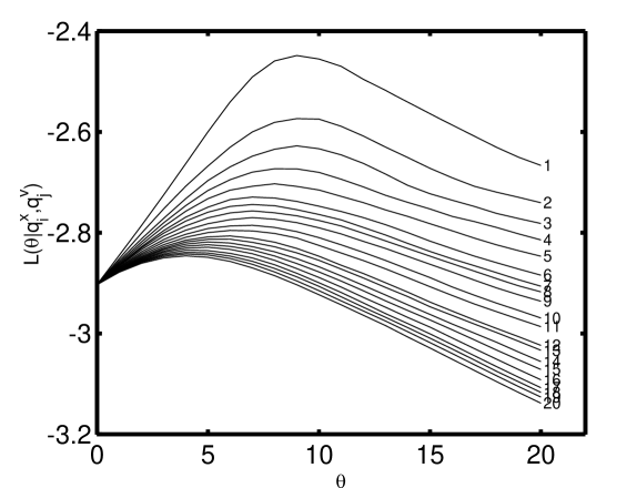
Figure 2: The likelihood of 20 top pairs of $({\mathbf{q}}^{x},{\mathbf{q}}^{v})$ as a function of $\theta$ (dB).

Since $\mathcal{L}(\theta|{\mathbf{q}}^{x},{\mathbf{q}}^{v})$ is well-approximated by a quadratic function, $\theta$ can be readily estimated using quadratic optimization rather than performing an exhaustive search. Fig. 3 shows a block diagram of the proposed method for decoding the best paths $\{{\mathbf{q}}_{s}^{x},{\mathbf{q}}_{s}^{v}\}_{s=1}^{S}$ and $\tilde{\theta}$. Using the decoded path and the quadratic optimization approach, the value of $\theta$ is updated until the maximum of $\mathcal{L}(\theta|{\mathbf{q}}^{x},{\mathbf{q}}^{v})$ is reached. In the experiments, we show that the maximum is reached within two or three iterations. The procedure for estimating the maximum of a quadratic function using iterative methods can be found in [41, page 499] and [42].

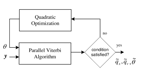
Figure 3: A high level block diagram of the gain adapted FHMM-based SCSS approach.

IV Recovering Target and Interference using the Decoded Parameters

In the previous section, we proposed how to obtain the best state sequences for trained HMMs, i.e., $\tilde{{\mathbf{q}}}^{x}$ and $\tilde{{\mathbf{q}}}^{v}$, and the $\theta$ which best model the mixture in a maximum likelihood sense. Here, we apply the decoded parameters to build two filters, known as binary masks, which when applied to the mixture yields estimates of the target and interference signals. Using the mean vectors of the decoded states, the binary mask to estimate the target is given by

$$H^{r}_{x_{HMM}}(d)=\begin{cases}\,1,\,&\mu^{\tilde{q}^{x}_{r}}_{x}(d)+\hat{g}(\tilde{\theta})\geq\mu^{\tilde{q}^{v}_{r}}_{v}(d)+\hat{g}(-\tilde{\theta})\\ 0\,,&\mu^{\tilde{q}^{x}_{r}}_{x}(d)+\hat{g}(\tilde{\theta})<\mu^{\tilde{q}^{v}_{r}}_{v}(d)+\hat{g}(-\tilde{\theta})\end{cases}$$ (13)

$d=0,\dotsc,D-1$, whereas the binary mask for the interference is given by $H^{r}_{v_{HMM}}(d)=1-H^{r}_{x_{HMM}}(d)$. In (13), $\mu^{\tilde{q}^{x}_{r}}_{x}(d)$ and $\mu^{\tilde{q}^{v}_{r}}_{v}(d)$ represent the $d$th components of the mean vectors of the decoded states of the target and interference HMMs, respectively, for the $r$th frame. The target binary mask is multiplied with the $D$-point DFT of the $r$th frame of the observation and then the $D$-point inverse DFT is applied to the resulting vector to give an estimate of the target in the time domain:

$$\{\widehat{X}(t)\}_{t=(r-1)M}^{(r-1)M+N-1}=$$

$$\mathcal{F}^{-1}_{D}\biggl{(}H^{r}_{x_{HMM}}(d)\mathcal{F}_{D}\Bigl{(}\{Y(t)\}_{t=(r-1)M}^{(r-1)M+N-1}\Bigr{)}\biggr{)},$$

$r=1,\dotsc,R$ , where $\mathcal{F}_{D}(\cdot)$ and $\mathcal{F}^{-1}_{D}(\cdot)$ represent the $D$-point forward and inverse Fourier transform, respectively, and $\{\widehat{X}(t)\}_{t=(r-1)M}^{(r-1)M+N-1}$ is the estimated target in the time domain. Finally, the time-domain vectors are multiplied by a Hann window and the overlap-add method [43] is used to recover the target signal. An estimated time-domain interference signal is obtained in a similar fashion. The entire procedure for separating signals using GFHMM approach is shown in Figure 4.

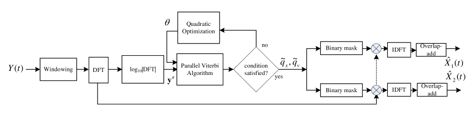
Figure 4: A schematic of GFHMM-based SCSS.

V Experiments

V-A Experimental Setup

Speech files considered for the experiments were selected from the database presented in [44]. The database consists of speech files of 34 speakers, each of which uttered 500 sentences. 12 speakers were selected to form the mixtures of female-female, male-male, and female-male pairs. Table I lists the selected speakers and the indexes of selected speech files for evaluation. The selected speech files were not included in the training phase. After mixing speech files, 10 female-female, 10 male-male, and 10 female-male mixtures (observations) were obtained. The speech files were mixed at the TIRs of 0, 3, 6, 9, 12, and 15 dB such that 180 different observations are generated for the experiments. One of the speech signals in each mixture was treated as the target while the other one as the interference. Throughout the experiments, a Hamming window of length 32 msec with the frame shift equal to 10 msec was used to segment the speech files. Also, a Hann window was used in the overlap-add method for synthesizing the separated speech signals. The sampling rate was decreased to 8 kHz from the original 25 kHz in the database presented in [44].

For each speaker, 100 sentences were used for HMM and VQ training (for gain adapted VQ SCSS see Appendix I). The windowed training speech files were transformed into the log frequency domain using a 256-point discrete Fourier transform ($D=256$), resulting in log spectral vectors of dimension 129. For VQ modeling, the LBG VQ algorithm [45] with binary splitting initialization was used to construct a 64-entry codebook ($K=64$) for each speaker. For HMM modeling, we used the Baum-Welch method [46] to estimate the HMM parameters. The number of states was set to 64 ($K=64$). The initial estimates of the HMM parameters are obtained from the VQ training. Accordingly, the initial mean vector of each HMM state was set to a codevector and the variance of each cluster in VQ was considered as the covariance matrix of each HMM state (we assume the covariance matrix is diagonal). The ratio between the number of vectors in each cluster to the total number of training vectors was used as the initial state probability for the corresponding state. The Baum-Welch algorithm was terminated when the difference between the current and previous log likelihoods was less than 0.00001, or the maximum number of iterations (15) was reached.

TABLE I: Speech files selected for experiments from the database introduced in [44].

Type I (female-male):
spk1	1	18	3	25	6	1	4	24	3	18
sen1	159	138	34	130	149	40	174	162	42	190
spk2	4	2	24	5	7	18	5	6	11	2
sen2	140	182	115	143	167	133	37	72	76	76
Type II (male-male):
spk1	1	2	6	17	5	2	1	3	5	2
sen1	160	40	139	174	66	144	149	35	100	28
spk2	3	5	17	1	6	3	6	17	17	6
sen2	176	196	38	159	21	76	66	160	38	22
Type III (female-female):
spk1	4	24	7	4	18	24	25	4	18	4
sen1	137	88	63	51	153	125	124	52	25	128
spk2	18	25	11	24	25	7	11	11	7	25
sen2	57	175	72	126	94	129	75	42	63	40

V-B Methods for Comparison

The performance of GFHMM was compared with the gain adapted VQ (GVQ) (See Appendix I), FHMM [19], and VQ [26] based SCSS. The comparison with the VQ-based SCSS was done to assess the performance improvement when memory (HMM-based approach) is incorporated into the separation system.

Since GFHMM involves an iterative stage (quadratic optimization) and since convergence speed is an important factor for practical situations, the number of iterations required for the convergence of GFHMM was also reported.

Furthermore, to evaluate the impact of errors in the estimation of $\tilde{\theta}$ obtained by the quadratic optimization on separation performance, GFHMM was also run assuming the knowledge of the actual $\theta$ in advance (i.e., the quadratic optimization was removed and the actual $\theta$ was used).

V-C Results

In order to evaluate the separation performance of the proposed techniques, the signal-to-noise ratio (SNR) between the estimated, i.e., $\hat{Z}(t)$, and original, i.e. $Z(t)$, speech files defined by

$$\text{SNR}=10\log_{10}\bigg{[}\frac{\sum_{t}\bigl{(}Z(t)\bigr{)}^{2}}{\sum_{t}\bigl{(}Z(t)-\hat{Z}(t)\bigr{)}^{2}}\bigg{]}\qquad t=0,1,\dotsc,T-1$$ (14)

was used where $Z(t)\in\{X(t),V(t)\}$. SNR results are shown in Fig. 5-Fig. 10. Fig. 5, Fig. 7, and Fig. 9 show the SNR versus $\theta$ averaged over 10 separated target speech files for female-female, male-male, and female-male mixtures, respectively, for: GFHMM ($\circ$ line),GFHMM (with actual $\theta$) ($\Box$ line), GVQ ($\lhd$ line), GVQ (with actual $\theta$) ($\diamondsuit$ line ), HMM ($\rhd$ line), and VQ ($\triangle$ line). Also, Fig. 6, Fig. 8, and Fig. 10 show the same respective results, but for the separated interference signals. From the figures, several observations can be made which hold true for all three types of mixtures.

The first observation is that as $\theta$ increases the SNRs for the target signals increase as well and, on the contrary, the SNRs decrease for the interference signals. This behavior of the SNR curves versus $\theta$ is quite expected since a signal with higher power can be better separated from the weaker one. Comparing the GFHMM technique with the actual and estimated $\theta$ ($\circ$ lines with $\Box$ lines), we see that the SNR results are almost the same. In fact, even slight improvements are seen for the scaled HMM with $\theta$ estimated using quadratic optimization. The same observation is also valid for the GVQ with actual and estimated $\theta$ ($\lhd$ lines with ($\diamondsuit$ lines). It should be noted that an ideal $\theta$ for the separation process might differ from the actual $\theta$ since the actual $\theta$ is the best choice only if the actual, rather than the model-supplied, log spectral vectors are used for separation.

Comparing SNR results of GFHMM and GVQ techniques ($\circ$ lines with ($\lhd$ lines), we observe that GFHMM outperforms the GVQ for both target and interference signals in all three type of mixtures. Although the former outperforms the latter, the improvement is not very large considering the sheer complexity of HMM when compared with VQ which is remarkably simpler and faster than HMM. The search complexity of the parallel Viterbi algorithm is $O(RK^{3})$ [47] whereas the search complexity of the VQ technique is $O(RK^{2})$.

We also compare SNR results obtained from GFHMM with HMM, and GVQ with VQ ($\circ$ and $\lhd$ lines with $\rhd$ and $\triangle$ lines, respectively). The results show that the gain adapted versions of HMM and VQ significantly outperform the non-gain adapted ones. The improvement is quite palpable for $\theta\text{s}>6$  dB. The results confirm that the model-based non-gain adapted SCSS techniques fail to separate the speech signals when the test samples have energies substantially different from those used in the training data set. For all the above techniques, the separation of interference signals at $\theta>6$ dB is a difficult task as the separated interference signal has very poor quality, showing that solving this problem remains a challenge for future studies.

In Fig. 11, Fig. 12, and Fig. 13, $\tilde{\theta}$ is compared with the actual $\theta$ in the upper panels, and in the lower panels the number of iterations to reach convergence is reported for GFHMM and GVQ techniques. For both cases, results are averaged over 10 separated speech files. From the upper panels, one can see that estimated $\tilde{\theta}$-s are very close to the actual $\theta$-s. Form the lower panels, it is seen that the GFHMM converges with less than 3 iterations on average. Also, GVQ converges faster than GFHMM. The results given in Fig. 11, Fig. 12, and Fig. 13 show that the proposed quadratic optimization approach not only well-approximate $\theta$, but also converges very fast.

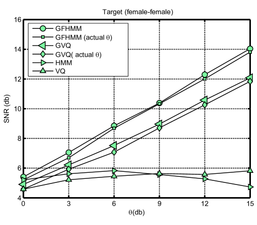
Figure 5: SNR versus $\theta$ averaged over 10 separated target speech files from female-female mixtures using GFHMM ($\circ$ line), GFHMM (with actual $\theta$) ($\Box$ line), GVQ ($\lhd$ line), GVQ (with actual $\theta$) ($\diamondsuit$ line), HMM ($\rhd$ line), and VQ ($\triangle$ line).

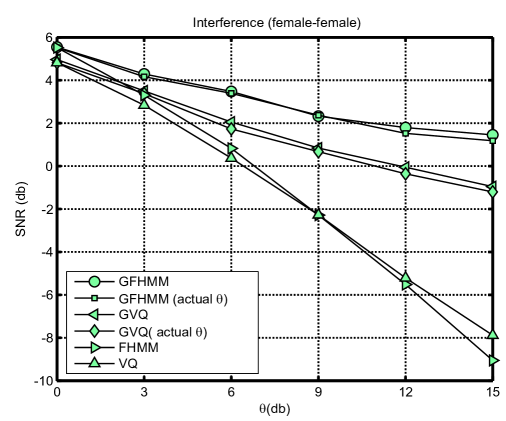
Figure 6: SNR versus $\theta$ averaged over 10 separated interference speech files from female-female mixtures using GFHMM ($\circ$ line), GFHMM (with actual $\theta$) ($\Box$ line), GVQ ($\lhd$ line), GVQ (with actual $\theta$) ($\diamondsuit$ line), HMM ($\rhd$ line), and VQ ($\triangle$ line).

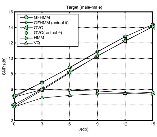
Figure 7: SNR versus $\theta$ averaged over 10 separated target speech files from male-male mixtures using GFHMM ($\circ$ line), GFHMM (with actual $\theta$) ($\Box$ line), GVQ ($\lhd$ line), GVQ (with actual $\theta$) ($\diamondsuit$ line), HMM ($\rhd$ line), and VQ ($\triangle$ line).

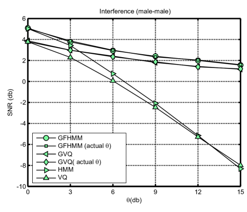
Figure 8: SNR versus $\theta$ averaged over 10 separated interference speech files from male-male mixtures using GFHMM ($\circ$ line), GFHMM (with actual $\theta$) ($\Box$ line), GVQ ($\lhd$ line), GVQ (with actual $\theta$) ($\diamondsuit$ line), HMM ($\rhd$ line), and VQ ($\triangle$ line).

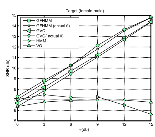
Figure 9: SNR versus $\theta$ averaged over 10 separated target speech files from female-male mixtures using GFHMM ($\circ$ line), GFHMM (with actual $\theta$) ($\Box$ line), GVQ ($\lhd$ line), GVQ (with actual $\theta$) ($\diamondsuit$ line), HMM ($\rhd$ line), and VQ ($\triangle$ line).

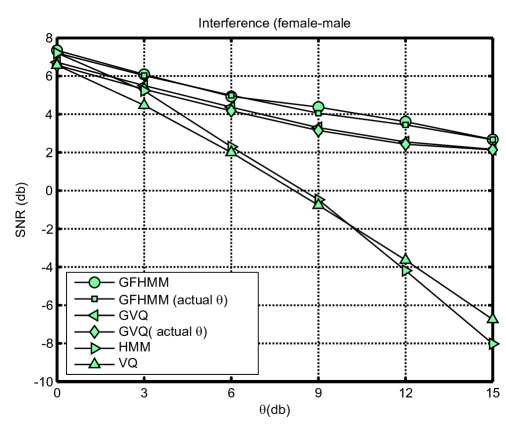
Figure 10: SNR versus $\theta$ averaged over 10 separated interference speech files from female-male mixtures using GFHMM ($\circ$ line), GFHMM (with actual $\theta$) ($\Box$ line), GVQ ($\lhd$ line), GVQ (with actual $\theta$) ($\diamondsuit$ line), HMM ($\rhd$ line), and VQ ($\triangle$ line).

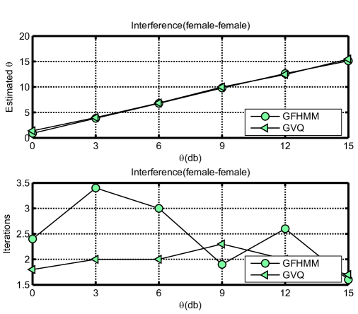
Figure 11: Estimated $\theta$ versus actual $\theta$ (upper panel) and number of iterations (lower panel) averaged over 20 separated target and interference speech files from female-female mixtures using GFHMM ($\circ$ line) and GVQ ($\lhd$ line).

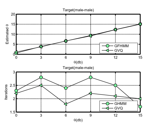
Figure 12: Estimated $\theta$ versus actual $\theta$ (upper panel) and number of iterations (lower panel) averaged over 20 separated target and interference speech files from male-male mixtures using GFHMM ($\circ$ line) and GVQ ($\lhd$ line).

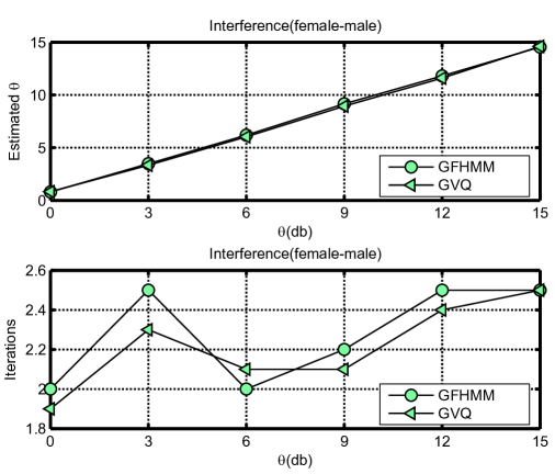
Figure 13: Estimated $\theta$ versus actual $\theta$ (upper panel ) and number of iterations (lower panel) averaged over 20 separated target and interference speech files from female-male mixtures using GFHMM ($\circ$ line) and GVQ ($\lhd$ line).

VI Conclusions

In probabilistic model based single channel speech separation, the objective is to estimate the model parameters that maximize the joint probability of the observed mixture and the hidden variables. The exact computing of this probability is, however, intractable. Factorial hidden Markov models offer tractable approximation to the probabilistic model by decoupling states of the target and interference signals. Nonetheless, even using FHMM as a probabilistic framework, the inference becomes computationally prohibitive when more than two hidden layers are used. Accordingly, the use of FHMM for SCSS is practically limited to two-independent hidden layers (one for the target signal and one for the interference signal). Previous FHMM models assume that speakers’ loudness is the same in training and test data. In this paper we address this shortcoming by introducing a gain-adapted FHMM. In our model, we explicitly introduce the gain factor for the target and interference signals. In GFHMM, the number of hidden layers of the FHMM remains two, and the gain factors are estimated using quadratic optimization. This makes the computational complexity of GFHMM similar to FHMM. Our experiments show that the introduction of the explicit gain factor to the FHMM model improves the results of separation. The improvements becomes very significant when the gain mismatch between training and test signals increases. In addition to speech separation, GFHMM can be potentially applied to other speech processing problems such as speech enhancement and robust speech recognition where gain mismatch may reduce the performance.

[gain adapted VQ-Based SCSS] The gain adapted VQ (GVQ) [38] can be considered as memoryless version of GFHMM . In GVQ, the feature space (log spectral vectors) is partitioned into $K$ clusters using the LBG algorithm and the centroids of the regions are codevectors that represent the clusters. The goal is to find the codevectors and $\theta$ which best model the observation. The selected codevectors and $\theta$ are then used to build filters to recover the target and interference. Let $\mathcal{C}_{x}=\{{\mathbf{c}}_{x}^{i},\,i=1,\dotsc,K\},\,{\mathbf{c}}_{x}^{i}=\{c_{x}^{i}(d)\}_{d=0}^{D-1}$, be a $K$-entry codebook of log spectral vectors of the target signal. Let $\mathcal{C}_{v}=\{{\mathbf{c}}_{v}^{j},\,j=1,\dotsc,K\},\,{\mathbf{c}}_{v}^{j}=\{c_{v}^{j}(d)\}_{d=0}^{D-1}$, be a $K$-entry codebook of log spectral vectors of the interference signal.The algorithm can be explained as follows. Let ${\mathbf{s}}^{x}\triangleq(s^{x}_{1},s^{x}_{2},\dotsc,s^{x}_{r},\dotsc,s^{x}_{R})$, $s^{x}_{r}\in\{1,\dotsc,K\}$, and ${\mathbf{s}}^{v}\triangleq(s^{v}_{1},s^{v}_{2},\dotsc,s^{v}_{r},\dotsc,s^{v}_{R})$, $s^{v}_{r}\in\{1,\dotsc,K\}$, be the codevector index sequences for the target and interference codebooks $\mathcal{C}_{x}$ and $\mathcal{C}_{v}$, respectively. For a given $\theta$ and each frame, the indices of the pair of codevectors that minimize the following cost function are found.

$$e^{r}(s^{x}_{r}=i^{*},s^{v}_{r}=j^{*},\theta)=\underset{1\leq i,j\leq K}{\text{min}}\,\,$$

$$\sum_{d=0}^{D-1}\Bigl{(}y^{r}(d)-\max\bigl{(}c^{i}_{x}(d)+g_{x}(\theta),c^{j}_{v}(d)+g_{v}(-\theta)\bigr{)}\Bigr{)}^{2}.$$

which implies that, for a given $\theta$, the codevectors $c^{i^{*}}_{x}$ and $c^{j^{*}}_{v}$ that minimize the Euclidean distance between ${\mathbf{y}}^{r}$ and the right hand sight of (9) when the original vectors ${\mathbf{x}}^{r}$ and ${\mathbf{v}}^{r}$ are replaced with the codevectors from $\mathcal{C}_{x}$ and $\mathcal{C}_{v}$. The cost functions are summed up over all frames to get

$$Q(\theta)=-\sum_{r=1}^{R}e^{r}(s^{x}_{r}=i^{*},s^{v}_{r}=j^{*},\theta)$$ (15)

which is GVQ counterpart to $P(\theta)$ in GFHMM . A similar procedure to the one shown in Fig. 3 is then carried out for the GVQ in which $P(\theta)$ is replaced with $Q(\theta)$ and the Viterbi decoding with (VI). Finally similar to GFHMM, for recovering the source signals we build two binary masks using the decoded codevectors as follows

$$H^{r}_{x_{VQ}}(d)=\begin{cases}\,1,\,&c^{\tilde{s}^{x}_{r}}_{x}(d)+\hat{g}(\tilde{\theta})\geq c^{\tilde{s}^{v}_{r}}_{v}(d)+\hat{g}(-\tilde{\theta})\\ 0\,,&c^{\tilde{s}^{x}_{r}}_{x}(d)+\hat{g}(\tilde{\theta})<\mu^{\tilde{s}^{v}_{r}}_{v}(d)+\hat{g}(-\tilde{\theta})\end{cases}$$ (16)

$d=0,\dotsc,D-1$, and the binary mask for the interference signal is $H^{r}_{v_{VQ}}(d)=1-H^{r}_{x_{VQ}}(d)$ where $c^{\tilde{s}^{x}_{r}}_{x}(d)$ and $c^{\tilde{s}^{v}_{r}}_{v}(d)$ present $d$th components of the selected codevectors from the target and interference codebooks, respectively, for the $r$th frame.

References

- [1] E. C. Cherry, On human communication: A review, survey, and a criticism, Cambridge, MA: MIT Press, 1957.
- [2] A. S. Bregman, Computatinal Auditory Scene Analysis, MIT Press, Cambridge MA, 1994.
- [3] Pierre Divenyi, Ed., Speech Separation by Humans and Machines, Springer, 1 edition, 2004.
- [4] D. Ellis, “Model-based scene analysis,” in Computational Auditory Scene Analysis: Principles, Algorithms, and Applications, D. Wang and G. Brown, Eds. Wiley/IEEE Press, 2006.
- [5] D.L. Wang and G. J. Brown, Eds., Computational Auditory Scene Analysis: Principles, Algorithms, and Applications, Wiley-IEEE Press, 2006.
- [6] P. Li, Y. Guan, B. Xu, and W. Liu, “Monaural speech separation based on computational auditory scene analysis and objective quality assessment of speech,” IEEE Trans. on Speech and Audio Processing, vol. 14, no. 6, pp. 2014–2023, Nov. 2006.
- [7] G. J. Brown and M. Cooke, “Auditory scene analysis,” Computer Speech and Language, vol. 8, no. 4, pp. 297–336, 1994.
- [8] T. Virtanen and A. Klapuri, “Separation of harmonic sound sources using sinusoidal modeling,” in Proc. ICASSP–2000, June 2000, pp. 765–768.
- [9] G.J. Brown and D.L. Wang, Speech Enhancement, chapter Separation of speech by computational auditory scene analysis, pp. 371–402, Springer, New York, 2005.
- [10] J. F. Cardoso, “Blind signal separation: Statistical principles,” Proceedings of the IEEE, vol. 86, no. 10, pp. 2009–2025, 1998.
- [11] C. Jutten and J. Herault, “Blind separation of sources, Part I: An adaptive algorithm based on neuromimetic architecture,” Signal Processing, vol. 24, pp. 1–10, 1991.
- [12] P. Common, “Independent component analysis, a new concept?,” Signal Processing, vol. 36, pp. 287–314, 1994.
- [13] A. J. Bell and T. J. Sejnowski, “An information-maximization approach to blind separation and blind deconvolution,” Neural Computation, vol. 7, pp. 1129–1159, 1995.
- [14] S. I. Amari and J. F. Cardoso, “Blind source separation–semiparametric statistical approach,” IEEE Trans. Signal Processing, vol. 45, no. 11, pp. 2692–2700, 1997.
- [15] D. Model and M. Zibulevsky, “Signal reconstruction in sensor arrays using sparse representations,” Signal Processing, vol. 86, no. 3, pp. 624–638, 2006.
- [16] M. H. Radfar, R. M. Dansereau, and A. Sayadiyan, “A maximum likelihood estimation of vocal-tract-related filter characteristics for single channel speech separation,” EURASIP Journal on Audio, Speech, and Music Processing, vol. 2007, pp. Article ID 84186, 15 pages, 2007, doi:10.1155/2007/84186.
- [17] M. H. Radfar, R. M. Dansereau, and A. Sayadiyan, “Monaural speech segregation based on fusion of source-driven with model-driven techniques,” Speech Communication, vol. 49, no. 6, pp. 464–476, June 2007.
- [18] G. Hu and D. L. Wang, “Monaural speech segregation based on pitch tracking and amplitude modulation,” IEEE Trans. Neural Networks, vol. 15, no. 5, pp. 1135–1150, Sept. 2004.
- [19] S. Roweis, “One microphone source separation,” in Proc. Neural Inf. Process. Syst., 2000, pp. 793–799.
- [20] M. J. Reyes-Gomez, D. Ellis, and N. Jojic, “Multiband audio modeling for single channel acoustic source separation,” in Proc. ICASSP–04, May 2004, vol. 5, pp. 641–644.
- [21] R.J. Weiss and D.P.W. Ellis, “Speech separation using speaker-adapted eigenvoice speech models,” Computer Speech & Language, vol. 24, no. 1, pp. 16–29, 2010.
- [22] T. Kristjansson, H. Attias, and J. Hershey, “Single microphone source separation using high resolution signal reconstruction,” in Proc. ICASSP–04, May 2004, pp. 817–820.
- [23] M. H. Radfar and R. M. Dansereau, “Single channel speech separation using soft mask filtering,” IEEE Transactions on Audio, Speech and Language Processing, vol. 15, no. 8, pp. 2299–2310., Nov. 2007.
- [24] A. M. Reddy and B. Raj, “Soft mask methods for single-channel speaker separation,” Audio, Speech and Language Processing, IEEE Transactions on, vol. 15, no. 6, pp. 1766–1776, Aug. 2007.
- [25] S. T. Rowies, “Factorial models and refiltering for speech separation and denoising,” in EUROSPEECH–03, May 2003, vol. 7, pp. 1009–1012.
- [26] M. H. Radfar, R. M. Dansereau, and A. Sayadiyan, “Performance evaluation of three features for model-based single channel speech separation problem,” in Interspeech 2006, Intern. Conf. on Spoken Language Processing (ICSLP’2006 Pittsburgh, USA), Sept. 2006, pp. 17–21.
- [27] R. Blouet, G. Rapaport, I. Cohen, and C. Fevotte, “Evaluation of several strategies for single sensor speech/music separation,” in In Proc. ICASSP 2008, April 2008, pp. 37–40.
- [28] S. J. Rennie, J. R. Hershey, and P. A. Olsen, “Efficient model-based speech separation and denoising using non-negative subspace analysis,” in In Proc. ICASSP 2008, April 2008, pp. 1833–1836.
- [29] M. N. Schmidt, Olsson, and K Rasmus, “Linear regression on sparse features for single-channel speech separation,” in Proc. IEEE Workshop on Applications of Signal Processing to Audio and Acoustics (WASPAA2007), New Paltz, New York, October 2007, pp. 26–29.
- [30] R. Weiss and D. Ellis, “Estimating single-channel source separation masks: Relevance vector machine classifiers vs. pitch-based masking,” in Proc. Workshop on Statistical and Perceptual Audition SAPA-06, Oct 2006, pp. 31–36.
- [31] M. N. Schmidt and R. K. Olsson, “Single-channel speech separation using sparse non-negative matrix factorization,” in Proc. Interspeech 2006, Intern. Conf. on Spoken Language Processing (ICSLP’2006 Pittsburgh), Sept. 2006.
- [32] G. J. Jang and T. W. Lee, “A probabilistic approach to single channel source separation,” in Proc. Advances in Neural Inform. Process. Systems, 2003, pp. 1173–1180.
- [33] B. King and L. Atlas, “Single-channel source separation using simplified-training complex matrix factorization,” in Acoustics Speech and Signal Processing (ICASSP), 2010 IEEE International Conference on. IEEE, 2010, pp. 4206–4209.
- [34] B. Gao, WL Woo, and SS Dlay, “Single Channel Source Separation Using EMD-Subband Variable Regularized Sparse Features,” Audio, Speech, and Language Processing, IEEE Transactions on, , no. 99, pp. 1.
- [35] Hershey-J. Olsen P. Rennie, S., “Single channel multi-talker speech recognition: Graphical modeling approaches,” IEEE Signal Processing Magazine, vol. 27, no. 6, Nov. 2010.
- [36] M. Stark, M. Wohlmayr, and F. Pernkopf, “Single Channel Speech Separation Using Source-Filter Representation,” in Pattern Recognition (ICPR), 2010 IEEE International Conference on. IEEE, 2010.
- [37] S.J. Rennie, J.R. Hershey, and P.A. Olsen, “Single-channel speech separation and recognition using loopy belief propagation,” in Acoustics, Speech and Signal Processing, 2009. ICASSP 2009. IEEE International Conference on. IEEE, 2009, pp. 3845–3848.
- [38] MH Radfar, RM Dansereau, and W.Y. Chan, “Monaural Speech Separation Based on Gain Adapted Minimum Mean Square Error Estimation,” Journal of Signal Processing Systems, pp. 1–17.
- [39] M. H. Radfar, A. H. Banihashemi, R. M. Dansereau, and A. Sayadiyan, “A non-linear minimum mean square error estimator for the mixture-maximization approximation,” Electronic Letters, vol. 42, no. 12, pp. 75–76, June 2006.
- [40] T. K. Moon and W. C. Stirling, Mathematical Methods and Algorithms for Signal Processing, Prentice Hall, July 1999.
- [41] Stephen J. Nocedal, Jorge; Wright, Numerical Optimization, New York: Springer-Verlag, 2006.
- [42] B. Bradie, A Friendly Introduction to Numerical Analysis:[with C and MATLAB Materials on Website], Pearson Prentice Hall, 2006.
- [43] L. R. Rabiner and R. W. Schafer, Digital Processing of Speech Signals, Prentice-Hall, 1978.
- [44] M. P. Cooke, J. Barker, S. P. Cunningham, and X. Shao, “An audio-visual corpus for speech perception and automatic speech recognition,” JASA, Nov. 2005.
- [45] A. Gersho and R. M. Gray, Vector Quantization and Signal Compression, Kluwer Academic, Norwell MA, 1992.
- [46] B. H. Juang L. Rabiner, Fundamentals of Speech Recognition, Prentice Hall Signal Processing Series, 1994.
- [47] Z. Ghahramani and M.I. Jordan, “Factorial hidden markov models,” Machine Learning, vol. 29, pp. 245–273, 1997.