Identifying the 3FHL catalog: I.
Archival $Swift$ Observations and Source Classification

Abstract

We present the results of an identification campaign of unassociated sources from the $Fermi$ Large Area Telescope 3FHL catalog. Out of 200 unidentified sources, we selected 110 sources for which archival $Swift$-XRT observations were available, 52 of which were found to have exactly one X-ray counterpart within the 3FHL 95% positional uncertainty. In this work, we report the X-ray, optical, IR, and radio properties of these 52 sources using positional associations with objects in various catalogs. The $Wide$-$field$ $Infrared$ $Survey$ $Explorer$ color-color plot for sources suggests that the most of these belong to the blazar class family. The redshift measurements for these objects range from $z=$0.277 to $z=$2.1. Additionally, under the assumption that the majority of these sources are blazars, three machine-learning algorithms are employed to classify the sample into flat spectrum radio quasars or BL Lacertae objects. These suggest that the majority of the previously unassociated sources are BL Lac objects, in agreement with the fact the BL Lac objects represent by far the most numerous population detected above 10 GeV in 3FHL.

1 Introduction

The $\gamma$-ray sky provides us with a unique opportunity to reveal the nature of the most extreme environments in the universe. The Energy Gamma Ray Experiment Telescope (EGRET; Fichtel et al., 1993) on the Compton Gamma Ray Observatory (CGRO) performed a survey of the $\gamma$-ray sky above 50 MeV, revealing multiple high-energy astrophysical phenomena, such as active galactic nuclei (AGN), Supernova remnants, Gamma-ray bursts, pulsars. The large area telescope (LAT; Atwood et al., 2009) aboard the Fermi satellite was launched in 2008 and revolutionized this area of astrophysics by detecting thousands of sources in the $\gamma$-ray energy band. The latest released, broad-band, all-sky LAT catalog (3FGL; Acero et al., 2015) consists of 3033 sources detected in the energy range 0.1-300 GeV. Other two catalogs (1FHL and 2FHL; Ackermann et al., 2013, 2016a) exploited the high-energy $\gamma$-ray sensitivity of Fermi-LAT, reporting sources detected above 10 GeV (514 objects) and 50 GeV (360). The most recently published 3FHL Fermi-LAT catalog (Ajello et al., 2017) represents a significant upgrade of the 1FHL catalog and lists 1556 sources detected between 10 GeV and 2 TeV, utilizing 7 years of LAT data.

While the majority ($\sim$78 %) of the 3FHL sources has already been associated with a counterpart, 200 objects in this catalog lack any information on association or classification. The knowledge of the properties of these extremely high-energy sources is fundamental for the studies of extragalactic background light (EBL, Domínguez & Ajello, 2015) and to constrain the origin of the extragalactic $\gamma$-ray background (EGB, see e.g. Ajello et al., 2015; Ackermann et al., 2016b). Furthermore, the 3FHL catalog will likely represent the main reference for future observations with the upcoming Cherenkov Telescope Array (CTA; Hassan et al., 2017).
The biggest challenge in finding associations to $\gamma$-ray sources are the rather large positional uncertainties ($\sim$ arcminutes). This issue can be minimized by conducting X-ray observations of these $\gamma$-ray source fields, which has been done in the past by various authors (see Stroh & Falcone, 2013; Saz Parkinson et al., 2016; Paiano et al., 2017, for recent studies with this approach). In the context of this work, we utilize observations performed with the X-ray Telescope (XRT) telescope mounted on the Neil Gehrels Swift Observatory (Gehrels et al., 2004). This paper is organized as follows: Section 2 describes the source selection criteria and analysis procedure for the $Swift$-XRT data, Section 3 lists the catalogs (radio/IR/optical) and the procedure used to find likely associations these 3FHL objects. Section 4 explains the machine learning methods employed to further classify these sources. Section 5 describes the results of the classification process and Section 6 comprises of the discussion and conclusions based on our analysis.

2 $Swift$-XRT Data Selection

Firstly, we queried the HEASARC database for Swift satellite observations of the fields corresponding to the unassociated 200 3FHL sources and we found 110 3FHL source fields observed with $Swift$-XRT. For 48 fields we found multiple observations. All these observations were stacked before proceeding for the $Swift$-XRT analysis. All the XRT data reduction processes, i.e., summing data from different observations, creating images and spectra for all the sources were performed with the online $Swift$-XRT product builder following the methods described in Evans et al. (2007, 2008). This procedure was performed using standard tools in HEASOFT version 6.19. All the generated images were investigated to identify X-ray sources within the 95% confidence interval for the Fermi-LAT positions. In three cases (3FHL J0316.5-2610, 3FHL J1248.8+5128, 3FHL J2042.7+1520) we found exactly one X-ray counterpart outside but close to the 95% uncertainty (within 2 arcmin) and we have included these in our final sample. For another source, 3FHL J1553.8-2425, we found two bright counterparts, one within the 95% region and one known cataclysmic variable about 2.5 arcmin outside the Fermi uncertainty region. We proceeded by including the counterpart inside the 95% region as the associated source in our sample. In 55 fields observed with XRT, no source was detected within the 3FHL uncertainty radius. We point out that the 3FHL sources, where no X-ray counterpart was detected, have on average smaller exposure times (mean 1300 sec, median 1800 sec) than the ones where an X-ray source was detected (mean 5000 sec, median 4000 sec). Furthermore, images with more than one source ( three total) were excluded from the sample and left to a future study. These criteria lead to a total number of 52 X-ray candidate counterparts in our final sample. Each image was then investigated manually to estimate a rough position of the object, which was then provided in the above mentioned online tool to calculate the exact counterpart centroid employing the standard position method. These localized X-ray positions are listed in Table 1. Spectral fitting was performed using XSPEC version 12.9.1 (Arnaud, 1996) utilizing the source and background files generated by the online tool. All the spectra were fitted with a power law in conjunction with the Tuebingen-Boulder ISM absorption model (tbabs). The Galactic column densities were obtained with the HEASoft online tool (Kalberla et al., 2005).The resulting parameters from this analysis are presented in Table 1.

3 Correlation with other databases

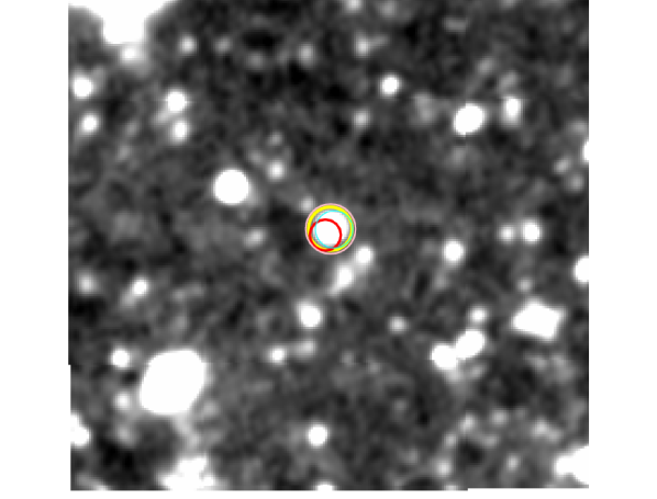
We used the $Swift$-XRT positions to cross-correlate our sources with multiple catalogs, selected in different bands. See Fig. 1 Based on the $Swift$-XRT typical positional accuracy, we allowed a maximum position uncertainty of 5^′′, except for the cross-correlation with the ROSAT catalog (1RXS, Voges et al., 1999, see below). The resulting associations are presented in Table 6. The different catalogs used for the association are reported in the following sections.

3.1 1RXS

The ROSAT All-Sky Survey Source Catalogs for bright and faint sources (1RXS Voges et al., 1999, 2000) contain 18806 and 105924 sources, respectively. The positional uncertainties for these sources are of the order of 30 $\,\!\!{}^{\prime\prime}$, therefore, we compare the 1RXS positions with the $Swift$-XRT positions allowing a maximum uncertainty of 30 $\,\!\!{}^{\prime\prime}$to find the possible associations. This lead to 8 positional correlations, as listed in Table 6. The 1RXS positional error is reported in parenthesis for each association in this table.

3.2 BZCat

The 5th Roma-BZCat catalog is the largest known blazar sample (Massaro et al., 2015, 2016). Three out of 52 sources were found spatially coincident with BZCat sources within 5^′′and all of them are classified as BL Lacs: 3FHL J0316.5-2610, 3FHL J1248.8-5128 and 3FHL J1553.8-2425 with redshifts, $z$= 0.443, 0.351 and 0.332, respectively.

3.3 AllWISE

We cross-correlated our sample with AllWISE, the complete Wide-field Infrared Survey Explorer (WISE) point source catalog (Cutri & al., 2013), and WIBRaLS, a catalog of radio-loud candidate $\gamma$-ray emitting blazars with WISE colors similar to the colors of confirmed $\gamma$-ray blazars (D’Abrusco et al., 2014). 39 sources were found coincident with AllWISE positions and 3 identified as BL Lacs in the WIBRals catalog, which are the same found in BZCat. (see Table 6). 31 of these sources were detected in all the W1, W2, W3 and W4 filters (3.4, 4.6, 12 and 22 $\mu$m, respectively). However, only upper limits for W3 and W4 were provided for 8 sources. See Fig. 2

3.3.1 WISE color index classification

Massaro et al. (2012) introduced a method to identify blazars of uncertain type using a four-filters WISE color-color diagram (Sharma & Chauhan, 2011). These authors identified a particular region in the diagram, which separates blazars from other source classes. They termed this region the WISE blazar strip (WBS) (see Fig 1, 2 in Massaro et al., 2012). Moreover, they found that BL Lacs and FSRQs follow a bimodal distribution, such that the former occupy the bluer part of the color-color diagram. Utilizing the information obtained from the spatial correlation with the AllWISE catalog in our sample of 39 sources with WISE counterpart, we compare their position on the WISE color-color plot with that of the 915 known blazars from the 3FHL catalog. It is evident from Fig. 2 that $>$80% of our sources lie within the WISE Gamma-ray Strip Projections (Massaro et al., 2012) for BL Lacs and FSRQs; and the majority of these occupy the BL Lac region.

3.4 Million Quasar catalog

The catalog published by Flesch & W. (2017) presents type I and II QSOs , AGNs and BL Lacs reported in various catalogs from the literature before 21 June, 2016. This list also includes the candidates based on the SDSS photometric quasar catalogs. Ten sources in our sample have an association in the Million Quasar catalog: two were coincident with QSO type I, three with BL Lacs and the other five with possible QSOs with likelihood $>$85%. Finally, the match to the Million Quasar catalog yielded redshifts for two sources (see Table 6). These redshifts were derived using the photometric method utilizing the SDSS DR12 catalog (Alam et al., 2015), details of which are provided in the Half Million Quasar catalog (Flesch & W., 2015). Seven of these ten sources are also spatially coincident with a radio counterpart.

3.5 6dFGS

The 6dF Galaxy Survey (6dFGS) catalog (Jones et al., 2009) provides the redshift map of the Southern hemisphere for nearby objects ($z$ $\lesssim$ 0.1). None of the sources in this catalog are positionally coincident with our sample sources within a 5^′′ uncertainty radius circle.

3.6 Radio catalogs

3.6.1 NVSS

The NRAO VLA Sky Survey (NVSS) (Condon et al., 1998) constitutes the radio observations of celestial objects with declination greater than -40 $\deg$ at 1.4 GHz. The radio positions of the 22 counterparts of the 3FHL sources is presented in Table 6.

3.6.2 SUMSS

The Sydney University Molonglo Sky Survey (Mauch et al., 2003, SUMSS;) with radio observations at 843 MHz consists of Southern Hemisphere objects. Two sources in our sample have a radio counterpart in this catalog (see Table 6).

3.6.3 2WHSP

Chang et al. (2016) assembled the largest known catalog of WISE High Synchrotron Peak blazars (2WHSP) which comprises 1691 sources. These authors cross-correlated AllWISE catalog with various other wavelength surveys (radio, IR, X-ray). Utilizing this multiwavelength information, they identified blazars, calculated their peak synchrotron frequencies ($\nu_{syn}^{pk}$) and listed the HSPs ($\nu_{syn}^{pk}$ $>$ 15 Hz) in the 2WHSP catalog. We found 9 sources from our sample to be spatially coincident with HSP blazars in this catalog. The 2WHSP identifications of these sources are provided in Table 6.

3.7 Miscellaneous

Finally, we checked for potential counterparts using the two largest online databases of astronomical objects, i.e., SIMBAD (Wenger et al., 2000) and the NASA/IPAC Extragalactic Database (NED). We found the following possible associations, which were not found in any of the above mentioned catalogs:

3FHL J0438.0-7328, 3FHL J1249.2-2809: These two sources are positionally coincident with galaxies LEDA 255538 and LEDA 745327, respectively. These associations are derived from HYPERLEDA, a catalog of about one million galaxies brighter than B=18 mag (Paturel et al., 2003). No redshift information was found for these two objects.

3FHL J1234.8-0435: This 3FHL source spatially coincides with a galaxy listed in the 2dF Galaxy Redshift Survey Colless et al. (2001). The redshift, $z$=0.277, provided by this catalog was obtained from both absorption and emission features.

4 Classification with machine learning

Multiwavelength data analysis is typically required for every Fermi detected source to be correctly classified. This process is highly time consuming and the lack of this information has led to an increasing fraction of unidentified sources in every new Fermi catalog release. However, $\sim$ 80% of the objects in the 3FHL catalog are associated with blazars (FSRQ, BL Lac or BCU), and this fraction increases to $\sim$ 90% if sources along the Galactic plane ($|b|\leq 10^{\circ}$) are not considered. In our sample, 36 out of 52 sources are high-latitude objects, therefore we assume that all these 36 unknown sources in our sample are blazars. This assumption is also justified by the fact that, as seen in Fig. 2, most of the sources are coincident with the WISE-blazar strip, except three outliers: 3FHL J0427.5-6705 (W3 measurement S/N=0.1, no radio), 3FHL J1650.9+0430 (W3 measurement S/N =0.1, no radio) and 3FHL J1958.1+2437.
Although it is quite evident from Fig. 2 that most of our sources lie within the blazar region, in particular, BL Lac region, these results are based on only two parameters. We thus further analyze our findings by employing various other properties, to refine the way in which we differentiate BL Lacs from FSRQs. In order to accomplish this multi-parameter space classification, we employ three different machine learning algorithms. The parameters employed in these methods were derived from the 3FGL, 1SXPS (Evans et al., 2014) and AllWISE catalogs, and are discussed in detail in Section 4.4. Various machine learning techniques have been successfully applied to $Fermi$ unidentified sources, e.g., Ackermann et al. (2012); Mirabal et al. (2012, 2016); Saz Parkinson et al. (2016); Salvetti et al. (2017). From a wide variety of available methods used by these authors, we chose to apply three most commonly employed methods: Decision Tree (Quinlan & Shapiro, 1990), Support Vector Machines (Hearst et al., 1998) and Random Forest (Breiman, 2001).

4.1 Decision Tree

The decision tree classifier (DT) is an example of supervised machine learning algorithm which separates a dataset into two or more categories based on certain parameters associated with the input data. The data is continuously split into nodes and branches until every data point is assigned to one or the other category. The decision of splitting into separate nodes is based on the Gini index, an impurity measurement. The Gini impurity parameter provides a measurement of the probability of incorrectly labeling a randomly chosen element in the given dataset. The decision tree algorithm works towards minimizing this value and splits the sample into branches until this index reaches zero. Mathematically, it is defined as

$$G=1-\Sigma_{i=1}^{J}p_{i}^{2}$$

which calculates the Gini impurity for a dataset with $J$ categories with $p_{i}$ being the fraction of items labeled with category $i$ in the sample. Higher values of G imply higher inequality between two classes for a given parameter. The decision tree is split until the Gini index reaches a minimum value equal to zero, thereby assigning a particular class to the underlying items. This method employs a dataset with known classification as training dataset and trains the classifier. The accuracy obtained for a trained dataset is calculated to evaluate its usage on a sample with no classification.

4.2 Support Vector Machines

Support Vector Machine (SVM) is another supervised learning method for separating a dataset into two categories. The underlying principle for this method is that for any data point, $i$ or $j$ (two categories), one or a set of maximum margin hyperplane are found such that the distance between this plan and the nearest point in either category is maximized.

Mathematically, a hyperplane for a set of points with category , $i$ (say $\vec{x}$) is defined as following:

$$\vec{w}.\vec{x}-b=0,$$

such that the parameter $\frac{b}{||\vec{w}||}$ defines the distance of this plane from the origin along $\vec{w}$, where $\vec{w}$ is the normal vector to the hyperplane. This is an example of linear kernel classification for SVM. A non-linear SVM employs polynomial or rbf kernels to classify any dataset for higher dimensions. In the context of our work, we employ a polynomial kernel and a non-linear SVM to classify the sample into two kind of blazars, i.e., BL Lacs or FSRQs.

4.3 Random Forest

A random forest is one of the most commonly employed supervised machine learning method used for both classification and regression analysis. A random forest classifier operates as an ensemble algorithm based on the principle of a decision tree classifier. This method constructs various decision tree algorithms and assigns a class to a source for every iteration. An aggregate of these predicted classes is assigned as the final resulting class for that particular source. This method has an advantage over running a single decision tree, since it utilizes the multitude of decision trees, thereby solving the problem of overfitting (Hastie et al., 2009), which is usually observed in the latter case. We employ this method to classify our sample into BL Lacs and/or FSRQs. This yields probabilities for each source to be associated as a BL Lac or an FSRQ.

4.4 Sample and Parameter Section

We employed the DT classifier, SVM classifier and Random Forest implemented in sklearn0.20.0 library (Pedregosa et al., 2011) in python 2.7 on a sample of 152 3FHL blazars (115 BLLacs and 37 FSRQs). This sample was chosen as a subset of all the BL Lacs and FSRQs in the 3FHL catalog for which all the six parameters listed in Table LABEL:tab:pars were available. The reason for the selection of these six properties was based on the fact that these have been observed to distinguish BL Lacs from FSRQs. In general, BL Lacs exhibit harder spectrum in Gamma-rays (e.g. Abdo et al. (2010); Ackermann et al. (2015)) and softer in X-rays (e.g. Donato et al. (2001)) as compared to FSRQs , therefore, we select the spectral indices in Gamma-ray (3FHL and 3FGL) and X-ray. The WISE colors, as already discussed in the text, clearly differentiate the two classes of blazars. FSRQs can be distinguished from BL Lacs on the basis of variability. In the 3FHL catalog (Ajello et al., 2017), a parameter called Variability Bayes Blocks is provided, which lists the number of Bayesian blocks from variability analysis. The values of this parameter range from -1 to 15, where -1 implies no variability and 15 implies high variability. FSRQs exhibit higher values for this parameter, implying higher variability as compared to BL Lacs. This sample was divided into training and test datasets in order to check the accuracy of the method employed. The training and test datasets comprised of 102 blazars (77 BL Lacs and 25 FSRQs) and 50 blazars (38 BL Lacs and 12 FSRQs), respectively. Since the total sample contains $\sim$ 75% BL Lacs and only 25% FSRQs, which being highly imbalanced could yield inaccurate results biased towards the major class, when a machine learning method is applied. We, therefore, employed a technique called SMOTE (Synthetic Minority Over-sampling Technique) (Chawla et al., 2002). This method creates synthetic minority class using k nearest neighbors algorithm, thereby generating equal number of sources in each class. An an example, in this case, the training dataset has 77 BL Lacs and 25 FSRQs. Implementation of SMOTE method generated 52 synthetic FSRQs, thereby balancing the two classes (77 sources for each class) before application of a classification method.

5 Results

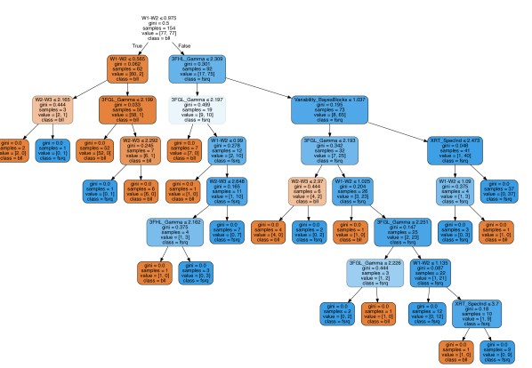
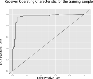
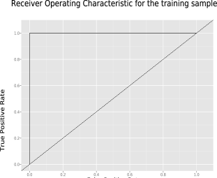
The resulting decision tree from the training sample is shown in Fig. 3. We employed this trained classifier on the test dataset (38 BL Lacs and 12 FSRQs) which yielded an accuracy of 86%. This classifier was then applied to the unknown 3FHL sample, which yielded results suggesting that 31 out of the 36 high-latitude unassociated sources are BL Lacs and the rest are FSRQs. For SVM, a receiver operating characteristic curve (ROC) is used to evaluate the accuracy of this binary classifier and it is shown in Fig. 4. The ROC is constructed by plotting the true positive rate (TPR, number of correct positive results) against the false positive rate (FPR, number of incorrect positive results) at various thresholds. The classification accuracy is $\sim$ 90% which was evaluated as the area below the curve for the given sample. The SVM analysis on our sample suggests that all the unknown sources are likely BL Lacs. The Random Forest classifier yielded results consistent with the SVM classifier suggesting that all the unassociated 36 high-latitude sources are BL Lacs. The accuracy obtained on the test sample in this case was 98%. The receiver operating characteristic curves for both the training and the test sample are shown in Fig. 5. A comparison of the results yielded by all these methods is displayed in Table LABEL:tab:mlcomp.

6 Discussion and Conclusions

The immediate objective of this work was to identify the nature of unassociated sources reported in the latest $Fermi$ high energy catalog, the 3FHL. In an attempt to find associations to these sources, $Swift$ HEASARC archive was used to derive the accurate positions of the sources for which data were available, which lead to a sample of 52 3FHL unassociated sources with a single bright X-ray counterpart. The X-ray source positions were cross-matched with various catalogs from radio to X-ray wavelengths (see Section 3), leading to the identification of the likely counterpart for 12 out of the 52 objects (6 out of 52 objects are identified as QSOs, 3 as BL Lacs and 3 as galaxies). Six of these 12 sources also have confirmed redshift measurements ranging from $z$=0.277 to $z$=2.1. In addition, the WISE color-color plot, as shown in Fig. 2, suggests that majority of the 3FHL sources are likely blazars. Moreover, 90% of the high-latitude $|b|\geq$ 10^∘ objects in the 3FHL sample are associated with the blazar population. 36 objects from our source sample are high-latitude objects and assuming that this subsample comprises only blazars, we employed machine learning techniques (DT, SVM and RF) to classify these objects into two kind of blazars, i.e., BL Lacs and FSRQs. The DT classifier yielded results showing that 31 of the high-latitude sources are BL Lacs. The SVM and the RF classifier predict that all these sources are BL Lacs. For details, please see Table LABEL:tab:mlcomp. The inconsistency between the results from DT vs SVM/RF could be attributed to potential overfitting in the former method as discussed earlier.
In nutshell, this work provides classification for 36/200 sources, which reduces the incompleteness of the 3FHL by 18%. While the redshift info is scarce (12%), our group is working on an optical spectroscopic campaign to observe these unassociated sources with 4m and 8m class telescopes, to obtain redshifts for a significant fraction of them and confirm their nature (see Marchesi et al. (2018), where the first results of this campaign are reported). In addition, our recent successful proposal (Swift Cycle 14, prop ID 1417063 PI: Ajello) in an effort to obtain more XRT sources for the unknown/unassociated 3FHL sources is currently in progress. All these continuing studies will drastically reduce the incompleteness of the 3FHL catalog in a few years timescale.

Figure 1: Optical image centered on 3FHL J0121.9-3917 position ( 2.5 $\times$ 2.5 arcmin in size). The positions of counterparts from different catalogs are show with circles of different colors, as follows. NVSS: red; $Swift$-XRT: cyan; 2MASS: magenta; WISE: yellow. The size of each circle is adjusted to display all the catalogs clearly.

Figure 2: WISE color-color diagram for all the known blazars in the 3FHL catalog following the technique introduced by Massaro et al. (2012). The $blue$, $red$, $orange$ circles represent BL Lacs, FSRQs and BCUs, respectively. The $green$ circles represent our sample of 52 sources from the 3FHL data. The two boxes represent the WISE Gamma-ray Strip Projection for BZBs (BL Lacs) ($left$) and BZQs (FSRQs) ($right$), as described in Massaro et al. (2012). This plot clearly suggests that the majority of the sources in our sample are likely to be BL Lacs. The $green$ arrows represent 3FHL unassociated sources for which only an upper limit was provided for the W3 (12 $\mu$m) filter.

Figure 3: The Decision Tree for the training data set which contains 77 BL Lacs and FSRQs, each, employed six parameters based on known distinct properties of two kind of blazars.

(a)

(b)

Figure 4: The SVM method generated ROC curves for the (a) training sample and the (b) test sample. The test sample yielded an accuracy score 90%. The straight diagonal line in both the plots represent the non-discriminatory curve, i.e., if the data points lie on/below this line, the analysis would yield non-diagnostic results.

(a)

(b)

Figure 5: The ROC curves from the Random Forest method for the (a) training sample and the (b) test sample. The test sample yielded an accuracy score 98%. The straight diagonal line in both the plots represent the non-discriminatory curve, i.e., if the data points lie on/below this line, the analysis would yield non-diagnostic results.

Table 1: $Swift$-XRT Analysis

3FHL	RA2000a	Dec2000b	Xray RAc	Xray Decd	Exposure time	Count Rate	$\Gamma_{X}^{e}$	N${}_{H}^{f}$	Fluxg	$\chi^{2}/d.o.f.$
	(hh:mm:ss)	(${}^{\circ}:^{\prime}:^{\prime\prime}$)	(hh:mm:ss)	(${}^{\circ}:^{\prime}:^{\prime\prime}$)	(sec)	(cts s${}^{-}1$)		(cm-2)	(erg cm-2s-1)
J0049.0+4224	00:49:05	+42:24:12	00:48:59.14	+42:23:47.40	4106	1.216	2.54$\pm$0.24	0.12	0.68	48.31/47∗
J0121.9$-$3917	01:21:56	$-$39:17:13	01:21:52.51	$-$39:15:44.64	5736	0.080	1.79$\pm$0.08	0.02	3.45	19.21/19
J0156.2$-$2419	01:56:16	$-$24:19:30	01:56:24.31	$-$24:20:06.72	17280	0.012	2.59$\pm$0.13	0.01	0.98	5.13/9
J0213.9$-$6950	02:13:58	$-$69:50:12	02:13:58.44	$-$69:51:38.16	4098	0.100	1.87$\pm$0.08	0.05	4.44	17.31/17
J0251.2$-$1830	02:51:13	$-$18:30:30	02:51:11.31	$-$18:31:15.57	7572	0.014	2.03$\pm$0.16	0.03	0.64	68.78/88∗
J0316.5$-$2610	03:16:32	$-$26:10:03	03:16:14.95	$-$26:07:57.36	4885	0.152	2.52$\pm$0.06	0.01	4.82	18.90/30
J0350.4$-$5143	03:50:26	$-$51:43:44	03:50:28.37	$-$51:44:54.96	1708	0.160	2.08$\pm$0.13	0.01	6.26	10.12/10
J0350.8$-$2814	03:50:50	$-$28:14:02	03:50:51.34	$-$28:16:33.96	11010	0.068	1.92$\pm$0.06	0.01	3.03	34.24/32
J0401.0$-$5355	04:01:03	$-$53:55:11	04:01:11.45	$-$53:54:56.52	904	0.020	1.95$\pm$0.33	0.01	0.78	11.55/15∗
J0427.5$-$6705	04:27:35	$-$67:05:49	04:27:49.51	$-$67:04:34.68	14500	0.008	$\cdots$	0.04	$\cdots$	$\cdots$ $\dagger$
J0438.0$-$7328	04:38:05	$-$73:28:26	04:38:37.30	$-$73:29:22.20	3868	0.007	2.10$\pm$0.42	0.09	0.19	13.89/25
J0506.9+0323	05:06:55	+03:23:42	05:06:50.09	+03:23:59.28	17280	0.012	2.47$\pm$0.15	0.07	0.57	3.7/7∗
J0541.1$-$4855	05:41:10	$-$48:55:40	05:41:07.03	$-$48:54:10.45	1224	0.008	2.04$\pm$0.76	0.03	0.47	3.8/8∗
J0559.6+3045	05:59:40	+30:45:44	05:59:40.42	+30:42:32.75	4680	0.004	2.04$\pm$0.76	0.36	0.48	9.6/18∗
J0706.1+0247	07:06:08	+02:47:55	07:06:10.86	+02:44:50.82	2432	0.038	1.88$\pm$0.23	0.36	2.91	68.18/74∗
J0725.7$-$0548	07:25:44	$-$05:48:53	07:25:47.69	$-$05:48:27.00	4872	0.036	2.37$\pm$0.18	0.26	2.39	10.22/6
J0739.7$-$6720	07:39:45	$-$67:20:09	07:39:27.74	$-$67:21:37.04	3192	0.041	2.05$\pm$0.16	0.09	2.36	82.00/96∗
J0747.7$-$4927	07:47:44	$-$49:28:00	07:47:25.30	$-$49:26:32.64	4086	0.023	2.44$\pm$0.18	0.09	1.18	66.75/71∗
J0813.7$-$0353	08:13:46	$-$03:53:57	08:13:38.02	$-$03:57:17.64	3157	0.066	1.71$\pm$0.15	0.05	3.37	5.89/7
J0820.2$-$2803	08:20:15	$-$28:03:04	08:20:14.69	$-$28:03:03.60	1763	0.022	2.49$\pm$0.35	0.27	1.95	26.96/36∗
J0928.5$-$5256	09:28:33	$-$52:56:05	09:28:18.98	$-$52:57:05.40	3579	0.006	$\cdots$	0.94	$\cdots$	$\cdots$ $\dagger$
J0937.8$-$1434	09:37:52	$-$14:34:16	09:37:54.86	$-$14:33:43.56	4480	$\cdots$	$\cdots$	0.05	$\cdots$	$\cdots$ $\dagger$
J1016.2$-$4245	10:16:14	$-$42:45:34	10:16:21.02	$-$42:47:24.36	3883	0.020	2.39$\pm$0.19	0.05	0.89	54.36/65∗
J1024.5$-$4543	10:24:33	$-$45:43:47	10:24:32.78	$-$45:44:27.96	4158	0.057	2.48$\pm$0.13	0.12	2.87	81.9/70
J1033.4$-$5033	10:33:26	$-$50:33:39	10:33:32.28	$-$50:35:28.68	3836	0.029	2.25$\pm$0.17	0.19	1.78	83.36/98∗
J1034.8$-$4645	10:34:53	$-$46:45:09	10:34:38.45	$-$46:44:01.92	1733	0.063	1.97$\pm$0.19	0.14	3.40	3.36/4
J1047.9$-$3738	10:47:56	$-$37:38:41	10:47:57.02	$-$37:37:35.76	3621	0.022	2.49$\pm$0.20	0.04	1.00	49.22/67∗
J1117.2$-$5338	11:17:15	$-$53:38:03	11:17:14.74	$-$53:38:15.04	3361	0.012	1.97$\pm$0.33	0.15	0.85	40.52/37∗
J1125.0$-$5806	11:25:05	$-$58:06:42	11:25:04.49	$-$58:05:40.78	3094	0.019	2.49$\pm$0.24	0.37	2.15	58.74/55∗
J1145.9$-$0637	11:45:54	$-$06:37:18	11:46:00.65	$-$06:38:51.36	2343	0.024	1.98$\pm$0.24	0.03	3.01	54.65/48∗
J1220.1$-$2459	12:20:11	$-$24:59:07	12:20:14.54	$-$24:59:52.08	4233	0.061	2.00$\pm$0.12	0.08	3.07	9.56/10∗
J1220.4$-$3714	12:20:26	$-$37:14:31	12:20:19.78	$-$37:14:10.68	1354	0.051	2.35$\pm$0.20	0.08	2.43	39.28/54∗
J1234.8$-$0435	12:34:50	$-$04:35:11	12:34:47.96	$-$04:32:46.26	3424	0.007	2.15$\pm$0.29	0.03	0.29	22.67/23∗
J1240.5$-$7148	12:40:36	$-$71:48:40	12:40:21.19	$-$71:48:57.24	4695	0.272	1.84$\pm$0.04	0.14	14.98	78.43/55∗
J1248.8+5128	12:48:54	+51:28:08	12:48:34.30	+51:28:06.96	6832	0.010	1.83$\pm$0.20	0.01	0.47	17.25/21∗
J1249.2$-$2809	12:49:13	$-$28:09:37	12:49:19.42	$-$28:08:38.04	5956	0.101	2.17$\pm$0.07	0.06	4.30	25.68/27
J1447.0$-$2657	14:47:04	$-$26:57:50	14:46:57.41	$-$26:57:01.80	4106	0.239	1.89$\pm$0.05	0.09	13.8	21.88/42
J1517.0+2638	15:17:02	+26:38:31	15:16:49.82	+26:36:42.48	3514	0.005	2.13$\pm$0.46	0.04	0.23	18.49/17∗
J1541.7+1413	15:41:44	+14:13:48	15:41:49.85	+14:14:44.52	2878	0.005	2.61$\pm$0.62	0.03	0.21	16.01/14∗
J1553.8$-$2425	15:53:51	$-$24:25:14	15:53:31.25	$-$24:22:05.16	5384	0.013	1.39$\pm$0.27	0.11	0.92	35.75/60
J1650.9+0430	16:51:00	+04:30:05	16:50:58.87	+04:27:34.92	14020	0.001	$\cdots$	0.06	$\cdots$	$\cdots$ $\dagger$
J1704.5$-$0527	17:04:34	$-$05:27:25	17:04:34.10	$-$05:28:37.92	6309	0.063	1.88$\pm$0.09	0.13	3.56	24.32/18
J1856.1$-$1221	18:56:07	$-$12:21:16	18:56:06.67	$-$12:21:50.40	3286	0.023	1.93$\pm$0.28	0.16	1.63	21.00/21∗
J1958.1+2437	19:58:07	+24:37:51	19:58:00.38	+24:38:03.84	3529	0.019	2.39$\pm$0.30	0.69	3.13	59.42/55∗
J2036.0+4901	20:36:03	+49:01:11	20:35:51.24	+49:01:39.72	3521	0.004	2.01$\pm$1.17	0.66	0.13	16.01/11∗
J2042.7+1520	20:42:45	+15:20:03	20:42:59.71	+15:21:06.48	17600	0.035	2.23$\pm$0.08	0.07	1.89	29.92/26
J2109.7+0440	21:09:42	+04:40:11	21:09:40.08	+04:39:59.40	354	0.025	1.58$\pm$0.73	0.07	1.69	6.19/6∗
J2115.2+1218	21:15:15	+12:18:29	21:15:22.10	+12:18:02.88	3756	0.007	2.95$\pm$0.36	0.05	0.37	21.28/25∗
J2142.3+3659	21:42:22	+36:59:40	21:42:26.50	+36:59:48.12	4365	0.022	2.16$\pm$0.14	0.17	6.73	6.69/7
J2142.7+1959	21:42:44	+19:59:22	21:42:47.45	+19:58:09.84	1628	0.123	2.99$\pm$0.22	0.07	1.88	64.00/69∗
J2151.5+4155	21:51:32	+41:55:47	21:51:22.90	+41:56:32.28	3284	0.022	2.81$\pm$0.32	0.23	1.53	26.37/62
J2308.8+5424	23:08:54	+54:24:22	23:08:48.62	+54:26:08.88	1051	0.022	2.24$\pm$0.53	0.28	2.11	18.41/20∗

Note. — Sources with $\dagger$ sign did not yield a reliable fit with a simple powerlaw model.

Table 2: Cross-Correlation

3FHL	1RXS	Radio	WISE	BZ Cat	MILLIQUAS	2WHSP	Class	Redshift
J0049.0+4224	$\cdots$	N J004859+422350	J004859.15+422351.1	$\cdots$	$\cdots$	004859.0+422351	$\cdots$	$\cdots$
J0121.9$-$3917	$\cdots$	S J012152$-$391542	J012152.69$-$391544.2	$\cdots$	$\cdots$	$\cdots$	$\cdots$	$\cdots$
J0156.2$-$2419	$\cdots$	$\cdots$	J015624.54$-$242003.7		J015624.6$-$242004	$\cdots$	QSO 93%	$\cdots$
J0213.9$-$6950	$\cdots$	$\cdots$	J021358.69$-$695137.0	$\cdots$	$\cdots$	$\cdots$	$\cdots$	$\cdots$
J0251.2$-$1830	$\cdots$	N J025111$-$183112	J025111.52$-$183112.7	$\cdots$	$\cdots$	$\cdots$	$\cdots$	$\cdots$
J0316.5$-$2610	$\cdots$	N J031615$-$260755	J031614.94$-$260757.2	J0316$-$2607	RXS J03162$-$2607	031614.8-260757	BL LAC	0.443
J0350.4$-$5143	$\cdots$	$\cdots$	J035028.30$-$514454.3	$\cdots$	$\cdots$	$\cdots$	$\cdots$	$\cdots$
J0350.8$-$2814	$\cdots$	$\cdots$	J035051.32$-$281632.8	$\cdots$	$\cdots$	035051.2-281632	$\cdots$	$\cdots$
J0401.0$-$5355	$\cdots$	$\cdots$	J040111.20$-$535458.5	$\cdots$	J040111.2$-$535458	$\cdots$	QSO 86%	$\cdots$
J0427.5$-$6705	$\cdots$	$\cdots$	J042749.72$-$670434.7	$\cdots$	$\cdots$	$\cdots$	$\cdots$
J0438.0$-$7328	$\cdots$	S J043836$-$732921	J043837.07$-$732921.6	$\cdots$	$\cdots$	$\cdots$	LEDA 255538	$\cdots$
J0506.9+0323	$\cdots$	N J050650+032401	J050650.14+032358.7	$\cdots$	$\cdots$	$\cdots$	$\cdots$
J0541.1$-$4855	$\cdots$	$\cdots$	J054106.92$-$485410.3	$\cdots$	J054106.9$-$485412	$\cdots$	QSO 91%	$\cdots$
J0559.6+3045	$\cdots$	N J055941+304227		$\cdots$	$\cdots$	$\cdots$	$\cdots$	$\cdots$
J0706.1+0247	$\cdots$	N J070610+024449	$\cdots$	$\cdots$	$\cdots$	$\cdots$	$\cdots$	$\cdots$
J0725.7$-$0548	$\cdots$	$\cdots$	$\cdots$	$\cdots$	$\cdots$	$\cdots$	$\cdots$	$\cdots$
J0739.7$-$6720	J073928.1$-$672147(15)	$\cdots$		$\cdots$	$\cdots$	$\cdots$	$\cdots$	$\cdots$
J0747.7$-$4927	J074725.1$-$492626(12)	$\cdots$	J074724.74-492633.1	$\cdots$	$\cdots$	074724.7-492633	$\cdots$	$\cdots$
J0813.7$-$0353	$\cdots$	N J081338$-$035716	J081338.07$-$035716.7	$\cdots$	$\cdots$	$\cdots$	$\cdots$	$\cdots$
J0820.2$-$2803	$\cdots$	$\cdots$	$\cdots$	$\cdots$	$\cdots$	$\cdots$	$\cdots$	$\cdots$
J0928.5$-$5256	$\cdots$	$\cdots$	J092818.63$-$525703.1	$\cdots$	$\cdots$	$\cdots$	$\cdots$	$\cdots$
J0937.8$-$1434	$\cdots$	$\cdots$	$\cdots$	$\cdots$	$\cdots$	$\cdots$	$\cdots$	$\cdots$
J1016.2$-$4245	J101620.6$-$424733(14)	$\cdots$	J101620.67$-$424722.6	$\cdots$	$\cdots$	$\cdots$	$\cdots$	$\cdots$
J1024.5$-$4543	$\cdots$	$\cdots$	J102432.37$-$454426.9	$\cdots$	$\cdots$	$\cdots$	$\cdots$	$\cdots$
J1033.4$-$5033	J103332.0$-$503539(14)		J103332.15$-$503528.8	$\cdots$	$\cdots$	$\cdots$	$\cdots$	$\cdots$
J1034.8$-$4645	$\cdots$	$\cdots$	J103438.49$-$464403.5	$\cdots$	$\cdots$	$\cdots$	$\cdots$	$\cdots$
J1047.9$-$3738	$\cdots$	$\cdots$	J104756.94$-$373730.8	$\cdots$	$\cdots$	104756.8-373730	$\cdots$	$\cdots$
J1117.2$-$5338	$\cdots$	$\cdots$	$\cdots$	$\cdots$	$\cdots$	$\cdots$	$\cdots$	$\cdots$
J1125.0$-$5806	J112502.3$-$580547(16)	$\cdots$	J112503.99$-$580539.9	$\cdots$	$\cdots$	$\cdots$	$\cdots$	$\cdots$
J1145.9$-$0637	$\cdots$	$\cdots$	J114600.85$-$063854.9	$\cdots$	$\cdots$	$\cdots$	$\cdots$	$\cdots$
J1220.1$-$2459	$\cdots$	N J122014$-$245949	J122014.53$-$245948.6	$\cdots$	J122014.5$-$245948	$\cdots$	$\cdots$	$\cdots$
J1220.4$-$3714	$\cdots$	N J122020$-$371411	J122019.81$-$371414.2	$\cdots$	$\cdots$	122019.8-371413	$\cdots$	$\cdots$
J1234.8$-$0435	$\cdots$	$\cdots$	J123448.05$-$043245.2	$\cdots$	$\cdots$	$\cdots$	Galaxy	0.277
J1240.5$-$7148	J124015.2$-$714859(21)	$\cdots$	J124021.21$-$714857.7	$\cdots$	$\cdots$	$\cdots$	$\cdots$	$\cdots$
J1248.8+5128	J124832.1+512817(12)	N J124834+512807	J124834.29+512807.8	J1248+5128	SDSS J124834.30+512807.8	$\cdots$	BL LAC	0.351
J1249.2$-$2809	$\cdots$	N J124919$-$280833	J124919.31$-$280834.4	$\cdots$	$\cdots$	124919.3-280834	LEDA 745327	$\cdots$
J1447.0$-$2657	$\cdots$	$\cdots$	$\cdots$	$\cdots$	$\cdots$	$\cdots$	$\cdots$	$\cdots$
J1517.0+2638	$\cdots$	$\cdots$	$\cdots$	$\cdots$	$\cdots$	$\cdots$	$\cdots$	$\cdots$
J1541.7+1413	$\cdots$	$\cdots$	$\cdots$	$\cdots$	$\cdots$	$\cdots$	$\cdots$	$\cdots$
J1553.8$-$2425	$\cdots$	N J155331.6$-$242206	$\cdots$	$\cdots$	PKS 1550$-$242	$\cdots$	BL Lac	0.332
J1650.9+0430	$\cdots$	$\cdots$	J165058.69+042734.9	$\cdots$	$\cdots$	$\cdots$	$\cdots$	$\cdots$
J1704.5$-$0527	$\cdots$	$\cdots$	J170433.83$-$052840.7	$\cdots$	$\cdots$	170433.7-052840	$\cdots$	$\cdots$
J1856.1$-$1221	$\cdots$	N J185606$-$122148	$\cdots$	$\cdots$	$\cdots$	$\cdots$	$\cdots$	$\cdots$
J1958.1+2437	$\cdots$	N J195800+243802	J195800.50+243800.9	$\cdots$	$\cdots$	$\cdots$	$\cdots$	$\cdots$
J2036.0+4901	$\cdots$	N J203551+490143	$\cdots$	$\cdots$	$\cdots$		$\cdots$	$\cdots$
J2042.7+1520	$\cdots$	N J204259+152107	J204259.72+152108.1	$\cdots$	J204259.7+152108		QSO 81	$\cdots$
J2109.7+0440	$\cdots$	N J210939+044000	J210940.12+044000.6	$\cdots$	SDSS J210940.12+044000.3		QSO TYPE 1	1.4†
J2115.2+1218	$\cdots$	N J211522+121802	J211522.00+121802.6	$\cdots$	SDSS J211522.00+121802.8	$\cdots$	QSO TYPE 1	2.1†
J2142.3+3659	$\cdots$	N J214226+365949	J214226.49+365949.7	$\cdots$	$\cdots$	214226.4+365948	$\cdots$	$\cdots$
J2142.7+1959	$\cdots$	N J214247+195810	J214247.62+195810.9	$\cdots$	$\cdots$	$\cdots$	$\cdots$	$\cdots$
J2151.5+4155	$\cdots$	N J215122+415632	J215123.22+415633.9	$\cdots$	$\cdots$	$\cdots$	$\cdots$	$\cdots$
J2308.8+5424	$\cdots$	N J230848+542612	J230848.74+542611.2	$\cdots$	$\cdots$	$\cdots$	$\cdots$	$\cdots$

Note. — The redshifts marked with $\dagger$ were derived using a clustering method based on the photometric SDSS data. See Flesch & W. (2015) for details.

References. — ^aDAbrusco2014, ^bFlesch2015, ^cFlesch2017, ^dMassaro2015a, ^ePaturel2003, ^fColless2001

Table 3: Parameters for Blazars for classification

Parameter	Catalog	References
X-ray Spectral Index	Table 1 for unknown sample	See Table 1
	1SXPS for training set	Evans et al. (2014)
Variability Bayes Blocks	3FHL	Ajello et al. (2017)
w1-w2	AllWISE	Cutri & al. (2013)
w2-w3	AllWISE	Cutri & al. (2013)
Gamma-ray Spectral Index 1	3FGL	Acero et al. (2015)
Gamma-ray Spectral Index 2	3FHL	Ajello et al. (2017)

Table 4: Machine Learning Results

3FHL	DT Pred	SVM Pred	SVM Prob	RF Pred	RF Prob
J0049.0+4224	fsrq	bll	1.0	bll	0.84
J0121.9-3917	bll	bll	1.0	bll	0.85
J0156.2-2419	bll	bll	0.94	bll	0.96
J0213.9-6950	bll	bll	0.98	bll	0.69
J0251.2-1830	bll	bll	0.95	bll	0.99
J0316.5-2610	bll	bll	0.98	bll	0.99
J0350.4-5143	bll	bll	0.98	bll	0.92
J0350.8-2814	bll	bll	1.0	bll	0.85
J0401.0-5355	fsrq	bll	0.99	bll	0.8
J0427.5-6705	fsrq	bll	1.0	bll	0.81
J0438.0-7328	bll	bll	1.0	bll	0.79
J0506.9+0323	bll	bll	0.98	bll	0.95
J0541.1-4855	fsrq	bll	1.0	bll	0.77
J0739.7-6720	bll	bll	1.0	bll	0.74
J0747.7-4927	bll	bll	1.0	bll	0.88
J0813.7-0353	bll	bll	1.0	bll	0.85
J0937.8-1434	bll	bll	1.0	bll	0.9
J1016.2-4245	bll	bll	0.98	bll	1.0
J1047.9-3738	bll	bll	0.98	bll	0.91
J1145.9-0637	bll	bll	1.0	bll	0.84
J1220.1-2459	bll	bll	0.99	bll	0.87
J1220.4-3714	bll	bll	0.98	bll	1.0
J1234.8-0435	bll	bll	0.57	bll	0.93
J1248.8+5128	bll	bll	0.87	bll	0.95
J1249.2-2809	bll	bll	1.0	bll	0.86
J1447.0-2657	bll	bll	0.99	bll	0.73
J1517.0+2638	bll	bll	1.0	bll	0.84
J1541.7+1413	bll	bll	1.0	bll	0.86
J1553.8-2425	bll	bll	0.98	bll	0.84
J1650.9+0430	fsrq	bll	1.0	bll	0.77
J1704.5-0527	bll	bll	0.95	bll	0.97
J2042.7+1520	bll	bll	0.99	bll	0.84
J2109.7+0440	bll	bll	0.99	bll	0.88
J2115.2+1218	bll	bll	0.89	bll	0.97
J2142.3+3659	bll	bll	1.0	bll	0.84
J2142.7+1959	bll	bll	0.99	bll	0.87

• Predicted Class by the Decision Tree Algorithm

• Predicted Class by the SVM Algorithm

• Probability to be a BLL associated by the SVM Method

• Predicted Class by the Random Forest (RF) Algorithm

• Probability to be a BLL associated by the RF Method

References

- Abdo et al. (2010) Abdo, A. A., Ackermann, M., Agudo, I., et al. 2010, The Astrophysical Journal, 716, 30
- Acero et al. (2015) Acero, F., Ackermann, M., Ajello, M., et al. 2015, The Astrophysical Journal Supplement Series, 218, 23
- Ackermann et al. (2012) Ackermann, M., Ajello, M., Allafort, A., et al. 2012, Astrophysical Journal, 753, arXiv:1108.1202
- Ackermann et al. (2013) —. 2013, The Astrophysical Journal Supplement Series, 209, 34
- Ackermann et al. (2015) Ackermann, M., Ajello, M., Atwood, W. B., et al. 2015, The Astrophysical Journal, 810, 14
- Ackermann et al. (2016a) —. 2016a, The Astrophysical Journal Supplement Series, 222, 5
- Ackermann et al. (2016b) —. 2016b, The Astrophysical Journal Supplement Series, 222, 5
- Ajello et al. (2015) Ajello, M., Gasparrini, D., Sanchez-Conde, M., et al. 2015, The Astrophysical Journal Letters, Volume 800, Issue 2, article id. L27, 7 pp. (2015)., 800, arXiv:1501.05301
- Ajello et al. (2017) Ajello, M., Atwood, W. B., Baldini, L., et al. 2017, The Astrophysical Journal Supplement Series, 232, 18
- Alam et al. (2015) Alam, S., Albareti, F. D., Prieto, C. A., et al. 2015, The Astrophysical Journal Supplement Series, Volume 219, Issue 1, article id. 12, 27 pp. (2015)., 219, arXiv:1501.00963
- Arnaud (1996) Arnaud, K. A. 1996, Astronomical Data Analysis Software and Systems V, 101, 17
- Atwood et al. (2009) Atwood, W. B., Abdo, A. A., Ackermann, M., et al. 2009, Astrophysical Journal, 697, 1071
- Breiman (2001) Breiman, L. 2001, Machine Learning, arXiv:/dx.doi.org/10.1023%2FA%3A1010933404324
- Chang et al. (2016) Chang, Y.-L., Arsioli, B., Giommi, P., & Padovani, P. 2016, Astronomy & Astrophysics, 598, A17
- Chawla et al. (2002) Chawla, N. V., Bowyer, K. W., Hall, L. O., & Kegelmeyer, W. P. 2002, Journal of Artificial Intelligence Research, 16, 321
- Colless et al. (2001) Colless, M., Dalton, G. B., Maddox, S. J., et al. 2001, Monthly Notices of the Royal Astronomical Society, Volume 328, Issue 4, pp. 1039-1063., 328, 1039
- Condon et al. (1998) Condon, J. J., Cotton, W. D., Greisen, E. W., et al. 1998, The Astronomical Journal, 115, 1693
- Cutri & al. (2013) Cutri, R., & al., E. 2013, VizieR Online Data Catalog, 2328, 0
- D’Abrusco et al. (2014) D’Abrusco, R., Massaro, F., Paggi, A., et al. 2014, The Astrophysical Journal Supplement Series, 215, 14
- Domínguez & Ajello (2015) Domínguez, A., & Ajello, M. 2015, The Astrophysical Journal Letters, Volume 813, Issue 2, article id. L34, 4 pp. (2015)., 813, arXiv:1510.07913
- Donato et al. (2001) Donato, D., Ghisellini, G., Tagliaferri, G., & Fossati, G. 2001, Astronomy & Astrophysics, 375, 739
- Evans et al. (2007) Evans, P. A., Tyler, L. G., Beardmore, A. P., & Osborne, J. P. 2007
- Evans et al. (2008) Evans, P. A., Beardmore, A. P., Page, K. L., et al. 2008, Monthly Notices of the Royal Astronomical Society, Volume 397, Issue 3, pp. 1177-1201., 397, 1177
- Evans et al. (2014) Evans, P. A., Osborne, J. P., Beardmore, A. P., et al. 2014, Astrophysical Journal, Supplement Series, 210, arXiv:1311.5368
- Fichtel et al. (1993) Fichtel, C. E., Bertsch, D. L., Dingus, B., et al. 1993, Advances in Space Research, 13, 637
- Flesch & W. (2015) Flesch, E. W., & W., E. 2015, Publications of the Astronomical Society of Australia, Volume 32, id.e010 17 pp., 32, arXiv:1502.06303
- Flesch & W. (2017) —. 2017, VizieR On-line Data Catalog: VII/277. Originally published in: 2015PASA…32…10F, 7277
- Gehrels et al. (2004) Gehrels, N., Chincarini, G., Giommi, P., et al. 2004, The Astrophysical Journal, 611, 1005
- Hassan et al. (2017) Hassan, T., Domínguez, A., Lefaucheur, J., et al. 2017, eprint arXiv:1708.07704, arXiv:1708.07704
- Hastie et al. (2009) Hastie, T., Tibshirani, R., & Friedman, J. 2009, Springer Series in Statistics, doi:10.1007/978-0-387-98135-2
- Hearst et al. (1998) Hearst, M. a., Dumais, S. T., Osman, E., Platt, J., & Scholkopf, B. 1998, …Systems and their …, arXiv:arXiv:1011.1669v3
- Jones et al. (2009) Jones, D. H., Read, M. A., Saunders, W., et al. 2009, Monthly Notices of the Royal Astronomical Society, Volume 399, Issue 2, pp. 683-698., 399, 683
- Kalberla et al. (2005) Kalberla, P. M. W., Burton, W. B., Hartmann, D., et al. 2005, Astronomy and Astrophysics, Volume 440, Issue 2, September III 2005, pp.775-782, 440, 775
- Marchesi et al. (2018) Marchesi, S., Kaur, A., & Ajello, M. 2018, The Astronomical Journal, 156, 212
- Massaro et al. (2016) Massaro, E., Giommi, P., Leto, C., et al. 2016, VizieR On-line Data Catalog: VII/274. Originally published in: 2015Ap&SS.357…75M, 7274
- Massaro et al. (2015) Massaro, E., Maselli, A., Leto, C., et al. 2015, Astrophysics and Space Science, Volume 357, Issue 1, article id.75 4pp., 357, arXiv:1502.07755
- Massaro et al. (2012) Massaro, F., D’Abrusco, R., Tosti, G., et al. 2012, Astrophysical Journal, 750, 138
- Mauch et al. (2003) Mauch, T., Murphy, T., Buttery, H. J., et al. 2003, Monthly Notice of the Royal Astronomical Society, Volume 342, Issue 4, pp. 1117-1130., 342, 1117
- Mirabal et al. (2016) Mirabal, N., Charles, E., Ferrara, E. C., et al. 2016, The Astrophysical Journal, 825, 69
- Mirabal et al. (2012) Mirabal, N., Frías-Martinez, V., Hassan, T., & Frías-Martinez, E. 2012, Monthly Notices of the Royal Astronomical Society: Letters, 424, L64
- Paiano et al. (2017) Paiano, S., Franceschini, A., & Stamerra, A. 2017, Monthly Notices of the Royal Astronomical Society, Volume 468, Issue 4, p.4902-4937, 468, 4902
- Paturel et al. (2003) Paturel, G., Petit, C., Prugniel, P., et al. 2003, Astronomy {&} Astrophysics, 412, 45
- Pedregosa et al. (2011) Pedregosa, F., Weiss, R., & Brucher, M. 2011, Journal of Machine Learning Research, arXiv:1201.0490v1
- Quinlan & Shapiro (1990) Quinlan, G. D., & Shapiro, S. L. 1990, The Astrophysical Journal, 356, 483
- Salvetti et al. (2017) Salvetti, D., Chiaro, G., La Mura, G., & Thompson, D. J. 2017, Monthly Notices of the Royal Astronomical Society, Volume 470, Issue 2, p.1291-1297, 470, 1291
- Saz Parkinson et al. (2016) Saz Parkinson, P. M., Xu, H., Yu, P. L. H., et al. 2016, The Astrophysical Journal, 820, 8
- Sharma & Chauhan (2011) Sharma, S. K., & Chauhan, R. 2011, Current Science, 101, 308
- Stroh & Falcone (2013) Stroh, M. C., & Falcone, A. D. 2013, The Astrophysical Journal Supplement, Volume 207, Issue 2, article id. 28, 12 pp. (2013)., 207, doi:10.1088/0067-0049/207/2/28
- Taylor (2005) Taylor, M. B. 2005, in Astronomical Data Analysis Software and Systems XIV, Vol. 347, 29–+
- Voges et al. (1999) Voges, W., Aschenbach, B., Boller, T., et al. 1999, Astronomy and Astrophysics, v.349, p.389-405 (1999), 349, 389
- Voges et al. (2000) —. 2000, International Astronomical Union Circular, 7432, 1
- Wenger et al. (2000) Wenger, M., Ochsenbein, F., Egret, D., et al. 2000, Astronomy and Astrophysics Supplement, v.143, p.9-22, 143, 9