Elastic Multi-resource Network Slicing:
Can Protection Lead to Improved Performance?

Jiaxiao Zheng, Gustavo de Veciana Dept. of Electrical and Computer Engineering, The University of Texas at Austin, TX gustavo@ece.utexas.edu
Abstract

In order to meet the performance/privacy requirements of future data-intensive mobile applications, e.g., self-driving cars, mobile data analytics, and AR/VR, service providers are expected to draw on shared storage/computation/connectivity resources at the network “edge”. To be cost-effective, a key functional requirement for such infrastructure is enabling the sharing of heterogeneous resources amongst tenants/service providers supporting spatially varying and dynamic user demands. This paper proposes a resource allocation criterion, namely, Share Constrained Slicing (SCS), for slices allocated predefined shares of the network’s resources, which extends traditional αlimit-from𝛼\alpha-fairness criterion, by striking a balance among inter- and intra-slice fairness vs. overall efficiency. We show that SCS has several desirable properties including slice-level protection, envyfreeness, and load driven elasticity. In practice, mobile users’ dynamics could make the cost of implementing SCS high, so we discuss the feasibility of using a simpler (dynamically) weighted max-min as a surrogate resource allocation scheme. For a setting with stochastic loads and elastic user requirements, we establish a sufficient condition for the stability of the associated coupled network system. Finally, and perhaps surprisingly, we show via extensive simulations that while SCS (and/or the surrogate weighted max-min allocation) provides inter-slice protection, they can achieve improved job delay and/or perceived throughput, as compared to other weighted max-min based allocation schemes whose intra-slice weight allocation is not share-constrained, e.g., traditional max-min or discriminatory processor sharing.

I Introduction

Next generation networks face the challenge of supporting data-intensive services and applications, such as self-driving cars, infotainment, augmented/virtual reality [27], Internet of things [6, 27], and mobile data analytics [12, 1]. In order to accommodate the performance and privacy requirements of such services/applications, providers are expected to draw on shared storage/computation/connectivity resources at the network “edge”. Such network systems can take advantage of Software-Defined Networking and Network Function Virtualization technologies to provision slices of shared heterogeneous resources and network functions which are customized to service providers’/tenants’ requirements.

The ability to support slice-based provisioning is central to enabling service providers to take control of managing performance of their own dynamic and mobile user populations. This also improves the scalability by reducing the complexity of performance management on multi-service platforms. The ability to efficiently share network/compute resources is also key to reducing the cost of deploying such services. By contrast with today’s cloud computing platforms, our focus in this paper is on provisioning slices of edge resources to meet mobile users/devices requirements. In general, shared edge resources will have smaller overall capacity resulting in reduced statistical multiplexing and making efficiency critical. Perhaps similarly to cloud computing platforms, providers/tenants will want to make long-term provisioning commitments enabling predictable costs and resource availability, yet benefit, when possible, of elastic resource allocations aligned with spatial variations in their mobile workloads but not at the expense of other slices. Thus a particularly desirable feature is to enable slice-level provisioning agreements which achieve inter-slice protection, load-driven elasticity and network efficiency.

These challenges distinguish our work from previous research in areas including engineering, computer science and economics. The standard framework used in communication networks is utility maximization (see e.g., [29] and references therein), which has led to the design of several transport and scheduling mechanisms and criteria, e.g., the widely discussed proportional fairness. When considering dynamic/stochastic networks, e.g., [4], [17], researchers have studied networks where users are allocated resources based on utility maximization and studied requirements for network stability for ‘elastic’ user demands, e.g., file transfers. This body of work emphasizes user-level resource allocations, without specifically accounting for interactions among slices. Thus, it does not directly address the requirements of network slicing.

Instead in this paper, we propose a novel approach, namely, Share Constrained Slicing (SCS), wherein each slice is assigned a share of the overall resources, and in turn, distributes its share among its users. Then the user level resource allocation is determined by maximizing a sharing criterion. When SCS is applied to a setting where each user only demands one resource, for example, slices sharing wireless resources in cellular networks [9, 10, 34], it can be viewed as a Fisher market where agents (slices), which are share (budget) constrained, bid on network resources, see, e.g., [25], and for applications [3, 19, 9]. However, those works do not deal with settings where users require heterogeneous resources, and how to orchestrate slice-level interactions on different resources is not clear yet.

When it comes to sharing on heterogeneous resources, a simple solution is static partitioning of all resources according to a service-level agreement, see, e.g., [21]. It offers each slice a guaranteed allocation of the network resources thus in principle provides ideal protection among slices. However, it falls short from the perspective of providing load-driven elasticity to a slice’s users, possibly resulting in either resource under-utilization or over-booking. Other natural approaches include full sharing [2], where users from all slices are served based on some prioritizing discipline without prior resource reservation. Such schemes may not achieve slice-level protection and are vulnerable to surging user traffics across slices.

Additionally, many resource sharing schemes have been proposed for cluster computing where heterogeneous resources are involved, including Dominant Resource Fairness (DRF)[20], Competitive Equilibrium from Equal Income (CEEI) [24][31][33], Bottleneck Max Fairness (BMF) [5], etc. These allocation schemes are usually based on modelling joint resource demands of individual users, but lack of the notion of slicing, thus it is not clear how to incorporate the need to enable slice-level long-term commitments. In these works, inter-slice protection and elasticity of allocations have not been characterized. Furthermore, most of these works are developed under the assumption that users are sharing a centralized pool of resources. In this paper we focus on a settings where resources are distributed, and mobile users are restricted to be served by proximal edge resources.

Contributions: The novelty of our proposed approach lies in maintaining slice-level long-term commitments defined by a service-level agreement, while enabling user-level resource provisioning which is driven by dynamic user loads. We consider a model where users possibly require heterogeneous resources in different proportions, and the processing rate of a user scales linearly in the amount of resources it is allocated. Such a model captures tasks/services which speeds up in the allocated resources, which is discussed further in the sequel.

We show that SCS can capture inter- and intra-slice fairness separately. When viewed as a resource sharing criterion, SCS is shown to satisfy a set of axiomatically desirable properties akin to those in [22], and can be interpreted as achieving a tunable trade-off among inter-slice fairness (which can be seen as a proxy of protection), intra-slice fairness, and overall utilization. Fairness is connected to load-driven elasticity through share constrained weight allocation. The merits of SCS are demonstrated in both static and dynamic settings. In static settings, we prove a set of desirable properties of SCS as a sharing criterion, including slice-level protection and envyfreeness, and we demonstrate the feasibility of using a simpler (dynamically) weighted max-min as a surrogate resource allocation scheme for the cases where the cost of implementing SCS is excessive. In a dynamic settings, we consider the elastic traffic model where each user carries a fixed workload, and leaves the system once the work is processed. We model such system as a stochastic queuing network, and establish its stability condition.

Finally, and perhaps surprisingly, we show via extensive simulations that while SCS provides inter-slice protection, it can also achieve improved average job delay and/or perceived throughput, as compared with multiple variations of traditional (weighted) max-min fair allocations but without share-constrained weight allocation. We provide a heuristic explanation of such improvement that SCS can separate the busy-periods of different slices, thus reduces inter-slice contention, and validate the explanation through simulations.

Paper organization: This paper is organized as follows. In Section II, we establish our model for network slicing on heterogeneous shared resources, and characterize SCS as satisfying several axiomatically desirable properties for fairness criterion. Then, in Section III, several properties of SCS involving slice-level utility are discussed, including protection, envyfreeness, and the feasibility of using a simpler weighted max-min as a surrogate resource allocation scheme. In Section IV, for a setting with stochastic loads and elastic user traffic, we establish the stability condition when SCS is applied as the service discipline. Finally, in Section V, extensive simulations are conducted for both simple settings where only one resource is shared amongst slices, and complex settings which resembles a realistic edge computing scenario, to demonstrate the surprising result that SCS and/or the surrogate weighted max-min allocation can achieve improved average job delay and/or perceived throughput while provides inter-slice protection.

II Resource sharing in network slicing

In this section we will briefly introduce the overall framework for resource allocation to network slices, namely, Share Constrained Slicing (SCS) where each slice manages a possibly dynamic set of users. Specifically, we will consider resource allocation driven by the maximization of an objective function geared at achieving a trade-off between overall efficiency and fairness [22].

To begin, we consider the set of active users on each slice to be fixed. Let us denote the set of slices by 𝒱𝒱\mathcal{V}, the set of resources by \mathcal{R}, each with a capacity normalized to 1. Each slice v𝑣v supports a set of user classes, denoted by 𝒞vsuperscript𝒞𝑣\mathcal{C}^{v}, and the total set of user classes is defined as 𝒞:=v𝒱𝒞vassign𝒞subscript𝑣𝒱superscript𝒞𝑣\mathcal{C}:=\cup_{v\in\mathcal{V}}\mathcal{C}^{v}. For simplicity, we let v(c)𝑣𝑐v(c) denote the slice which supports class c𝑐c. We let 𝒰csubscript𝒰𝑐\mathcal{U}_{c} denote the set of users of class c𝑐c, and the users on slice v𝑣v is denoted by 𝒰v:=c𝒞v𝒰cassignsuperscript𝒰𝑣subscript𝑐superscript𝒞𝑣subscript𝒰𝑐\mathcal{U}^{v}:=\cup_{c\in\mathcal{C}^{v}}\mathcal{U}_{c}. Also, the overall set of users is 𝒰:=v𝒱𝒰vassign𝒰subscript𝑣𝒱superscript𝒰𝑣\mathcal{U}:=\cup_{v\in\mathcal{V}}\mathcal{U}^{v}. For each user, possibly heterogeneous resources are required to achieve certain processing rate. Let us denote the processing rate seen by user u𝑢u by λusubscript𝜆𝑢\lambda_{u}. We also define the resource demand vector of user class c𝑐c as 𝐝c:=(dcr:r)\mathbf{d}_{c}:=(d^{r}_{c}:r\in\mathcal{R}), where dcrsubscriptsuperscript𝑑𝑟𝑐d^{r}_{c} is the fraction of resource r𝑟r required by user u𝒰c𝑢subscript𝒰𝑐u\in\mathcal{U}_{c} for a unit processing rate, i.e., to achieve λu=1subscript𝜆𝑢1\lambda_{u}=1, we need to allocate fraction dc1subscriptsuperscript𝑑1𝑐d^{1}_{c} of the total amount of resource 111 to u𝑢u, dc2subscriptsuperscript𝑑2𝑐d^{2}_{c} of the total amount of resource 222 to u𝑢u, and so on. If a user class c𝑐c does not use a given resource r𝑟r then dcr=0subscriptsuperscript𝑑𝑟𝑐0d^{r}_{c}=0. Note that if two slices support users with the same requirements, we will distinguish them by defining two distinct user classes one for each slice. In other words, it is possible to have more than one user classes with exactly the same 𝐝csubscript𝐝𝑐\mathbf{d}_{c}. Also, we let csubscript𝑐\mathcal{R}_{c} denote the set of resources required by users of class c𝑐c, and in turn, let the set 𝒞rsubscript𝒞𝑟\mathcal{C}_{r} denote user classes using resource r𝑟r. Among 𝒞rsubscript𝒞𝑟\mathcal{C}_{r}, the set of classes on slice v𝑣v is 𝒞rv:=𝒞r𝒞vassignsubscriptsuperscript𝒞𝑣𝑟subscript𝒞𝑟superscript𝒞𝑣\mathcal{C}^{v}_{r}:=\mathcal{C}_{r}\cap\mathcal{C}^{v}. The number of active users of class c𝑐c at time t𝑡t is denoted by a random variable Nc(t)subscript𝑁𝑐𝑡N_{c}(t), and that on slice v𝑣v by Nv(t)superscript𝑁𝑣𝑡N^{v}(t). Nv(t)=c𝒞vNc(t)superscript𝑁𝑣𝑡subscript𝑐superscript𝒞𝑣subscript𝑁𝑐𝑡N^{v}(t)=\sum_{c\in\mathcal{C}^{v}}N_{c}(t). Realizations of these are denoted by lower case variables ncsubscript𝑛𝑐n_{c} and nvsuperscript𝑛𝑣n^{v}, respectively.

This model captures the services/applications where tasks speed up with more allocated resources, e.g., a file download is faster when allocated more communication resources, or computation task that can be parallelized, e.g., typical MapReduce jobs [18], and mobile data analytics when additional compute resources are available [12]. For more complex applications involving different types of stages, the stages conducting massive data processing might be parallelizable, making it possible to accelerate by allocating more resources. For example, in mobile cloud gaming [28], the most time-consuming and resource-consuming stage is usually the cloud rendering where computing cluster renders the frames of the game. The rendering procedure can be accelerated by allocating more GPUs, and thus, can be viewed as a quantized version of our model.
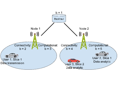
Refer to caption
Figure 1: Example: network slicing in edge computing with autonomous cars.

Example: Let us consider an example where there are two autonomous vehicle service operators, say Slice 111 and Slice 222, coexisting in the same area, and supported by two edge computing nodes equipped with fronthaul connectivity and computational resources (e.g., edge GPUs), as shown in Fig. 1. Both nodes are connected to the same backhaul node. Different resources at different locations are indexed as in the figure. There are 3 vehicles (users) in this area, each of which corresponds to a user class. Users 1 and 2 are on Slice 1, and User 3 is on Slice 2, respectively. Each autonomous vehicle can run either of two applications. User 1 is conducting simple data transmission, with the resource demand vector 𝐝1=(1,1,0,0,0)subscript𝐝111000\mathbf{d}_{1}=(1,1,0,0,0), meaning that User 1’s application involves only connectivity resources, and to achieve a unit transmission rate for User 1, the system needs to allocate all the connectivity resources at both Node 1 and the backhaul. Meanwhile, User 2 and 3 are performing mobile data analytics, with demand vectors 𝐝2=𝐝3=(0.6,0,0,1,1)subscript𝐝2subscript𝐝30.60011\mathbf{d}_{2}=\mathbf{d}_{3}=(0.6,0,0,1,1), meaning that to achieve a unit processing rate for Users 2 or 3, the system needs to allocate 60% of the backhaul resource, all the fronthaul resource, together with all the computational resource at Node 2. Then, for example, if the resource allocation is as given in Table I, the system can achieve user service/processing rates given by λ1=0.4,λ2=λ3=0.5formulae-sequencesubscript𝜆10.4subscript𝜆2subscript𝜆30.5\lambda_{1}=0.4,\lambda_{2}=\lambda_{3}=0.5.

User Resource 1 2 3 4 5 Rate
user 1 0.4 0.4 0 0 0 λ1=0.4subscript𝜆10.4\lambda_{1}=0.4
user 2 0.3 0 0 0.5 0.5 λ2=0.5subscript𝜆20.5\lambda_{2}=0.5
user 3 0.3 0 0 0.5 0.5 λ3=0.5subscript𝜆30.5\lambda_{3}=0.5
TABLE I: Example resource allocation

Next, we introduce the concept of network share. We assign each slice v𝑣v a positive share svsubscript𝑠𝑣s_{v} representing the fraction of overall resources to be committed to slice v𝑣v. The share allocations across slices are denoted by 𝐬:=(sv:v𝒱)\mathbf{s}:=(s_{v}:v\in\mathcal{V}). Without loss of generality we assume v𝒱sv=1subscript𝑣𝒱subscript𝑠𝑣1\sum_{v\in\mathcal{V}}s_{v}=1. In turn, each slice distributes its share svsubscript𝑠𝑣s_{v} across its users u𝒰v𝑢superscript𝒰𝑣u\in\mathcal{U}^{v} according to a Share-constrained weight allocation scheme, defined as follows.

Definition 1.

Share-constrained weight allocation (SCWA): A weight allocation across users 𝐰:=(wu:u𝒰)\mathbf{w}:=(w_{u}:u\in\mathcal{U}) is a share-constrained weight allocation if for each slice v𝑣v,

u𝒰vwu=sv.subscript𝑢superscript𝒰𝑣subscript𝑤𝑢subscript𝑠𝑣\sum_{u\in\mathcal{U}^{v}}w_{u}=s_{v}. (1)

If we consider the weight of each class c𝑐c as qc:=u𝒰cwuassignsubscript𝑞𝑐subscript𝑢subscript𝒰𝑐subscript𝑤𝑢q_{c}:=\sum_{u\in\mathcal{U}_{c}}w_{u}, Eq. (1) implies c𝒞vqc=svsubscript𝑐superscript𝒞𝑣subscript𝑞𝑐subscript𝑠𝑣\sum_{c\in\mathcal{C}^{v}}q_{c}=s_{v}. As a result, a slice can increase its users’ weight by purchasing more shares. Also, note that if the number of users on a slice surges without increasing the associated share, on average each of its users should be given less weight. Two examples of SCWA are

  1. 1.

    equal intra-class weight allocation, where user weights are the same within a user class, i.e., wu=qcncsubscript𝑤𝑢subscript𝑞𝑐subscript𝑛𝑐w_{u}=\frac{q_{c}}{n_{c}}, for u𝒰c𝑢subscript𝒰𝑐u\in\mathcal{U}_{c} with c𝒞vqc=svsubscript𝑐superscript𝒞𝑣subscript𝑞𝑐subscript𝑠𝑣\sum_{c\in\mathcal{C}^{v}}q_{c}=s_{v}; and

  2. 2.

    equal intra-slice weight allocation, where user weights are the same within a slice, i.e., wu=svnvsubscript𝑤𝑢subscript𝑠𝑣superscript𝑛𝑣w_{u}=\frac{s_{v}}{n^{v}}, for u𝒰v𝑢superscript𝒰𝑣u\in\mathcal{U}^{v}. As a result, qc=sv(c)ncnv(c)subscript𝑞𝑐subscript𝑠𝑣𝑐subscript𝑛𝑐superscript𝑛𝑣𝑐q_{c}=\frac{s_{v(c)}n_{c}}{n^{v(c)}}. One can see that equal intra-slice allocation is a further special case of equal intra-class allocation. When each user only demands one resource, such allocation emerges naturally as the social optimal, market and Nash equilibrium when slices exhibit (price taking) strategic behavior in optimizing their own utility, see [8].

In turn, the resources are ultimately committed to users, so a user-level resource allocation criterion is necessary. Let us denote the user rate allocation by 𝝀:=(λu:u𝒰)\bm{\lambda}:=(\lambda_{u}:u\in\mathcal{U}). In this paper, we assume equal intra-class weight allocation is used, resulting in equal rate allocation within a user class. Thus a class-level allocation criterion can be easily converted to a user-level one. For simplicity, the aggregated rate allocation across user classes is then denoted by ϕ=(ϕc:c𝒞)\bm{\phi}=(\phi_{c}:c\in\mathcal{C}), where ϕc:=ncλu,u𝒰cformulae-sequenceassignsubscriptitalic-ϕ𝑐subscript𝑛𝑐subscript𝜆𝑢𝑢subscript𝒰𝑐\phi_{c}:=n_{c}\lambda_{u},u\in\mathcal{U}_{c}, and the weight allocation across user classes by 𝐪=(qc:c𝒞)\mathbf{q}=(q_{c}:c\in\mathcal{C}). For each slice v𝑣v, the weight allocation (across user classes) is 𝐪v:=(qc:c𝒞v)\mathbf{q}^{v}:=(q_{c}:c\in\mathcal{C}^{v}), and the rate allocation is ϕv:=(ϕc:c𝒞v)\bm{\phi}^{v}:=(\phi_{c}:c\in\mathcal{C}^{v}). In view of Eq. (1), we define the normalized weight allocation for slice v𝑣v as 𝐪~v:=(q~c:=qcsv:c𝒞v)\tilde{\mathbf{q}}^{v}:=(\tilde{q}_{c}:=\frac{q_{c}}{s_{v}}:c\in\mathcal{C}^{v}). The rate allocation across slices is 𝜸:=(γv:=c𝒞vϕc:v𝒱)\bm{\gamma}:=(\gamma_{v}:=\sum_{c\in\mathcal{C}^{v}}\phi_{c}:v\in\mathcal{V}). The overall rate across the system is λ:=𝝀1=ϕ1=𝜸1assign𝜆subscriptnorm𝝀1subscriptnormbold-italic-ϕ1subscriptnorm𝜸1\lambda:=\|\bm{\lambda}\|_{1}=\|\bm{\phi}\|_{1}=\|\bm{\gamma}\|_{1}, where 1\|\cdot\|_{1} is the L1-norm. SCS is thus defined as follows.

Definition 2.

αlimit-from𝛼\alpha-Share Constrained Slicing (αlimit-fromα\alpha-SCS): Under equal intra-class weight allocation with class weights 𝐪𝐪\mathbf{q}, a class-level rate allocation ϕbold-ϕ\bm{\phi} corresponds to αlimit-fromα\alpha-SCS if it is the solution to the following problem

maxϕ{Uα(ϕ;𝐪):c𝒞rdcrϕc1,r},subscriptbold-italic-ϕ:subscript𝑈𝛼bold-italic-ϕ𝐪formulae-sequencesubscript𝑐subscript𝒞𝑟subscriptsuperscript𝑑𝑟𝑐subscriptitalic-ϕ𝑐1for-all𝑟\displaystyle\max_{\bm{\phi}}~{}\{U_{\alpha}(\bm{\phi};\mathbf{q}):\sum_{c\in\mathcal{C}_{r}}d^{r}_{c}\phi_{c}\leq 1,\forall r\in\mathcal{R}\}, (2)

where α>0𝛼0\alpha>0 is a pre-defined parameter and

Uα(ϕ;𝐪):={ev𝒱Uαv(ϕv;𝐪v)α=1v𝒱Uαv(ϕv;𝐪v)α>0andα1,assignsubscript𝑈𝛼bold-italic-ϕ𝐪casessuperscript𝑒subscript𝑣𝒱superscriptsubscript𝑈𝛼𝑣superscriptbold-italic-ϕ𝑣superscript𝐪𝑣𝛼1subscript𝑣𝒱superscriptsubscript𝑈𝛼𝑣superscriptbold-italic-ϕ𝑣superscript𝐪𝑣𝛼0and𝛼1\displaystyle U_{\alpha}(\bm{\phi};\mathbf{q}):=\left\{\begin{array}[]{ll}e^{\sum_{v\in\mathcal{V}}U_{\alpha}^{v}(\bm{\phi}^{v};\mathbf{q}^{v})}&\alpha=1\\ \sum_{v\in\mathcal{V}}U_{\alpha}^{v}(\bm{\phi}^{v};\mathbf{q}^{v})&\alpha>0~{}~{}\mbox{and}~{}~{}\alpha\neq 1,\end{array}\right.

where Uαv(ϕv;𝐪v)superscriptsubscript𝑈𝛼𝑣superscriptbold-ϕ𝑣superscript𝐪𝑣U_{\alpha}^{v}(\bm{\phi}^{v};\mathbf{q}^{v}) represents the utility function of slice v𝑣v and is given by

Uαv(ϕv;𝐪v):={c𝒞vqclog(ϕcqc)α=1c𝒞vqc(ϕc/qc)1α1αα>0andα1.assignsuperscriptsubscript𝑈𝛼𝑣superscriptbold-italic-ϕ𝑣superscript𝐪𝑣casessubscript𝑐superscript𝒞𝑣subscript𝑞𝑐subscriptitalic-ϕ𝑐subscript𝑞𝑐𝛼1subscript𝑐superscript𝒞𝑣subscript𝑞𝑐superscriptsubscriptitalic-ϕ𝑐subscript𝑞𝑐1𝛼1𝛼𝛼0and𝛼1\displaystyle U_{\alpha}^{v}(\bm{\phi}^{v};\mathbf{q}^{v}):=\left\{\begin{array}[]{ll}\sum_{c\in\mathcal{C}^{v}}q_{c}\log\left(\frac{\phi_{c}}{q_{c}}\right)&\alpha=1\\ \sum_{c\in\mathcal{C}^{v}}q_{c}\frac{(\phi_{c}/q_{c})^{1-\alpha}}{1-\alpha}&\alpha>0~{}~{}\mbox{and}~{}~{}\alpha\neq 1.\end{array}\right.

The criterion underlying SCS is different from class-level (weighted) αlimit-from𝛼\alpha-fairness proposed in [23] and [4], which is defined as follows.

Definition 3.

Class-level αlimit-from𝛼\alpha-fairness: Under equal intra-class weight allocation, given 𝐪𝐪\mathbf{q}, a class-level rate allocation ϕbold-ϕ\bm{\phi} corresponds to (weighted) αlimit-from𝛼\alpha-fairness if it is the solution to Problem (2) with utility function of slice v𝑣v given by

Uαv(ϕv;𝐪v):={c𝒞vqclog(ϕc)α=1c𝒞vqc(ϕc)1α1αα>0andα1.assignsuperscriptsubscript𝑈𝛼𝑣superscriptbold-italic-ϕ𝑣superscript𝐪𝑣casessubscript𝑐superscript𝒞𝑣subscript𝑞𝑐subscriptitalic-ϕ𝑐𝛼1subscript𝑐superscript𝒞𝑣subscript𝑞𝑐superscriptsubscriptitalic-ϕ𝑐1𝛼1𝛼𝛼0and𝛼1\displaystyle U_{\alpha}^{v}(\bm{\phi}^{v};\mathbf{q}^{v}):=\left\{\begin{array}[]{ll}\sum_{c\in\mathcal{C}^{v}}q_{c}\log\left(\phi_{c}\right)&\alpha=1\\ \sum_{c\in\mathcal{C}^{v}}q_{c}\frac{(\phi_{c})^{1-\alpha}}{1-\alpha}&\alpha>0~{}~{}\mbox{and}~{}~{}\alpha\neq 1.\end{array}\right.

As shown in [23], αlimit-from𝛼\alpha-fairness is equivalent to (weighted) proportional fairness as α=1𝛼1\alpha=1 and unweighted maxmin fairness as α𝛼\alpha\rightarrow\infty, while the asymptotic characterization of αlimit-from𝛼\alpha-SCS is given as follows.

Corollary 1.

αlimit-from𝛼\alpha-SCS is equivalent to (weighted) proportional fairness as α=1𝛼1\alpha=1, and weighted max-min fairness as α𝛼\alpha\rightarrow\infty.

Here under equal intra-class weight allocation, weighted proportional fairness is defined as the solution to the following problem:

maxϕ{c𝒞qclogϕc:c𝒞rdcrϕc1,r},subscriptbold-italic-ϕ:subscript𝑐𝒞subscript𝑞𝑐subscriptitalic-ϕ𝑐formulae-sequencesubscript𝑐subscript𝒞𝑟subscriptsuperscript𝑑𝑟𝑐subscriptitalic-ϕ𝑐1for-all𝑟\displaystyle\max_{\bm{\phi}}~{}\left\{\sum_{c\in\mathcal{C}}q_{c}\log\phi_{c}:\sum_{c\in\mathcal{C}_{r}}d^{r}_{c}\phi_{c}\leq 1,\forall r\in\mathcal{R}\right\}, (6)

and weighted max-min fairness is defined as the solution to the following problem:

maxϕ{minc𝒞ϕcqc:c𝒞rdcrϕc1,r}.subscriptbold-italic-ϕ:subscript𝑐𝒞subscriptitalic-ϕ𝑐subscript𝑞𝑐formulae-sequencesubscript𝑐subscript𝒞𝑟subscriptsuperscript𝑑𝑟𝑐subscriptitalic-ϕ𝑐1for-all𝑟\displaystyle\max_{\bm{\phi}}~{}\left\{\min_{c\in\mathcal{C}}\frac{\phi_{c}}{q_{c}}:\sum_{c\in\mathcal{C}_{r}}d^{r}_{c}\phi_{c}\leq 1,\forall r\in\mathcal{R}\right\}. (7)

The persistence of weight is important, especially when α𝛼\alpha increases. Otherwise, the notion of share does not matter when α𝛼\alpha is large, undermining inter-slice protection. To the best of our knowledge, SCS is the first variation of αlimit-from𝛼\alpha-fairness incorporating user weighting in a consistent manner.

Proof:

When α=1𝛼1\alpha=1, one can see that the maximum is assumed when c𝒞qclog(ϕcqc)subscript𝑐𝒞subscript𝑞𝑐subscriptitalic-ϕ𝑐subscript𝑞𝑐\sum_{c\in\mathcal{C}}q_{c}\log\left(\frac{\phi_{c}}{q_{c}}\right) assumes maximum. Due to the concavity, a rate allocation ϕ:=(ϕc:c𝒞)\bm{\phi}^{*}:=(\phi_{c}^{*}:c\in\mathcal{C}) is the maximizer if and only if

c𝒞qcϕc(ϕcϕc)0,subscript𝑐𝒞subscript𝑞𝑐superscriptsubscriptitalic-ϕ𝑐superscriptsubscriptitalic-ϕ𝑐superscriptsubscriptitalic-ϕ𝑐0\displaystyle\sum_{c\in\mathcal{C}}\frac{q_{c}}{\phi_{c}^{*}}(\phi_{c}^{\prime}-\phi_{c}^{*})\leq 0,

for any feasible ϕsuperscriptbold-italic-ϕ\bm{\phi}^{\prime}. Also, for αlimit-from𝛼\alpha-SCS with weight 𝐪𝐪\mathbf{q}, when α1𝛼1\alpha\neq 1, ϕsuperscriptbold-italic-ϕ\bm{\phi}^{*} is the maximizer if and only if

c𝒞(ϕcqc)α(ϕcϕc)0,subscript𝑐𝒞superscriptsuperscriptsubscriptitalic-ϕ𝑐subscript𝑞𝑐𝛼superscriptsubscriptitalic-ϕ𝑐superscriptsubscriptitalic-ϕ𝑐0\displaystyle\sum_{c\in\mathcal{C}}\left(\frac{\phi_{c}^{*}}{q_{c}}\right)^{-\alpha}(\phi_{c}^{\prime}-\phi_{c}^{*})\leq 0,

for any feasible ϕsuperscriptbold-italic-ϕ\bm{\phi}^{\prime}. One can see that two optimality conditions coincide when α=1𝛼1\alpha=1.

The asymptotic behavior when α𝛼\alpha\rightarrow\infty is a direct corollary of the Lemma 3 in [23]. ∎

Let us define function fα(𝐱;𝐲)subscript𝑓𝛼𝐱𝐲f_{\alpha}(\mathbf{x};\mathbf{y}) of two positive vectors 𝐱,𝐲+n𝐱𝐲subscriptsuperscript𝑛\mathbf{x},\mathbf{y}\in\mathbb{R}^{n}_{+} such that 𝐱1=𝐲1=1subscriptnorm𝐱1subscriptnorm𝐲11\|\mathbf{x}\|_{1}=\|\mathbf{y}\|_{1}=1 as

fα(𝐱;𝐲)={eDKL(𝐱𝐲)α=1(ixi(yixi)1α)1αα>0,α1,subscript𝑓𝛼𝐱𝐲casessuperscript𝑒subscript𝐷𝐾𝐿conditional𝐱𝐲𝛼1superscriptsubscript𝑖subscript𝑥𝑖superscriptsubscript𝑦𝑖subscript𝑥𝑖1𝛼1𝛼formulae-sequence𝛼0𝛼1\displaystyle f_{\alpha}(\mathbf{x};\mathbf{y})=\left\{\begin{array}[]{ll}e^{-D_{KL}(\mathbf{x}\|\mathbf{y})}&\alpha=1\\ \left(\sum_{i}x_{i}\left(\frac{y_{i}}{x_{i}}\right)^{1-\alpha}\right)^{\frac{1}{\alpha}}&\alpha>0,\alpha\neq 1,\end{array}\right. (10)

where DKL()D_{KL}(\cdot\|\cdot) represents the Kulback-Leibler (K-L) divergence. The function fα(𝐱;𝐲)subscript𝑓𝛼𝐱𝐲f_{\alpha}(\mathbf{x};\mathbf{y}) can be viewed as a measure of how close a normalized resource allocation 𝐱𝐱\mathbf{x} is to a normalized weight vector 𝐲𝐲\mathbf{y} in that, for example, when α=1𝛼1\alpha=1, it decreases with the K-L divergence between 𝐱𝐱\mathbf{x} and 𝐲𝐲\mathbf{y}, thus assumes maximum when 𝐱=𝐲𝐱𝐲\mathbf{x}=\mathbf{y}, meaning that the rate allocation is aligned with the specified weights. Thus fα(𝐱;𝐲)subscript𝑓𝛼𝐱𝐲f_{\alpha}(\mathbf{x};\mathbf{y}) can be interpreted as a measure of 𝐲limit-from𝐲\mathbf{y}-weighted fairness of allocation 𝐱𝐱\mathbf{x}.

One can easily show that fα(𝐱;𝐲)subscript𝑓𝛼𝐱𝐲f_{\alpha}(\mathbf{x};\mathbf{y}) is continuous. Moreover, for general α𝛼\alpha and a given 𝐲𝐲\mathbf{y}, the following claim can be shown by setting the partial derivative of the associated Lagrangian to 0.

Proposition 1.

fα(𝐱;𝐲)subscript𝑓𝛼𝐱𝐲f_{\alpha}(\mathbf{x};\mathbf{y}) assumes maximum when the rate is aligned with the weight when no constraint is imposed, i.e.,

fα(𝐲;𝐲)=max𝐱fα(𝐱;𝐲)subscript𝑓𝛼𝐲𝐲subscript𝐱subscript𝑓𝛼𝐱𝐲f_{\alpha}(\mathbf{y};\mathbf{y})=\max_{\mathbf{x}}f_{\alpha}(\mathbf{x};\mathbf{y}) (11)

One can show that for a given α𝛼\alpha, αlimit-from𝛼\alpha-SCS criterion can be factorized as follows.

Proposition 2.

For the αlimit-from𝛼\alpha-SCS criterion,

Uα(ϕ;𝐪)=Eα(λ)(Fαinter(𝜸)Fαintra(ϕ;𝐪))α,subscript𝑈𝛼bold-italic-ϕ𝐪subscript𝐸𝛼𝜆superscriptsubscriptsuperscript𝐹inter𝛼𝜸subscriptsuperscript𝐹intra𝛼bold-italic-ϕ𝐪𝛼U_{\alpha}(\bm{\phi};\mathbf{q})=E_{\alpha}(\lambda)\left(F^{\textrm{inter}}_{\alpha}(\bm{\gamma})F^{\textrm{intra}}_{\alpha}(\bm{\phi};\mathbf{q})\right)^{\alpha}, (12)

where Eα(λ)subscript𝐸𝛼𝜆E_{\alpha}(\lambda), Fαinter(𝛄)subscriptsuperscript𝐹inter𝛼𝛄F^{\textrm{inter}}_{\alpha}(\bm{\gamma}) and Fαintra(ϕ;𝐪)subscriptsuperscript𝐹intra𝛼bold-ϕ𝐪F^{\textrm{intra}}_{\alpha}(\bm{\phi};\mathbf{q}) can be interpreted as the overall network efficiency, inter-slice and intra-slice fairness, respectively.

In Eq. (12), the efficiency is captured by a concave non-decreasing function of λ𝜆\lambda given by

Eα(λ):={λα=1λ1α1αα>0andα1.assignsubscript𝐸𝛼𝜆cases𝜆𝛼1superscript𝜆1𝛼1𝛼𝛼0and𝛼1\displaystyle E_{\alpha}(\lambda):=\left\{\begin{array}[]{ll}\lambda&\alpha=1\\ \frac{\lambda^{1-\alpha}}{1-\alpha}&\alpha>0~{}~{}\mbox{and}~{}~{}\alpha\neq 1.\end{array}\right.

The inter-slice fairness function is given by

Fαinter(𝜸):=fα(𝜸~;𝐬),\displaystyle F^{\textrm{inter}}_{\alpha}(\bm{\gamma}):=f_{\alpha}(\tilde{\bm{\gamma}};\mathbf{s}),

where 𝜸~:=(γ~v:=γv/λ:v𝒱)\tilde{\bm{\gamma}}:=(\tilde{\gamma}^{v}:={\gamma^{v}}/{\lambda}:v\in\mathcal{V}) is the normalized aggregated rate across slices. Let us define the normalized rate allocation across user classes on slice v𝑣v as ϕ~v:=(ϕ~c:=ϕcγv:c𝒞v)\tilde{\bm{\phi}}^{v}:=(\tilde{\phi}_{c}:=\frac{\phi_{c}}{\gamma^{v}}:c\in\mathcal{C}^{v}). The intra-slice fairness term is then given by

Fαintra(ϕ;𝐪):={ev𝒱tαv(𝜸~;𝐬)logfα(ϕ~v;𝐪~v)α=1(v𝒱tαv(𝜸~;𝐬)(fα(ϕ~v;𝐪~v))α)1αα1,assignsubscriptsuperscript𝐹intra𝛼bold-italic-ϕ𝐪casessuperscript𝑒subscript𝑣𝒱subscriptsuperscript𝑡𝑣𝛼~𝜸𝐬subscript𝑓𝛼superscript~bold-italic-ϕ𝑣superscript~𝐪𝑣𝛼1superscriptsubscript𝑣𝒱subscriptsuperscript𝑡𝑣𝛼~𝜸𝐬superscriptsubscript𝑓𝛼superscript~bold-italic-ϕ𝑣superscript~𝐪𝑣𝛼1𝛼𝛼1\displaystyle F^{\textrm{intra}}_{\alpha}(\bm{\phi};\mathbf{q}):=\left\{\begin{array}[]{ll}e^{\sum_{v\in\mathcal{V}}t^{v}_{\alpha}(\tilde{\bm{\gamma}};\mathbf{s})\log f_{\alpha}(\tilde{\bm{\phi}}^{v};\tilde{\mathbf{q}}^{v})}&\alpha=1\\ \left(\sum_{v\in\mathcal{V}}t^{v}_{\alpha}(\tilde{\bm{\gamma}};\mathbf{s})(f_{\alpha}(\tilde{\bm{\phi}}^{v};\tilde{\mathbf{q}}^{v}))^{\alpha}\right)^{\frac{1}{\alpha}}&\alpha\neq 1,\end{array}\right.

where tαv(𝜸~;𝐬)subscriptsuperscript𝑡𝑣𝛼~𝜸𝐬t^{v}_{\alpha}(\tilde{\bm{\gamma}};\mathbf{s}) can be viewed as the weight for the fairness of each slice v𝑣v:

tαv(𝜸~;𝐬):=sv(γ~vsv)1αv𝒱sv(γ~vsv)1α.assignsubscriptsuperscript𝑡𝑣𝛼~𝜸𝐬subscript𝑠𝑣superscriptsuperscript~𝛾𝑣subscript𝑠𝑣1𝛼subscriptsuperscript𝑣𝒱subscript𝑠superscript𝑣superscriptsuperscript~𝛾superscript𝑣subscript𝑠superscript𝑣1𝛼t^{v}_{\alpha}(\tilde{\bm{\gamma}};\mathbf{s}):=\frac{s_{v}(\frac{\tilde{\gamma}^{v}}{s_{v}})^{1-\alpha}}{\sum_{v^{\prime}\in\mathcal{V}}s_{v^{\prime}}(\frac{\tilde{\gamma}^{v^{\prime}}}{s_{v^{\prime}}})^{1-\alpha}}. (15)

One can see that Eq. (12) captures a trade-off among overall network efficiency, inter-slice fairness, which can be seen as a proxy of inter-slice protection, and intra-slice fairness. The significance of fairness increases as α𝛼\alpha increases. When α0𝛼0\alpha\rightarrow 0, αlimit-from𝛼\alpha-SCS is maximizing the overall rate allocated, regardless of the weights. In order to achieve desirable resource utilization, a sharing criterion should realize load-driven elasticity, i.e., the amount of resources provisioned to a user class increases in the number of its users. Under equal intra-slice weight allocation, from Eq. (12) one can observe that, due to the fairness terms, the relative resource allocation of a slice tends to be aligned with 𝐪~v=(ncnv:c𝒞v)\tilde{\mathbf{q}}^{v}=(\frac{n_{c}}{n^{v}}:c\in\mathcal{C}^{v}), i.e., its relative load distribution. Thus the elasticity of αlimit-from𝛼\alpha-SCS is achieved as a result of weighted fairness. Specifically under SCS and parallel resource assumption, i.e., each user only uses one resource, |c|=1,c𝒞formulae-sequencesubscript𝑐1for-all𝑐𝒞|\mathcal{R}_{c}|=1,\forall c\in\mathcal{C}, one can show the following result.

Theorem 1.

Under equal intra-slice weight allocation, assuming |c|=1,c𝒞formulae-sequencesubscript𝑐1for-all𝑐𝒞|\mathcal{R}_{c}|=1,\forall c\in\mathcal{C}, αlimit-from𝛼\alpha-SCS is such that ϕcsubscriptitalic-ϕ𝑐\phi_{c} is a monotonically increasing function of ncsubscript𝑛𝑐n_{c}, when ncsubscript𝑛superscript𝑐n_{c^{\prime}} is fixed for ccsuperscript𝑐𝑐c^{\prime}\neq c.

Specifically in the setting of Theorem 1, each resource r𝑟r will provision its resource across user classes in proportion to sv(c)ncnv(c)subscript𝑠𝑣𝑐subscript𝑛𝑐superscript𝑛𝑣𝑐\frac{s_{v(c)}n_{c}}{n^{v(c)}}.

Such elasticity is key to achieving a sharing scheme that is aware of the inter-slice protection, while still improves the resource utilization by accommodating dynamic user loads on different slices.

III Static Analysis

III-A System model

In this section we will take a closer look at the characterization of SCS slice level rate allocations.

The SCS criterion (Problem (2)) is equivalent to the solution to the following problem

maxϕ{v𝒱Uαv(ϕv;𝐪v):c𝒞rdcrϕc1,r}.subscriptbold-italic-ϕ:subscript𝑣𝒱superscriptsubscript𝑈𝛼𝑣superscriptbold-italic-ϕ𝑣superscript𝐪𝑣formulae-sequencesubscript𝑐subscript𝒞𝑟subscriptsuperscript𝑑𝑟𝑐subscriptitalic-ϕ𝑐1for-all𝑟\displaystyle\max_{\bm{\phi}}~{}\left\{\sum_{v\in\mathcal{V}}U_{\alpha}^{v}(\bm{\phi}^{v};\mathbf{q}^{v}):\sum_{c\in\mathcal{C}_{r}}d^{r}_{c}\phi_{c}\leq 1,~{}~{}\forall r\in\mathcal{R}\right\}. (16)

We shall explore two key desirable properties for a sharing criterion, namely, protection and envyfreeness. In our setting, protection means that no slice is penalized under SCS sharing vs. static partitioning. Envyfreeness means that no slice is motivated to swap its resource allocation with another slice with a smaller share. These two properties together motivate the choice of αlimit-from𝛼\alpha-SCS sharing, and at least partially purchasing a larger share in order to improve performance.

III-B Protection

Formally, let us characterize protection among slices by how much performance deterioration is possible for a slice when switching from static partitioning to αlimit-from𝛼\alpha-SCS sharing. Note that under static partitioning, slices are decoupled, so inter-slice protection is achieved possibly at the cost of efficiency. To be specific, the rate allocation for slice v𝑣v under static partitioning is given by the following problem.

maxϕv{Uαv(ϕv;𝐪v):c𝒞rvdcrϕcsv,r},subscriptsuperscriptbold-italic-ϕ𝑣:superscriptsubscript𝑈𝛼𝑣superscriptbold-italic-ϕ𝑣superscript𝐪𝑣formulae-sequencesubscript𝑐subscriptsuperscript𝒞𝑣𝑟subscriptsuperscript𝑑𝑟𝑐subscriptitalic-ϕ𝑐subscript𝑠𝑣for-all𝑟\displaystyle\max_{\bm{\phi}^{v}}~{}\left\{U_{\alpha}^{v}(\bm{\phi}^{v};\mathbf{q}^{v}):\sum_{c\in\mathcal{C}^{v}_{r}}d^{r}_{c}\phi_{c}\leq s_{v},~{}~{}\forall r\in\mathcal{R}\right\}, (17)

From now on, for a given α𝛼\alpha, let us denote the rate allocation for slice v𝑣v under αlimit-from𝛼\alpha-SCS by ϕv,S:=(ϕcS:c𝒞v)\bm{\phi}^{v,S}:=(\phi^{S}_{c}:c\in\mathcal{C}^{v}), and that under static partitioning by ϕv,P:=(ϕcP:c𝒞v)\bm{\phi}^{v,P}:=(\phi^{P}_{c}:c\in\mathcal{C}^{v}). The parameter α𝛼\alpha is suppressed when there is no ambiguity. The following result demonstrates that αlimit-from𝛼\alpha-SCS with α=1𝛼1\alpha=1 achieves inter-slice protection in that any slice achieves a better utility under αlimit-from𝛼\alpha-SCS sharing.

Theorem 2.

For a given 𝐪𝐪\mathbf{q}, when the resource allocation is performed according to αlimit-from𝛼\alpha-SCS, difference in slice v𝑣v’s utility compared to that under static partitioning is upper-bounded by (when α1𝛼1\alpha\neq 1)

Uvα(ϕv,P;𝐪v)Uvα(ϕv,S;𝐪v)subscriptsuperscript𝑈𝛼𝑣superscriptbold-italic-ϕ𝑣𝑃superscript𝐪𝑣subscriptsuperscript𝑈𝛼𝑣superscriptbold-italic-ϕ𝑣𝑆superscript𝐪𝑣absent\displaystyle U^{\alpha}_{v}(\bm{\phi}^{v,P};\mathbf{q}^{v})-U^{\alpha}_{v}(\bm{\phi}^{v,S};\mathbf{q}^{v})\leq
sv(c𝒞vq~c(rcdcrνr)α1αc𝒞qc(rcdcrνr)α1α),subscript𝑠𝑣subscript𝑐superscript𝒞𝑣subscript~𝑞𝑐superscriptsubscript𝑟subscript𝑐subscriptsuperscript𝑑𝑟𝑐subscriptsuperscript𝜈𝑟𝛼1𝛼subscript𝑐𝒞subscript𝑞𝑐superscriptsubscript𝑟subscript𝑐subscriptsuperscript𝑑𝑟𝑐subscriptsuperscript𝜈𝑟𝛼1𝛼\displaystyle s_{v}\left(\sum_{c\in\mathcal{C}^{v}}\tilde{q}_{c}(\sum_{r\in\mathcal{R}_{c}}d^{r}_{c}\nu^{*}_{r})^{\frac{\alpha-1}{\alpha}}-\sum_{c\in\mathcal{C}}q_{c}(\sum_{r\in\mathcal{R}_{c}}d^{r}_{c}\nu^{*}_{r})^{\frac{\alpha-1}{\alpha}}\right),

where q~c:=qc/sv(c)assignsubscript~𝑞𝑐subscript𝑞𝑐subscript𝑠𝑣𝑐\tilde{q}_{c}:=q_{c}/s_{v(c)} is the normalized weight of class c𝑐c, and νrsubscriptsuperscript𝜈𝑟\nu^{*}_{r} is the optimal dual variable associated with the capacity constraint at resource r𝑟r in Problem (16), also known as the shadow price of resource r𝑟r.

Remark: The right hand side characterizes how the protection changes with α𝛼\alpha. c𝒞vq~c(rcdcrνr)11αsubscript𝑐superscript𝒞𝑣subscript~𝑞𝑐superscriptsubscript𝑟subscript𝑐subscriptsuperscript𝑑𝑟𝑐subscriptsuperscript𝜈𝑟11𝛼\sum_{c\in\mathcal{C}^{v}}\tilde{q}_{c}(\sum_{r\in\mathcal{R}_{c}}d^{r}_{c}\nu^{*}_{r})^{1-\frac{1}{\alpha}} can be viewed as the average of the (11α)limit-from11𝛼(1-\frac{1}{\alpha})-order moment of ‘charged’ resource usage of slice v𝑣v’s user, while c𝒞qc(rcdcrνr)11αsubscript𝑐𝒞subscript𝑞𝑐superscriptsubscript𝑟subscript𝑐subscriptsuperscript𝑑𝑟𝑐subscriptsuperscript𝜈𝑟11𝛼\sum_{c\in\mathcal{C}}q_{c}(\sum_{r\in\mathcal{R}_{c}}d^{r}_{c}\nu^{*}_{r})^{1-\frac{1}{\alpha}} is that of the overall users. When 0<α<10𝛼10<\alpha<1, sharing tends to benefit slices with greater average user usages, at the cost of other slices, while when α>1𝛼1\alpha>1, slices with smaller average user prices are preferred.

When α1𝛼1\alpha\rightarrow 1, the utility of slice v𝑣v, Uvα(ϕv;𝐪v)=11α×c𝒞vqc(ϕcqc)1αsuperscriptsubscript𝑈𝑣𝛼superscriptbold-italic-ϕ𝑣superscript𝐪𝑣11𝛼subscript𝑐superscript𝒞𝑣subscript𝑞𝑐superscriptsubscriptitalic-ϕ𝑐subscript𝑞𝑐1𝛼U_{v}^{\alpha}(\bm{\phi}^{v};\mathbf{q}^{v})=\frac{1}{1-\alpha}\\ \times\sum_{c\in\mathcal{C}^{v}}q_{c}\left(\frac{\phi_{c}}{q_{c}}\right)^{1-\alpha} tends to be non-changing with ϕbold-italic-ϕ\bm{\phi}, so the result in Theorem 2 seems to be trivial. However, due to the factor 11α11𝛼\frac{1}{1-\alpha}, the utility function is not well-defined at α1𝛼1\alpha\rightarrow 1. Thus the exact result for α𝛼\alpha need to be discussed on its own, as in Theorem 3.

Also, note that when SCWA constraint Eq. (1) is voided, another form of the theorem can be written as

Uvα(ϕv,P;𝐪v)Uvα(ϕv,S;𝐪v)wv(pvsvw0wvp¯0),subscriptsuperscript𝑈𝛼𝑣superscriptbold-italic-ϕ𝑣𝑃superscript𝐪𝑣subscriptsuperscript𝑈𝛼𝑣superscriptbold-italic-ϕ𝑣𝑆superscript𝐪𝑣subscript𝑤𝑣subscript𝑝𝑣subscript𝑠𝑣subscript𝑤0subscript𝑤𝑣subscript¯𝑝0U^{\alpha}_{v}(\bm{\phi}^{v,P};\mathbf{q}^{v})-U^{\alpha}_{v}(\bm{\phi}^{v,S};\mathbf{q}^{v})\leq w_{v}(p_{v}-s_{v}\frac{w_{0}}{w_{v}}\bar{p}_{0}),

where wv:=c𝒞vqcassignsubscript𝑤𝑣subscript𝑐superscript𝒞𝑣subscript𝑞𝑐w_{v}:=\sum_{c\in\mathcal{C}^{v}}q_{c} is the total weight of users of slice v𝑣v, w0:=c𝒞qcassignsubscript𝑤0subscript𝑐𝒞subscript𝑞𝑐w_{0}:=\sum_{c\in\mathcal{C}}q_{c} is the total weight of all users, pv:=c𝒞vq~c(rcdcrνr)11αassignsubscript𝑝𝑣subscript𝑐superscript𝒞𝑣subscript~𝑞𝑐superscriptsubscript𝑟subscript𝑐subscriptsuperscript𝑑𝑟𝑐subscriptsuperscript𝜈𝑟11𝛼p_{v}:=\sum_{c\in\mathcal{C}^{v}}\tilde{q}_{c}\left(\sum_{r\in\mathcal{R}_{c}}d^{r}_{c}\nu^{*}_{r}\right)^{1-\frac{1}{\alpha}} is the average 11α11𝛼1-\frac{1}{\alpha} power of the prices of slice v𝑣v’s users, and p¯0:=vwvw0pvassignsubscript¯𝑝0subscript𝑣subscript𝑤𝑣subscript𝑤0subscript𝑝𝑣\bar{p}_{0}:=\sum_{v}\frac{w_{v}}{w_{0}}p_{v} is the weighted average of pvsubscript𝑝𝑣p_{v} across all slices. One could see that, if wvsubscript𝑤𝑣w_{v} is not limited, as wvsubscript𝑤𝑣w_{v}\rightarrow\infty, as long as pvp¯0subscript𝑝𝑣subscript¯𝑝0p_{v}\neq\bar{p}_{0}, the gap can be arbitrarily bad, implying significant utility loss when slice-level sharing is used. In comparison, If we use SCWA, i.e., constrained by Eq. (1), the right hand side equals to sv(pvp¯0)subscript𝑠𝑣subscript𝑝𝑣subscript¯𝑝0s_{v}(p_{v}-\bar{p}_{0}). This quantity is small when svsubscript𝑠𝑣s_{v} is small, or slice v𝑣v’s users do not use many ‘expensive’ resources.

Proof:

Under sharing scheme, the rate allocation for each slice v𝑣v should be the same as the solution to the following problem:

maxϕvsubscriptsuperscriptbold-italic-ϕ𝑣\displaystyle\max_{\bm{\phi}^{v}} Uαv(ϕv;𝐪v)superscriptsubscript𝑈𝛼𝑣superscriptbold-italic-ϕ𝑣superscript𝐪𝑣\displaystyle U_{\alpha}^{v}(\bm{\phi}^{v};\mathbf{q}^{v})
such that c𝒞rvdcrϕcc𝒞rvdcrϕcS,r.formulae-sequencesubscript𝑐subscriptsuperscript𝒞𝑣𝑟subscriptsuperscript𝑑𝑟𝑐subscriptitalic-ϕ𝑐subscript𝑐subscriptsuperscript𝒞𝑣𝑟subscriptsuperscript𝑑𝑟𝑐superscriptsubscriptitalic-ϕ𝑐𝑆for-all𝑟\displaystyle\sum_{c\in\mathcal{C}^{v}_{r}}d^{r}_{c}\phi_{c}\leq\sum_{c\in\mathcal{C}^{v}_{r}}d^{r}_{c}\phi_{c}^{S},~{}~{}\forall r\in\mathcal{R}. (18)

Problem (18) yields solution ϕv,Ssuperscriptbold-italic-ϕ𝑣S\bm{\phi}^{v,\textrm{S}}. In comparison, under static partitioning scheme, the rate allocation for slice v𝑣v is given by

maxϕvsubscriptsuperscriptbold-italic-ϕ𝑣\displaystyle\max_{\bm{\phi}^{v}} Uαv(ϕv;𝐪v)superscriptsubscript𝑈𝛼𝑣superscriptbold-italic-ϕ𝑣superscript𝐪𝑣\displaystyle U_{\alpha}^{v}(\bm{\phi}^{v};\mathbf{q}^{v})
such that c𝒞rvdcrϕcsv,r,formulae-sequencesubscript𝑐subscriptsuperscript𝒞𝑣𝑟subscriptsuperscript𝑑𝑟𝑐subscriptitalic-ϕ𝑐subscript𝑠𝑣for-all𝑟\displaystyle\sum_{c\in\mathcal{C}^{v}_{r}}d^{r}_{c}\phi_{c}\leq s_{v},~{}~{}\forall r\in\mathcal{R}, (19)

which can be regarded as a perturbed version of Problem (18), and yields solution ϕv,Psuperscriptbold-italic-ϕ𝑣P\bm{\phi}^{v,\textrm{P}}. It is a well known result in convex optimization [7] that the change in the optimal objective function value due to perturbation of the constraints can be bounded by:

Uvα(ϕv,P;𝐪v)Uvα(ϕv,S;𝐪v)rνr(c𝒞rvdcrϕcSsv).subscriptsuperscript𝑈𝛼𝑣superscriptbold-italic-ϕ𝑣Psuperscript𝐪𝑣subscriptsuperscript𝑈𝛼𝑣superscriptbold-italic-ϕ𝑣Ssuperscript𝐪𝑣subscript𝑟subscriptsuperscript𝜈𝑟subscript𝑐subscriptsuperscript𝒞𝑣𝑟subscriptsuperscript𝑑𝑟𝑐superscriptsubscriptitalic-ϕ𝑐𝑆subscript𝑠𝑣U^{\alpha}_{v}(\bm{\phi}^{v,\textrm{P}};\mathbf{q}^{v})-U^{\alpha}_{v}(\bm{\phi}^{v,\textrm{S}};\mathbf{q}^{v})\leq\sum_{r\in\mathcal{R}}\nu^{*}_{r}\left(\sum_{c\in\mathcal{C}^{v}_{r}}d^{r}_{c}\phi_{c}^{S}-s_{v}\right). (20)

The Lagrangian of Problem (18) is

Lα(ϕv;𝝂)=11αc𝒞vqc(ϕcqc)1αsuperscript𝐿𝛼superscriptbold-italic-ϕ𝑣𝝂11𝛼subscript𝑐superscript𝒞𝑣subscript𝑞𝑐superscriptsubscriptitalic-ϕ𝑐subscript𝑞𝑐1𝛼\displaystyle L^{\alpha}(\bm{\phi}^{v};\bm{\nu})=-\frac{1}{1-\alpha}\sum_{c\in\mathcal{C}^{v}}q_{c}\left(\frac{\phi_{c}}{q_{c}}\right)^{1-\alpha} (21)
+rνr(c𝒞rvdcrϕcc𝒞rvdcrϕcS).subscript𝑟subscript𝜈𝑟subscript𝑐subscriptsuperscript𝒞𝑣𝑟subscriptsuperscript𝑑𝑟𝑐subscriptitalic-ϕ𝑐subscript𝑐subscriptsuperscript𝒞𝑣𝑟subscriptsuperscript𝑑𝑟𝑐superscriptsubscriptitalic-ϕ𝑐𝑆\displaystyle+\sum_{r\in\mathcal{R}}\nu_{r}(\sum_{c\in\mathcal{C}^{v}_{r}}d^{r}_{c}\phi_{c}-\sum_{c\in\mathcal{C}^{v}_{r}}d^{r}_{c}\phi_{c}^{S}).

Setting the partial derivative against ϕvsuperscriptbold-italic-ϕ𝑣\bm{\phi}^{v} to 0, we obtain the dual function as:

gα(𝝂)=11αc𝒞vqc(rcdcrνr)11αsuperscript𝑔𝛼𝝂11𝛼subscript𝑐superscript𝒞𝑣subscript𝑞𝑐superscriptsubscript𝑟subscript𝑐subscriptsuperscript𝑑𝑟𝑐subscript𝜈𝑟11𝛼\displaystyle g^{\alpha}(\bm{\nu})=-\frac{1}{1-\alpha}\sum_{c\in\mathcal{C}^{v}}q_{c}\left(\sum_{r\in\mathcal{R}_{c}}d^{r}_{c}\nu_{r}\right)^{1-\frac{1}{\alpha}}
+rνr(c𝒞rvdcrqc(rcdcrνr)1αc𝒞rvdcrϕcS).subscript𝑟subscript𝜈𝑟subscript𝑐subscriptsuperscript𝒞𝑣𝑟subscriptsuperscript𝑑𝑟𝑐subscript𝑞𝑐superscriptsubscriptsuperscript𝑟subscript𝑐subscriptsuperscript𝑑superscript𝑟𝑐subscript𝜈superscript𝑟1𝛼subscript𝑐subscriptsuperscript𝒞𝑣𝑟subscriptsuperscript𝑑𝑟𝑐superscriptsubscriptitalic-ϕ𝑐𝑆\displaystyle+\sum_{r\in\mathcal{R}}\nu_{r}\left(\sum_{c\in\mathcal{C}^{v}_{r}}d^{r}_{c}q_{c}\left(\sum_{r^{\prime}\in\mathcal{R}_{c}}d^{r^{\prime}}_{c}\nu_{r^{\prime}}\right)^{-\frac{1}{\alpha}}-\sum_{c\in\mathcal{C}^{v}_{r}}d^{r}_{c}\phi_{c}^{S}\right).

Also,

ϕcS=qc(rcdcrνr)1α.superscriptsubscriptitalic-ϕ𝑐𝑆subscript𝑞𝑐superscriptsubscriptsuperscript𝑟subscript𝑐subscriptsuperscript𝑑superscript𝑟𝑐subscriptsuperscript𝜈superscript𝑟1𝛼\phi_{c}^{S}=q_{c}\left(\sum_{r^{\prime}\in\mathcal{R}_{c}}d^{r^{\prime}}_{c}\nu^{*}_{r^{\prime}}\right)^{-\frac{1}{\alpha}}. (22)

By swapping the order of summation, one can show that

rνrc𝒞rvdcrqc(rcdcrνr)1α=subscript𝑟subscript𝜈𝑟subscript𝑐subscriptsuperscript𝒞𝑣𝑟subscriptsuperscript𝑑𝑟𝑐subscript𝑞𝑐superscriptsubscriptsuperscript𝑟subscript𝑐subscriptsuperscript𝑑superscript𝑟𝑐subscript𝜈superscript𝑟1𝛼absent\displaystyle\sum_{r\in\mathcal{R}}\nu_{r}\sum_{c\in\mathcal{C}^{v}_{r}}d^{r}_{c}q_{c}\left(\sum_{r^{\prime}\in\mathcal{R}_{c}}d^{r^{\prime}}_{c}\nu_{r^{\prime}}\right)^{-\frac{1}{\alpha}}=
c𝒞vqc(rcdcrνr)11α.subscript𝑐superscript𝒞𝑣subscript𝑞𝑐superscriptsubscript𝑟subscript𝑐subscriptsuperscript𝑑𝑟𝑐subscript𝜈𝑟11𝛼\displaystyle\sum_{c\in\mathcal{C}^{v}}q_{c}\left(\sum_{r\in\mathcal{R}_{c}}d^{r}_{c}\nu_{r}\right)^{1-\frac{1}{\alpha}}.

Due to strong convexity of Problem (18), we know

gα(𝝂)=11αc𝒞vqc(ϕcSqc)1α.superscript𝑔𝛼superscript𝝂11𝛼subscript𝑐superscript𝒞𝑣subscript𝑞𝑐superscriptsuperscriptsubscriptitalic-ϕ𝑐𝑆subscript𝑞𝑐1𝛼g^{\alpha}(\bm{\nu}^{*})=-\frac{1}{1-\alpha}\sum_{c\in\mathcal{C}^{v}}q_{c}\left(\frac{\phi_{c}^{S}}{q_{c}}\right)^{1-\alpha}.

Plugging in Eq. (22) we have

c𝒞vqc(rcdcrνr)11αrνrc𝒞rvdcrϕcS=0.subscript𝑐superscript𝒞𝑣subscript𝑞𝑐superscriptsubscript𝑟subscript𝑐subscriptsuperscript𝑑𝑟𝑐superscriptsubscript𝜈𝑟11𝛼subscript𝑟subscriptsuperscript𝜈𝑟subscript𝑐subscriptsuperscript𝒞𝑣𝑟subscriptsuperscript𝑑𝑟𝑐superscriptsubscriptitalic-ϕ𝑐𝑆0\sum_{c\in\mathcal{C}^{v}}q_{c}\left(\sum_{r\in\mathcal{R}_{c}}d^{r}_{c}\nu_{r}^{*}\right)^{1-\frac{1}{\alpha}}-\sum_{r\in\mathcal{R}}\nu^{*}_{r}\sum_{c\in\mathcal{C}^{v}_{r}}d^{r}_{c}\phi_{c}^{S}=0. (23)

Note that if a resource is binding, the sum of resource allocated should equal to 1. Otherwise it has 0 shadow price. Summing above across v𝒱𝑣𝒱v\in\mathcal{V}, we have

c𝒞qc(rcdcrνr)11αrνr=0.subscript𝑐𝒞subscript𝑞𝑐superscriptsubscript𝑟subscript𝑐subscriptsuperscript𝑑𝑟𝑐superscriptsubscript𝜈𝑟11𝛼subscript𝑟superscriptsubscript𝜈𝑟0\sum_{c\in\mathcal{C}}q_{c}\left(\sum_{r\in\mathcal{R}_{c}}d^{r}_{c}\nu_{r}^{*}\right)^{1-\frac{1}{\alpha}}-\sum_{r\in\mathcal{R}}\nu_{r}^{*}=0. (24)

Plugging in the right hand side of Eq. (20) to substitute rνrsubscript𝑟superscriptsubscript𝜈𝑟\sum_{r\in\mathcal{R}}\nu_{r}^{*}, and also plugging in Eq. (22), the theorem is proved. ∎

Following is the result specifically for the case when α=1𝛼1\alpha=1.

Theorem 3.

For a given 𝐪𝐪\mathbf{q}, when the resource allocation is performed according to 1limit-from11-SCS, slice v𝑣v’s utility exceeds that under static partitioning (Problem (17)), i.e.,

U1v(ϕv,P;𝐪v)U1v(ϕv,S;𝐪v).subscriptsuperscript𝑈𝑣1superscriptbold-italic-ϕ𝑣𝑃superscript𝐪𝑣subscriptsuperscript𝑈𝑣1superscriptbold-italic-ϕ𝑣𝑆superscript𝐪𝑣U^{v}_{1}(\bm{\phi}^{v,P};\mathbf{q}^{v})\leq U^{v}_{1}(\bm{\phi}^{v,S};\mathbf{q}^{v}). (25)

Remark: It is a straightforward observation that under αlimit-from𝛼\alpha-SCS, the global utility v𝒱U1v(ϕv;𝐪v)subscript𝑣𝒱subscriptsuperscript𝑈𝑣1superscriptbold-italic-ϕ𝑣superscript𝐪𝑣\sum_{v\in\mathcal{V}}U^{v}_{1}(\bm{\phi}^{v};\mathbf{q}^{v}) is improved since it can be viewed as relaxing the system constraints. However, Theorem 3 asserts that this holds uniformly on a per slice basis.

Proof:

Similar to the argument for general α𝛼\alpha, we have that the gap between sharing and static partitioning satisfies Eq. (20). Also, by solving the first order condition, one can obtain that ϕcS=qcrcdcrνrsubscriptsuperscriptitalic-ϕ𝑆𝑐subscript𝑞𝑐subscript𝑟subscript𝑐subscriptsuperscript𝑑𝑟𝑐superscriptsubscript𝜈𝑟\phi^{S}_{c}=\frac{q_{c}}{\sum_{r\in\mathcal{R}_{c}}d^{r}_{c}\nu_{r}^{*}}. By plugging in this expression and swapping the order of summation we have

U1v(ϕv,P;𝐪v)U1v(ϕv,S;𝐪v)sv(1rνr),subscriptsuperscript𝑈𝑣1superscriptbold-italic-ϕ𝑣𝑃superscript𝐪𝑣subscriptsuperscript𝑈𝑣1superscriptbold-italic-ϕ𝑣𝑆superscript𝐪𝑣subscript𝑠𝑣1subscript𝑟superscriptsubscript𝜈𝑟U^{v}_{1}(\bm{\phi}^{v,P};\mathbf{q}^{v})-U^{v}_{1}(\bm{\phi}^{v,S};\mathbf{q}^{v})\leq s_{v}(1-\sum_{r\in\mathcal{R}}\nu_{r}^{*}), (26)

where νrsuperscriptsubscript𝜈𝑟\nu_{r}^{*} is the shadow price of resource r𝑟r under SCS, or the dual variables associated with the capacity constraints.

Then if we have rνr=1subscript𝑟superscriptsubscript𝜈𝑟1\sum_{r\in\mathcal{R}}\nu_{r}^{*}=1, the proof is complete. For α=1𝛼1\alpha=1, the Lagrangian is given by

L1(ϕv;𝝂)=c𝒞vqclogϕc+rνr(c𝒞rvdcrϕcc𝒞rvdcrϕcS).superscript𝐿1superscriptbold-italic-ϕ𝑣𝝂subscript𝑐superscript𝒞𝑣subscript𝑞𝑐subscriptitalic-ϕ𝑐subscript𝑟subscript𝜈𝑟subscript𝑐subscriptsuperscript𝒞𝑣𝑟subscriptsuperscript𝑑𝑟𝑐subscriptitalic-ϕ𝑐subscript𝑐subscriptsuperscript𝒞𝑣𝑟subscriptsuperscript𝑑𝑟𝑐superscriptsubscriptitalic-ϕ𝑐𝑆L^{1}(\bm{\phi}^{v};\bm{\nu})=-\sum_{c\in\mathcal{C}^{v}}q_{c}\log\phi_{c}+\sum_{r\in\mathcal{R}}\nu_{r}(\sum_{c\in\mathcal{C}^{v}_{r}}d^{r}_{c}\phi_{c}-\sum_{c\in\mathcal{C}^{v}_{r}}d^{r}_{c}\phi_{c}^{S}).

By setting the derivative against ϕvsuperscriptbold-italic-ϕ𝑣\bm{\phi}^{v} to 0, we have the dual function as

g1(𝝂)=c𝒞vqclogqcrcdcrνr+svrνrc𝒞rvdcrϕcS,superscript𝑔1𝝂subscript𝑐superscript𝒞𝑣subscript𝑞𝑐subscript𝑞𝑐subscript𝑟subscript𝑐subscriptsuperscript𝑑𝑟𝑐subscript𝜈𝑟subscript𝑠𝑣subscript𝑟subscript𝜈𝑟subscript𝑐subscriptsuperscript𝒞𝑣𝑟subscriptsuperscript𝑑𝑟𝑐superscriptsubscriptitalic-ϕ𝑐𝑆g^{1}(\bm{\nu})=-\sum_{c\in\mathcal{C}^{v}}q_{c}\log\frac{q_{c}}{\sum_{r\in\mathcal{R}_{c}}d^{r}_{c}\nu_{r}}+s_{v}-\sum_{r\in\mathcal{R}}\nu_{r}\sum_{c\in\mathcal{C}^{v}_{r}}d^{r}_{c}\phi_{c}^{S},

and

ϕcS=qcrcdcrνr.superscriptsubscriptitalic-ϕ𝑐𝑆subscript𝑞𝑐subscript𝑟subscript𝑐subscriptsuperscript𝑑𝑟𝑐subscriptsuperscript𝜈𝑟\phi_{c}^{S}=\frac{q_{c}}{\sum_{r\in\mathcal{R}_{c}}d^{r}_{c}\nu^{*}_{r}}. (27)

By strong duality, maximal dual should be minimal primal function. And optimal dual is achieved at the shadow price 𝝂superscript𝝂\bm{\nu}^{*}. Thus,

g1(𝝂)=c𝒞vqclogϕcS,superscript𝑔1superscript𝝂subscript𝑐superscript𝒞𝑣subscript𝑞𝑐superscriptsubscriptitalic-ϕ𝑐𝑆g^{1}(\bm{\nu}^{*})=-\sum_{c\in\mathcal{C}^{v}}q_{c}\log\phi_{c}^{S},

which gives us

svrνrc𝒞rvdcrϕcS=0.subscript𝑠𝑣subscript𝑟subscriptsuperscript𝜈𝑟subscript𝑐subscriptsuperscript𝒞𝑣𝑟subscriptsuperscript𝑑𝑟𝑐superscriptsubscriptitalic-ϕ𝑐𝑆0s_{v}-\sum_{r\in\mathcal{R}}\nu^{*}_{r}\sum_{c\in\mathcal{C}^{v}_{r}}d^{r}_{c}\phi_{c}^{S}=0. (28)

Summing above across v𝒱𝑣𝒱v\in\mathcal{V} we have 1rνr=01subscript𝑟subscriptsuperscript𝜈𝑟01-\sum_{r\in\mathcal{R}}\nu^{*}_{r}=0. Because if a resource is binding, the sum of rate allocated should be equal to 1. Otherwise it has 0 shadow price. Plugging above result into Eq. (26), the theorem is proved. ∎

III-C Envyfreeness

Formally, envyfreeness is defined under the assumption that, for two slices v𝑣v and vsuperscript𝑣v^{\prime}, if they swap their allocated resources, slice v𝑣v’s associated utility will not be improved if svsvsubscript𝑠superscript𝑣subscript𝑠𝑣s_{v^{\prime}}\leq s_{v}. Before swapping, the rate allocation for slice v𝑣v is given by ϕv,Ssuperscriptbold-italic-ϕ𝑣𝑆\bm{\phi}^{v,S}, while after swapping with slice vsuperscript𝑣v^{\prime}, its rate allocation is determined by solving following problem:

maxϕv{Uαv(ϕv;𝐪v):c𝒞rvdcrϕcc𝒞rvdcrϕcS,r}.subscriptsuperscriptbold-italic-ϕ𝑣:subscriptsuperscript𝑈𝑣𝛼superscriptbold-italic-ϕ𝑣superscript𝐪𝑣formulae-sequencesubscript𝑐subscriptsuperscript𝒞𝑣𝑟subscriptsuperscript𝑑𝑟𝑐subscriptitalic-ϕ𝑐subscript𝑐subscriptsuperscript𝒞superscript𝑣𝑟subscriptsuperscript𝑑𝑟𝑐superscriptsubscriptitalic-ϕ𝑐𝑆for-all𝑟\displaystyle\max_{\bm{\phi}^{v}}~{}\{U^{v}_{\alpha}(\bm{\phi}^{v};\mathbf{q}^{v}):\sum_{c\in\mathcal{C}^{v}_{r}}d^{r}_{c}\phi_{c}\leq\sum_{c\in\mathcal{C}^{v^{\prime}}_{r}}d^{r}_{c}\phi_{c}^{S},~{}\forall r\in\mathcal{R}\}.

Note that c𝒞rvdcrϕcSsubscript𝑐subscriptsuperscript𝒞superscript𝑣𝑟subscriptsuperscript𝑑𝑟𝑐superscriptsubscriptitalic-ϕ𝑐𝑆\sum_{c\in\mathcal{C}^{v^{\prime}}_{r}}d^{r}_{c}\phi_{c}^{S} corresponds to the fraction of resource r𝑟r provisioned to slice vsuperscript𝑣v^{\prime}. Let us denote the solution to such problem for slice v𝑣v as ϕvvsuperscriptbold-italic-ϕ𝑣superscript𝑣\bm{\phi}^{v\leftrightarrow v^{\prime}}. Then we have following result.

Theorem 4.

The difference between the utility obtained by slice v𝑣v under αlimit-from𝛼\alpha-SCS with SCWA, and that under static partitioning within the resource provisioned to another slice vsuperscript𝑣v^{\prime} is upper-bounded by the following inequality:

Uαv(ϕvv;𝐪v)Uαv(ϕv,S;𝐪v)subscriptsuperscript𝑈𝑣𝛼superscriptbold-italic-ϕ𝑣superscript𝑣superscript𝐪𝑣subscriptsuperscript𝑈𝑣𝛼superscriptbold-italic-ϕ𝑣𝑆superscript𝐪𝑣absent\displaystyle U^{v}_{\alpha}(\bm{\phi}^{v\leftrightarrow v^{\prime}};\mathbf{q}^{v})-U^{v}_{\alpha}(\bm{\phi}^{v,S};\mathbf{q}^{v})\leq
c𝒞vqc(rcdcrνr)α1αc𝒞vqc(rcdcrνr)α1α.subscript𝑐superscript𝒞superscript𝑣subscript𝑞𝑐superscriptsubscript𝑟subscript𝑐subscriptsuperscript𝑑𝑟𝑐subscriptsuperscript𝜈𝑟𝛼1𝛼subscript𝑐superscript𝒞𝑣subscript𝑞𝑐superscriptsubscript𝑟subscript𝑐subscriptsuperscript𝑑𝑟𝑐subscriptsuperscript𝜈𝑟𝛼1𝛼\displaystyle\sum_{c\in\mathcal{C}^{v^{\prime}}}q_{c}\left(\sum_{r\in\mathcal{R}_{c}}d^{r}_{c}\nu^{*}_{r}\right)^{\frac{\alpha-1}{\alpha}}-\sum_{c\in\mathcal{C}^{v}}q_{c}\left(\sum_{r\in\mathcal{R}_{c}}d^{r}_{c}\nu^{*}_{r}\right)^{\frac{\alpha-1}{\alpha}}.

Remark: As a special case, when α=1𝛼1\alpha=1, the right hand side of the inequality becomes svsvsubscript𝑠superscript𝑣subscript𝑠𝑣s_{v^{\prime}}-s_{v}, and thus a slice has no incentive to swap its allocation with another with a less or equal share, which implies SCS is envyfree. Envyfreeness implies that αlimit-from𝛼\alpha-SCS achieves desirable resource utilization in that the right portion of resource is provisioned to the right slice.

Proof:

Still by the sensitivity of convex optimization problem [7], we have

Uαv(𝝀vv;𝐪v)Uαv(𝝀v,S;𝐪v)subscriptsuperscript𝑈𝑣𝛼superscript𝝀𝑣superscript𝑣superscript𝐪𝑣subscriptsuperscript𝑈𝑣𝛼superscript𝝀𝑣𝑆superscript𝐪𝑣absent\displaystyle U^{v}_{\alpha}(\bm{\lambda}^{v\leftrightarrow v^{\prime}};\mathbf{q}^{v})-U^{v}_{\alpha}(\bm{\lambda}^{v,S};\mathbf{q}^{v})\leq (29)
rνr(c𝒞rvdcrϕcSc𝒞rvdcrϕcS).subscript𝑟subscriptsuperscript𝜈𝑟subscript𝑐subscriptsuperscript𝒞superscript𝑣𝑟subscriptsuperscript𝑑𝑟𝑐subscriptsuperscriptitalic-ϕ𝑆𝑐subscript𝑐subscriptsuperscript𝒞𝑣𝑟subscriptsuperscript𝑑𝑟𝑐subscriptsuperscriptitalic-ϕ𝑆𝑐\displaystyle\sum_{r\in\mathcal{R}}\nu^{*}_{r}\left(\sum_{c\in\mathcal{C}^{v^{\prime}}_{r}}d^{r}_{c}\phi^{S}_{c}-\sum_{c\in\mathcal{C}^{v}_{r}}d^{r}_{c}\phi^{S}_{c}\right).

Then by substituting Eq. (23) the theorem is proved. ∎

III-D Using limit-from\infty-SCS as a surrogate for 1limit-from11-SCS

From previous discussions, one can see that it is of particular interest to use 1limit-from11-SCS as the fairness criterion, for it achieves strict protection and envyfreeness. When α=1𝛼1\alpha=1, αlimit-from𝛼\alpha-SCS becomes weighted proportional fairness, whose solution usually involves iterative methods, and the complexity increases rapidly with the number of user classes as well as the accuracy requirement, see, e.g., [26], making it hard to implement in large-scale. In comparison, weighted max-min is relatively easy to implement in distributed manner, see [20] for example. Specifically a progressive water-filling algorithm [26] has O(|𝒞|maxc𝒞|c|)𝑂𝒞subscript𝑐𝒞subscript𝑐O(|\mathcal{C}|\max_{c\in\mathcal{C}}|\mathcal{R}_{c}|) complexity. Thus, in our work we will discuss the feasibility of using limit-from\infty-SCS, which is equivalent to a (dynamically) weighted maxmin, as a surrogate to 1limit-from11-SCS. If the resulted utility function is not far from the optimum of 1limit-from11-SCS criterion, we shall assert limit-from\infty-SCS achieves similar performance as 1limit-from11-SCS.

For simplicity, we consider the original form of weighted-log utility, given by

Ψ(ϕ;𝐪):=c𝒞qclogϕc.assignΨbold-italic-ϕ𝐪subscript𝑐𝒞subscript𝑞𝑐subscriptitalic-ϕ𝑐\Psi(\bm{\phi};\mathbf{q}):=\sum_{c\in\mathcal{C}}q_{c}\log\phi_{c}. (30)

Then for the overall utility achieved, we have following theorem.

Theorem 5.

For a given weight allocation 𝐪𝐪\mathbf{q}, if dcr1,r,c𝒞formulae-sequencesubscriptsuperscript𝑑𝑟𝑐1formulae-sequencefor-all𝑟𝑐𝒞d^{r}_{c}\geq 1,\forall r\in\mathcal{R},c\in\mathcal{C}, we have

Ψ(ϕ,1;𝐪)Ψ(ϕ,;𝐪)c𝒞qcDc1,Ψsuperscriptbold-italic-ϕ1𝐪Ψsuperscriptbold-italic-ϕ𝐪subscript𝑐𝒞subscript𝑞𝑐subscript𝐷𝑐1\Psi(\bm{\phi}^{*,1};\mathbf{q})-\Psi(\bm{\phi}^{*,\infty};\mathbf{q})\leq\sum_{c\in\mathcal{C}}q_{c}D_{c}-1, (31)

where ϕ,α:=(ϕc,α:c𝒞)\bm{\phi}^{*,\alpha}:=(\phi^{*,\alpha}_{c}:c\in\mathcal{C}) is the optimal rate allocation under αlimit-from𝛼\alpha-SCS, and Dc:=rcdcrassignsubscript𝐷𝑐subscript𝑟subscript𝑐subscriptsuperscript𝑑𝑟𝑐D_{c}:=\sum_{r\in\mathcal{R}_{c}}d^{r}_{c}.

Remark: First note that the condition dcr1subscriptsuperscript𝑑𝑟𝑐1d^{r}_{c}\geq 1 can be easily satisfied by rescaling the unit of rate without loss of generality. Also by rescaling, one can show that such bound vanishes when each user class is associated with only one resource, i.e., |c|=1,c𝒞formulae-sequencesubscript𝑐1for-all𝑐𝒞|\mathcal{R}_{c}|=1,\forall c\in\mathcal{C}, and dcrsubscriptsuperscript𝑑𝑟𝑐d^{r}_{c} are the same, e.g., dcr=1subscriptsuperscript𝑑𝑟𝑐1d^{r}_{c}=1. Such bound implies that, the suboptimality due to using a surrogate solution to achieve weighted proportional fairness depends on the diversity in the users’ requirements on resources. Also, this gap of suboptimality cannot be arbitrarily bad because under SCWA, we have cqc=1subscript𝑐subscript𝑞𝑐1\sum_{c}q_{c}=1, thus the right hand side of Eq. (31) is at most maxcDc1subscript𝑐subscript𝐷𝑐1\max_{c}D_{c}-1.

Proof:

Note that when α𝛼\alpha\rightarrow\infty, SCS approaches weighted maxmin, which can be solved by a progressive water-filling algorithm. Let us denote the resource where class c𝑐c is bottlenecked under weighted maxmin by r(c)𝑟𝑐r(c), and in turn, the set of users being bottlenecked at resource r𝑟r by 𝒞~rsubscript~𝒞𝑟\tilde{\mathcal{C}}_{r} . Let us define νrsubscriptsuperscript𝜈𝑟\nu^{*}_{r} as the shadow price for resource r𝑟r when α=1𝛼1\alpha=1. According to the definition we have

Ψ(ϕ,1;𝐪)Ψ(ϕ,;𝐪)Ψsuperscriptbold-italic-ϕ1𝐪Ψsuperscriptbold-italic-ϕ𝐪\displaystyle\Psi(\bm{\phi}^{*,1};\mathbf{q})-\Psi(\bm{\phi}^{*,\infty};\mathbf{q})
=\displaystyle= cqc(logϕc,1logϕc,)subscript𝑐subscript𝑞𝑐superscriptsubscriptitalic-ϕ𝑐1superscriptsubscriptitalic-ϕ𝑐\displaystyle\sum_{c}q_{c}(\log\phi_{c}^{*,1}-\log\phi_{c}^{*,\infty})
\displaystyle\leq cqc(logqcrcdcrνr\displaystyle\sum_{c}q_{c}\left(\log\frac{q_{c}}{\sum_{r^{\prime}\in\mathcal{R}_{c}}d_{c}^{r^{\prime}}\nu_{r^{\prime}}^{*}}\right.
log(qcc𝒞r(c)dcr(c)qc))\displaystyle-\left.\log\left(\frac{q_{c}}{\sum_{c^{\prime}\in\mathcal{C}_{r(c)}}d_{c^{\prime}}^{r(c)}q_{c^{\prime}}}\right)\right)
=\displaystyle= rc𝒞~rqclog(c𝒞rdcrqcrcdcrνr).subscript𝑟subscript𝑐subscript~𝒞𝑟subscript𝑞𝑐subscriptsuperscript𝑐subscript𝒞𝑟superscriptsubscript𝑑superscript𝑐𝑟subscript𝑞superscript𝑐subscriptsuperscript𝑟subscript𝑐superscriptsubscript𝑑𝑐superscript𝑟superscriptsubscript𝜈superscript𝑟\displaystyle\sum_{r\in\mathcal{R}}\sum_{c\in\tilde{\mathcal{C}}_{r}}q_{c}\log\left(\frac{\sum_{c^{\prime}\in\mathcal{C}_{r}}d_{c^{\prime}}^{r}q_{c^{\prime}}}{\sum_{r^{\prime}\in\mathcal{R}_{c}}d_{c}^{r^{\prime}}\nu_{r^{\prime}}^{*}}\right).

The first inequality follows from the form of solution of sharing problem when α=1𝛼1\alpha=1, and the fact that ϕc,qcc𝒞r(c)dcr(c)qcsuperscriptsubscriptitalic-ϕ𝑐subscript𝑞𝑐subscriptsuperscript𝑐subscript𝒞𝑟𝑐superscriptsubscript𝑑superscript𝑐𝑟𝑐subscript𝑞superscript𝑐\phi_{c}^{*,\infty}\geq\frac{q_{c}}{\sum_{c^{\prime}\in\mathcal{C}_{r(c)}}d_{c^{\prime}}^{r(c)}q_{c^{\prime}}}, since the worst rate user u𝑢u could obtain is when there is no other users get saturated before it at its bottleneck resource. Because logxx1𝑥𝑥1\log x\leq x-1 we have

Ψ(ϕ,1;𝐪)Ψ(𝝀,;𝐪)Ψsuperscriptbold-italic-ϕ1𝐪Ψsuperscript𝝀𝐪\displaystyle\Psi(\bm{\phi}^{*,1};\mathbf{q})-\Psi(\bm{\lambda}^{*,\infty};\mathbf{q})
\displaystyle\leq rc𝒞~rqcc𝒞rdcrqcrcdcrνr1subscript𝑟subscript𝑐subscript~𝒞𝑟subscript𝑞𝑐subscriptsuperscript𝑐subscript𝒞𝑟superscriptsubscript𝑑superscript𝑐𝑟subscript𝑞superscript𝑐subscriptsuperscript𝑟subscript𝑐superscriptsubscript𝑑𝑐superscript𝑟superscriptsubscript𝜈superscript𝑟1\displaystyle\sum_{r\in\mathcal{R}}\sum_{c\in\tilde{\mathcal{C}}_{r}}q_{c}\frac{\sum_{c^{\prime}\in\mathcal{C}_{r}}d_{c^{\prime}}^{r}q_{c^{\prime}}}{\sum_{r^{\prime}\in\mathcal{R}_{c}}d_{c}^{r^{\prime}}\nu_{r^{\prime}}^{*}}-1
=\displaystyle= r(c𝒞rdcrqc)c𝒞~rqcrcdcrνr1subscript𝑟subscriptsuperscript𝑐subscript𝒞𝑟superscriptsubscript𝑑superscript𝑐𝑟subscript𝑞superscript𝑐subscript𝑐subscript~𝒞𝑟subscript𝑞𝑐subscriptsuperscript𝑟subscript𝑐superscriptsubscript𝑑𝑐superscript𝑟superscriptsubscript𝜈superscript𝑟1\displaystyle\sum_{r\in\mathcal{R}}\left(\sum_{c^{\prime}\in\mathcal{C}_{r}}d_{c^{\prime}}^{r}q_{c^{\prime}}\right)\sum_{c\in\tilde{\mathcal{C}}_{r}}\frac{q_{c}}{\sum_{r^{\prime}\in\mathcal{R}_{c}}d_{c}^{r^{\prime}}\nu_{r^{\prime}}^{*}}-1
\displaystyle\leq r(c𝒞rdcrqc)c𝒞rqcrcdcrνr1subscript𝑟subscriptsuperscript𝑐subscript𝒞𝑟superscriptsubscript𝑑superscript𝑐𝑟subscript𝑞superscript𝑐subscript𝑐subscript𝒞𝑟subscript𝑞𝑐subscriptsuperscript𝑟subscript𝑐superscriptsubscript𝑑𝑐superscript𝑟superscriptsubscript𝜈superscript𝑟1\displaystyle\sum_{r\in\mathcal{R}}\left(\sum_{c^{\prime}\in\mathcal{C}_{r}}d_{c^{\prime}}^{r}q_{c^{\prime}}\right)\sum_{c\in{\mathcal{C}}_{r}}\frac{q_{c}}{\sum_{r^{\prime}\in\mathcal{R}_{c}}d_{c}^{r^{\prime}}\nu_{r^{\prime}}^{*}}-1
\displaystyle\leq r(c𝒞rdcrqc)c𝒞rdcrqcrcdcrνr1subscript𝑟subscriptsuperscript𝑐subscript𝒞𝑟superscriptsubscript𝑑superscript𝑐𝑟subscript𝑞superscript𝑐subscript𝑐subscript𝒞𝑟subscriptsuperscript𝑑𝑟𝑐subscript𝑞𝑐subscriptsuperscript𝑟subscript𝑐superscriptsubscript𝑑𝑐superscript𝑟superscriptsubscript𝜈superscript𝑟1\displaystyle\sum_{r\in\mathcal{R}}\left(\sum_{c^{\prime}\in\mathcal{C}_{r}}d_{c^{\prime}}^{r}q_{c^{\prime}}\right)\sum_{c\in{\mathcal{C}}_{r}}\frac{d^{r}_{c}q_{c}}{\sum_{r^{\prime}\in\mathcal{R}_{c}}d_{c}^{r^{\prime}}\nu_{r^{\prime}}^{*}}-1
\displaystyle\leq r(c𝒞rdcrqc)1.subscript𝑟subscriptsuperscript𝑐subscript𝒞𝑟superscriptsubscript𝑑superscript𝑐𝑟subscript𝑞superscript𝑐1\displaystyle\sum_{r\in\mathcal{R}}\left(\sum_{c^{\prime}\in\mathcal{C}_{r}}d_{c^{\prime}}^{r}q_{c^{\prime}}\right)-1.

The penultimate inequality holds true because dcr1,c𝒞rformulae-sequencesubscriptsuperscript𝑑𝑟𝑐1for-all𝑐subscript𝒞𝑟d^{r}_{c}\geq 1,\forall c\in\mathcal{C}_{r}. The last inequality comes from the capacity constraint, by plugging in ϕc,1=qcrcdcrνrsuperscriptsubscriptitalic-ϕ𝑐1subscript𝑞𝑐subscript𝑟subscript𝑐subscriptsuperscript𝑑𝑟𝑐subscriptsuperscript𝜈𝑟\phi_{c}^{*,1}=\frac{q_{c}}{\sum_{r\in\mathcal{R}_{c}}d^{r}_{c}\nu^{*}_{r}} into c𝒞rdcrϕc,11subscript𝑐subscript𝒞𝑟subscriptsuperscript𝑑𝑟𝑐superscriptsubscriptitalic-ϕ𝑐11\sum_{c\in\mathcal{C}_{r}}d^{r}_{c}\phi_{c}^{*,1}\leq 1, we have c𝒞rdcrqcrcdcrνr1subscript𝑐subscript𝒞𝑟subscriptsuperscript𝑑𝑟𝑐subscript𝑞𝑐subscriptsuperscript𝑟subscript𝑐superscriptsubscript𝑑𝑐superscript𝑟superscriptsubscript𝜈superscript𝑟1\sum_{c\in{\mathcal{C}}_{r}}\frac{d^{r}_{c}q_{c}}{\sum_{r^{\prime}\in\mathcal{R}_{c}}d_{c}^{r^{\prime}}\nu_{r^{\prime}}^{*}}\leq 1. Then by swapping the order of summation, we have

r(c𝒞rdcrqc)=c𝒞qcrcdcr=c𝒞qcDc.subscript𝑟subscriptsuperscript𝑐subscript𝒞𝑟superscriptsubscript𝑑superscript𝑐𝑟subscript𝑞superscript𝑐subscript𝑐𝒞subscript𝑞𝑐subscript𝑟subscript𝑐superscriptsubscript𝑑𝑐𝑟subscript𝑐𝒞subscript𝑞𝑐subscript𝐷𝑐\sum_{r\in\mathcal{R}}\left(\sum_{c^{\prime}\in\mathcal{C}_{r}}d_{c^{\prime}}^{r}q_{c^{\prime}}\right)=\sum_{c\in\mathcal{C}}q_{c}\sum_{r\in\mathcal{R}_{c}}d_{c}^{r}=\sum_{c\in\mathcal{C}}q_{c}D_{c}.

IV Elastic Traffic Model

IV-A System model

In this section we switch gears to study a scenario where the user traffic is elastic, i.e., each user carries a certain amount of work and leaves the system once it is finished. Specifically, for a class-c𝑐c user, we assume that its service requirement is drawn from an exponential distribution with mean 1μc1subscript𝜇𝑐\frac{1}{\mu_{c}} independently, and its arrival follows a Poisson process with intensity νcsubscript𝜈𝑐\nu_{c}. Then the traffic intensity associated with user class c𝑐c is given by ρc=νcμcsubscript𝜌𝑐subscript𝜈𝑐subscript𝜇𝑐\rho_{c}=\frac{\nu_{c}}{\mu_{c}}.

Let us first consider a given time instant, when the size of 𝒰csubscript𝒰𝑐\mathcal{U}_{c} and 𝒰vsuperscript𝒰𝑣\mathcal{U}^{v} are given by ncsubscript𝑛𝑐n_{c} and nvsuperscript𝑛𝑣n^{v} respectively. Also, for simplicity we assume equal intra-slice weight allocation, thus qc=sv(c)ncnv(c)subscript𝑞𝑐subscript𝑠𝑣𝑐subscript𝑛𝑐superscript𝑛𝑣𝑐q_{c}=\frac{s_{v(c)}n_{c}}{n^{v(c)}}. Substituting qcsubscript𝑞𝑐q_{c} into Problem (2), the αlimit-from𝛼\alpha-SCS criterion can be rewritten as follows.

maxϕsubscriptbold-italic-ϕ\displaystyle\max_{\bm{\phi}} c𝒞(sv(c)ncnv(c))α(ϕc)1α1αsubscript𝑐𝒞superscriptsubscript𝑠𝑣𝑐subscript𝑛𝑐superscript𝑛𝑣𝑐𝛼superscriptsubscriptitalic-ϕ𝑐1𝛼1𝛼\displaystyle\sum\limits_{c\in\mathcal{C}}\left(\frac{s_{v(c)}n_{c}}{n^{v(c)}}\right)^{\alpha}\frac{(\phi_{c})^{1-\alpha}}{1-\alpha} (32)
such that c𝒞rϕcdcr1,r.formulae-sequencesubscript𝑐subscript𝒞𝑟subscriptitalic-ϕ𝑐subscriptsuperscript𝑑𝑟𝑐1for-all𝑟\displaystyle\sum\limits_{c\in\mathcal{C}_{r}}\phi_{c}d^{r}_{c}\leq 1,~{}\forall r\in\mathcal{R}.

IV-B Stability

Problem (32) characterizes the rate allocation across classes when the numbers of users in the network are fixed. However, it is natural to study the evolution of the system when user distributions are random processes. Note that while [4] studied the stability condition for αlimit-from𝛼\alpha-fairness when weights are introduced, their weights do not depend on the dynamic distribution of users in the network. By using the fluid system theory established in [16],[15] and [14], one can show that SCS stablizes the system as long as no resource is overloaded.

Theorem 6.

Assume that under equal intra-slice weight allocation, the rate allocation is given by Problem (32). Then, when the following effective load conditions are satisfied:

c𝒞rρcdcr<1,r,formulae-sequencesubscript𝑐subscript𝒞𝑟subscript𝜌𝑐subscriptsuperscript𝑑𝑟𝑐1for-all𝑟\sum_{c\in\mathcal{C}_{r}}\rho_{c}d^{r}_{c}<1,~{}\forall r\in\mathcal{R}, (33)

the network is stable.

Remark: Theorem 6 is significant in that the system might become transient under specific sharing criterion even when Eq. (33) is satisfied, e.g., Example 1 in [4] when strict priorities are designated in favor of the system throughput. Moreover, Example 2 in the same literature demonstrates that even no strict priority is designated, instability is still possible under Eq. (33). Those examples implies the importance of SCS sharing and associated weight allocation schemes.

The result in [4] is under the assumption that each user has a fixed weight. Thus the overall resources committed to a slice increases with the number of its active users, possibly compromising inter-slice protection. Theorem 6 shows that even when inter-slice protection is maintained, SCS can still stablize the system through efficient utilization.

Proof:

This can be proved by studying the “fluid system” associated with the service discipline proposed. Briefly, the “fluid system” associated with a queuing system is its asymptotic version when the transition frequency is very high and the change of the queue length in one transition is infinitesimal. Such limiting is approached by rescaling the time axis. The stability of the original queuing system can then be examined by studying the associated “fluid system”, see, for example, [15], [14], and [16].

According to [15] and [14], if one can show that such fluid system gets empty eventually, the associated original queuing system is positive recurrent. In view of this result, the outline of the proof is as follows. Firstly we establish two functions K(t)𝐾𝑡K(t) and H(t)𝐻𝑡H(t) such that K(t)H(t)0𝐾𝑡𝐻𝑡0K(t)\geq H(t)\geq 0, where H(t)𝐻𝑡H(t) only takes 0 value when all the fluid limits equal to 0. Then we find a lower bound on the negative drift rate of K(t)𝐾𝑡K(t) so that we can conclude that K(t)0𝐾𝑡0K(t)\rightarrow 0 eventually. Therefore H(t)𝐻𝑡H(t), together with all the fluid limits tend to 0 eventually.

Let us define the vector of users’ distribution as 𝐍(t)=(Nc(t):c𝒞)\mathbf{N}(t)=(N_{c}(t):c\in\mathcal{C}). Consider the set of “fluid limits” defined by:

𝐱(t)=limω𝐍(ωt)ω,withc𝒞Nc(0)=ω,formulae-sequence𝐱𝑡subscript𝜔𝐍𝜔𝑡𝜔withsubscript𝑐𝒞subscript𝑁𝑐0𝜔\mathbf{x}(t)=\lim_{\omega\rightarrow\infty}\frac{\mathbf{N}(\omega t)}{\omega},~{}\textrm{with}~{}\sum_{c\in\mathcal{C}}N_{c}(0)=\omega, (34)

where 𝐱(t):=(xc(t):c𝒞)\mathbf{x}(t):=(x_{c}(t):c\in\mathcal{C}) is the vector of fluid limit for each class. If such limit exists, we have c𝒞xc(0)=1subscript𝑐𝒞subscript𝑥𝑐01\sum_{c\in\mathcal{C}}x_{c}(0)=1. According to the Lemma 4.2 in [15], from Strong Law of Large Number one can derive that, 𝐱(t)𝐱𝑡\mathbf{x}(t) is deterministic and the dynamic of such fluid limits system is actually determined by the rate allocation problem associated with the fluid limits. That is, 𝐱(t)𝐱𝑡\mathbf{x}(t) follows the differential equations:

ddtxc(t)=νcμcϕ~c(t),whenxc(t)>0,formulae-sequence𝑑𝑑𝑡subscript𝑥𝑐𝑡subscript𝜈𝑐subscript𝜇𝑐subscript~italic-ϕ𝑐𝑡whensubscript𝑥𝑐𝑡0\frac{d}{dt}x_{c}(t)=\nu_{c}-\mu_{c}\tilde{\phi}_{c}(t),~{}\textrm{when}~{}x_{c}(t)>0, (35)

where ϕ~c(t)subscript~italic-ϕ𝑐𝑡\tilde{\phi}_{c}(t) is the aggregated rate allocated to the fluid limit of class-c𝑐c, which should be given by the following problem:

maxϕ~:=(ϕ~c:c𝒞)subscript~bold-italic-ϕassign:subscript~italic-ϕ𝑐𝑐𝒞\displaystyle\max_{\tilde{\bm{\phi}}:=(\tilde{\phi}_{c}:c\in\mathcal{C})} c𝒞(sv(c)xc(t)c𝒞vxc(t))αϕ~c1α(t)1αsubscript𝑐𝒞superscriptsubscript𝑠𝑣𝑐subscript𝑥𝑐𝑡subscriptsuperscript𝑐superscript𝒞𝑣subscript𝑥superscript𝑐𝑡𝛼superscriptsubscript~italic-ϕ𝑐1𝛼𝑡1𝛼\displaystyle\sum\limits_{c\in\mathcal{C}}\left(\frac{s_{v(c)}x_{c}(t)}{\sum\limits_{c^{\prime}\in\mathcal{C}^{v}}x_{c^{\prime}}(t)}\right)^{\alpha}\frac{\tilde{\phi}_{c}^{1-\alpha}(t)}{1-\alpha} (36)
such that c𝒞rϕ~c(t)dcr1,r.formulae-sequencesubscript𝑐subscript𝒞𝑟subscript~italic-ϕ𝑐𝑡subscriptsuperscript𝑑𝑟𝑐1for-all𝑟\displaystyle\sum\limits_{c\in\mathcal{C}_{r}}\tilde{\phi}_{c}(t)d^{r}_{c}\leq 1,~{}\forall r\in\mathcal{R}.

Let us assume that ϕ~(t)~bold-italic-ϕ𝑡\tilde{\bm{\phi}}(t) achieves the maximum of Problem (36). Then the concavity of the objective function, together with the first-order optimality condition gives us

G(𝜻)(𝜻𝚲)0,superscript𝐺𝜻𝜻𝚲0G^{\prime}(\bm{\zeta})\cdot(\bm{\zeta}-\bm{\Lambda})\leq 0,

where G()𝐺G(\cdot) is the objective function of Problem (36), for any feasible rate allocation vector 𝜻𝜻\bm{\zeta}. Also note that, if the capacity constraints Eq. (33) are satisfied by 𝝆𝝆\bm{\rho}, there exists ϵ>0italic-ϵ0\epsilon>0 such that (1+ϵ)𝝆1italic-ϵ𝝆(1+\epsilon)\bm{\rho} also satisfies Eq. (33). Plugging in (1+ϵ)𝝆1italic-ϵ𝝆(1+\epsilon)\bm{\rho} as 𝜻𝜻\bm{\zeta} to the above inequality we have:

c𝒞(sv(c)xc(t)c𝒞vxc(t))αρcα(ρcϕ~c(t))subscript𝑐𝒞superscriptsubscript𝑠𝑣𝑐subscript𝑥𝑐𝑡subscriptsuperscript𝑐superscript𝒞𝑣subscript𝑥superscript𝑐𝑡𝛼superscriptsubscript𝜌𝑐𝛼subscript𝜌𝑐subscript~italic-ϕ𝑐𝑡\displaystyle\sum\limits_{c\in\mathcal{C}}\left(\frac{s_{v(c)}x_{c}(t)}{\sum_{c^{\prime}\in\mathcal{C}^{v}}x_{c^{\prime}}(t)}\right)^{\alpha}\rho_{c}^{-\alpha}(\rho_{c}-\tilde{\phi}_{c}(t)) (37)
ϵc𝒞(sv(c)xc(t)c𝒞vxc(t))αρc1α.absentitalic-ϵsubscript𝑐𝒞superscriptsubscript𝑠𝑣𝑐subscript𝑥𝑐𝑡subscriptsuperscript𝑐superscript𝒞𝑣subscript𝑥superscript𝑐𝑡𝛼superscriptsubscript𝜌𝑐1𝛼\displaystyle\leq-\epsilon\sum_{c\in\mathcal{C}}\left(\frac{s_{v(c)}x_{c}(t)}{\sum_{c^{\prime}\in\mathcal{C}^{v}}x_{c^{\prime}}(t)}\right)^{\alpha}\rho_{c}^{1-\alpha}.

If we define function K(t)𝐾𝑡K(t) as

K(t):=assign𝐾𝑡absent\displaystyle K(t):= v𝒱(sv)αc𝒞v0t(xc(τ)c𝒞vxc(τ))α(ρcϕ~c(τ))(ρc)α𝑑τsubscript𝑣𝒱superscriptsubscript𝑠𝑣𝛼subscript𝑐superscript𝒞𝑣superscriptsubscript0𝑡superscriptsubscript𝑥𝑐𝜏subscriptsuperscript𝑐superscript𝒞𝑣subscript𝑥superscript𝑐𝜏𝛼subscript𝜌𝑐subscript~italic-ϕ𝑐𝜏superscriptsubscript𝜌𝑐𝛼differential-d𝜏\displaystyle\sum\limits_{v\in\mathcal{V}}(s_{v})^{\alpha}\sum\limits_{c\in\mathcal{C}^{v}}\int_{0}^{t}\left(\frac{x_{c}(\tau)}{\sum\limits_{c^{\prime}\in\mathcal{C}^{v}}x_{c^{\prime}}(\tau)}\right)^{\alpha}\frac{(\rho_{c}-\tilde{\phi}_{c}(\tau))}{(\rho_{c})^{\alpha}}d\tau (38)
+1μ¯ρ¯αv𝒱(sv)α|𝒞v|α2α+1𝐱v(0)α+1,1¯𝜇superscript¯𝜌𝛼subscript𝑣𝒱superscriptsubscript𝑠𝑣𝛼superscriptsuperscript𝒞𝑣superscript𝛼2𝛼1subscriptnormsuperscript𝐱𝑣0𝛼1\displaystyle+\frac{1}{\bar{\mu}\bar{\rho}^{\alpha}}\sum\limits_{v\in\mathcal{V}}(s_{v})^{\alpha}|\mathcal{C}^{v}|^{-\frac{\alpha^{2}}{\alpha+1}}\|\mathbf{x}^{v}(0)\|_{\alpha+1},

where μ¯=maxcμc¯𝜇subscript𝑐subscript𝜇𝑐\bar{\mu}=\max_{c}\mu_{c}, and ρ¯=maxcρc¯𝜌subscript𝑐subscript𝜌𝑐\bar{\rho}=\max_{c}\rho_{c} are the maximal processing rate and effective load across user types, respectively, and we define the fluid limit vector of slice v𝑣v at time t𝑡t as 𝐱v(t):=(xc(t):c𝒞v)\mathbf{x}^{v}(t):=(x_{c}(t):c\in\mathcal{C}^{v}), with its Lklimit-from𝑘k-norm denoted by 𝐱v(t)ksubscriptnormsuperscript𝐱𝑣𝑡𝑘\|\mathbf{x}^{v}(t)\|_{k}. We have that Eq. (37) is equivalent to

ddtK(t)ϵc𝒞(sv(c)xc(t)c𝒞vxc(t))αρc1α.𝑑𝑑𝑡𝐾𝑡italic-ϵsubscript𝑐𝒞superscriptsubscript𝑠𝑣𝑐subscript𝑥𝑐𝑡subscriptsuperscript𝑐superscript𝒞𝑣subscript𝑥superscript𝑐𝑡𝛼superscriptsubscript𝜌𝑐1𝛼\frac{d}{dt}K(t)\leq-\epsilon\sum_{c\in\mathcal{C}}\left(\frac{s_{v(c)}x_{c}(t)}{\sum_{c^{\prime}\in\mathcal{C}^{v}}x_{c^{\prime}}(t)}\right)^{\alpha}\rho_{c}^{1-\alpha}. (39)

The right hand side of the above inequality can be bounded by:

c𝒞(sv(c)xc(t)c𝒞vxc(t))αρc1αsubscript𝑐𝒞superscriptsubscript𝑠𝑣𝑐subscript𝑥𝑐𝑡subscriptsuperscript𝑐superscript𝒞𝑣subscript𝑥superscript𝑐𝑡𝛼superscriptsubscript𝜌𝑐1𝛼\displaystyle\sum_{c\in\mathcal{C}}\left(\frac{s_{v(c)}x_{c}(t)}{\sum_{c^{\prime}\in\mathcal{C}^{v}}x_{c^{\prime}}(t)}\right)^{\alpha}\rho_{c}^{1-\alpha}
sminαρbound1αvc𝒞v(xc(t)c𝒞vxc(t))αabsentsuperscriptsubscript𝑠𝑚𝑖𝑛𝛼superscriptsubscript𝜌𝑏𝑜𝑢𝑛𝑑1𝛼subscript𝑣subscript𝑐superscript𝒞𝑣superscriptsubscript𝑥𝑐𝑡subscriptsuperscript𝑐superscript𝒞𝑣subscript𝑥superscript𝑐𝑡𝛼\displaystyle\geq s_{min}^{\alpha}\rho_{bound}^{1-\alpha}\sum_{v}\sum_{c\in\mathcal{C}^{v}}\left(\frac{x_{c}(t)}{\sum_{c^{\prime}\in\mathcal{C}^{v}}x_{c^{\prime}}(t)}\right)^{\alpha}
sminαρbound1αmin{1,(maxv|𝒞v|)1α},absentsuperscriptsubscript𝑠𝑚𝑖𝑛𝛼superscriptsubscript𝜌𝑏𝑜𝑢𝑛𝑑1𝛼1superscriptsubscript𝑣superscript𝒞𝑣1𝛼\displaystyle\geq s_{min}^{\alpha}\rho_{bound}^{1-\alpha}\min\{1,(\max_{v}|\mathcal{C}^{v}|)^{1-\alpha}\},

where smin=minvsvsubscript𝑠𝑚𝑖𝑛subscript𝑣subscript𝑠𝑣s_{min}=\min_{v}s_{v}, ρboundsubscript𝜌𝑏𝑜𝑢𝑛𝑑\rho_{bound} takes ρ¯¯𝜌\bar{\rho} when α>1𝛼1\alpha>1 and takes mincρcsubscript𝑐subscript𝜌𝑐\min_{c}\rho_{c} when 0<α<10𝛼10<\alpha<1. The inequality is due to that for each active slice (a slice is said to be active if c𝒞vxc(t)>0subscript𝑐superscript𝒞𝑣subscript𝑥𝑐𝑡0\sum_{c\in\mathcal{C}^{v}}x_{c}(t)>0), we have two possible cases:

  1. 1.

    When 0<α10𝛼10<\alpha\leq 1, we have

    c𝒞v(xc(t)c𝒞vxc(t))α(c𝒞vxc(t)c𝒞vxc(t))α=1,subscript𝑐superscript𝒞𝑣superscriptsubscript𝑥𝑐𝑡subscriptsuperscript𝑐superscript𝒞𝑣subscript𝑥superscript𝑐𝑡𝛼superscriptsubscript𝑐superscript𝒞𝑣subscript𝑥𝑐𝑡subscriptsuperscript𝑐superscript𝒞𝑣subscript𝑥superscript𝑐𝑡𝛼1\sum_{c\in\mathcal{C}^{v}}\left(\frac{x_{c}(t)}{\sum\limits_{c^{\prime}\in\mathcal{C}^{v}}x_{c^{\prime}}(t)}\right)^{\alpha}\geq\left(\sum_{c\in\mathcal{C}^{v}}\frac{x_{c}(t)}{\sum\limits_{c^{\prime}\in\mathcal{C}^{v}}x_{c^{\prime}}(t)}\right)^{\alpha}=1,

    due to the concavity of power-α𝛼\alpha.

  2. 2.

    When α>1𝛼1\alpha>1, we have

    c𝒞v(xc(t)c𝒞vxc(t))α=c𝒞vxcα(t)(c𝒞vxc(t))α|𝒞v|1α.subscript𝑐superscript𝒞𝑣superscriptsubscript𝑥𝑐𝑡subscriptsuperscript𝑐superscript𝒞𝑣subscript𝑥superscript𝑐𝑡𝛼subscript𝑐superscript𝒞𝑣superscriptsubscript𝑥𝑐𝛼𝑡superscriptsubscript𝑐superscript𝒞𝑣subscript𝑥𝑐𝑡𝛼superscriptsuperscript𝒞𝑣1𝛼\sum_{c\in\mathcal{C}^{v}}\left(\frac{x_{c}(t)}{\sum\limits_{c^{\prime}\in\mathcal{C}^{v}}x_{c^{\prime}}(t)}\right)^{\alpha}=\frac{\sum\limits_{c\in\mathcal{C}^{v}}x_{c}^{\alpha}(t)}{\left(\sum\limits_{c\in\mathcal{C}^{v}}x_{c}(t)\right)^{\alpha}}\geq|\mathcal{C}^{v}|^{1-\alpha}.

    The inequality is due to that 𝐱v(t)α|𝒞v|11α𝐱v(t)1subscriptnormsuperscript𝐱𝑣𝑡𝛼superscriptsuperscript𝒞𝑣11𝛼subscriptnormsuperscript𝐱𝑣𝑡1\|\mathbf{x}^{v}(t)\|_{\alpha}|\mathcal{C}^{v}|^{1-\frac{1}{\alpha}}\geq\|\mathbf{x}^{v}(t)\|_{1} when α>1𝛼1\alpha>1, see [32].

Thus we found a lower bound for each v𝑣v. By noting that there should be at least one active user type before the fluid system gets emptied, we can get the last factor by taking the minimum across all slices.

Thus, we have

ddtK(t)ϵsminαρbound1αmin{1,(maxv|𝒞v|)1α}𝑑𝑑𝑡𝐾𝑡italic-ϵsuperscriptsubscript𝑠𝑚𝑖𝑛𝛼superscriptsubscript𝜌𝑏𝑜𝑢𝑛𝑑1𝛼1superscriptsubscript𝑣superscript𝒞𝑣1𝛼\displaystyle\frac{d}{dt}K(t)\leq-\epsilon s_{min}^{\alpha}\rho_{bound}^{1-\alpha}\min\{1,(\max_{v}|\mathcal{C}^{v}|)^{1-\alpha}\}
K(t)K(0)ϵsminαρbound1αmin{1,(maxv|𝒞v|)1α}t.𝐾𝑡𝐾0italic-ϵsuperscriptsubscript𝑠𝑚𝑖𝑛𝛼superscriptsubscript𝜌𝑏𝑜𝑢𝑛𝑑1𝛼1superscriptsubscript𝑣superscript𝒞𝑣1𝛼𝑡\displaystyle K(t)\leq K(0)-\epsilon s_{min}^{\alpha}\rho_{bound}^{1-\alpha}\min\{1,(\max_{v}|\mathcal{C}^{v}|)^{1-\alpha}\}t. (40)

In order to find a lower bound of K(t)𝐾𝑡K(t), we observe that for each slice v𝒱𝑣𝒱v\in\mathcal{V} we have

c𝒞v0t(xc(τ)c𝒞vxc(τ))αρcα(ρcϕ~c(τ))𝑑τsubscript𝑐subscript𝒞𝑣superscriptsubscript0𝑡superscriptsubscript𝑥𝑐𝜏subscriptsuperscript𝑐superscript𝒞𝑣subscript𝑥superscript𝑐𝜏𝛼superscriptsubscript𝜌𝑐𝛼subscript𝜌𝑐subscript~italic-ϕ𝑐𝜏differential-d𝜏\displaystyle\sum_{c\in\mathcal{C}_{v}}\int_{0}^{t}\left(\frac{x_{c}(\tau)}{\sum_{c^{\prime}\in\mathcal{C}^{v}}x_{c^{\prime}}(\tau)}\right)^{\alpha}\rho_{c}^{-\alpha}(\rho_{c}-\tilde{\phi}_{c}(\tau))d\tau
\displaystyle\geq 1μ¯ρ¯αc𝒞v0t(xc(τ)c𝒞vxc(τ))α𝑑xc(τ),1¯𝜇superscript¯𝜌𝛼subscript𝑐superscript𝒞𝑣superscriptsubscript0𝑡superscriptsubscript𝑥𝑐𝜏subscriptsuperscript𝑐superscript𝒞𝑣subscript𝑥superscript𝑐𝜏𝛼differential-dsubscript𝑥𝑐𝜏\displaystyle\frac{1}{\bar{\mu}\bar{\rho}^{\alpha}}\sum_{c\in\mathcal{C}^{v}}\int_{0}^{t}\left(\frac{x_{c}(\tau)}{\sum_{c^{\prime}\in\mathcal{C}^{v}}x_{c^{\prime}}(\tau)}\right)^{\alpha}dx_{c}(\tau),

and

c𝒞v0t(xc(τ)c𝒞vxc(τ))α𝑑xc(τ)subscript𝑐superscript𝒞𝑣superscriptsubscript0𝑡superscriptsubscript𝑥𝑐𝜏subscript𝑐superscript𝒞𝑣subscript𝑥𝑐𝜏𝛼differential-dsubscript𝑥𝑐𝜏\displaystyle\sum_{c\in\mathcal{C}^{v}}\int_{0}^{t}\left(\frac{x_{c}(\tau)}{\sum_{c\in\mathcal{C}^{v}}x_{c}(\tau)}\right)^{\alpha}dx_{c}(\tau)
=========yc(t):=(xc(t))α+11α+1c𝒞vyc(0)yc(t)(1c𝒞v(yc(τ))1α+1)α𝑑yc(τ)superscript=========assignsubscript𝑦𝑐𝑡superscriptsubscript𝑥𝑐𝑡𝛼1absent1𝛼1subscript𝑐superscript𝒞𝑣superscriptsubscriptsubscript𝑦𝑐0subscript𝑦𝑐𝑡superscript1subscriptsuperscript𝑐superscript𝒞𝑣superscriptsubscript𝑦superscript𝑐𝜏1𝛼1𝛼differential-dsubscript𝑦𝑐𝜏\displaystyle\stackrel{{\scriptstyle y_{c}(t):=(x_{c}(t))^{\alpha+1}}}{{=\joinrel=\joinrel=\joinrel=\joinrel=\joinrel=\joinrel=\joinrel=\joinrel=}}\frac{1}{\alpha+1}\sum_{c\in\mathcal{C}^{v}}\int_{y_{c}(0)}^{y_{c}(t)}\left(\frac{1}{\sum\limits_{c^{\prime}\in\mathcal{C}^{v}}(y_{c^{\prime}}(\tau))^{\frac{1}{\alpha+1}}}\right)^{\alpha}dy_{c}(\tau)
=\displaystyle= 1α+1c𝒞vyc(0)yc(t)((c𝒞v(yc(τ))1α+1)α+1)αα+1𝑑yc(τ)1𝛼1subscript𝑐superscript𝒞𝑣superscriptsubscriptsubscript𝑦𝑐0subscript𝑦𝑐𝑡superscriptsuperscriptsubscriptsuperscript𝑐superscript𝒞𝑣superscriptsubscript𝑦superscript𝑐𝜏1𝛼1𝛼1𝛼𝛼1differential-dsubscript𝑦𝑐𝜏\displaystyle\frac{1}{\alpha+1}\sum\limits_{c\in\mathcal{C}^{v}}\int_{y_{c}(0)}^{y_{c}(t)}\left(\left(\sum\limits_{c^{\prime}\in\mathcal{C}^{v}}(y_{c^{\prime}}(\tau))^{\frac{1}{\alpha+1}}\right)^{\alpha+1}\right)^{-\frac{\alpha}{\alpha+1}}dy_{c}(\tau)
=\displaystyle= 1α+1c𝒞vyc(0)yc(t)(𝐲v(τ)1α+1)αα+1𝑑yc(τ)1𝛼1subscript𝑐superscript𝒞𝑣superscriptsubscriptsubscript𝑦𝑐0subscript𝑦𝑐𝑡superscriptsubscriptnormsuperscript𝐲𝑣𝜏1𝛼1𝛼𝛼1differential-dsubscript𝑦𝑐𝜏\displaystyle\frac{1}{\alpha+1}\sum\limits_{c\in\mathcal{C}^{v}}\int_{y_{c}(0)}^{y_{c}(t)}\left(\|\mathbf{y}^{v}(\tau)\|_{\frac{1}{\alpha+1}}\right)^{-\frac{\alpha}{\alpha+1}}dy_{c}(\tau)
\displaystyle\geq 1α+1c𝒞vyc(0)yc(t)(|𝒞v|α𝐲v(τ)1)αα+1𝑑yc(τ)1𝛼1subscript𝑐superscript𝒞𝑣superscriptsubscriptsubscript𝑦𝑐0subscript𝑦𝑐𝑡superscriptsuperscriptsuperscript𝒞𝑣𝛼subscriptnormsuperscript𝐲𝑣𝜏1𝛼𝛼1differential-dsubscript𝑦𝑐𝜏\displaystyle\frac{1}{\alpha+1}\sum\limits_{c\in\mathcal{C}^{v}}\int_{y_{c}(0)}^{y_{c}(t)}\left(|\mathcal{C}^{v}|^{\alpha}\|\mathbf{y}^{v}(\tau)\|_{1}\right)^{-\frac{\alpha}{\alpha+1}}dy_{c}(\tau)
=\displaystyle= |𝒞v|α2α+1α+1𝐲v(0)1𝐲v(t)1(𝐲v(τ)1)αα+1d(𝐲v(τ)1)superscriptsuperscript𝒞𝑣superscript𝛼2𝛼1𝛼1superscriptsubscriptsubscriptnormsuperscript𝐲𝑣01subscriptnormsuperscript𝐲𝑣𝑡1superscriptsubscriptnormsuperscript𝐲𝑣𝜏1𝛼𝛼1𝑑subscriptnormsuperscript𝐲𝑣𝜏1\displaystyle\frac{|\mathcal{C}^{v}|^{-\frac{\alpha^{2}}{\alpha+1}}}{\alpha+1}\int_{\|\mathbf{y}^{v}(0)\|_{1}}^{\|\mathbf{y}^{v}(t)\|_{1}}\left(\|\mathbf{y}^{v}(\tau)\|_{1}\right)^{-\frac{\alpha}{\alpha+1}}d\left(\|\mathbf{y}^{v}(\tau)\|_{1}\right)
=\displaystyle= |𝒞v|α2α+1((𝐲v(t)1)1α+1(𝐲v(0)1)1α+1)superscriptsuperscript𝒞𝑣superscript𝛼2𝛼1superscriptsubscriptnormsuperscript𝐲𝑣𝑡11𝛼1superscriptsubscriptnormsuperscript𝐲𝑣011𝛼1\displaystyle|\mathcal{C}^{v}|^{-\frac{\alpha^{2}}{\alpha+1}}\left(\left(\|\mathbf{y}^{v}(t)\|_{1}\right)^{\frac{1}{\alpha+1}}-\left(\|\mathbf{y}^{v}(0)\|_{1}\right)^{\frac{1}{\alpha+1}}\right)
=\displaystyle= |𝒞v|α2α+1(𝐱v(t)α+1𝐱v(0)α+1),superscriptsuperscript𝒞𝑣superscript𝛼2𝛼1subscriptnormsuperscript𝐱𝑣𝑡𝛼1subscriptnormsuperscript𝐱𝑣0𝛼1\displaystyle|\mathcal{C}^{v}|^{-\frac{\alpha^{2}}{\alpha+1}}\left(\|\mathbf{x}^{v}(t)\|_{\alpha+1}-\|\mathbf{x}^{v}(0)\|_{\alpha+1}\right),

where the inequality comes from the relation between L1limit-from𝐿1L1-norm and L(1α+1)limit-from𝐿1𝛼1L(\frac{1}{\alpha+1})-norm, and the following equality is by moving the summation into the integral. Plugging the above inequality into the definition of K(t)𝐾𝑡K(t), we have

K(t)1μ¯ρ¯αv𝒱(sv)αc𝒞v0t(xc(τ)c𝒞vxc(τ))α𝑑xc(τ)𝐾𝑡1¯𝜇superscript¯𝜌𝛼subscript𝑣𝒱superscriptsubscript𝑠𝑣𝛼subscript𝑐superscript𝒞𝑣superscriptsubscript0𝑡superscriptsubscript𝑥𝑐𝜏subscriptsuperscript𝑐superscript𝒞𝑣subscript𝑥superscript𝑐𝜏𝛼differential-dsubscript𝑥𝑐𝜏\displaystyle K(t)\geq\frac{1}{\bar{\mu}\bar{\rho}^{\alpha}}\sum_{v\in\mathcal{V}}(s_{v})^{\alpha}\sum_{c\in\mathcal{C}^{v}}\int_{0}^{t}\left(\frac{x_{c}(\tau)}{\sum\limits_{c^{\prime}\in\mathcal{C}^{v}}x_{c^{\prime}}(\tau)}\right)^{\alpha}dx_{c}(\tau)
+1μ¯ρ¯αv𝒱(sv)α|𝒞v|α2α+1𝐱v(0)α+11¯𝜇superscript¯𝜌𝛼subscript𝑣𝒱superscriptsubscript𝑠𝑣𝛼superscriptsuperscript𝒞𝑣superscript𝛼2𝛼1subscriptnormsuperscript𝐱𝑣0𝛼1\displaystyle+\frac{1}{\bar{\mu}\bar{\rho}^{\alpha}}\sum_{v\in\mathcal{V}}(s_{v})^{\alpha}|\mathcal{C}^{v}|^{-\frac{\alpha^{2}}{\alpha+1}}\|\mathbf{x}^{v}(0)\|_{\alpha+1}
\displaystyle\geq 1μ¯ρ¯αv𝒱(sv)α|𝒞v|α2α+1(𝐱v(t)α+1𝐱v(0)α+1)1¯𝜇superscript¯𝜌𝛼subscript𝑣𝒱superscriptsubscript𝑠𝑣𝛼superscriptsuperscript𝒞𝑣superscript𝛼2𝛼1subscriptnormsuperscript𝐱𝑣𝑡𝛼1subscriptnormsuperscript𝐱𝑣0𝛼1\displaystyle\frac{1}{\bar{\mu}\bar{\rho}^{\alpha}}\sum_{v\in\mathcal{V}}(s_{v})^{\alpha}|\mathcal{C}^{v}|^{-\frac{\alpha^{2}}{\alpha+1}}\left(\|\mathbf{x}^{v}(t)\|_{\alpha+1}-\|\mathbf{x}^{v}(0)\|_{\alpha+1}\right)
+1μ¯ρ¯αv𝒱(sv)α|𝒞v|α2α+1𝐱v(0)α+11¯𝜇superscript¯𝜌𝛼subscript𝑣𝒱superscriptsubscript𝑠𝑣𝛼superscriptsuperscript𝒞𝑣superscript𝛼2𝛼1subscriptnormsuperscript𝐱𝑣0𝛼1\displaystyle+\frac{1}{\bar{\mu}\bar{\rho}^{\alpha}}\sum_{v\in\mathcal{V}}(s_{v})^{\alpha}|\mathcal{C}^{v}|^{-\frac{\alpha^{2}}{\alpha+1}}\|\mathbf{x}^{v}(0)\|_{\alpha+1}
=\displaystyle= 1μ¯ρ¯αv𝒱(sv)α|𝒞v|α2α+1𝐱v(t)α+1.1¯𝜇superscript¯𝜌𝛼subscript𝑣𝒱superscriptsubscript𝑠𝑣𝛼superscriptsuperscript𝒞𝑣superscript𝛼2𝛼1subscriptnormsuperscript𝐱𝑣𝑡𝛼1\displaystyle\frac{1}{\bar{\mu}\bar{\rho}^{\alpha}}\sum_{v\in\mathcal{V}}(s_{v})^{\alpha}|\mathcal{C}^{v}|^{-\frac{\alpha^{2}}{\alpha+1}}\|\mathbf{x}^{v}(t)\|_{\alpha+1}.

Let us define

H(t):=1μ¯ρ¯αv𝒱(sv)α|𝒞v|α2α+1𝐱v(t)α+1.assign𝐻𝑡1¯𝜇superscript¯𝜌𝛼subscript𝑣𝒱superscriptsubscript𝑠𝑣𝛼superscriptsuperscript𝒞𝑣superscript𝛼2𝛼1subscriptnormsuperscript𝐱𝑣𝑡𝛼1H(t):=\frac{1}{\bar{\mu}\bar{\rho}^{\alpha}}\sum_{v\in\mathcal{V}}(s_{v})^{\alpha}|\mathcal{C}^{v}|^{-\frac{\alpha^{2}}{\alpha+1}}\|\mathbf{x}^{v}(t)\|_{\alpha+1}. (41)

Thus, we can conclude K(t)H(t)0𝐾𝑡𝐻𝑡0K(t)\geq H(t)\geq 0, where the non-negativity of H(t)𝐻𝑡H(t) is straightforward, and H(t)=0𝐻𝑡0H(t)=0 only when xc(t)=0,c𝒞formulae-sequencesubscript𝑥𝑐𝑡0for-all𝑐𝒞x_{c}(t)=0,\forall c\in\mathcal{C}. Therefore, if we take

T=F(0)ϵsminαρbound1αmin{1,(maxv|𝒞v|)1α},𝑇𝐹0italic-ϵsuperscriptsubscript𝑠𝑚𝑖𝑛𝛼superscriptsubscript𝜌𝑏𝑜𝑢𝑛𝑑1𝛼1superscriptsubscript𝑣superscript𝒞𝑣1𝛼T=\frac{F(0)}{\epsilon s_{min}^{\alpha}\rho_{bound}^{1-\alpha}\min\{1,(\max_{v}|\mathcal{C}^{v}|)^{1-\alpha}\}},

K(t)=H(t)0𝐾𝑡𝐻𝑡0K(t)=H(t)\equiv 0 when tT𝑡𝑇t\geq T, implying xc(t)0subscript𝑥𝑐𝑡0x_{c}(t)\equiv 0 eventually for all c𝒞𝑐𝒞c\in\mathcal{C}. Thus the system is positive recurrent. ∎

V Simulation results

One might think by introducing inter-slice protection, SCS effectively imposes additional constraints to the service discipline, thus is compromised in users’ performance. However, this needs not to be true, as we will demonstrate via extensive simulations in this section. We compare the performance of SCS versus several benchmarks, including:

  1. 1.

    Dominant Resource Fairness (DRF) [20], which is a variation of weighted maxmin fairness where users’ weights are associated with their resource demands. Here to incorporate network slicing, we use its variation where a user’s weight is also associated with equal intra-slice weight allocation, i.e., wu=svNvδu,u𝒰vformulae-sequencesubscript𝑤𝑢subscript𝑠𝑣subscript𝑁𝑣subscript𝛿𝑢𝑢superscript𝒰𝑣w_{u}=\frac{s_{v}}{N_{v}}\cdot\delta_{u},u\in\mathcal{U}^{v}, where δusubscript𝛿𝑢\delta_{u} is the dominant share of user u𝑢u and is given by δu:=1maxrdcr,u𝒰cformulae-sequenceassignsubscript𝛿𝑢1subscript𝑟subscriptsuperscript𝑑𝑟𝑐𝑢subscript𝒰𝑐\delta_{u}:=\frac{1}{\max_{r\in\mathcal{R}}d^{r}_{c}},u\in\mathcal{U}_{c}.

  2. 2.

    (Discriminatory) Processor Sharing (DPS)[2, 13]. To apply to the multi-resource case, we implement DPS as a variation of maxmin fairness where user u𝑢u’s weight is wu=sv,u𝒰vformulae-sequencesubscript𝑤𝑢subscript𝑠𝑣𝑢superscript𝒰𝑣w_{u}=s_{v},u\in\mathcal{U}^{v}, without the notion of per-slice share constraint and inter-slice protection.

Note that because SCS might be hard to scalably compute for general α𝛼\alpha, we propose the use of limit-from\infty-SCS, as a surrogate resource allocation scheme.

In our simulations, we focus on two performance metrics: mean delay and mean throughput. The delay is defined as the sojourn time of each user, i.e., how long it takes for a user to complete service. The throughput is defined as the workload divided by the sojourn time of each user. The performance of different sharing schemes were compared in a range of settings, from a simple single resource setting, to more complex cases where different services/tasks are coupled together through shared resources.

V-A Single-resource cases

Since for more complicated network setup, the system performance (for example, processing rate) is often determined by resource allocations at certain ‘bottleneck’ resources, we first consider single-resource setting. Note that, under such circumstances, SCS coincides with General Processor Sharing (GPS) [30] as well as DRF because all classes of users c𝒞𝑐𝒞c\in\mathcal{C} are associated with the same resource, and have the same demand.

To begin with, we consider a simple scenario where |𝒱|=2𝒱2|\mathcal{V}|=2, and each slice only supports one user class, so in this setting, a user class corresponds to a slice. Two slices shares one resource, referred to as Resource 111 with capacity 1, and d11=d21=1superscriptsubscript𝑑11superscriptsubscript𝑑211d_{1}^{1}=d_{2}^{1}=1. Their traffic models are assumed to be symmetric, with mean arrival rates ν1=ν2=0.45subscript𝜈1subscript𝜈20.45\nu_{1}=\nu_{2}=0.45 and mean workloads 1μ1=1μ2=11subscript𝜇11subscript𝜇21\frac{1}{\mu_{1}}=\frac{1}{\mu_{2}}=1. Their shares, however, are tuned to achieve different performance trade-offs. The share of Slice 1, s1subscript𝑠1s_{1}, ranges from 0.01 to 0.99, while s2=1s1subscript𝑠21subscript𝑠1s_{2}=1-s_{1}. The achieved mean user perceived delay and throughput are illustrated in Fig. 2. One can see that while the average delays are marginally better under limit-from\infty-SCS, limit-from\infty-SCS clearly outperforms DPS on the average throughput. For example, when two slices have the same share s1=s2=0.5subscript𝑠1subscript𝑠20.5s_{1}=s_{2}=0.5, SCS increases the throughput of users on both slice by similar-to\sim10%.

Refer to caption
(a)
Refer to caption
(b)
Figure 2: Performance trade-offs of single-resource case under symmetric traffic.

This phenomenon was widely observed under different traffic assumptions. For example, when the traffics are asymmetric, with mean arrival rates ν1=0.6,ν2=0.3formulae-sequencesubscript𝜈10.6subscript𝜈20.3\nu_{1}=0.6,\nu_{2}=0.3 and mean workload 1μ1=1μ2=11subscript𝜇11subscript𝜇21\frac{1}{\mu_{1}}=\frac{1}{\mu_{2}}=1, the results are illustrated in Fig. 3. Also, for symmetric traffics with arrival rates of 0.45 and the workloads are set to a constant 1, the results are shown in Fig. 4. In general, while the mean delay achieved by SCS is marginally better than DPS, the mean throughput achieved is improved significantly.
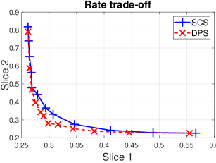
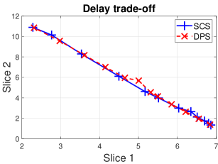
Refer to caption
(a)
Refer to caption
(b)
Figure 3: Delay and throughput trade-offs of single-resource case under asymmetric traffic.
Refer to caption
(a)
Refer to caption
(b)
Figure 4: Delay and throughput trade-offs of single-resource case under symmetric M/D/1 traffic model.

To explain the somewhat surprising result, we conjectured that due to the inter-slice protection built into SCS, under stochastic traffic, the slice with fewer customers tends to see higher processing rate than other sharing criterion, as a result the customers leave the system faster. Overall, SCS tends to separate the busy periods of slices, so that the level of inter-slice contention is reduced. We validated our conjecture by measuring the busy period under the symmetric traffic pattern, where the arrival rates of both slices are the same, and are tuned from 0.05 to 0.45, with s1=s2=0.5subscript𝑠1subscript𝑠20.5s_{1}=s_{2}=0.5. Other parameters are the same as in the setting in Fig. 2. We plot the fraction of times when there is only one busy slice and both slices are busy, vs. the effective traffic intensity ρ=ν1μ1+ν2μ2𝜌subscript𝜈1subscript𝜇1subscript𝜈2subscript𝜇2\rho=\frac{\nu_{1}}{\mu_{1}}+\frac{\nu_{2}}{\mu_{2}} in Fig. 5. One can see that, for both SCS and DPS, the time fraction when both slices are busy increases with ρ𝜌\rho, and that when only one slice is busy first increases when ρ𝜌\rho is low due to underutilization, but decreases when ρ𝜌\rho is high because the inter-slice contention becomes inevitable. However the time fraction when both are busy is always smaller under SCS than that under DPS.
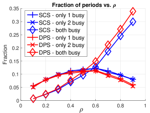
Refer to caption
Figure 5: Busy period of slice 1 and 2 vs. load intensity.

V-B Multiple-resource cases

We also test the performance of SCS under a more complex setting where a simple cellular networks with both fronthaul and backhaul resources are simulated.

Let us consider a setting with 6 fronthaul resources, 3 backhaul resources, and a cloud computing resource. This system supports two slices, each containing 3 user classes. Slice 1 includes Classes 1,2 and 3, while Slice 2 includes Classes 4, 5 and 6. The association between user classes and resources is demonstrated in Fig. 6, and the demand vectors, as well as the arrival rates and mean workloads, are given in Table II.
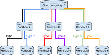
Refer to caption
Figure 6: Association between user classes and resources.

Slice 1’s share is ranged from 0.1 to 0.9, while s2=1s1subscript𝑠21subscript𝑠1s_{2}=1-s_{1}. The achieved performance trade-offs under different sharing criteria are illustrated in Fig. 7. One can see that both SCS and DRF outperform DPS in throughput, with similar mean delays under all 3 criteria. Similar results are observed in a range of settings with different traffic patterns and resource demands. Moreover, in Fig. 8, we adjust the weighting schemes used in DRF by voiding SCWA. Instead, wu=svδu,u𝒰vformulae-sequencesubscript𝑤𝑢subscript𝑠𝑣subscript𝛿𝑢𝑢superscript𝒰𝑣w_{u}=s_{v}\delta_{u},u\in\mathcal{U}^{v}, and the resources are provisioned according to DPS with weight wusubscript𝑤𝑢w_{u}. The results show that without SCWA, DRF is similar to DPS in both throughput and delay. Therefore, we can conclude that SCWA is the root cause of the desirable performance, and SCS can even improve the system performance while providing inter-slice protection.
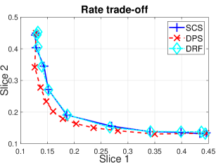
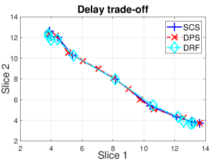
Refer to caption
(a)
Refer to caption
(b)
Figure 7: Performance trade-offs of multi-resource case.
Refer to caption
(a)
Refer to caption
(b)
Figure 8: Performance trade-offs with DRF-weighted DPS.
User Demand vector Mean Arrival
class workload rate
Class 1 (56,0,0,0,0,0,0.5,0,0,0.217)56000000.5000.217(\frac{5}{6},0,0,0,0,0,0.5,0,0,0.217) 1 0.7
Class 2 (0,56,0,0,0,0,0.5,0,0,0.217)05600000.5000.217(0,\frac{5}{6},0,0,0,0,0.5,0,0,0.217) 1 0.7
Class 3 (0,0,1,0,0,0,0,0.625,0,0.217)00100000.62500.217(0,0,1,0,0,0,0,0.625,0,0.217) 1 0.7
Class 4 (0,0,0,1,0,0,0,0.625,0,0.217)00010000.62500.217(0,0,0,1,0,0,0,0.625,0,0.217) 1 0.7
Class 5 (0,0,0,0,1,0,0,0,0.625,0.217)000010000.6250.217(0,0,0,0,1,0,0,0,0.625,0.217) 1 0.7
Class 6 (0,0,0,0,0,1,0,0,0.625,0.217)000001000.6250.217(0,0,0,0,0,1,0,0,0.625,0.217) 1 0.7
TABLE II: Example resource allocation

VI Conclusions and future work

This paper has explored a novel approach to resource allocation for network slicing of distributed resources–SCS, providing inter-slice protection, load-driven elasticity and desirable performance at the same time. SCS can be viewed as a key to enabling low-complexity performance management in network slicing, by exposing network shares to slice operators/tenants, as a high-level resource management interface. This approach can be further extended in two directions: i) if slices have highly imbalanced spatial user distributions, it might be useful to let slices specify different shares across different pools of resources, e.g., regions corresponding to downtown, stadium and/or rural area, see, e.g., [11]; and ii) slices may wish to request different shares across types of resources, e.g., a slice may specify a higher share of computational resource pool than that of the communicational resources. For example, mobile cloud gaming is computation intensive, thus the operator might want to reserve more computing resources than connectivity. Finally, the share abstraction provides a simple parametric “crude” model for slice-level resource allocation which needs to interact with an intra-slice performance management strategy.

References

  • [1] A. Ahmed and E. Ahmed. A survey on mobile edge computing. In 2016 10th International Conference on Intelligent Systems and Control (ISCO), pages 1–8, Jan 2016.
  • [2] E. Altman, K. Avrachenkov, and U. Ayesta. A survey on discriminatory processor sharing. Queueing systems, 53(1-2):53–63, 2006.
  • [3] A. Banchs. User fair queuing: fair allocation of bandwidth for users. In IEEE INFOCOM, volume 3, pages 1668–1677. IEEE, 2002.
  • [4] T. Bonald and L. Massoulié. Impact of fairness on internet performance. In ACM SIGMETRICS Performance Evaluation Review, volume 29, pages 82–91. ACM, 2001.
  • [5] T. Bonald and J. Roberts. Multi-resource fairness: Objectives, algorithms and performance. In ACM SIGMETRICS Performance Evaluation Review, volume 43, pages 31–42. ACM, 2015.
  • [6] F. Bonomi, R. Milito, J. Zhu, and S. Addepalli. Fog computing and its role in the internet of things. In Proceedings of the first edition of the MCC workshop on Mobile cloud computing, pages 13–16. ACM, 2012.
  • [7] S. Boyd and L. Vandenberghe. Convex optimization. Cambridge university press, 2004.
  • [8] S. Brânzei, Y. Chen, X. Deng, A. Filos-Ratsikas, S. K. S. Frederiksen, and J. Zhang. The fisher market game: Equilibrium and welfare. 2014.
  • [9] P. Caballero, A. Banchs, G. de Veciana, and X. Costa-Pêrez. Multi-tenant radio access network slicing: Statistical multiplexing of spatial loads. IEEE/ACM Transactions on Networking, PP(99):1–15, 2017.
  • [10] P. Caballero, A. Banchs, G. de Veciana, and X. Costa-Pérez. Multi-tenant radio access network slicing: Statistical multiplexing of spatial loads. IEEE/ACM Transactions on Networking, 25(5):3044–3058, Oct 2017.
  • [11] P. Caballero, G. de Veciana, A. Banchs, and X. Costa-Perez. Optimizing Network Slicing via Virtual Resource Pool Partitioning (Extended). \urlhttps://www.dropbox.com/s/hso0yqupo5wfwwl/Extended_VRPP.pdf.
  • [12] Y. Cao, H. Song, O. Kaiwartya, B. Zhou, Y. Zhuang, Y. Cao, and X. Zhang. Mobile edge computing for big-data-enabled electric vehicle charging. IEEE Communications Magazine, 56(3):150–156, March 2018.
  • [13] N. Chen and S. Jordan. Throughput in processor-sharing queues. IEEE Transactions on Automatic Control, 52(2):299–305, 2007.
  • [14] J. Dai et al. A fluid limit model criterion for instability of multiclass queueing networks. The Annals of Applied Probability, 6(3):751–757, 1996.
  • [15] J. G. Dai. On positive harris recurrence of multiclass queueing networks: a unified approach via fluid limit models. The Annals of Applied Probability, pages 49–77, 1995.
  • [16] J. G. Dai and S. P. Meyn. Stability and convergence of moments for multiclass queueing networks via fluid limit models. IEEE Transactions on Automatic Control, 40(11):1889–1904, 1995.
  • [17] G. de Veciana, T.-J. Lee, and T. Konstantopoulos. Stability and performance analysis of networks supporting elastic services. IEEE/ACM Transactions on Networking, 9(1):2–14, 2001.
  • [18] J. Dean and S. Ghemawat. Mapreduce: simplified data processing on large clusters. Communications of the ACM, 51(1):107–113, 2008.
  • [19] M. Feldman et al. The proportional-share allocation market for computational resources. IEEE TPDS, 20(8):1075–1088, 2009.
  • [20] A. Ghodsi, M. Zaharia, B. Hindman, A. Konwinski, S. Shenker, and I. Stoica. Dominant resource fairness: Fair allocation of multiple resource types. In Nsdi, volume 11, pages 24–24, 2011.
  • [21] T. Guo and R. Arnott. Active lte ran sharing with partial resource reservation. In Vehicular Technology Conference (VTC Fall), 2013 IEEE 78th, pages 1–5. IEEE, 2013.
  • [22] T. Lan, D. Kao, M. Chiang, and A. Sabharwal. An axiomatic theory of fairness in network resource allocation. In 2010 Proceedings IEEE INFOCOM, pages 1–9, March 2010.
  • [23] J. Mo and J. Walrand. Fair end-to-end window-based congestion control. IEEE/ACM Transactions on Networking, 8(5):556–567, Oct 2000.
  • [24] H. Moulin. Fair division and collective welfare. MIT press, 2004.
  • [25] N. Nisan, T. Roughgarden, E. Tardos, and V. V. Vazirani. Algorithmic game theory, volume 1. Cambridge University Press Cambridge, 2007.
  • [26] M. Pióro and D. Medhi. Routing, flow, and capacity design in communication and computer networks. Elsevier, 2004.
  • [27] M. Satyanarayanan. The emergence of edge computing. Computer, 50(1):30–39, 2017.
  • [28] O. Soliman, A. Rezgui, H. Soliman, and N. Manea. Mobile cloud gaming: Issues and challenges. In International Conference on Mobile Web and Information Systems, pages 121–128. Springer, 2013.
  • [29] R. Srikant and L. Ying. Communication networks: an optimization, control, and stochastic networks perspective. Cambridge University Press, 2013.
  • [30] M. J. van Uitert. Generalized processor sharing queues. Eindhoven University of Technology, 2003.
  • [31] H. R. Varian. Equity, envy, and efficiency. 1973.
  • [32] Wikipedia contributors. Norm (mathematics) — Wikipedia, the free encyclopedia, 2018. [Online; accessed 21-December-2018].
  • [33] H. P. Young. Equity: in theory and practice. Princeton University Press, 1995.
  • [34] J. Zheng, P. Caballero, G. de Veciana, S. J. Baek, and A. Banchs. Statistical multiplexing and traffic shaping games for network slicing. IEEE/ACM Transactions on Networking, 26(6):2528–2541, Dec 2018.