A Conway-Maxwell-Poisson GARMA Model for Count Data

Abstract

We propose a flexible model for count time series which has potential uses for both underdispersed and overdispersed data. The model is based on the Conway-Maxwell-Poisson (COM-Poisson) distribution with parameters varying along time to take serial correlation into account. Model estimation is challenging however and require the application of recently proposed methods to deal with the intractable normalising constant as well as efficiently sampling values from the COM-Poisson distribution.

Key words: Bayesian methods, COM-Poisson, Generalized ARMA, Intractable likelihood.

1 Introduction

Time series of counts are abundant in many areas of science and their statistical analysis has received considerable attention. For example, Zeger (1988) and Chan and Ledolter (1995) studied Poisson generalized linear models where the mean follows a latent autoregressive process. Models for count time series embedded in the framework of integer valued ARMA type models have also been discussed in the literature (see for example Davis et al. (1999) for an overview and also Biswas and Song (2009)). Generalized autoregressive moving average (GARMA) models, introduced by Benjamin et al. (2003) and extended in Andrade et al. (2015) for a Bayesian approach, have potential uses for modeling overdispersed time series count data. In this paper, we consider a more flexible model making use of the Conway-Maxwell-Poisson (COM-Poisson) distribution which allows the mean and the variance of count data to be modelled separetely and also handles underdispersion (besides overdispersion).

Suppose the discrete random variable $Y$ represents count data with can present underdispersion, overdispersion, or equidispersion. A flexible distribution to model such data is the Conway-Maxwell-Poisson (COM-Poisson, Conway and Maxwell (1962)) distribution for which the probability mass function is given by,

$$p(y|\mu,\nu)=\left(\frac{\mu^{y}}{y!}\right)^{\nu}\frac{1}{Z(\mu,\nu)},~{}\mu>0,\nu>0,~{}y=0,1,2,\dots,$$

where $Z(\mu,\nu)=\sum_{y=0}^{\infty}\left(\mu^{\nu}/y!\right)^{\nu}$ is an intractable normalising constant, having no closed form representation for $\nu\neq 1$. This is the reparameterization proposed by Guikema and Goffelt (2018). Clearly the Poisson distribution with parameter $\mu$ is a particular case when $\nu=1$, in which case it exhibits equidispersion. Otherwise, the distribution will exhibit underdispersion ($\nu>1$) or overdispersion ($\nu<1$).

The mode of the distribution is given by $\lfloor{\mu}\rfloor$, i.e. the largest integer below $\mu$ and there are two modes $\mu$ and $\mu-1$ if $\mu$ is integer. Clearly, the moments of the distribution are not available in closed form as a consequence of the intractable normalising constant $Z(\mu,\nu)$. Approximations for the mean and the variance are given by,

$$E(Y)\approx\mu+\frac{1}{2\nu}-\frac{1}{2}\quad\mbox{and}\quad Var(Y)\approx\frac{\mu}{\nu}$$ (1)

which are based on an asymptotic representation of $Z(\mu,\nu)$ (Minka et al. (2003), Shmueli et al. (2005)). If $\mu$ or $\nu$ (or both) are not small then these approximations are quite accurate in which case $\mu$ closely approximates $E(Y)$.

Moments of the COM-Poisson can also be written in terms of derivatives of the normalising constant and, as shown in Minka et al. (2003), approximate expressions are obtained from its asymptotic approximation,

$$E(Y) = \frac{\mu}{\nu}~{}\frac{\partial\log Z(\mu,v)}{\partial\mu}$$

$$E[\log Y!] = -\frac{\partial\log Z(\mu,v)}{\partial\nu}\approx\frac{1}{2\nu}\log\mu+\mu(\log\mu-1).$$ (2)

The main contributions in this paper are, to propose a COM-Poisson model with a Generalized ARMA (GARMA) structure for the mean of time series of counts as well as a Bayesian approach to estimate parameters and compare models. This will in turn require the application of recently proposed methods to deal with the intractable normalising constant as well as efficiently sampling values from the COM-Poisson distribution.

The remainder of this paper is organized as follows. In Section 2, the model adopted for a time series of counts and the methods used to estimate parameter and make predictions are described. Examples of applications are provided in Section 3 where an overdispersed time series of counts is analysed. Section 4 concludes the paper.

2 Model Description and Methods

For a time series $y_{1},\dots,y_{n}$ we assume that the conditional probability mass function of each $y_{t}$ given the previous information set $\mathcal{F}_{t-1}=\{y_{1},\dots,y_{t-1},\mu_{1},\dots,\mu_{t-1},\nu_{1},\dots,\nu_{t-1}\}$ is given by,

$$p(y_{t}|\mathcal{F}_{t-1})=\left(\frac{\mu_{t}^{y_{t}}}{y_{t}!}\right)^{\nu_{t}}\frac{1}{Z(\mu_{t},\nu_{t})}=\frac{q(y_{t}|\mathcal{F}_{t-1})}{Z(\mu_{t},\nu_{t})},$$ (3)

where $q(y_{t}|\mathcal{F}_{t-1})$ is the unnormalised conditional probability of each $y_{t}$ assuming values $0,1,2,\dots$ and $Z(\mu_{t},\nu_{t})$ is the associated normalising constant. Since the COM-Poisson distribution is a member of the exponential family we propose to extend the idea in GARMA models introduced by Benjamin et al. (2003), and assume the following linear predictor for the COM-Poisson model,

$$\log(\mu_{t})=\sum_{j=1}^{p}\phi_{j}\log(y_{t-j})+\sum_{j=1}^{q}\theta_{j}\{\log(y_{t-j}/\mu_{t-j})\},$$

thus accounting for the autocorrelation structure present in the data. In practice, this expression is evaluated using $y_{t-j}^{*}=\max(y_{t-j},c)$ with $0<c<1$ since each $y_{t}$ can assume a value zero. In particular, if $\nu=1$ in (3) this model reduces to the Poisson-GARMA model as studied for example in Andrade et al. (2015). We also consider a relationship between the dispersion parameter $\nu_{t}$ and lagged values of the time series using a logarithm link function,

$$\log(\nu_{t})=\sum_{j=1}^{p}\delta_{j}\log(y_{t-j})$$

Now let $\hbox{\boldmath$\theta$}\in\mathbb{R}^{d}$ denote a $d$-dimensional vector of parameters in the GARMA specification. Then, the partial likelihood function for a COM-Poisson GARMA($p,q$) model is given by,

$$p(\hbox{\boldmath$y$}|\hbox{\boldmath$\theta$})=\prod_{t=r+1}^{n}p(y_{t}|\mathcal{F}_{t-1})=\prod_{t=r+1}^{n}\left(\frac{\mu_{t}^{y_{t}}}{y_{t}!}\right)^{\nu_{t}}\frac{1}{Z(\mu_{t},\nu_{t})},$$

which clearly involves multiple intractable normalising constants. The log-likelihood is given by,

$$\log p(\hbox{\boldmath$y$}|\hbox{\boldmath$\theta$}) = \sum_{t=r+1}^{n}\log p(y_{t}|\mathcal{F}_{t-1})$$

$$= \sum_{t=r+1}^{n}\nu_{t}y_{t}\log\mu_{t}-\sum_{t=r+1}^{n}\nu_{t}\log y_{t}!-\sum_{t=r+1}^{n}\log Z(\mu_{t},\nu_{t}).$$

In the Bayesian approach we also place a prior distribution on $\theta$ with density $p(\hbox{\boldmath$\theta$})$ and the, by Bayes theorem, the posterior distribution is given by,

$$p(\hbox{\boldmath$\theta$}|\hbox{\boldmath$y$})\propto\prod_{t=r+1}^{n}p(y_{t}|\mathcal{F}_{t-1})~{}p(\hbox{\boldmath$\theta$}),$$

which is now a doubly-intractable posterior distribution since it depends on integrating the right hand side which is itself intractable. In terms of simulation, a direct application of the Metropolis-Hastings algorithm would propose a candidate value $\hbox{\boldmath$\theta$}^{\prime}\sim h(\cdot|\hbox{\boldmath$\theta$})$ and accept this move with probability,

$$\alpha(\hbox{\boldmath$\theta$},\hbox{\boldmath$\theta$}^{\prime})=\min\left\{1,\frac{\prod_{t=r+1}^{n}q(y_{t}|\mathcal{F}_{t-1}^{\prime})~{}p(\hbox{\boldmath$\theta$}^{\prime})~{}h(\hbox{\boldmath$\theta$}|\hbox{\boldmath$\theta$}^{\prime})}{\prod_{t=r+1}^{n}q(y_{t}|\mathcal{F}_{t-1})~{}p(\hbox{\boldmath$\theta$})~{}h(\hbox{\boldmath$\theta$}^{\prime}|\hbox{\boldmath$\theta$})}~{}\frac{\prod_{t=r+1}^{n}Z(\mu_{t},\nu_{t})}{\prod_{t=r+1}^{n}Z(\mu_{t}^{\prime},\nu_{t}^{\prime})}\right\}.$$

where,

$$\log(\mu_{t}^{\prime})=\sum_{j=1}^{p}\phi_{j}^{\prime}\log(y_{t-j})+\sum_{j=1}^{q}\theta_{j}^{\prime}\{\log(y_{t-j})-\log(\mu_{t-j}^{\prime})\},$$

and $\mathcal{F}_{t-1}^{\prime}=\{y_{1},\dots,y_{t-1},\mu_{1}^{\prime},\dots,\mu_{t-1}^{\prime}\}$.

It is therefore not computionally feasable to update the parameters $\theta$ using the standard Metropolis-Hastings algorithm. One way round this problem is to use the so called exchange algorithm proposed by Murray et al. (2006) which extends the algorithm in Møller et al. (2006) and basically augments the posterior state space with auxiliary data drawn from the likelihood. The idea is to include one further step by proposing values $\hbox{\boldmath$y$}^{\prime}=(y_{1}^{\prime},\dots,y_{n}^{\prime})$ given $\hbox{\boldmath$\theta$}^{\prime}$ and define the joint distribution,

$$p(\hbox{\boldmath$y$},\hbox{\boldmath$y$}^{\prime},\hbox{\boldmath$\theta$},\hbox{\boldmath$\theta$}^{\prime})\propto\prod_{t=r+1}^{n}\frac{q(y_{t}|\mathcal{F}_{t-1})}{Z(\mu_{t},\nu_{t})}p(\hbox{\boldmath$\theta$})h(\hbox{\boldmath$\theta$}^{\prime}|\hbox{\boldmath$\theta$})\prod_{t=r+1}^{n}\frac{q(y_{t}^{\prime}|\mathcal{F}_{t-1}^{*})}{Z(\mu_{t}^{\prime},\nu_{t}^{\prime})}.$$

Note that the information set was redefine as $\mathcal{F}_{t-1}^{*}=\{y_{1}^{\prime},\dots,y_{t-1}^{\prime},\mu_{1}^{\prime},\dots,\mu_{t-1}^{\prime}\}$ since each $y_{t}^{\prime}$ is generate sequentially from the distribution of $y_{t}|\mathcal{F}_{t-1}^{*}$. The acceptance probability now becomes,

$$\alpha(\hbox{\boldmath$\theta$},\hbox{\boldmath$\theta$}^{\prime})=\min\left\{1,\frac{\prod_{t=r+1}^{n}q(y_{t}|\mathcal{F}_{t-1}^{\prime})~{}p(\hbox{\boldmath$\theta$}^{\prime})~{}h(\hbox{\boldmath$\theta$}|\hbox{\boldmath$\theta$}^{\prime})}{\prod_{t=r+1}^{n}q(y_{t}|\mathcal{F}_{t-1})~{}p(\hbox{\boldmath$\theta$})~{}h(\hbox{\boldmath$\theta$}^{\prime}|\hbox{\boldmath$\theta$})}\frac{\prod_{t=r+1}^{n}q(y_{t}^{\prime}|\mathcal{F}_{t-1})}{\prod_{t=r+1}^{n}q(y_{t}^{\prime}|\mathcal{F}_{t-1}^{*})}\right\}.$$

thus avoiding the need to evaluate a set of intractable normalising constants which cancelled out. Note that the ratio of normalising constants $Z(\mu_{t},\nu)/Z(\mu_{t}^{\prime},\nu_{t}^{\prime})$ is actually being replaced by the ratio of unnormalised probabilities $q(y_{t}^{\prime}|\mathcal{F}_{t-1})/q(y_{t}^{\prime}|\mathcal{F}_{t-1}^{\prime})$.

Since the exchange algorithm relies on sampling each auxiliary variable $y_{t}^{\prime}|\mathcal{F}_{t-1}^{*}$, $t=r+1,\dots,n$ from the COM-Poisson likelihood we need this sampler to be computationally efficient. Also, it requires exact draws from the likelihood given each parameter value and this is the case for the sampler adopted in this paper and described in the next section.

2.1 Sampling from the COM-Poisson Distribution

Rewrite the probability mass function as,

$$p(y|\mu,\nu)=q(y|\mu,\nu)/Z(\mu,\nu)$$

where $Z(\mu,\nu)=\sum_{y=0}^{\infty}q(y|\mu,\nu)$ and consider an envelope density function given by,

$$g(y)=q_{g}(y)/Z_{g},$$

where $Z_{g}=\sum_{y=0}^{\infty}q_{g}(y)$. For a finite bounding constant $M$ the envelope inequality is given by $Mg(y)>p(y|\mu,\nu)$. Then, a rejection sampling scheme would be to draw a value $y^{*}$ from $g(\cdot)$ and accept $y^{*}$ as a draw from $p(\cdot|\mu,\nu)$ with probability,

$$\alpha(y^{*})=\frac{p(y^{*}|\mu,\nu)}{Mg(y^{*})}.$$

This is however clearly intractable if either $Z(\mu,\nu)$ or $Z_{g}$ is intractable. Likewise, the optimal value of the constant $M$ which is given by $\sup_{y}\{p(y|\mu,\nu)/g(y)\}$ is also impossible to obtain for intractable likelihoods.

Recently, Chanialidis et al. (2018) and Benson and Friel (2017) proposed rejection sampling schemes to draw values from the COM-Poisson distribution without the need to evaluate the normalising constant. Chanialidis et al. (2018) proposed a rejection sampling scheme using an auxiliary piecewise geometric distribution for which the normalising constant is given in closed form. Benson and Friel (2017) proposed a considerably simpler approach which is more useful in the context of time series models where we need to draw each $y_{t}|\mathcal{F}_{t-1}$, $t=1,2\dots$. The scheme is briefly described below.

Upper Bound Approach

In the rejection sampler, we note that the optimal value of the bounding constant can be rewritten as,

$$M = \sup_{y}\left\{\frac{p(y|\mu,\nu)}{g(y)}\right\}=\frac{1/Z(\mu,\nu)}{1/Z_{g}}\sup_{y}\left\{\frac{q(y|\mu,\nu)}{q_{g}(y)}\right\}=\frac{Z_{g}}{Z(\mu,\nu)}B,$$

where the constant $B=\sup_{y}\{q(y|\mu,\nu)/q_{g}(y)\}$ is tractable. The acceptance probability is then given by,

$$\alpha(y^{*})=\frac{p(y^{*}|\mu,\nu)}{\frac{Z_{g}}{Z(\mu,\nu)}B~{}g(y^{*})}=\frac{q(y^{*}|\mu,\nu)}{B~{}q_{g}(y^{*})}.$$

Benson and Friel (2017) then showed that we can sample from the COM-Poisson with parameters $\mu$ and $\nu$ by using a Poisson($\mu$) envelope with bounding constant,

$$B=\left(\frac{\mu^{\lfloor\mu\rfloor}}{\lfloor\mu\rfloor!}\right)^{\nu-1}=q(\lfloor\mu\rfloor,\mu,\nu-1),$$

if $\nu\geq 1$ and a Geometric($p$) envelope with bounding constant,

$$B=\left(\frac{\mu^{\lambda}}{\lambda!}\right)^{\nu}\frac{1}{(1-p)^{\lambda}p}=q(\lambda,\mu,\nu)\frac{1}{(1-p)^{\lambda}p},$$

if $\nu<1$ with $\lambda=\lfloor\mu/(1-p)^{1/\nu}\rfloor$. The value of $p$ in the geometric distribution should be chosen so as to maximise the acceptance rate of the sampler but this optimal value is infeasible to compute as it involves intractable normalising constants. Benson and Friel (2017) proposed to chose $p$ by matching the geometric mean $(1-p)/p$ to the approximate COM-Poisson mean $\mu+1/2\nu-1/2$ which results in $p=2\nu/(2\mu\nu+1+\nu)$. This is also the approach adopted here as it proved very efficient in our applications.

Finally, for the bounding constants above the acceptance probabilities for a proposed value $y^{*}$ are given by,

$$\alpha(y^{*})=\frac{q(y^{*},\mu,\nu)}{q(\lfloor\mu\rfloor,\mu,\nu-1)q(y^{*},\mu,1)}$$

if $\nu\geq 1$ and,

$$\alpha(y^{*})=\frac{q(y^{*},\mu,\nu)(1-p)^{\lambda}p}{q(\lambda,\mu,\nu)(1-p)^{y^{*}}p},$$

if $\nu<1$.

2.2 Prior distributions

The GARMA coefficients in the COM-Poisson GARMA model are defined in the real line. Therefore, we assign independent normal prior distributions centered about zero to these coefficients. The prior variances $\sigma_{\phi}^{2}$, $\sigma_{\theta}^{2}$ and $\sigma_{\delta}^{2}$ are chosen so as to reflect vague prior knowledge on these coefficients.

2.3 Bayesian Predictions

An important aspect of a time series model is its ability to predict future values of the series. Given the observed time series $\hbox{\boldmath$y$}=\{y_{1},\dots,y_{n}\}$, the one-step ahead predictive probability mass function is given by,

$$p(y_{n+1}|\hbox{\boldmath$y$})=\int p(y_{n+1}|\hbox{\boldmath$y$},\hbox{\boldmath$\theta$})p(\hbox{\boldmath$\theta$}|\hbox{\boldmath$y$})d\hbox{\boldmath$\theta$},$$

which is not available in closed form. However, given a sample of size $N$, $\hbox{\boldmath$\theta$}^{1},\dots,\hbox{\boldmath$\theta$}^{N}$ from the posterior distribution of $\theta$ a Monte Carlo approximation is given by,

$$\hat{p}(y_{n+1}|\hbox{\boldmath$y$})=\frac{1}{N}\sum_{j=1}^{N}p(y_{n+1}|\hbox{\boldmath$y$},\hbox{\boldmath$\theta$}^{j}).$$ (4)

An approximation for the conditional probability mass function $p(y_{n+1}|\hbox{\boldmath$y$},\hbox{\boldmath$\theta$})$ in turn is obtained by generating $y_{n+1}^{j,1},\dots,y_{n+1}^{j,L}$ from a COM-Poisson distribution with parameters $\mu_{n+1}^{j}$ and $\nu_{n+1}^{j}$ which are computed conditional on $\hbox{\boldmath$\theta$}^{j}$. This allows us to approximate the conditional probabilities in (4) by the sample proportions of $y_{n+1}^{j}=k$, $k=0,1,\dots$ and then calculate $\hat{p}(y_{n+1}|\hbox{\boldmath$y$})$ accordingly.

3 Application

The first real data set analysed is the time series with the monthly number of cases of poliomyelitis in the United States between 1970 and 1983 (Zeger (1988)). The data (198 observations) are depicted as a time series in Figure 1. The mean and variance of this series are $1.33$ and $3.5$ respectively which together with the histogram in Figure 1 clearly indicate overdispersion. The following model was estimated,

$$Y_{t}|\mathcal{F}_{t-1} \sim \mbox{COM-Poisson}(\mu_{t},\nu_{t}),$$

$$\log(\mu_{t}) = \phi\log(y_{t-1}+\theta\log(y_{t-1}/\mu_{t-1})$$

$$\log(\nu_{t}) = \delta\log(y_{t-1}.$$

for $t=1,\dots,n$.

The results shown in this section are based on running the proposed sampler for 100,000 iterations, discarding the first 50,000 as burn-in and skipping every 10th. This resulted in a final sample of 5000 values from the posterior distribution. The parameters were updated jointly and a simple random walk Metropolis was employed to propose new values using normal proposal distributions centered about the current values with proposal variances tuned to achieve an acceptance rate about 0.48.

Figure 2 shows traces and the sample autocorrelations for the coefficients from which we notice both good mixing in the parameter space and autocorrelations vanishing fairly rapidly. Figure 3 shows the observed counts (as vertical lines) together with estimates of $\mu_{t}$ given the sampled values of coefficients while Figure 4 shows the estimated one-step ahead predicitive distribution using the approach described in Section 2.3.

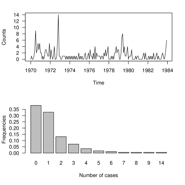
Figure 1: The monthly number of cases of poliomyelitis in the United States between 1970 and 1983 and the associated frequencies.

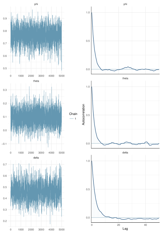
Figure 2: Trace and autocorrelation plots of the MCMC draws.

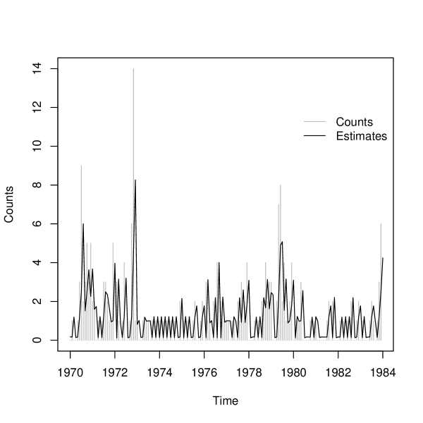
Figure 3: Monthly number of cases of poliomyelitis in the United States between 1970 and 1983 and estimated $\mu_{t}$.

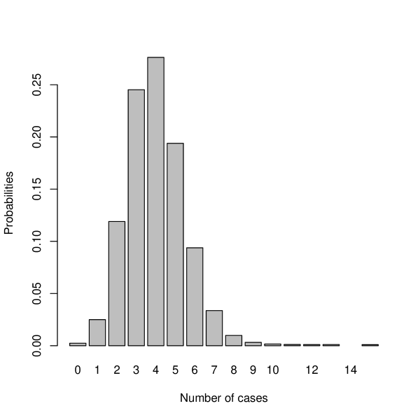
Figure 4: Predictive one-step ahead distribution of the number of cases of poliomyelitis in the United States.

4 Conclusions

As pointed out in Sellers et al. (2012), when dealing with count data where the Poisson distribution plays an important role we should try and extend the analysis to incorporate both overdispersion and underdispersion features in the model. This is much so for time series of counts where the degree of dispersion can additionally vary along time.

Based on advantages of using the COM-Poisson distribution to model overdispersed and underdispersed data and recent advances on computations for doubly intractable problems we proposed a COM-Poisson GARMA model for time series of counts. Model parameters were estimated using simulation based MCMC methods and the exchange algorithm coupled with a recently proposed clever way of generating values from a COM-Poisson distribution. This COM-Poisson generator was also useful to obtain the out-of-sample one-step ahead predictive distribution.

This is an ongoing work and the author is investingating ways to perform model comparison which is challenging in the context of intractable likelihoods.

References

- Andrade et al. (2015) B.S. Andrade, M.G. Andrade, and R.S. Ehlers. Bayesian GARMA models for count data. Communications in Statistics: Case Studies, Data Analysis and Applications, 1(4):192–205, 2015.
- Benjamin et al. (2003) M. A. Benjamin, R. A. Rigby, and D. M. Stasinopoulos. Generalized autoregressive moving average models. Journal of the American Statistical Association, 98:214–223, 2003.
- Benson and Friel (2017) A. Benson and N. Friel. Bayesian inference, model selection and likelihood estimation using fast rejection sampling: the Conway-Maxwell-Poisson distribution. ArXiv e-prints, 2017.
- Biswas and Song (2009) Atanu Biswas and Peter X.-K. Song. Discrete-valued ARMA processes. Statistics and Probability Letters, 79(17):1884–1889, 2009.
- Chan and Ledolter (1995) K. Chan and J. Ledolter. Monte Carlo EM estimation for time series models involving counts. Journal of the American Statistical Association, 90:242–251, 1995.
- Chanialidis et al. (2018) Charalampos Chanialidis, Ludger Evers, Tereza Neocleous, and Agostino Nobile. Efficient Bayesian inference for COM-Poisson regression models. Statistics and Computing, 28(3):595–608, 2018.
- Conway and Maxwell (1962) R. W. Conway and W. L. Maxwell. A queuing model with state dependent service rates. Journal of Industrial Engineering, 12(2):132–136, 1962.
- Davis et al. (1999) R. A. Davis, W. T. Dunsmuir, and Y. Wang. Modelling time series of counts data. Asymptotic, Nonparametric, and Time Series, Ed. S. Ghosh:63–114, 1999.
- Guikema and Goffelt (2018) Seth D. Guikema and Jeremy P. Goffelt. A flexible count data regression model for risk analysis. Risk Analysis, 28(1):213–223, 2018.
- Lyne et al. (2015) Anne-Marie Lyne, Mark Girolami, Yves Atchadé, Heiko Strathmann, and Daniel Simpson. On russian roulette estimates for Bayesian inference with doubly-intractable likelihoods. Statistical Science, 30(4):443–467, 2015.
- Minka et al. (2003) T.P. Minka, G. Shmueli, J.B. Kadane, S. Borle, and P. Boatwright. Computing with the COM-Poisson distribution. Technical Report 776, Department of Statistics, Carnegie Mellon University, 2003.
- Møller et al. (2006) J. Møller, A.N. Pettitt, R. Reeves, and K.K. Berthelsen. An efficient Markov chain Monte Carlo method for distributions with intractable normalising constants. Biometrika, 93(2):451–458, 2006.
- Murray et al. (2006) I. Murray, Z. Ghahramani, and D. MacKay. MCMC for doubly-intractable distributions. In R. Dechter and T. Richardson, editors, Uncertainty in Artificial Intelligence, pages 359–366. AUAI Press, 2006.
- Sellers et al. (2012) K. F. Sellers, S. Borle, and G. Shmueli. The COM-Poisson model for count data: a survey of methods and applications. Applied Stochastic Models in Business and Industry, 28(2):104–116, 2012.
- Shmueli et al. (2005) Galit Shmueli, Tom Minka, Joseph B. Kadane, Sharad Borle, and Peter Boatwright. A useful distribution for fitting discrete data: Revival of the Conway-Maxwell-Poisson distribution. Journal of the Royal Statistical Society: Series C (Applied Statistics), 54(1):127–142, 2005.
- Zeger (1988) S. L. Zeger. A regression model for time series of counts. Biometrika, 75(4):621–629, 1988.