A posteriori error estimates for the monodomain model in cardiac electrophysiology

Abstract

We consider the monodomain model, a system of a parabolic semilinear reaction-diffusion equation coupled with a nonlinear ordinary differential equation, arising from the (simplified) mathematical description of the electrical activity of the heart. We derive a posteriori error estimators accounting for different sources of error (space/time discretization and linearization). We prove reliability and efficiency (this latter under a suitable assumption) of the error indicators. Finally, numerical experiments assess the validity of the theoretical results.

1 Introduction

The main goal of this paper is the a posteriori numerical analysis of the monodomain model, a system of a parabolic semilinear reaction-diffusion equation coupled with a nonlinear ordinary differential equation, arising from the mathematical description of the electrical activity of the heart. The monodomain model represents a simplified version of the more realistic bidomain model which has been object in recent years of an intense research activity, see e.g. [9] and references therein. For the purpose of the paper, we first recall [12], where a careful a priori analysis of the Galerkin semidiscrete space approximation of the bidomain system is performed, investigating convergence properties and stability estimates for the semidiscrete solution. This result, coupled with the argument regarding the time-discretization analysis provided in [10], allows for an exhaustive a priori error analysis for the bidomain model. Moreover, in [8] the authors introduce a space-time adaptive algorithm for the solution of the bidomain model by resorting to a stepsize control for the temporal adaptivity, whereas spatial adaptivity is performed by virtue of a posteriori local error estimators. However, a complete a posteriori error analysis is missing.

With the aim of contributing to fill this gap, in this paper we focus on the simpler monodomain model and provide a detailed a posteriori analysis. In particular, we consider a Newton-Galerkin approximation of the monodomain system and look for a posteriori indicators of the error involving the $L^{2}(0,T;H^{1}(\Omega))$ norm. Inspired by the seminal work [17] and by the recent papers [11, 1], we derive a posteriori error bounds by providing a suitable splitting of the total residual into three operators, accounting for different sources of error entailed by the discretization process. Specifically, we introduce a linearization residual, a time discretization residual, and a space discretization residual, with the additional difficulty with respect, e.g., to [1] represented by the coupled structure of the system of differential equations.

The a posteriori analysis is complemented with an a priori analysis which relies on previous results obtained in [13], where error estimates with respect to the $L^{\infty}(0,T;L^{2}(\Omega))$ norm of the error are obtained. Here, we derive a priori estimates for the semidiscrete problem in a different norm involving the $L^{2}(0,T;H^{1}(\Omega))$ one.

The a posteriori error estimators obtained in this paper can be employed to derive fully space-time adaptive algorithms that can be of particular importance, for instance, in the solution of inverse problems like the identification of ischemic regions (i.e. areas in which the coefficient of the system are altered from the reference values) by means of boundary voltage. An iterative algorithm (as the one proposed in [3] for a simplified model) would greatly benefit from an adaptive approach that would drastically reduce the computational cost.

The paper is organized as follows: in Section 2 we introduce the Newton-Galerkin full discretization of the monodomain model, whereas Section 3 is devoted to the a priori estimates for the problem. In Section 4 we introduce the residual operators associated to the discrete solution and prove the equivalence between the error and the residual (in suitable norms). In Section 5 we define three a posteriori estimators and employ them to prove an upper bound for the approximation error. We also provide, under a suitable assumption, a lower estimate for the error in terms of the same indicators, thus assessing their efficiency. Finally, Section 6 reports some numerical experiments assessing the validity of the derived estimates and investigating convergence rates both of the error and of the estimators as the discretization parameters are reduced.

2 A Newton-Galerkin scheme for the approximation of the monodomain model

Let $\Omega\subset\mathbb{R}^{d}$, $d=2,3$, be an open bounded domain. Consider the monodomain model (see [9, 14])

$$\left\{\begin{aligned} \partial_{t}u-\nabla\cdot(M\nabla u)+f(u,w)&=0\qquad&\text{in }\Omega\times(0,T),\\ M\partial_{\nu}u&=0\qquad&\text{on }\partial\Omega\times(0,T),\\ u|_{t=0}&=u_{0}\qquad&\text{in }\Omega,\\ \partial_{t}w+g(u,w)&=0\qquad&\text{in }\Omega\times(0,T),\\ w|_{t=0}&=w_{0}\qquad&\text{in }\Omega,\end{aligned}\right.$$ (2.1)

being $u$ the trasmembrane electrical potential in the cardiac tissue and $M:\Omega\rightarrow\mathbb{R}^{d\times d}$ the conductivity tensor. In particular, according to the biological application, we assume that $M$ is constant in time, and in each point $x\in\Omega$ the tensor $M(x)$ is a symmetric positive definite matrix, with positive eigenvalues $\mu_{i}$, $i=1,\ldots,d$. Moreover, we suppose that $\mu_{i}(x)$ are uniform in space and denote by $\mu_{min}$ and $\mu_{max}$ the minimum and the maximum eigenvalue, respectively. The associated eigenvectors may instead vary in space, and we assume that the overall matrix function $M(x)$ is smooth. The nonlinear term $f(u,w)$ models the current induced by the motion of ions across the membrane, and is addressed as ionic current. According to a well established phenomenological approach (see, e.g., [14]), $f$ is a function of the potential $u$ and of a recovery variable $w$, whose dynamics is governed by a coupled nonlinear ordinary differential equation involving a nonlinear term $g$. We focus in particular on the Aliev-Panfilov model of the cardiac tissue, according to the version reported, e.g., in [4]; namely, the nonlinear terms $f$ and $g$ are as follows:

$$f(u,w)=Au(u-a)(u-1)+uw,\qquad g(u,w)=\epsilon(Au(u-1-a)+w),$$ (2.2)

with $A,\epsilon>0$, $0<a<1$. Such a problem is showed to be well-posed: in particular, we refer to [2], which extends the results contained in [13] to the model of interest, and guarantees the following existence, uniqueness and comparison result:

Proposition 2.1.

Let the initial data $u_{0}\in C^{2+\alpha}(\bar{\Omega})$, $w_{0}\in C^{\alpha}(\bar{\Omega})$ satisfy the bound $0\leq u_{0}\leq 1$ and $0\leq w_{0}\leq\frac{A(1+a)^{2}}{4}$, consider $M\in C^{2}(\Omega)$ and let the following compatibility conditions hold: $M\nabla u_{0}\cdot\nu=0$, being $\partial\Omega\in C^{2+\alpha}$. Then, there exists a unique classical solution $(u,w)$ of (2.1), $u\in C^{2+\alpha,1+\alpha/2}(\overline{\Omega}\times[0,T])$ and $w\in C^{\alpha,1+\alpha/2}(\overline{\Omega}\times[0,T])$. Moreover, it holds that

$$0\leq u(x,t)\leq 1,\quad 0\leq w(x,t)\leq\frac{A(1+a)^{2}}{4}\qquad\forall(x,t)\in\Omega\times(0,T).$$

Remark 2.1.

When considering $w_{0}\in C^{2+\alpha}(\bar{\Omega})$, one can easily conclude (see [2]) that also $w\in C^{2+\alpha,1+\alpha/2}(\overline{\Omega}\times[0,T])$. In particular, both $u(\cdot,t)$ and $w(\cdot,t)$ belong to the Sobolev’s space $H^{2}(\Omega)$ for each $t\in[0,T]$.

Remark 2.2.

If the conductivity tensor $M$ is only in $L^{\infty}(\Omega)$ (as in the case of an ischemic heart), we can nevertheless show ([2]) the existence and uniqueness of the weak solution $(u,w)$ s.t. $u\in L^{2}(0,T;H^{1}(\Omega))\cap L^{\infty}(0,T;L^{2}(\Omega))$, $\partial_{t}u\in L^{2}(0,T;H^{*})$, $w\in L^{\infty}(0,T;L^{2}(\Omega))$, $\partial_{t}w\in L^{2}((0,T)\times\Omega)$, where $H^{*}=(H^{1}(\Omega))^{*}$. Moreover, the same bounds on $u,w$ hold as above and it is possible to guarantee additional regularity on the solution, namely $u\in C^{\alpha,\alpha/2}(\overline{\Omega}\times[0,T])$, $w\in C^{\alpha,1+\alpha/2}(\overline{\Omega}\times[0,T])$.

The weak formulation of (2.1) reads

$$\left\{\begin{aligned} \int_{\Omega}\partial_{t}u\varphi dx+\int_{\Omega}M\nabla u\cdot\nabla\varphi dx+\int_{\Omega}f(u,w)\varphi dx&=0\qquad\forall\varphi\in H^{1}(\Omega),\\ \int_{\Omega}\partial_{t}w\psi dx+\int_{\Omega}g(u,w)\psi dx&=0\qquad\forall\psi\in L^{2}(\Omega).\end{aligned}\right.$$ (2.3)

For each time interval $(t_{a},t_{b})\subset(0,T)$, we introduce the following functional spaces:

$$X(t_{a},t_{b}) =\{u\textit{ s.t. }u\in L^{2}(t_{a},t_{b};H^{1}(\Omega))\cap L^{\infty}(t_{a},t_{b};L^{2}(\Omega)),\partial_{t}u\in L^{2}(t_{a},t_{b};H^{*})\}$$

$$Y(t_{a},t_{b}) =\{w\textit{ s.t. }w\in L^{\infty}(t_{a},t_{b};L^{2}(\Omega)),\partial_{t}w\in L^{2}((t_{a},t_{b})\times\Omega)\},$$

which are Banach spaces endowed with the norms:

$${\left\|u\right\|}_{X(t_{a},t_{b})} =\left({\left\|u\right\|}_{L^{2}(t_{a},t_{b};H^{1}(\Omega))}^{2}+{\left\|u\right\|}_{L^{\infty}(t_{a},t_{b};L^{2}(\Omega))}^{2}+{\left\|\partial_{t}u\right\|}_{L^{2}(t_{a},t_{b};H^{*})}^{2}\right)^{\frac{1}{2}}$$

$${\left\|w\right\|}_{Y(t_{a},t_{b})} =\left({\left\|w\right\|}_{L^{\infty}(t_{a},t_{b};L^{2}(\Omega))}^{2}+{\left\|\partial_{t}w\right\|}_{L^{2}((t_{a},t_{b})\times L^{2}(\Omega))}^{2}\right)^{\frac{1}{2}}.$$

To ease the notation, we denote with $X$ and $Y$ the spaces $X(0,T)$ and $Y(0,T)$, respectively.

We now introduce a time semidiscretization of the problem by employing an implicit Euler scheme: consider a partition of the time interval

$$\{t_{n}\}_{n=0}^{N}\subset[0,T];\quad t_{0}=0,\ t_{N}=T;\quad t_{n}-t_{n-1}=\tau_{n}>0,$$

and define the semidiscrete solution as the couple of collections $(\{u^{n}\}_{n=0}^{N},\{w^{n}\}_{n=0}^{N})$, being $u^{n}\in H^{1}(\Omega)$, $w^{n}\in L^{2}(\Omega)$ with $n=0,\ldots,N$ such that

$$\qquad u^{0}=u_{0};\quad w^{0}=w_{0};$$ (2.4)

$$\int_{\Omega}\frac{u^{n}-u^{n-1}}{\tau^{n}}\varphi dx+\int_{\Omega}M\nabla u^{n}\cdot\nabla\varphi dx+\int_{\Omega}f(u^{n},w^{n})\varphi dx=0\qquad \forall\varphi\in H^{1}(\Omega),$$ (2.5)

$$\int_{\Omega}\frac{w^{n}-w^{n-1}}{\tau^{n}}\psi dx+\int_{\Omega}g(u^{n},w^{n})\psi dx=0\qquad \forall\psi\in L^{2}(\Omega).$$ (2.6)

Consider the operators $\mathcal{F}^{1}:H^{1}(\Omega)\times L^{2}(\Omega)\rightarrow(H^{1}(\Omega))^{*}$, $\mathcal{F}^{2}:H^{1}(\Omega)\times L^{2}(\Omega)\rightarrow L^{2}(\Omega)$, which are defined interval-wise as follows: for $t\in(t_{n-1},t_{n}]$

$$\langle\mathcal{F}^{1}(u,w),\varphi\rangle =\int_{\Omega}\frac{u-u^{n-1}}{\tau^{n}}\varphi dx+\int_{\Omega}M\nabla u\cdot\nabla\varphi dx+\int_{\Omega}f(u,w)\varphi dx$$

$$\langle\mathcal{F}^{2}(u,w),\psi\rangle =\int_{\Omega}\frac{w-w^{n-1}}{\tau^{n}}\psi dx+\int_{\Omega}g(u,w)\psi dx.$$

The functionals $\mathcal{F}^{1}$ and $\mathcal{F}^{2}$ are (Fréchet) differentiable with respect to the $H^{1}(\Omega)$ norm in the variable $u$ and with respect to the $L^{2}(\Omega)$ norm in the variable $w$, respectively. This allows to define a Newton scheme for the solution of the nonlinear system (2.5)-(2.6) as follows:

1:   Set $u_{0}^{n}=u^{n-1}$, $w_{0}^{n}=u^{n-1}$, $k=1$;

2:  while  exit criterion is not satisfyed do

3:     compute $\delta u$, $\delta w$ by solving

$$\begin{bmatrix}\mathcal{F}^{1}_{u}(u_{k-1}^{n},w_{k-1}^{n})&\mathcal{F}^{1}_{w}(u_{k-1}^{n},w_{k-1}^{n})\\ \mathcal{F}^{2}_{u}(u_{k-1}^{n},w_{k-1}^{n})&\mathcal{F}^{2}_{w}(u_{k-1}^{n},w_{k-1}^{n})\end{bmatrix}\begin{bmatrix}\delta u\\ \delta w\end{bmatrix}=\begin{bmatrix}-\mathcal{F}^{1}(u_{k-1}^{n},w_{k-1}^{n})\\ -\mathcal{F}^{2}(u_{k-1}^{n},w_{k-1}^{n})\end{bmatrix}\textit{ in }H^{*}\times L^{2}(\Omega);$$ (2.7)

4:     update: $u^{n}_{k}=u^{n}_{k-1}+\delta u$, $w^{n}_{k}=w^{n}_{k-1}+\delta w$, $k=k+1$;

5:  end while

6:  return  $u^{n}=u^{n}_{k}$, $w^{n}=w^{n}_{k}$.

Computing the expression of the derivatives of $\mathcal{F}^{1}$ and $\mathcal{F}^{2}$, and substituting $\delta u=u_{k}^{n}-u_{k-1}^{n}$, $\delta w=w_{k}^{n}-w_{k-1}^{n}$, the system (2.7) can be rewritten as

$$\int_{\Omega}\frac{u_{k}^{n}}{\tau^{n}}\varphi dx+\int_{\Omega}M\nabla u_{k}^{n}\cdot\nabla\varphi dx+\int_{\Omega}\left[f_{u}(u_{k-1}^{n},w_{k-1}^{n})u_{k}^{n}+f_{w}(u_{k-1}^{n},w_{k-1}^{n})w_{k}^{n}\right]\varphi dx=\int_{\Omega}\frac{u^{n-1}}{\tau^{n}}\varphi dx$$ (2.8)

$$\quad+\int_{\Omega}\left[f_{u}(u_{k-1}^{n},w_{k-1}^{n})u_{k-1}^{n}+f_{w}(u_{k-1}^{n},w_{k-1}^{n})w_{k-1}^{n}-f(u_{k-1}^{n},w_{k-1}^{n})\right]\varphi dx\quad\forall\varphi\in H^{1}(\Omega)$$

$$\int_{\Omega}\frac{w_{k}^{n}}{\tau^{n}}\psi dx+\int_{\Omega}\left[g_{u}(u_{k-1}^{n},u_{k-1}^{n})u_{k}^{n}+g_{w}(u_{k-1}^{n},u_{k-1}^{n})w_{k}^{n}\right]\psi dx=\int_{\Omega}\frac{w^{n-1}}{\tau^{n}}\psi dx$$ (2.9)

$$\quad+\int_{\Omega}\left[g_{u}(u_{k-1}^{n},w_{k-1}^{n})u_{k-1}^{n}+g_{w}(u_{k-1}^{n},w_{k-1}^{n})w_{k-1}^{n}-g(u_{k-1}^{n},w_{k-1}^{n})\right]\psi dx\quad\forall\psi\in L^{2}(\Omega).$$

Following [17], we introduce an affinely equivalent, admissible, and shape-regular tessellation $\mathcal{T}_{h}^{n}$ for each instant $t_{n}$. For each element $K$ of $\mathcal{T}_{h}^{n}$, we denote by $h_{K}$ its diameter, and require $h_{K}\leq h$. We moreover require the following conditions to hold:

1. $\forall n\leq 1$, there exists a common refinement $\widetilde{\mathcal{T}}_{h}^{n}$ of both $\mathcal{T}_{h}^{n}$ and $\mathcal{T}_{h}^{n-1}$;

2. $\exists\rho_{*},\rho^{*}>0$ independent of $n$ and $h$ s.t., defined

   $$\rho(K^{\prime},K)=\left\{\frac{h_{K^{\prime}}}{h_{K}},\ K^{\prime}\in\mathcal{T}_{h}^{n},\ K\in\tilde{\mathcal{T}}_{h}^{n}:\ K\subset K^{\prime}\right\},$$

   then $\rho_{*}\leq\rho(K^{\prime},K)\leq\rho^{*}$ $\forall K\in\mathcal{T}_{h}^{n}$, $\forall n=1,\cdots,N$;

Taking advantage of $\widetilde{\mathcal{T}}_{h}^{n}$, we introduce the Finite Element discrete space $V_{h}^{n}\subset H^{1}(\Omega)$

$$V_{h}^{n}=\{v_{h}\in C(\bar{\Omega}),v_{h}|_{K}\in\mathbb{P}_{1}(K)\text{ }\forall K\in\widetilde{\mathcal{T}}_{h}^{n}\}$$

and the $L^{2}$ orthogonal projection $\Pi_{h}^{n}:L^{2}(\Omega)\rightarrow V_{h}^{n}$.

The fully discrete solution of (2.1) consists in the pair of collections $(\{u_{h,k}^{n}\},\{u_{h,k}^{n}\})$, with $n=0,\ldots,N$ and $k=0,\ldots,K_{n}$, being $K_{n}$ the maximum number of iterations performed in each timestep (possibly varying with $n$). In particular, $\{u_{h,K_{n}}^{n}\}$ and $\{w_{h,K_{n}}^{n}\}$ are such that:

• $u_{h}^{0}=\Pi_{h}^{0}u_{0}$, $w_{h}^{0}=\Pi_{h}^{0}w_{0}$, the projections of the initial data on $\widetilde{\mathcal{T}}_{h}^{0}=\mathcal{T}_{h}^{0}$ ;

• for each $n=1,\cdots,N$, we initialize the Newton algorithm with $u_{h,0}^{n}=\Pi_{h}^{n}u_{h,K_{n-1}}^{n-1}$;

• for each $n=1,\cdots,N$, for each $k=1,\cdots,K_{n}$, the couple $(u_{h,k}^{n},w_{h,k}^{n})\in V_{h}^{n}\times V_{h}^{n}$ solves the system (2.8)-(2.9) for all $(\varphi_{h},\psi_{h})\in V_{h}^{n}\times V_{h}^{n}$.

3 A priori estimates for the space semidiscretization

In this section we consider a priori error estimates for the space semidiscretized problem under the assumption that the same tessellation $\mathcal{T}_{h}$ is considered in each instant, together with the discrete space $V_{h}$ of linear finite elements. We refer to the space semidiscrete solution as to the couple of functions $(u_{h},w_{h}):[0,T]\rightarrow V_{h}\times V_{h}$ satisfying $u_{h}(0)=u_{h}^{0}$, $w_{h}(0)=w_{h}^{0}$ and

$$\left\{\begin{aligned} \int_{\Omega}\partial_{t}u_{h}\varphi_{h}dx+\int_{\Omega}M\nabla u_{h}\cdot\nabla\varphi_{h}dx+\int_{\Omega}f(u_{h},w_{h})\varphi_{h}dx&=0\qquad\forall\varphi_{h}\in V_{h},\\ \int_{\Omega}\partial_{t}w_{h}\psi_{h}dx+\int_{\Omega}g(u_{h},w_{h})\psi_{h}dx&=0\qquad\forall\psi_{h}\in V_{h}.\end{aligned}\right.$$ (3.1)

Taking advantage of standard inverse estimates and approximation results (see [5]), it is possible to prove the following result:

Theorem 3.1.

There exists a unique solution $(u_{h},w_{h})$ of problem (3.1) in $(C^{1}(0,T;V_{h}))^{2}$. Moreover, for any fixed $h_{0}$ there exists a positive $\delta_{0}$ such that $(u_{h},w_{h})\in S_{\delta_{0}}$ $\forall x,t\in\Omega\times[0,T]$, being $S_{\delta_{0}}=[-\delta_{0},1+\delta_{0}]\times[-\delta_{0},\frac{A(1+a)^{2}}{4}+\delta_{0}]$. Finally, there exists a constant $c$ depending on $u,w,u_{0},w_{0},f,g,\Omega,T$ and independent of $h$ such that

$$\left\{{\left\|u-u_{h}\right\|}_{L^{\infty}(0,T;L^{2}(\Omega))}^{2}+{\left\|w-w_{h}\right\|}_{L^{\infty}(0,T;L^{2}(\Omega))}^{2}\right\}^{\frac{1}{2}}\leq ch^{2}.$$ (3.2)

The proof of this theorem relies on techniques introduced in [16]: with minor modifications, it is possible to adapt the proof of [13, Theorem 4.4] to the present context where the Aliev-Panfilov electrophysiological model is considered. We are moreover interested in establishing the convergence rate of the $X$ and $Y$ norms of the error. This is the object of the following result:

Theorem 3.2.

There exists a constant $c$ depending on $u,w,u_{0},w_{0},f,g,\Omega,T$ and independent of $h$ such that

$$\left\{{\left\|u-u_{h}\right\|}_{X(0,T)}^{2}+{\left\|w-w_{h}\right\|}_{Y(0,T)}^{2}\right\}^{\frac{1}{2}}\leq ch.$$ (3.3)

Proof.

Consider the equations of system (2.3), test them with the functions $u_{h}-\varphi_{h}$ and $w_{h}-\psi_{h}$ respectively, being $\varphi_{h}$, $\psi_{h}\in V_{h}$, and sum them. Repeating the same procedure on system (3.1) and subracting the two equations obtained, we get

$$\frac{1}{2}\frac{d}{dt} \left({\left\|u-u_{h}\right\|}_{L^{2}(\Omega)}^{2}+{\left\|w-w_{h}\right\|}_{L^{2}(\Omega)}^{2}\right)+{\left\|\nabla(u-u_{h})\right\|}_{L^{2}(\Omega)}^{2}=\int_{\Omega}\partial_{t}(u-u_{h})(u-\varphi_{h})dx$$ (3.4)

$$+\int_{\Omega}\partial_{t}(w-w_{h})(w-\psi_{h})dx+\int_{\Omega}\nabla(u-u_{h})\cdot\nabla(u-\varphi_{h})dx$$

$$+\int_{\Omega}(f(u,w)-f(u_{h},w_{h})(u_{h}-\varphi_{h})dx+\int_{\Omega}(g(u,w)-g(u_{h},w_{h})(w_{h}-\psi_{h})dx.$$

Consider now $\varphi_{h}=\Pi_{h}u$ and $\psi_{h}=\Pi_{h}w$, being $\Pi_{h}$ the $L^{2}$ orthogonal projection on $V_{h}$ operator, and observe that

$$\int_{\Omega}\partial_{t}(u-u_{h})(u-\Pi_{h}u)dx =\int_{\Omega}\partial_{t}(u-\Pi_{h}u)(u-\Pi_{h}u)dx+\int_{\Omega}\partial_{t}(\Pi_{h}u-u_{h})(u-\Pi_{h}u)dx$$

$$=\frac{1}{2}\frac{d}{dt}{\left\|u-\Pi_{h}u\right\|}_{L^{2}(\Omega)}^{2}.$$

A similar result hold for the second term on the rihgt-hand side of (3.4). By Cauchy-Schwarz and Young inequalities, we conclude that

$$\frac{1}{2}\frac{d}{dt} \left({\left\|u-u_{h}\right\|}_{L^{2}(\Omega)}^{2}+{\left\|w-w_{h}\right\|}_{L^{2}(\Omega)}^{2}\right)+\frac{1}{2}{\left\|\nabla(u-u_{h})\right\|}_{L^{2}(\Omega)}^{2}=$$

$$\frac{1}{2}\frac{d}{dt}\left({\left\|u-\Pi_{h}u\right\|}_{L^{2}(\Omega)}^{2}+{\left\|w-\Pi_{h}w\right\|}_{L^{2}(\Omega)}^{2}\right)+\frac{1}{2}{\left\|\nabla(u-\Pi_{h}u)\right\|}_{L^{2}(\Omega)}^{2}+|E_{\Pi_{h}}|,$$

being

$$E_{\Pi_{h}}=\int_{\Omega}(f(u,w)-f(u_{h},w_{h}))(u_{h}-\Pi_{h}u)dx+\int_{\Omega}(g(u,w)-g(u_{h},w_{h}))(w_{h}-\Pi_{h}w)dx.$$

Integrating from $0$ to $t$, and employing the fundamental theorem of calculus, together with the choice $u_{h}(0)=u_{h}^{0}=\Pi_{h}u_{0}$, $w_{h}(0)=w_{h}^{0}=\Pi_{h}w_{0}$, we get

$${\left\|u(t)-u_{h}(t)\right\|}_{L^{2}(\Omega)}^{2}+{\left\|w(t)-w_{h}(t)\right\|}_{L^{2}(\Omega)}^{2}+\int_{0}^{t}{\left\|\nabla(u(s)-u_{h}(s))\right\|}_{L^{2}(\Omega)}^{2}ds$$ (3.5)

$$\quad\leq{\left\|u_{0}-\Pi_{h}u_{0}\right\|}_{L^{2}(\Omega)}^{2}+{\left\|w_{0}-\Pi_{h}w_{0}\right\|}_{L^{2}(\Omega)}^{2}+{\left\|u(t)-\Pi_{h}u(t)\right\|}_{L^{2}(\Omega)}^{2}+{\left\|w(t)-\Pi_{h}w(t)\right\|}_{L^{2}(\Omega)}^{2}$$

$$\quad+\int_{0}^{t}{\left\|\nabla(u(s)-\Pi_{h}u(s))\right\|}_{L^{2}(\Omega)}^{2}ds+2\int_{0}^{t}|E_{\Pi_{h}}(s)|ds.$$

It immediately follows that

$${\left\|u-u_{h}\right\|}_{L^{\infty}(0,T;L^{2}(\Omega))}^{2}+{\left\|w-w_{h}\right\|}_{L^{\infty}(0,T;L^{2}(\Omega))}^{2}\leq{\left\|u_{0}-\Pi_{h}u_{0}\right\|}_{L^{2}(\Omega)}^{2}+{\left\|w_{0}-\Pi_{h}w_{0}\right\|}_{L^{2}(\Omega)}^{2}$$

$$\quad+{\left\|u-\Pi_{h}u\right\|}_{L^{\infty}(0,T;L^{2}(\Omega))}^{2}+{\left\|w-\Pi_{h}w\right\|}_{L^{\infty}(0,T;L^{2}(\Omega))}^{2}+{\left\|u-\Pi_{h}u\right\|}_{L^{2}(0,T;H^{1}(\Omega))}^{2}$$

$$\quad+2\int_{0}^{T}|E_{\Pi_{h}}(s)|ds.$$

Now, we observe that, since both $(u,w)$ and $(u_{h},w_{h})$ belong to $S_{\delta_{0}}$ for a suitable value of $\delta_{0}$ (see Theorem 3.2) and since the functions $f,g$ are Lipschitz continuous on $S_{\delta_{0}}$ with constants bounded by $c_{\delta_{0}}>0$, it holds

$$\int_{0}^{T}|E_{\Pi_{h}}(s)|ds\leq c_{\delta_{0}}\int_{0}^{T}\int_{\Omega}(u-u_{h})(u-\Pi_{h}u)+(w-w_{h})(u-\Pi_{h}u)dxds$$

$$\quad+c_{\delta_{0}}\int_{0}^{T}\int_{\Omega}(u-u_{h})(w-\Pi_{h}w)+(w-w_{h})(w-\Pi_{h}w)dxds$$

$$\leq c_{\delta_{0}}\int_{0}^{T}\left({\left\|u-\Pi_{h}u\right\|}_{L^{2}(\Omega)}+{\left\|w-\Pi_{h}w\right\|}_{L^{2}(\Omega)}+2\int_{\Omega}(u-\Pi_{h}u)(w-\Pi_{h}w)dx\right)ds$$

$$\leq 2c_{\delta_{0}}T\left({\left\|u-\Pi_{h}u\right\|}_{L^{\infty}(0,T;L^{2}(\Omega))}^{2}+{\left\|w-\Pi_{h}w\right\|}_{L^{\infty}(0,T;L^{2}(\Omega))}^{2}\right).$$

In conclusion, we have

$${\left\|u-u_{h}\right\|}_{L^{\infty}(0,T;L^{2}(\Omega))}^{2}+{\left\|w-w_{h}\right\|}_{L^{\infty}(0,T;L^{2}(\Omega))}^{2}\lesssim{\left\|u_{0}-\Pi_{h}u_{0}\right\|}_{L^{2}(\Omega)}^{2}+{\left\|w_{0}-\Pi_{h}w_{0}\right\|}_{L^{2}(\Omega)}^{2}$$

$$\quad+{\left\|u-\Pi_{h}u\right\|}_{L^{\infty}(0,T;L^{2}(\Omega))}^{2}+{\left\|w-\Pi_{h}w\right\|}_{L^{\infty}(0,T;L^{2}(\Omega))}^{2}+{\left\|u-\Pi_{h}u\right\|}_{L^{2}(0,T;H^{1}(\Omega))}^{2}.$$

Applying standard approximation properties of $V_{h}$, taking advantage of the fact that both $u(\cdot,t)$ and $w(\cdot,t)$ belong to $H^{2}(\Omega)$ for $t\in[0,T]$ (see Remark 2.2), we can conclude that the following suboptimal estimate holds:

$$\left\{{\left\|u-u_{h}\right\|}_{L^{\infty}(0,T;L^{2}(\Omega))}^{2}+{\left\|w-w_{h}\right\|}_{L^{\infty}(0,T;L^{2}(\Omega))}^{2}\right\}^{\frac{1}{2}}\leq ch.$$

In view of this estimate, from (3.5) we infer that ${\left\|u-u_{h}\right\|}_{L^{2}(0,T;H^{1}(\Omega))}\leq ch$.

To conclude, we need to consider the terms involving the derivative in time. This requires the introduction of the elliptic projection operator associated to the bilinear form $\int_{\Omega}M\nabla u\cdot\nabla v+\mu_{min}\int_{\Omega}uv$, i.e., the map $R_{h}:H^{1}(\Omega)\rightarrow V_{h}$ such that

$$\int_{\Omega}M(u-\nabla R_{h}u)\cdot\nabla\varphi_{h}dx+\mu_{min}\int_{\Omega}(u-R_{h}u)\varphi_{h}dx=0\qquad\forall\varphi_{h}\in V_{h}.$$ (3.6)

According to the properties of $R_{h}$ (see, e.g., [15]), we know that $\forall u\in H^{1}(\Omega)$ it holds

$${\left\|u-R_{h}u\right\|}_{L^{2}(\Omega)}\leq h{\left\|u\right\|}_{H^{1}(\Omega)}.$$ (3.7)

By employing the first equation in system (3.1), for each $\varphi\in H^{1}(\Omega)$ it holds

$$\langle\partial_{t}u_{h},\varphi\rangle =\int_{\Omega}\partial_{t}u_{h}(\varphi-R_{h}\varphi)dx+\int_{\Omega}\partial_{t}u_{h}\ R_{h}\varphi dx$$

$$=\int_{\Omega}\partial_{t}u_{h}(\varphi-R_{h}\varphi)dx-\int_{\Omega}M\nabla u_{h}\cdot\nabla R_{h}\varphi dx-\int f(u_{h},w_{h})R_{h}\varphi dx.$$

According to (2.3), and in view of (3.6), we can conclude that $\forall\varphi\in H^{1}(\Omega)$

$$\langle\partial_{t}(u-u_{h}),\varphi\rangle= -\int_{\Omega}M\nabla(u-u_{h})\cdot\nabla\varphi dx-\int_{\Omega}(f(u,w)-f(u_{h},w_{h}))\varphi dx$$

$$-\int_{\Omega}M\nabla u_{h}\cdot\nabla(\varphi-R_{h}\varphi)dx-\int_{\Omega}f(u_{h},w_{h})(\varphi-R_{h}\varphi)dx-\int_{\Omega}\partial_{t}u_{h}(\varphi-R_{h}\varphi)dx$$

$$= -\int_{\Omega}M\nabla(u-u_{h})\cdot\nabla\varphi dx-\int_{\Omega}(f(u,w)-f(u_{h},w_{h}))\varphi dx$$

$$+\mu_{min}\int_{\Omega}u_{h}(\varphi-R_{h}\varphi)dx-\int_{\Omega}f(u_{h},w_{h})(\varphi-R_{h}\varphi)dx-\int_{\Omega}\partial_{t}u_{h}(\varphi-R_{h}\varphi)dx.$$

Via Cauchy-Schwarz inequality we obtain

$$\langle\partial_{t}(u-u_{h}),\varphi\rangle\leq \mu_{max}{\left\|u-u_{h}\right\|}_{H^{1}(\Omega)}{\left\|\varphi\right\|}_{H^{1}(\Omega)}+K_{f}({\left\|u-u_{h}\right\|}_{L^{2}(\Omega)}+{\left\|w-w_{h}\right\|}_{L^{2}(\Omega)}){\left\|\varphi\right\|}_{L^{2}(\Omega)}$$

$$+\mu_{min}{\left\|u_{h}\right\|}_{L^{2}(\Omega)}{\left\|\varphi-R_{h}\varphi\right\|}_{L^{2}(\Omega)}+|\Omega|^{\frac{1}{2}}{\left\|f(u_{h},w_{h})\right\|}_{L^{\infty}(\Omega)}{\left\|\varphi-R_{h}\varphi\right\|}_{L^{2}(\Omega)}$$

$$+{\left\|\partial_{t}u_{h}\right\|}_{L^{2}(\Omega)}{\left\|\varphi-R_{h}\varphi\right\|}_{L^{2}(\Omega)}.$$

Now, we show that ${\left\|\partial_{t}u_{h}\right\|}_{L^{2}((0,T)\times\Omega)}$ is bounded by a constant independent of $h$. Indeed, considering $\varphi_{h}=\partial_{t}u_{h}$ in the first equation of (3.1), we obtain

$${\left\|\partial_{t}u_{h}\right\|}_{L^{2}(\Omega)}^{2}+\frac{d}{dt}{\left\|\sqrt{M}\nabla u_{h}\right\|}_{L^{2}(\Omega)}^{2}+\int_{\Omega}f(u_{h},w_{h})\partial_{t}u_{h}dx=0.$$

Integrating from $0$ to $T$, we get

$${\left\|\partial_{t}u_{h}\right\|}_{L^{2}((0,T)\times\Omega)}^{2}+{\left\|\sqrt{M}\nabla u_{h}(\cdot,T)\right\|}_{L^{2}(\Omega)}^{2}-{\left\|\sqrt{M}\nabla u_{h,0}\right\|}_{L^{2}(\Omega)}^{2}+\int_{0}^{T}\int_{\Omega}f(u_{h},w_{h})\partial_{t}u_{h}dx\ dt=0.$$

Thus, it holds that

$${\left\|\partial_{t}u_{h}\right\|}_{L^{2}((0,T)\times\Omega)}^{2}\leq{\left\|f(u_{h},w_{h})\right\|}_{L^{2}((0,T)\times\Omega)}{\left\|\partial_{t}u_{h}\right\|}_{L^{2}((0,T)\times\Omega)}+\mu_{max}{\left\|u_{h,0}\right\|}_{H^{1}(\Omega)}^{2},$$

and by solving the second-order inequality, we conclude that

$${\color[rgb]{0,0,0}{\left\|\partial_{t}u_{h}\right\|}_{L^{2}((0,T)\times\Omega)}\leq\frac{1}{2}\left({\left\|f(u_{h},w_{h})\right\|}_{L^{2}((0,T)\times\Omega)}+\left({\left\|f(u_{h},w_{h})\right\|}_{L^{2}((0,T)\times\Omega)}^{2}+4\mu_{max}{\left\|u_{h,0}\right\|}_{H^{1}(\Omega)}^{2}\right)^{\frac{1}{2}}\right)\leq C.}$$ (3.8)

In view of (3.8), employing (3.7), the above estimate for ${\left\|u-u_{h}\right\|}_{L^{2}(0,T;H^{1}(\Omega))}$, together with the estimates for ${\left\|u-u_{h}\right\|}_{L^{\infty}(0,T;L^{2}(\Omega))}$ and ${\left\|w-w_{h}\right\|}_{L^{\infty}(0,T;L^{2}(\Omega))}$ in Theorem 3.2, we get

$${\left\|\partial_{t}(u-u_{h})\right\|}_{L^{2}(0,T;H^{*})}\leq ch.$$

An analogous argument holds for ${\left\|\partial_{t}(w-w_{h})\right\|}_{L^{2}((0,T)\times\Omega)}$, and the thesis follows. ∎

Remark 3.1.

When stating the discrete problem (3.1), we have neglected any error introduced by the computation of the integral $\int_{\Omega}M\nabla u_{h}\cdot\nabla w_{h}dx$. When $M$ is a polynomial function, the integration can be performed exactly by choosing a suitable quadrature rule. In case $M$ is not a polynomial but still sufficiently smoot (e.g., $M\in C^{1+\alpha}(\Omega)$), the quadrature error do not affect the results contained in Theorems 3.2 and 3.3, as can be verified by an application of Strang’s lemma. When considering the case of a piecewse smooth coefficient $M$ (which occurs, e.g., when modeling an ischemic cardiac tissue), one should adopt a different strategy, as suggested, e.g., in [6].

4 Residual operators

We now move towards the introduction of a posteriori estimators. Consider the fully discrete solution $(\{u_{h,k}^{n}\},\{w_{h,k}^{n}\})$ as introduced in Section 1, being again $\{\mathcal{T}_{h}^{n}\}_{n}$ possibly different tessellations among the different discrete instants. Collecting all the final indices $K_{n}$ in a multi-index $\mathbf{k}=[K_{n}]_{n=1}^{N}$, the associated linear interpolated solution $(u_{h,\tau}^{(\mathbf{k})},w_{h,\tau}^{(\mathbf{k})})$ is a couple of continuous functions on $[0,T]$, defined timestep-wise as follows: for each $t\in(t_{n-1},t_{n}]$, $n=1,\ldots,N$,

$$u_{h,\tau}^{(\mathbf{k})}=\frac{t-t_{n-1}}{\tau_{n}}u_{h,K_{n}}^{n}+\frac{t_{n}-t}{\tau_{n}}u_{h,K_{n-1}}^{n-1},\qquad w_{h,\tau}^{(\mathbf{k})}=\frac{t-t_{n-1}}{\tau_{n}}w_{h,K_{n}}^{n}+\frac{t_{n}-t}{\tau_{n}}w_{h,K_{n-1}}^{n-1}.$$ (4.1)

We now define for almost each instant $t$ the residual operator $R(t)$ in the product space $(H^{1}(\Omega)\times L^{2}(\Omega))^{*}=H^{*}\times L^{2}(\Omega)$, being $H^{*}$ the dual space of $H^{1}(\Omega)$:

$$\langle R(t),(\varphi,\psi)\rangle= \langle R_{1}(t),\varphi\rangle+\langle R_{2}(t),\psi\rangle\qquad\forall\varphi\in H^{1}(\Omega),\psi\in L^{2}(\Omega)$$ (4.2)

$$\langle R_{1}(t),\varphi\rangle= -\int_{\Omega}\partial_{t}u_{h,\tau}^{(\mathbf{k})}\varphi dx-\int_{\Omega}M\nabla u_{h,\tau}^{(\mathbf{k})}\cdot\nabla\varphi dx-\int_{\Omega}f(u_{h,\tau}^{(\mathbf{k})},w_{h,\tau}^{(\mathbf{k})})\varphi dx$$

$$\langle R_{2}(t),\psi\rangle= -\int_{\Omega}\partial_{t}w_{h,\tau}^{(\mathbf{k})}\psi dx-\int_{\Omega}g(u_{h,\tau}^{(\mathbf{k})},w_{h,\tau}^{(\mathbf{k})})\psi dx.$$

It is now possible to prove a result of equivalence between the $X,Y$ norms of the error and the dual norms of the residual operators. More precisely, it holds:

Theorem 4.1.

The functions ${\left\|R_{1}(t)\right\|}_{H^{*}}$ and ${\left\|R_{2}(t)\right\|}_{L^{2}(\Omega)}$ are square integrable on each interval $(t_{a},t_{b})\subset(0,T)$, and moreover

$$\left\{{\left\|R_{1}\right\|}_{L^{2}(t_{a},t_{b},H^{*})}^{2}+{\left\|R_{2}\right\|}_{L^{2}((t_{a},t_{b})\times\Omega)}^{2}\right\}^{\frac{1}{2}}\leq c^{*}\left\{{\left\|u-u_{h,\tau}^{(\mathbf{k})}\right\|}_{X(t_{a},t_{b})}^{2}+{\left\|w-w_{h,\tau}^{(\mathbf{k})}\right\|}_{Y(t_{a},t_{b})}^{2}\right\}^{\frac{1}{2}}\\$$ (4.3a)

$$c_{*}\left\{{\left\|u-u_{h,\tau}^{(\mathbf{k})}\right\|}_{X(0,t)}^{2}+{\left\|w-w_{h,\tau}^{(\mathbf{k})}\right\|}_{Y(0,t)}^{2}\right\}^{\frac{1}{2}} \leq\left\{{\left\|u_{0}-\Pi_{h}^{0}u_{0}\right\|}_{L^{2}(\Omega)}^{2}+{\left\|w_{0}-\Pi_{h}^{0}w_{0}\right\|}_{L^{2}(\Omega)}^{2}\right.$$ (4.3b)

$$\quad+\left.{\left\|R_{1}\right\|}_{L^{2}(0,t,H^{*})}^{2}+{\left\|R_{2}\right\|}_{L^{2}((0,t)\times\Omega)}^{2}\right\}^{\frac{1}{2}},$$

where $c_{*}$ and $c^{*}$ depend on $\Omega,\mu_{max},\mu_{min},f,g$ and $T$.

Proof.

By employing equation (2.3) together with the expressions of $R_{1}(t)$ and $R_{2}(t)$ we have, $\forall\varphi\in H^{1}(\Omega)$, $\forall\psi\in L^{2}(\Omega)$, $a.e.$ $t\in(0,T)$

$$\int_{\Omega}\partial_{t}(u-u_{h,\tau}^{(\mathbf{k})})\varphi dx+\int_{\Omega}M\nabla(u-u_{h,\tau}^{(\mathbf{k})})\cdot\nabla\varphi dx+\int_{\Omega}(f(u,w)-f(u_{h,\tau}^{(\mathbf{k})},w_{h,\tau}^{(\mathbf{k})}))\varphi dx$$ (4.4)

$$+\int_{\Omega}\partial_{t}(w-w_{h,\tau}^{(\mathbf{k})})\psi dx+\int_{\Omega}(g(u,w)-g(u_{h,\tau}^{(\mathbf{k})},w_{h,\tau}^{(\mathbf{k})}))\psi dx=\langle R_{1}(t),\varphi\rangle+\langle R_{2}(t),\psi\rangle.$$

Fixing $\psi=0$ and employing the Cauchy-Schwarz inequality and the fact that $f$ is Lipschitz continuous with constant $K_{f}$,

$$|\langle R_{1}(t),\varphi\rangle|\leq \left({\left\|\partial_{t}(u-u_{h,\tau}^{(\mathbf{k})})\right\|}_{H^{*}}+\mu_{max}{\left\|u-u_{h,\tau}^{(\mathbf{k})}\right\|}_{H^{1}(\Omega)}+K_{f}{\left\|u-u_{h,\tau}^{(\mathbf{k})}\right\|}_{L^{2}(\Omega)}\right.$$

$$\quad\left.+K_{f}{\left\|w-w_{h,\tau}^{(\mathbf{k})}\right\|}_{L^{2}(\Omega)}\right){\left\|\varphi\right\|}_{H^{1}(\Omega)}.$$

Thus, computing the $L^{2}$ norm on $(t_{a},t_{b})$ we obtain

$${\left\|R_{1}\right\|}_{L^{2}(t_{a},t_{b};H^{*})}\leq \left({\left\|\partial_{t}(u-u_{h,\tau}^{(\mathbf{k})})\right\|}_{L^{2}(t_{a},t_{b};H^{*})}+\mu_{max}{\left\|u-u_{h,\tau}^{(\mathbf{k})}\right\|}_{L^{2}(t_{a},t_{b};H^{1})}\right.$$ (4.5)

$$+\left.K_{f}{\left\|u-u_{h,\tau}^{(\mathbf{k})}\right\|}_{L^{2}((t_{a},t_{b})\times\Omega)}+K_{f}{\left\|w-w_{h,\tau}^{(\mathbf{k})}\right\|}_{L^{2}((t_{a},t_{b})\times\Omega)}\right).$$

Analogously, when taking $\varphi=0$, we get

$${\left\|R_{2}\right\|}_{L^{2}((t_{a},t_{b})\times\Omega)}\leq \left({\left\|\partial_{t}(w-w_{h,\tau}^{(\mathbf{k})})\right\|}_{L^{2}((t_{a},t_{b})\times\Omega)}+K_{g}{\left\|u-u_{h,\tau}^{(\mathbf{k})}\right\|}_{L^{2}((t_{a},t_{b})\times\Omega)}\right.$$ (4.6)

$$+\left.K_{g}{\left\|w-w_{h,\tau}^{(\mathbf{k})}\right\|}_{L^{2}((t_{a},t_{b})\times\Omega)}\right),$$

being $K_{g}$ the Lipschitz constant of $g$. Summing (4.5) and (4.6) we obtain (4.3a).

To prove (4.3b), consider (4.4) and take $\varphi=u-u_{h,\tau}^{(\mathbf{k})}$, $\psi=w-w_{h,\tau}^{(\mathbf{k})}$; by mean value theorem it holds that $\exists(\xi_{1},\eta_{1})=(u,w)+\zeta_{1}(u_{h,\tau}^{(\mathbf{k})}-u,w_{h,\tau}^{(\mathbf{k})}-1),(\xi_{2},\eta_{2})=(u,w)+\zeta_{2}(u_{h,\tau}^{(\mathbf{k})}-u,w_{h,\tau}^{(\mathbf{k})}-1)$, such that

$$\frac{1}{2}\frac{d}{dt} \left({\left\|u-u_{h,\tau}^{(\mathbf{k})}\right\|}_{L^{2}(\Omega)}^{2}+{\left\|w-w_{h,\tau}^{(\mathbf{k})}\right\|}_{L^{2}(\Omega)}^{2}\right)+\int_{\Omega}M\nabla(u-u_{h,\tau}^{(\mathbf{k})})\cdot\nabla(u-u_{h,\tau}^{(\mathbf{k})})dx$$

$$+\int_{\Omega}(f_{u}(\xi_{1},\eta_{1})(u-u_{h,\tau}^{(\mathbf{k})})+f_{w}(\xi_{1},\eta_{1})(w-w_{h,\tau}^{(\mathbf{k})}))(u-u_{h,\tau}^{(\mathbf{k})})dx$$

$$+\int_{\Omega}(g_{u}(\xi_{2},\eta_{2})(u-u_{h,\tau}^{(\mathbf{k})})+g_{w}(\xi_{2},\eta_{2})(w-w_{h,\tau}^{(\mathbf{k})}))(w-w_{h,\tau}^{(\mathbf{k})})dx$$

$$=\langle R_{1},u-u_{h,\tau}^{(\mathbf{k})}\rangle+\langle R_{2},w-w_{h,\tau}^{(\mathbf{k})}\rangle.$$

Consider now the quadratic form $\mathcal{Q}:H^{1}(\Omega)\times L^{2}(\Omega)\rightarrow\mathbb{R}$,

$$\mathcal{Q}(m,n)=\int_{\Omega}\left(-f_{u}(\xi_{1},\eta_{1})m^{2}-\left(f_{w}(\xi_{1},\eta_{1})+g_{u}(\xi_{2},\eta_{2})\right)mn-g_{w}(\xi_{2},\eta_{2})n^{2}\right)dx,$$

which allows to rewrite the previous equation as

$$\frac{1}{2}\frac{d}{dt} \left({\left\|u-u_{h,\tau}^{(\mathbf{k})}\right\|}_{L^{2}(\Omega)}^{2}+{\left\|w-w_{h,\tau}^{(\mathbf{k})}\right\|}_{L^{2}(\Omega)}^{2}\right)+\int_{\Omega}M\nabla(u-u_{h,\tau}^{(\mathbf{k})})\cdot\nabla(u-u_{h,\tau}^{(\mathbf{k})})dx$$

$$=\mathcal{Q}(u-u_{h,\tau}^{(\mathbf{k})},w-w_{h,\tau}^{(\mathbf{k})})+\langle R_{1},u-u_{h,\tau}^{(\mathbf{k})}\rangle+\langle R_{2},w-w_{h,\tau}^{(\mathbf{k})}\rangle.$$

It clearly holds that $|\mathcal{Q}(m,n)|\leq\lambda_{max}({\left\|m\right\|}_{L^{2}(\Omega)}+{\left\|n\right\|}_{L^{2}(\Omega)})$, being $\lambda_{max}$ a continuous function of $f_{u}(\xi_{1},\eta_{1}),f_{w}(\xi_{1},\eta_{1}),g_{u}(\xi_{2},\eta_{2}),g_{w}(\xi_{2},\eta_{2})$. Hence, $\lambda_{max}$ depends both on $x$ and $t$, but thanks to a priori bounds on $(\xi_{1},\eta_{1})$ and $(\xi_{2},\eta_{2})$ (inherited from Proposition 2.1 and Theorem 3.2), we can ensure it is bounded from above on $\Omega\times(0,T)$ by a positive constant $\Lambda$. Via Cauchy-Schwarz and Young inequalities,

$$\frac{1}{2}\frac{d}{dt}\left({\left\|u-u_{h,\tau}^{(\mathbf{k})}\right\|}_{L^{2}(\Omega)}^{2}+{\left\|w-w_{h,\tau}^{(\mathbf{k})}\right\|}_{L^{2}(\Omega)}^{2}\right)+\mu_{min}{\left\|u-u_{h,\tau}^{(\mathbf{k})}\right\|}_{H^{1}(\Omega)}^{2}\leq\mu_{min}{\left\|u-u_{h,\tau}^{(\mathbf{k})}\right\|}_{L^{2}(\Omega)}^{2}$$

$$\quad+\Lambda\left({\left\|u-u_{h,\tau}^{(\mathbf{k})}\right\|}_{L^{2}(\Omega)}^{2}+{\left\|w-w_{h,\tau}^{(\mathbf{k})}\right\|}_{L^{2}(\Omega)}^{2}\right)+\frac{1}{2\mu_{min}}\left({\left\|R_{1}\right\|}_{H^{*}}^{2}+{\left\|R_{2}\right\|}_{L^{2}(\Omega)}^{2}\right)$$

$$\quad+\frac{\mu_{min}}{2}\left({\left\|u-u_{h,\tau}^{(\mathbf{k})}\right\|}_{H^{1}(\Omega)}^{2}+{\left\|w-w_{h,\tau}^{(\mathbf{k})}\right\|}_{L^{2}(\Omega)}^{2}\right),$$

hence

$$\frac{1}{2}\frac{d}{dt}\left({\left\|u-u_{h,\tau}^{(\mathbf{k})}\right\|}_{L^{2}(\Omega)}^{2}+{\left\|w-w_{h,\tau}^{(\mathbf{k})}\right\|}_{L^{2}(\Omega)}^{2}\right)+\frac{\mu_{min}}{2}{\left\|u-u_{h,\tau}^{(\mathbf{k})}\right\|}_{H^{1}(\Omega)}^{2}$$

$$\quad\leq(\Lambda+\mu_{min})\left({\left\|u-u_{h,\tau}^{(\mathbf{k})}\right\|}_{L^{2}(\Omega)}^{2}+{\left\|w-w_{h,\tau}^{(\mathbf{k})}\right\|}_{L^{2}(\Omega)}^{2}\right)+\frac{1}{2\mu_{min}}\left({\left\|R_{1}\right\|}_{H^{*}}^{2}+{\left\|R_{2}\right\|}_{L^{2}(\Omega)}^{2}\right).$$

Let us now take a fixed $t\in(0,T)$ and integrate from $0$ to $t$, obtaining

$$\left({\left\|(u-u_{h,\tau}^{(\mathbf{k})})(t)\right\|}_{L^{2}(\Omega)}^{2}+{\left\|(w-w_{h,\tau}^{(\mathbf{k})})(t)\right\|}_{L^{2}(\Omega)}^{2}\right)+\mu_{min}{\left\|u-u_{h,\tau}^{(\mathbf{k})}\right\|}_{L^{2}(0,t;H^{1})}^{2}\leq$$ (4.7)

$$\quad\int_{0}^{t}2(\Lambda+\mu_{min})\left({\left\|(u-u_{h,\tau}^{(\mathbf{k})})(s)\right\|}_{L^{2}(\Omega)}^{2}+{\left\|(w-w_{h,\tau}^{(\mathbf{k})})(s)\right\|}_{L^{2}(\Omega)}^{2}\right)ds$$

$$\quad+\int_{0}^{t}\frac{1}{\mu_{min}}\left({\left\|R_{1}(s)\right\|}_{H^{*}}^{2}+{\left\|R_{2}(s)\right\|}_{L^{2}(\Omega)}^{2}\right)ds+\left({\left\|u_{0}-u_{h,\tau}^{(\mathbf{k})}(0)\right\|}_{L^{2}(\Omega)}^{2}+{\left\|w_{0}-w_{h,\tau}^{(\mathbf{k})}(0)\right\|}_{L^{2}(\Omega)}^{2}\right).$$

Via Gronwall’s inequality, we obtain

$$\left({\left\|u(t)-u_{h,\tau}^{(\mathbf{k})}(t)\right\|}_{L^{2}(\Omega)}^{2}+{\left\|w(t)-w_{h,\tau}^{(\mathbf{k})}(t)\right\|}_{L^{2}(\Omega)}^{2}\right)\leq e^{2(\Lambda+\mu_{min})t}\Bigl{(}{\left\|u_{0}-\Pi_{h}^{0}u_{0}\right\|}_{L^{2}(\Omega)}^{2}+{\left\|w_{0}-\Pi_{h}^{0}w_{0}\right\|}_{L^{2}(\Omega)}^{2}$$

$$+\frac{1}{\mu_{min}}\left({\left\|R_{1}\right\|}_{L^{2}(0,t;H^{*})}^{2}+{\left\|R_{2}\right\|}_{L^{2}((0,t)\times\Omega)}^{2}\right)\Bigr{)},$$

whence the bound on ${\left\|u-u_{h,\tau}^{(\mathbf{k})}\right\|}_{L^{\infty}(0,t,L^{2}(\Omega))}$ and ${\left\|w-w_{h,\tau}^{(\mathbf{k})}\right\|}_{L^{\infty}(0,t,L^{2}(\Omega))}$. Moreover, from (4.7) we get

$$\mu_{min}{\left\|u-u_{h,\tau}^{(\mathbf{k})}\right\|}_{L^{2}(0,t;H^{1})}^{2}\leq 2(\Lambda+\mu_{min})t\left({\left\|u-u_{h,\tau}^{(\mathbf{k})}\right\|}_{L^{\infty}(0,t,L^{2}(\Omega))}^{2}+{\left\|w-w_{h,\tau}^{(\mathbf{k})}\right\|}_{L^{\infty}(0,t,L^{2}(\Omega))}^{2}\right)$$

$$\quad+\frac{1}{\mu_{min}}\left({\left\|R_{1}\right\|}_{L^{2}(0,t;H^{*})}^{2}+{\left\|R_{2}\right\|}_{L^{2}((0,t)\times\Omega)}^{2}\right)+\left({\left\|u_{0}-u_{h,\tau}^{(\mathbf{k})}(0)\right\|}_{L^{2}(\Omega)}^{2}+{\left\|w_{0}-w_{h,\tau}^{(\mathbf{k})}(0)\right\|}_{L^{2}(\Omega)}^{2}\right).$$

Finally, taking $\psi=0$ in (4.4), by Cauchy-Schwarz inequality we get

$${\left\|\partial_{t}(u-u_{h,\tau}^{(\mathbf{k})})(t)\right\|}_{H^{*}}\leq \mu_{max}{\left\|(u-u_{h,\tau}^{(\mathbf{k})}(t))\right\|}_{H^{1}(\Omega)}+K_{f}{\left\|(u-u_{h,\tau}^{(\mathbf{k})})(t)\right\|}_{L^{2}(\Omega)}$$

$$+K_{f}{\left\|(w-w_{h,\tau}^{(\mathbf{k})})(t)\right\|}_{L^{2}(\Omega)}+{\left\|R_{1}\right\|}_{H^{*}},$$

thus

$${\left\|\partial_{t}(u-u_{h,\tau}^{(\mathbf{k})})\right\|}_{L^{2}((0,t)\times\Omega)}\leq \mu_{max}{\left\|u-u_{h,\tau}^{(\mathbf{k})}\right\|}_{L^{2}(0,t;H^{1}(\Omega))}+K_{f}\sqrt{t}{\left\|u-u_{h,\tau}^{(\mathbf{k})}\right\|}_{L^{\infty}(0,t;L^{2}(\Omega))}$$

$$+K_{f}\sqrt{t}{\left\|w-w_{h,\tau}^{(\mathbf{k})}\right\|}_{L^{\infty}(0,t;L^{2}(\Omega))}+{\left\|R_{1}\right\|}_{L^{2}(0,t;H^{*})}.$$

A similar strategy allows to conclude that an analogous bound holds for $\partial_{t}(w-w_{h,\tau}^{(\mathbf{k})})$, hence every part of the norms ${\left\|u-u_{h,\tau}^{(\mathbf{k})}\right\|}_{X(0,t)}$, ${\left\|w-w_{h,\tau}^{(\mathbf{k})}\right\|}_{Y(0,t)}$ is bounded as in the thesis. ∎

According to the strategy proposed in [1], it is now possible to perform a decomposition of the residual operators, by distinguishing the contribution from space discretization, time discretization and linearization as follows :

$$\langle R_{1}^{h}(t),\varphi\rangle=-\int_{\Omega}\frac{u_{h,K_{n}}^{n}-u_{h,K_{n-1}}^{n-1}}{\tau_{n}}\varphi dx-\int_{\Omega}M\nabla u_{h,K_{n}}^{n}\cdot\nabla\varphi dx$$ (4.8a)

$$\quad-\int_{\Omega}\left[f(u_{h,K_{n}-1}^{n},w_{h,K_{n}-1}^{n})+f_{u}(u_{h,K_{n}-1}^{n},w_{h,K_{n}-1}^{n})(u_{h,K_{n}}^{n}-u_{h,K_{n}-1}^{n})\right.$$

$$\quad\left.+f_{w}(u_{h,K_{n}-1}^{n},w_{h,K_{n}-1}^{n})(w_{h,K_{n}}^{n}-w_{h,K_{n}-1}^{n})\right]\varphi dx;$$

$$\langle R_{1}^{\tau}(t),\varphi\rangle =-\int_{\Omega}M\nabla(u_{h,\tau}^{(\mathbf{k})}-u_{h,K_{n}}^{n})\cdot\nabla\varphi dx-\int_{\Omega}\left[f(u_{h,\tau}^{(\mathbf{k})},w_{h,\tau}^{(\mathbf{k})})\right.$$ (4.8b)

$$\quad\left.-f(u_{h,K_{n}}^{n},w_{h,K_{n}}^{n})\right]\varphi dx;$$

$$\langle R_{1}^{k}(t),\varphi\rangle =-\int_{\Omega}\left[f(u_{h,K_{n}}^{n},w_{h,K_{n}}^{n})-f_{u}(u_{h,K_{n}-1}^{n},w_{h,K_{n}-1}^{n})(u_{h,K_{n}}^{n}-u_{h,K_{n}-1}^{n})\right.$$ (4.8c)

$$\quad\left.-f_{w}(u_{h,K_{n}-1}^{n},w_{h,K_{n}-1}^{n})(w_{h,K_{n}}^{n}-w_{h,K_{n}-1}^{n})-f(u_{h,K_{n}-1}^{n},w_{h,K_{n}-1}^{n})\right]\varphi dx;$$

$$\langle R_{2}^{h}(t),\psi\rangle =-\int_{\Omega}\frac{w_{h,K_{n}}^{n}-w_{h,K_{n-1}}^{n-1}}{\tau_{n}}\psi dx-\int_{\Omega}\left[g(u_{h,K_{n}-1}^{n},w_{h,K_{n}-1}^{n})\right.$$ (4.9a)

$$\quad+g_{u}(u_{h,K_{n}-1}^{n},w_{h,K_{n}-1}^{n})(u_{h,K_{n}}^{n}-u_{h,K_{n}-1}^{n})$$

$$\quad\left.+g_{w}(u_{h,K_{n}-1}^{n},w_{h,K_{n}-1}^{n})(w_{h,K_{n}}^{n}-w_{h,K_{n}-1}^{n})\right]\psi dx;$$

$$\langle R_{2}^{\tau}(t),\psi\rangle=-\int_{\Omega}\left[g(u_{h,\tau}^{(\mathbf{k})},w_{h,\tau}^{(\mathbf{k})})-g(u_{h,K_{n}}^{n},w_{h,K_{n}}^{n})\right]\psi dx;$$ (4.9b)

$$\langle R_{2}^{k}(t),\psi\rangle =-\int_{\Omega}\left[g(u_{h,K_{n}}^{n},w_{h,K_{n}}^{n})-g_{u}(u_{h,K_{n}-1}^{n},w_{h,K_{n}-1}^{n})(u_{h,K_{n}}^{n}-u_{h,K_{n}-1}^{n})\right.$$ (4.9c)

$$\quad\left.-g_{w}(u_{h,K_{n}-1}^{n},w_{h,K_{n}-1}^{n})(w_{h,K_{n}}^{n}-w_{h,K_{n}-1}^{n})-g(u_{h,K_{n}-1}^{n},w_{h,K_{n}-1}^{n})\right]\psi dx.$$

It is immediate to verify that $R_{1}(t)=R_{1}^{h}(t)+R_{1}^{\tau}(t)+R_{1}^{k}(t)$ in $H^{*}$ and $R_{2}(t)=R_{2}^{h}(t)+R_{2}^{\tau}(t)+R_{2}^{k}(t)$ in $L^{2}(\Omega)$; moreover, in view of the discrete problem (2.8)-(2.9), the following orthogonality property holds:

$$\langle R_{1}^{h}(t),\varphi_{h}\rangle =0\qquad \forall\varphi_{h}\in V_{h}$$ (4.10)

$$\langle R_{2}^{h}(t),\psi_{h}\rangle =0\qquad \forall\psi_{h}\in V_{h}.$$

5 A posteriori estimators

We denote by $\widetilde{\mathcal{E}}_{h}^{n}$ the set of all faces of $\mathcal{T}_{h}^{n}$ and distinguish between the set of boundary faces $\widetilde{\mathcal{E}}_{h,\partial\Omega}^{n}$ and the set $\widetilde{\mathcal{E}}_{h,int}^{n}$ of the interior ones. Each face $E\in\widetilde{\mathcal{E}}_{h,int}^{n}$ is shared by two distinct elements, which we denote as $K_{E,1}$ and $K_{E,2}$; we define the jump of the conormal derivative across $E$ as

$$\left[k_{E}\nu_{E}\cdot\nabla u_{h}\right]_{E}=\left.\left(k_{K_{E,1}}\nu_{E,1}\cdot\nabla u_{h}|_{K_{E,1}}-k_{K_{E,2}}\nu_{E,2}\cdot\nabla u_{h}|_{K_{E,2}}\right)\right|_{E},$$

where $\nu_{E,1}$ and $\nu_{E,2}$ are outer the normals of $E$ with respect to $K_{E,1}$ and $K_{E,2}$, hence $\nu_{E,1}=-\nu_{E,2}$. For each face $E$ of $\widetilde{\mathcal{E}}_{h,\partial\Omega}^{n}$ (which belongs to a single element $K$ of the tessellation), we set

$$\left[k_{E}\nu_{E}\cdot\nabla u_{h}\right]_{E}=\left.\left(k_{K_{E}}\nu_{E}\cdot\nabla u_{h}|_{K_{E}}\right)\right|_{E}.$$

We now introduce the following computable quantities which will appear in the a posteriori estimates:

Space indicators

$$\eta_{k}^{n} =\left(\sum_{K\in\tilde{\mathcal{T}}_{h}^{n}}h_{K}^{2}{\left\|R_{K,1}\right\|}_{L^{2}(K)}^{2}+\sum_{E\in\tilde{\mathcal{E}}_{h}^{n}}h_{E}{\left\|R_{E}\right\|}_{L^{2}(E)}^{2}+{\left\|{\color[rgb]{0,0,0}R_{\Omega,2}}\right\|}_{L^{2}(\Omega)}^{2}\right)^{\frac{1}{2}}$$

$$R_{K,1} =\Bigl{(}-\frac{u_{h,K_{n}}^{n}-u_{h,K_{n-1}}^{n-1}}{\tau_{n}}+\nabla\cdot(M\nabla u_{h,K_{n}}^{n})-\left[f(u_{h,K_{n}-1}^{n},w_{h,K_{n}-1}^{n})\right.$$

$$\quad\left.-f_{u}(u_{h,K_{n}-1}^{n},w_{h,K_{n}-1}^{n})(u_{h,K_{n}}^{n}-u_{h,K_{n}-1}^{n})-f_{w}(u_{h,K_{n}-1}^{n},w_{h,K_{n}-1}^{n})(w_{h,K_{n}}^{n}-w_{h,K_{n}-1}^{n})\right]\Bigr{)}\Bigr{|}_{K}$$

$$R_{E} =\left[k_{E}\nu_{E}\cdot\nabla u_{h}^{n}\right]_{E}$$

$$R_{\Omega,2} =-\frac{w_{h,K_{n}}^{n}-w_{h,K_{n-1}}^{n-1}}{\tau_{n}}-\left[g(u_{h,K_{n}-1}^{n},w_{h,K_{n}-1}^{n})-g_{u}(u_{h,K_{n}-1}^{n},w_{h,K_{n}-1}^{n})(u_{h,K_{n}}^{n}-u_{h,K_{n}-1}^{n})\right.$$

$$\quad-\left.g_{w}(u_{h,K_{n}-1}^{n},w_{h,K_{n}-1}^{n})(w_{h,K_{n}}^{n}-w_{h,K_{n}-1}^{n})\right].$$

Time indicators

$$\vartheta_{k}^{n} =\left(\frac{1}{3}{\left\|M^{1/2}\nabla(u_{h,K_{n}}^{n}-u_{h,K_{n-1}}^{n-1})\right\|}_{L^{2}(\Omega)}^{2}+\frac{1}{\tau_{n}}{\left\|P_{1}(t)\right\|}_{L^{2}((t_{n-1},t_{n})\times\Omega)}^{2}+\frac{1}{\tau_{n}}{\left\|P_{2}(t)\right\|}_{L^{2}((t_{n-1},t_{n})\times\Omega)}^{2}\right)^{\frac{1}{2}}$$

$$P_{1}(t) =-\Bigl{(}f(u_{h,\tau}^{(\mathbf{k})},w_{h,\tau}^{(\mathbf{k})})-f(u_{h,K_{n}}^{n},w_{h,K_{n}}^{n})\Bigr{)}$$

$$P_{2}(t) =-\Bigl{(}g(u_{h,\tau}^{(\mathbf{k})},w_{h,\tau}^{(\mathbf{k})})-g(u_{h,K_{n}}^{n},w_{h,K_{n}}^{n})\Bigr{)}.$$

Linearization indicators

$$\gamma_{k}^{n} =\left({\left\|Q_{1}\right\|}_{L^{2}(\Omega)}^{2}+{\left\|Q_{2}\right\|}_{L^{2}(\Omega)}^{2}\right)^{\frac{1}{2}}$$

$$Q_{1} =-\Bigl{(}f(u_{h,K_{n}}^{n},w_{h,K_{n}}^{n})-f_{u}(u_{h,K_{n}-1}^{n},w_{h,K_{n}-1}^{n})(u_{h,K_{n}}^{n}-u_{h,K_{n}-1}^{n})$$

$$\quad-f_{w}(u_{h,K_{n}-1}^{n},w_{h,K_{n}-1}^{n})(w_{h,K_{n}}^{n}-w_{h,K_{n}-1}^{n})-f(u_{h,K_{n}-1}^{n},w_{h,K_{n}-1}^{n})\Bigr{)}.$$

$$Q_{2} =-\Bigl{(}g(u_{h,K_{n}}^{n},w_{h,K_{n}}^{n})-g_{u}(u_{h,K_{n}-1}^{n},w_{h,K_{n}-1}^{n})(u_{h,K_{n}}^{n}-u_{h,K_{n}-1}^{n})$$

$$\quad-g_{w}(u_{h,K_{n}-1}^{n},w_{h,K_{n}-1}^{n})(w_{h,K_{n}}^{n}-w_{h,K_{n}-1}^{n})-g(u_{h,K_{n}-1}^{n},w_{h,K_{n}-1}^{n})\Bigr{)}.$$

The first main result of this section is the following a posteriori upper bound:

Theorem 5.1.

For each discrete solution $(\{u_{h,k}^{n}\},\{w_{h,k}^{n}\}$ with $n=1,\ldots,N$, $k=1,\ldots,K_{n}$, collecting all $K_{n}$ in the multi-index $\mathbf{k}=[K_{n}]_{n=1}^{N}$ and definining $u_{h,\tau}^{(\mathbf{k})},w_{h,\tau}^{(\mathbf{k})}$ as in (4.1), it holds that for each $n=1,\ldots,N$:

$$\left\{{\left\|u-u_{h,\tau}^{\mathbf{k}}\right\|}_{X(0,t_{n})}^{2}+{\left\|w-w_{h,\tau}^{(\mathbf{k})}\right\|}_{Y(0,t_{n})}^{2}\right\}^{\frac{1}{2}} \lesssim\Bigl{\{}{\left\|u_{0}-\Pi_{V}^{0}u_{0}\right\|}_{L^{2}(\Omega)}^{2}+{\left\|w_{0}-\Pi_{h}^{0}w_{0}\right\|}_{L^{2}(\Omega)}^{2}$$ (5.1)

$$\quad+\sum_{m=1}^{n}\tau_{n}((\eta_{k}^{m})^{2}+(\vartheta_{k,U}^{m})^{2}+(\gamma_{k,U}^{m})^{2})\Bigr{\}}^{\frac{1}{2}},$$

where the symbol $\lesssim$ denotes that an inequality holds up to a positive multiplicative constant independent of the space discretization parameter $h$.

In order to prove Theorem 5.1, we need a preliminary results dealing with the spatial residual operators only.

Lemma 5.1.

There exist two positive constants $c_{\dagger}$, $c^{{\dagger}}$ independent of $n$ s.t., for almost every $t\in(t_{n-1},t_{n})$ and for each $n=1,\ldots,N$, it holds:

$$\frac{1}{c_{\dagger}}\eta_{k}^{n}\leq\left({\left\|R_{1}^{h}(t)\right\|}_{H^{*}}^{2}+{\left\|R_{2}^{h}(t)\right\|}_{L^{2}(\Omega)}^{2}\right)^{\frac{1}{2}}\leq c^{\dagger}\eta_{k}^{n}.$$ (5.2)

Proof.

We follow the strategy outlined in [17, Lemma 5.1] (see also [1]). In particular, since $R_{1}^{k}(t)$ and $R_{2}^{k}(t)$ are constant in time within each interval $(t_{n-1},t_{n})$, estimates (5.2) can be proved by similar arguments as the ones employed for elliptic problems. We now consider $t\in(t_{n-1},t_{n})$ and neglect the dependence of $R_{1}^{h}$, $R_{2}^{h}$ on $t$. Integrating by parts the expression of $R_{1}^{h}$ , we obtain that for each $\varphi\in H^{1}(\Omega)$

$$\langle R_{1}^{h},\varphi\rangle=\sum_{K\in\widetilde{\mathcal{T}}_{h}^{n}}\int_{K}R_{K,1}\varphi dx+\sum_{E\in\widetilde{\mathcal{E}}_{h}^{n}}\int_{E}R_{E}\varphi dx.$$

We now introduce the Clément interpolation operator $I_{h}:H^{1}(\Omega)\rightarrow V_{h}^{n}$ (see [7], [5]); proceeding in a standard way (see, e.g., [18]) and employing the orthogonality properties in (4.10) we have

$$|\langle R_{1}^{h},\varphi\rangle| =\left|\langle R_{1}^{h},I_{h}\varphi\rangle+\langle R_{1}^{h},\varphi-I_{h}\varphi\rangle\right|\leq\sum_{K\in\widetilde{\mathcal{T}}_{h}^{n}}\left|\int_{K}R_{K,1}(\varphi-I_{h}\varphi)dx\right|+\sum_{E\in\widetilde{\mathcal{E}}_{h}^{n}}\left|\int_{E}R_{E}(\varphi-I_{h}\varphi)dx\right|$$

$$\leq c_{1}\sum_{K\in\widetilde{\mathcal{T}}_{h}^{n}}h_{K}{\left\|R_{K,1}\right\|}_{L^{2}(K)}{\left\|\nabla\varphi\right\|}_{L^{2}(\widetilde{\omega_{K}})}+c_{2}\sum_{E\in\widetilde{\mathcal{E}}_{h}^{n}}h_{E}^{\frac{1}{2}}{\left\|R_{E}\right\|}_{L^{2}(E)}{\left\|\nabla\varphi\right\|}_{L^{2}(\widetilde{\omega_{E}})},$$

where $\widetilde{\omega}_{K}$ (respectively, $\widetilde{\omega}_{E}$) is the union of all the elements of $\widetilde{\mathcal{T}}_{h}^{n}$ containing at least a vertex of $K$ (respectively, $E$). This entails that

$${\left\|R_{1}^{h}\right\|}_{H^{*}}\leq{\color[rgb]{0,0,0}C^{{\dagger}}}\left(\sum_{K\in\widetilde{\mathcal{T}}_{h}^{n}}h_{K}{\left\|R_{K,1}\right\|}_{L^{2}(K)}+\sum_{E\in\widetilde{\mathcal{E}}_{h}^{n}}h_{E}^{\frac{1}{2}}{\left\|R_{E}\right\|}_{L^{2}(E)}\right).$$

By an application of the Cauchy-Schwarz inequality it follows that ${\left\|R_{2}^{h}\right\|}_{L^{2}(\Omega)}\leq{\left\|R_{\Omega,2}\right\|}_{L^{2}(\Omega)}$, hence the estimate from above in (5.2) holds with $c^{\dagger}=\left(\max\{1,(C^{\dagger})^{2}\}\right)^{\frac{1}{2}}$.

In order to prove the lower bound, we introduce

$$W_{n}=\alpha\sum_{K\in\widetilde{\mathcal{T}}_{h}^{n}}h_{K}^{2}\phi_{K}R_{K,1}-\beta\sum_{E\in\widetilde{\mathcal{E}}_{h}^{n}}h_{E}\phi_{E}R_{E},$$

with $\alpha,\beta>0$, $\phi_{K}$, $\phi_{E}$ the baricentrical bubble functions respectively on $K$ and $\omega_{E}=K_{E,1}\cup K_{E,2}$. Analogously to [17, Lemma 5.1], we can show that

$$\langle R_{1}^{h},W_{n}\rangle\geq\left(\sum_{K\in\widetilde{\mathcal{T}}_{h}^{n}}h_{K}^{2}{\left\|R_{K}\right\|}_{L^{2}(K)}^{2}+\sum_{E\in\widetilde{\mathcal{E}}_{h}^{n}}h_{E}{\left\|R_{E}\right\|}_{L^{2}(E)}^{2}\right)$$

and

$${\left\|W_{n}\right\|}_{H^{1}(\Omega)}\leq{\color[rgb]{0,0,0}C_{\dagger}}\left(\sum_{K\in\widetilde{\mathcal{T}}_{h}^{n}}h_{K}^{2}{\left\|R_{K}\right\|}_{L^{2}(K)}^{2}+c_{2}\sum_{E\in\widetilde{\mathcal{E}}_{h}^{n}}h_{E}{\left\|R_{E}\right\|}_{L^{2}(E)}^{2}\right)^{\frac{1}{2}},$$

which entails that

$${\left\|R_{1}^{h}\right\|}_{H^{*}}\geq\frac{1}{C_{\dagger}}\left(\sum_{K\in\widetilde{\mathcal{T}}_{h}^{n}}h_{K}^{2}{\left\|R_{K}\right\|}_{L^{2}(K)}^{2}+c_{2}\sum_{E\in\widetilde{\mathcal{E}}_{h}^{n}}h_{E}{\left\|R_{E}\right\|}_{L^{2}(E)}^{2}\right)^{\frac{1}{2}}.$$ (5.3)

Regarding $R_{2}^{h}$, the following equality clearly holds

$${\left\|R_{2}^{h}\right\|}_{L^{2}(\Omega)}^{2}=\int_{\Omega}R_{2}^{h}\ R_{\Omega,2}dx={\left\|R_{\Omega,2}\right\|}_{L^{2}(\Omega)}^{2},$$

and this, together with (5.3) allows to conclude the lower bound in (5.2) with $\frac{1}{c_{\dagger}}=\left(\min\left\{1,\frac{1}{C_{\dagger}^{2}}\right\}\right)^{\frac{1}{2}}$. ∎

It is now possible to prove the upper bound (5.1).

Proof of Theorem 5.1.

In view of (4.3b), we only need to prove that, for each $n=1,\ldots,N$, it holds

$${\left\|R_{1}\right\|}_{L^{2}(t_{n-1},t_{n},H^{*})}^{2}+{\left\|R_{2}\right\|}_{L^{2}((t_{n-1},t_{n})\times\Omega)}^{2}\lesssim\tau_{n}\left((\eta_{k}^{m})^{2}+(\vartheta_{k}^{m})^{2}+(\gamma_{k}^{m})^{2}\right).$$ (5.4)

According to Lemma 5.2,

$${\left\|R_{1}^{h}(t)\right\|}_{H^{*}}^{2}+{\left\|R_{2}^{h}(t)\right\|}_{L^{2}(\Omega)}^{2}\lesssim(\eta_{k}^{n})^{2}\qquad\forall t\in(t_{n-1},t_{n}),$$

and since by definition both $R_{1}^{h}$ and $R_{2}^{h}$ are constant in each interval $(t_{n-1},t_{n})$, we conclude that

$${\left\|R_{1}^{h}\right\|}_{L^{2}(t_{n-1},t_{n},H^{*})}^{2}+{\left\|R_{2}^{h}\right\|}_{L^{2}((t_{n-1},t_{n})\times\Omega)}^{2}\lesssim\tau_{n}(\eta_{k}^{n})^{2}.$$ (5.5)

Moreover, it is immediate to verify via Cauchy-Schwarz inequality that

$${\left\|R_{1}^{k}(t)\right\|}_{H^{*}}^{2}+{\left\|R_{2}^{k}(t)\right\|}_{L^{2}(\Omega)}^{2}\lesssim(\gamma_{k}^{n})^{2}\qquad\forall t\in(t_{n-1},t_{n}),$$

which, integrating on $(t_{n-1},t_{n})$ yields

$${\left\|R_{1}^{k}\right\|}_{L^{2}(t_{n-1},t_{n},H^{*})}^{2}+{\left\|R_{2}^{k}\right\|}_{L^{2}((t_{n-1},t_{n})\times\Omega)}^{2}\lesssim\tau_{n}(\gamma_{k}^{n})^{2}.$$ (5.6)

Eventually, again by the Cauchy-Schwarz inequality and employing (4.1), for each $t\in(t_{n-1},t_{n})$

$${\left\|R_{1}^{\tau}(t)\right\|}_{H^{*}}+{\left\|R_{2}^{\tau}(t)\right\|}_{L^{2}(\Omega)} \leq\mu_{max}{\left\|\nabla(u_{h,\tau}^{(\mathbf{k})}-u_{h,K_{n}}^{n})\right\|}_{L^{2}(\Omega)}+{\left\|f(u_{h,\tau}^{(\mathbf{k})},w_{h,\tau}^{(\mathbf{k})})-f(u_{h,K_{n}}^{n},w_{h,K_{n}}^{n})\right\|}_{L^{2}(\Omega)}$$

$$\quad+{\left\|g(u_{h,\tau}^{(\mathbf{k})},w_{h,\tau}^{(\mathbf{k})})-g(u_{h,K_{n}}^{n},w_{h,K_{n}}^{n})\right\|}_{L^{2}(\Omega)}$$

$$\leq\frac{t_{n}-t}{\tau_{n}}\mu_{max}{\left\|\nabla(u_{h,K_{n}}^{n}-u_{h,K_{n-1}}^{n-1})\right\|}_{L^{2}(\Omega)}+{\left\|f(u_{h,\tau}^{(\mathbf{k})},w_{h,\tau}^{(\mathbf{k})})-f(u_{h,K_{n}}^{n},w_{h,K_{n}}^{n})\right\|}_{L^{2}(\Omega)}$$

$$\quad+{\left\|g(u_{h,\tau}^{(\mathbf{k})},w_{h,\tau}^{(\mathbf{k})})-g(u_{h,K_{n}}^{n},w_{h,K_{n}}^{n})\right\|}_{L^{2}(\Omega)}.$$

Since $\int_{t_{n-1}}^{t_{n}}\left(\frac{t_{n}-t}{\tau_{n}}\right)^{2}=\frac{\tau_{n}}{3}$, we get

$${\left\|R_{1}^{\tau}\right\|}_{L^{2}(t_{n-1},t_{n},H^{*})}^{2}+{\left\|R_{2}^{\tau}\right\|}_{L^{2}((t_{n-1},t_{n})\times\Omega)}^{2}\lesssim\frac{\tau_{n}}{3}{\left\|\nabla(u_{h,K_{n}}^{n}-u_{h,K_{n-1}}^{n-1})\right\|}_{L^{2}(\Omega)}^{2}$$ (5.7)

$$\quad+{\left\|f(u_{h,\tau}^{(\mathbf{k})},w_{h,\tau}^{(\mathbf{k})})-f(u_{h,K_{n}}^{n},w_{h,K_{n}}^{n})\right\|}_{L^{2}((t_{n-1},t_{n})\times\Omega)}^{2}$$

$$\quad+{\left\|g(u_{h,\tau}^{(\mathbf{k})},w_{h,\tau}^{(\mathbf{k})})-g(u_{h,K_{n}}^{n},w_{h,K_{n}}^{n})\right\|}_{L^{2}((t_{n-1},t_{n})\times\Omega)}^{2}\lesssim\tau_{n}(\theta_{k}^{n})^{2}.$$

By means of the triangular inequality, (5.5), (5.6) and (5.7) we obtain (5.4), and hence (5.1). ∎

5.1 Efficiency of the estimators

The upper estimate provided in (5.1) holds for any choice of $\mathbf{k}$, i.e., the total number of Newton iterations $K_{n}$ performed in each interval $(t_{n-1},t_{n})$ can be selected arbitrarily. We now prove a result of efficiency for our a posteriori estimators, which holds true when a specific condition on the indices $K_{n}$ is satisfied. In particular, for each $n\geq 1$, we assume as in [11, equation (3.12)] that there exists $K_{n}$ such that

$$\gamma_{k}^{n}\leq\sigma\eta_{k}^{n},$$ (5.8)

being $\sigma<\frac{1}{c_{\dagger}}$, where $c_{\dagger}$ is the constant appearing in Lemma 5.2. Such an hypothesis can be understood as a stopping cryterion for the Newton algorithm associated to each timestep $n$. In particular, (5.8) prescribes that an iteration $K_{n}$ is considered acceptable if the correspondent computable indicator of the linearization error is sufficiently smaller than the one associated to the space error.
Moreover, we need to introduce the following assumption on the nonlinear terms $f$ and $g$: $\exists\lambda>0$ (without loss of generality, we assume $\lambda\leq\mu_{min}$) such that, $\forall u_{1},u_{2},w_{1},w_{2}\in\mathbb{R}$,

$$\left(f(u_{1},w_{1})-f(u_{2},w_{2})\right)(u_{1}-u_{2})+\left(g(u_{1},w_{1})-g(u_{2},w_{2})\right)(w_{1}-w_{2})$$ (5.9)

$$\quad\geq\lambda\left((u_{1}-u_{2})^{2}+(w_{1}-w_{2})^{2}\right).$$

This assumption is verified under small modifications of the original problem by a large class of models, including Aliev-Panfilov, see Remark 5.1.

Theorem 5.2.

Let $f,g$ satisfy (5.9) and let $(\{u_{h,k}^{n}\}\{w_{h,k}^{n}\})$, $n=0,\ldots,N$, $k=0,\ldots,K_{n}$ be the fully discrete solution of (2.1) obtained by the Newton scheme (2.8)-(2.9), satisfying assumption (5.8) on the choice of $K_{n}$. Then,

$$\sqrt{\tau_{n}}((\eta_{k}^{n})^{2}+(\vartheta_{k}^{n})^{2}+(\gamma_{k}^{n})^{2})^{\frac{1}{2}}\lesssim \left\{{\left\|u-u_{h,\tau}^{(\mathbf{k})}\right\|}_{X(t_{n-1},t_{n})}^{2}+{\left\|w-w_{h,\tau}^{(\mathbf{k})}\right\|}_{Y(t_{n-1},t_{n})}^{2}\right\}^{\frac{1}{2}},$$ (5.10)

being $u_{h,\tau}^{(\mathbf{k})}$, $w_{h,\tau}^{(\mathbf{k})}$ the interpolants defined in (4.1).

Proof.

First of all, we exploit the assumption (5.9) on $f,g$ to obtain a useful inequality. Consider the temporal residual operators $R_{1}^{\tau}$, $R_{2}^{\tau}$ with test functions $\varphi_{1}=u_{h,\tau}^{(\mathbf{k})}-u_{h,K_{n}}^{n}=-\frac{t_{n}-t}{\tau_{n}}(u_{h,K_{n}}^{n}-u_{h,K_{n-1}}^{n-1})$, $\psi_{1}=w_{h,\tau}^{(\mathbf{k})}-w_{h,K_{n}}^{n}=-\frac{t_{n}-t}{\tau_{n}}(w_{h,K_{n}}^{n}-w_{h,K_{n-1}}^{n-1})$:

$$\langle R_{1}^{\tau},\varphi_{1}\rangle+\langle R_{2}^{\tau},\psi_{1}\rangle \geq\mu_{min}{\left\|\nabla(u_{h,\tau}^{(\mathbf{k})}-u_{h,K_{n}}^{n})\right\|}_{L^{2}(\Omega)}^{2}+\lambda\left({\left\|u_{h,\tau}^{(\mathbf{k})}-u_{h,K_{n}}^{n}\right\|}_{L^{2}(\Omega)}^{2}+{\left\|w_{h,\tau}^{(\mathbf{k})}-w_{h,K_{n}}^{n}\right\|}_{L^{2}(\Omega)}^{2}\right)$$

$$\geq\lambda{\color[rgb]{0,0,0}\left(\frac{t_{n}-t}{\tau_{n}}\right)^{2}}\left({\left\|u_{h,K_{n}}^{n}-u_{h,K_{n-1}}^{n-1}\right\|}_{H^{1}(\Omega)}^{2}+{\left\|w_{h,K_{n}}^{n}-w_{h,K_{n-1}}^{n-1}\right\|}_{L^{2}(\Omega)}^{2}\right).$$

We recall that

$$\langle R_{1}^{\tau},\varphi_{1}\rangle+\langle R_{2}^{\tau},\psi_{1}\rangle=\langle R_{1},\varphi_{1}\rangle+\langle R_{2},\psi_{1}\rangle-\langle R_{1}^{h},\varphi_{1}\rangle-\langle R_{2}^{h},\psi_{1}\rangle-\langle R_{1}^{k},\varphi_{1}\rangle-\langle R_{2}^{k},\psi_{1}\rangle;$$

when integrating in time, we can bound the right-hand side by considering two terms at a time as follows:

$$\int_{t_{n-1}}^{t_{n}}\left|\langle R_{1},\varphi_{1}\rangle+\langle R_{2},\psi_{1}\rangle\right|dt\leq\int_{t_{n-1}}^{t_{n}}\left({\left\|R_{1}\right\|}_{H^{*}}{\left\|\varphi_{1}\right\|}_{H^{1}(\Omega)}+{\left\|R_{2}\right\|}_{L^{2}(\Omega)}{\left\|\psi_{1}\right\|}_{L^{2}(\Omega)}\right)dt$$

$$\quad\leq\int_{t_{n-1}}^{t_{n}}\left({\left\|R_{1}\right\|}_{H^{*}}+{\left\|R_{2}\right\|}_{L^{2}(\Omega)}\right)\left({\left\|\varphi_{1}\right\|}_{H^{1}(\Omega)}+{\left\|\psi_{1}\right\|}_{L^{2}(\Omega)}\right)dt$$

$$\quad\leq\int_{t_{n-1}}^{t_{n}}\frac{t_{n}-t}{\tau_{n}}\left({\left\|R_{1}\right\|}_{H^{*}}+{\left\|R_{2}\right\|}_{L^{2}(\Omega)}\right)\left({\left\|u_{h,K_{n}}^{n}-u_{h,K_{n-1}}^{n-1}\right\|}_{H^{1}(\Omega)}+{\left\|w_{h,K_{n}}^{n}-w_{h,K_{n-1}}^{n-1}\right\|}_{L^{2}(\Omega)}\right)dt$$

$$\quad\leq 2\left({\left\|u_{h,K_{n}}^{n}-u_{h,K_{n-1}}^{n-1}\right\|}_{H^{1}(\Omega)}^{2}+{\left\|w_{h,K_{n}}^{n}-w_{h,K_{n-1}}^{n-1}\right\|}_{L^{2}(\Omega)}^{2}\right)^{1/2}$$

$$\qquad\int_{t_{n-1}}^{t_{n}}\frac{t_{n}-t}{\tau_{n}}\left({\left\|R_{1}\right\|}_{H^{*}}^{2}+{\left\|R_{2}\right\|}_{L^{2}(\Omega)}^{2}\right)^{1/2}dt$$

$$\quad\leq 2\left({\left\|u_{h,K_{n}}^{n}-u_{h,K_{n-1}}^{n-1}\right\|}_{H^{1}(\Omega)}^{2}+{\left\|w_{h,K_{n}}^{n}-w_{h,K_{n-1}}^{n-1}\right\|}_{L^{2}(\Omega)}^{2}\right)^{1/2}$$

$$\qquad\left(\int_{t_{n-1}}^{t_{n}}\frac{(t_{n}-t)^{2}}{\tau_{n}^{2}}dt\right)^{1/2}\left({\left\|R_{1}\right\|}_{L^{2}(t_{n-1},t_{n};H^{*})}^{2}+{\left\|R_{2}\right\|}_{L^{2}(t_{n-1},t_{n};L^{2}(\Omega))}^{2}\right)^{1/2}$$

$$\quad\leq 2\frac{\sqrt{\tau_{n}}}{\sqrt{3}}c^{*}{\left\|err\right\|}_{XY}\left({\left\|u_{h,K_{n}}^{n}-u_{h,K_{n-1}}^{n-1}\right\|}_{H^{1}(\Omega)}^{2}+{\left\|w_{h,K_{n}}^{n}-w_{h,K_{n-1}}^{n-1}\right\|}_{L^{2}(\Omega)}^{2}\right)^{1/2},$$

where we set ${\left\|err\right\|}_{XY}\mathrel{\mathop{:}}=\left({\left\|u-u_{h,\tau}^{(\mathbf{k})}\right\|}_{X(t_{n-1},t_{n})}^{2}+{\left\|w-w_{h,\tau}^{(\mathbf{k})}\right\|}_{Y(t_{n-1},t_{n})}^{2}\right)^{\frac{1}{2}}$ and we made use of (4.3a) and of the Jensen inequality $A+B\leq\sqrt{2}(A^{2}+B^{2})^{\frac{1}{2}}$. Moreover, via (5.2) we get

$$\int_{t_{n-1}}^{t_{n}}\left|\langle R_{1}^{h},\varphi_{1}\rangle+\langle R_{2}^{h},\psi_{1}\rangle\right|dt\leq\int_{t_{n-1}}^{t_{n}}\left({\left\|R_{1}^{h}\right\|}_{H^{*}}{\left\|\varphi_{1}\right\|}_{H^{1}(\Omega)}+{\left\|R_{2}^{h}\right\|}_{L^{2}(\Omega)}{\left\|\psi_{1}\right\|}_{L^{2}(\Omega)}\right)dt$$

$$\quad\leq\int_{t_{n-1}}^{t_{n}}\frac{t_{n}-t}{\tau_{n}}\left({\left\|R_{1}^{h}\right\|}_{H^{*}}+{\left\|R_{2}^{h}\right\|}_{L^{2}(\Omega)}\right)\left({\left\|u_{h,K_{n}}^{n}-u_{h,K_{n-1}}^{n-1}\right\|}_{H^{1}(\Omega)}+{\left\|w_{h,K_{n}}^{n}-w_{h,K_{n-1}}^{n-1}\right\|}_{L^{2}(\Omega)}\right)dt$$

$$\quad\leq 2\int_{t_{n-1}}^{t_{n}}\frac{t_{n}-t}{\tau_{n}}dt\left({\left\|R_{1}^{h}\right\|}_{H^{*}}^{2}+{\left\|R_{2}^{h}\right\|}_{L^{2}(\Omega)}^{2}\right)^{1/2}\left({\left\|u_{h,K_{n}}^{n}-u_{h,K_{n-1}}^{n-1}\right\|}_{H^{1}(\Omega)}^{2}+{\left\|w_{h,K_{n}}^{n}-w_{h,K_{n-1}}^{n-1}\right\|}_{L^{2}(\Omega)}^{2}\right)^{1/2}$$

$$\quad\leq\tau_{n}c^{\dagger}\eta_{k}^{n}\left({\left\|u_{h,K_{n}}^{n}-u_{h,K_{n-1}}^{n-1}\right\|}_{H^{1}(\Omega)}^{2}+{\left\|w_{h,K_{n}}^{n}-w_{h,K_{n-1}}^{n-1}\right\|}_{L^{2}(\Omega)}^{2}\right)^{1/2}.$$

Eventually, by the definition of $R_{1}^{k},R_{2}^{k}$ and $\gamma_{k}^{n}$,

$$\int_{t_{n-1}}^{t_{n}}\left|\langle R_{1}^{k},\varphi_{1}\rangle+\langle R_{2}^{k},\psi_{1}\rangle\right|dt\leq\int_{t_{n-1}}^{t_{n}}\left|\int_{\Omega}Q_{1}\varphi_{1}dx+\int_{\Omega}Q_{2}\psi_{1}dx\right|dt$$

$$\quad\leq\int_{t_{n-1}}^{t_{n}}\left({\left\|Q_{1}\right\|}_{L^{2}(\Omega)}{\left\|\varphi_{1}\right\|}_{L^{2}(\Omega)}+{\left\|Q_{2}\right\|}_{L^{2}(\Omega)}{\left\|\psi_{1}\right\|}_{L^{2}(\Omega)}\right)dt$$

$$\quad\leq\int_{t_{n-1}}^{t_{n}}\frac{t_{n}-t}{\tau_{n}}dt\left({\left\|Q_{1}\right\|}_{L^{2}(\Omega)}^{2}+{\left\|Q_{2}\right\|}_{L^{2}(\Omega)}^{2}\right)^{1/2}\left({\left\|u_{h,K_{n}}^{n}-u_{h,K_{n-1}}^{n-1}\right\|}_{H^{1}(\Omega)}^{2}+{\left\|w_{h,K_{n}}^{n}-w_{h,K_{n-1}}^{n-1}\right\|}_{L^{2}(\Omega)}^{2}\right)^{1/2}$$

$$\quad=\tau_{n}\gamma_{k}^{n}\left({\left\|u_{h,K_{n}}^{n}-u_{h,K_{n-1}}^{n-1}\right\|}_{H^{1}(\Omega)}^{2}+{\left\|w_{h,K_{n}}^{n}-w_{h,K_{n-1}}^{n-1}\right\|}_{L^{2}(\Omega)}^{2}\right)^{1/2}.$$

This allows to conclude that

$$\lambda\frac{\tau_{n}}{3}\left({\left\|u_{h,K_{n}}^{n}-u_{h,K_{n-1}}^{n-1}\right\|}_{H^{1}(\Omega)}^{2}+{\left\|w_{h,K_{n}}^{n}-w_{h,K_{n-1}}^{n-1}\right\|}_{L^{2}(\Omega)}^{2}\right)^{\frac{1}{2}}\leq{\color[rgb]{0,0,0}\frac{2\sqrt{\tau_{n}}}{\sqrt{3}}}c^{*}{\left\|err\right\|}_{XY}+{\color[rgb]{0,0,0}\tau_{n}}c^{\dagger}\eta_{k}^{n}+{\color[rgb]{0,0,0}\tau_{n}}\gamma_{k}^{n}.$$ (5.11)

We focus now on the spatial estimator $\eta_{k}^{n}$. According to the proof of Lemma 5.2, for the particular choice of test functions $\varphi_{2}=W_{n}$, $\psi_{2}=R_{\Omega,2}$, it holds that

$$\langle R_{1}^{h},\varphi_{2}\rangle+\langle R_{2}^{h},\psi_{2}\rangle\geq(\eta_{k}^{n})^{2},\qquad\left({\left\|\varphi_{2}\right\|}_{H^{1}(\Omega)}^{2}+{\left\|\psi_{2}\right\|}_{L^{2}(\Omega)}^{2}\right)^{\frac{1}{2}}\leq c_{\dagger}\eta_{k}^{n}$$

whence

$$\frac{1}{c_{\dagger}}\eta_{k}^{n}\left({\left\|\varphi_{2}\right\|}_{H^{1}(\Omega)}^{2}+{\left\|\psi_{2}\right\|}_{L^{2}(\Omega)}^{2}\right)^{\frac{1}{2}}\leq\langle R_{1}^{h},\varphi_{2}\rangle+\langle R_{2}^{h},\psi_{2}\rangle.$$

By the decomposition of the residual, $R_{1}^{h}=R_{1}-R_{1}^{\tau}-R_{1}^{k}$ and $R_{2}^{h}=R_{2}-R_{2}^{\tau}-R_{2}^{k}$. Moreover,

$$\left|\langle R_{1}^{\tau},\varphi_{2}\rangle+\langle R_{2}^{\tau},\psi_{2}\rangle\right| \leq\mu_{max}\int_{\Omega}\left|\nabla(u_{h,\tau}^{(\mathbf{k})}-u_{h,K_{n}}^{n})\cdot\nabla\varphi_{2}\right|dx+\int_{\Omega}\left|\left[f(u_{h,\tau}^{(\mathbf{k})},w_{h,\tau}^{(\mathbf{k})})-f(u_{h,K_{n}}^{n},w_{h,K_{n}}^{n})\right]\varphi_{2}\right|dx$$

$$\quad+\int_{\Omega}\left|\left[g(u_{h,\tau}^{(\mathbf{k})},w_{h,\tau}^{(\mathbf{k})})-g(u_{h,K_{n}}^{n},w_{h,K_{n}}^{n})\right]\psi_{2}\right|dx$$

$$\leq\mu_{max}{\left\|\nabla(u_{h,\tau}^{(\mathbf{k})}-u_{h,K_{n}}^{n})\right\|}_{L^{2}(\Omega)}{\left\|\nabla\varphi_{2}\right\|}_{L^{2}(\Omega)}$$

$$\quad+K_{f}\left({\left\|u_{h,\tau}^{(\mathbf{k})}-u_{h,K_{n}}^{n}\right\|}_{L^{2}(\Omega)}+{\left\|w_{h,\tau}^{(\mathbf{k})}-w_{h,K_{n}}^{n}\right\|}_{L^{2}(\Omega)}\right){\left\|\varphi_{2}\right\|}_{L^{2}(\Omega)}$$

$$\quad+K_{g}\left({\left\|u_{h,\tau}^{(\mathbf{k})}-u_{h,K_{n}}^{n}\right\|}_{L^{2}(\Omega)}+{\left\|w_{h,\tau}^{(\mathbf{k})}-w_{h,K_{n}}^{n}\right\|}_{L^{2}(\Omega)}\right){\left\|\psi_{2}\right\|}_{L^{2}(\Omega)}$$

$$\leq K_{fg}\left({\left\|u_{h,\tau}^{(\mathbf{k})}-u_{h,K_{n}}^{n}\right\|}_{H^{1}(\Omega)}+{\left\|w_{h,\tau}^{(\mathbf{k})}-w_{h,K_{n}}^{n}\right\|}_{L^{2}(\Omega)}\right)\left({\left\|\varphi_{2}\right\|}_{H^{1}(\Omega)}+{\left\|\psi_{2}\right\|}_{L^{2}(\Omega)}\right),$$

where $K_{f}$ and $K_{g}$ are the Lipschitz constants of $f$ and $g$ and $K_{fg}=max\{\mu_{max},K_{f},K_{g}\}$. Exploiting the Cauchy-Schwarz and the Jensen inequalities and the definition of $\gamma_{k}^{n}$,

$$\frac{1}{c_{\dagger}}\eta_{k}^{n}\leq 2\left({\left\|R_{1}\right\|}_{H^{*}}^{2}+{\left\|R_{2}\right\|}_{L^{2}(\Omega)}^{2}\right)^{\frac{1}{2}}+2\gamma_{k}^{n}+2K_{fg}\left({\left\|u_{h,\tau}^{(\mathbf{k})}-u_{h,K_{n}}^{n}\right\|}_{H^{1}(\Omega)}^{2}+{\left\|w_{h,\tau}^{(\mathbf{k})}-w_{h,K_{n}}^{n}\right\|}_{L^{2}(\Omega)}^{2}\right)^{\frac{1}{2}},$$

and since $u_{h,\tau}^{(\mathbf{k})}-u_{h,K_{n}}^{n}=\frac{t_{n}-t}{\tau_{n}}(u_{h,K_{n}}^{n}-u_{h,K_{n-1}}^{n-1})$, we have

$$\frac{1}{c_{\dagger}}\eta_{k}^{n}\leq 2\left({\left\|R_{1}\right\|}_{H^{*}}^{2}+{\left\|R_{2}\right\|}_{L^{2}(\Omega)}^{2}\right)^{\frac{1}{2}}+2\gamma_{k}^{n}$$ (5.12)

$$+2\frac{t_{n}-t}{\tau_{n}}K_{fg}\left({\left\|u_{h,K_{n}}^{n}-u_{h,K_{n-1}}^{n-1}\right\|}_{H^{1}(\Omega)}^{2}+{\left\|w_{h,K_{n}}^{n}-w_{h,K_{n-1}}^{n-1}\right\|}_{L^{2}(\Omega)}^{2}\right)^{\frac{1}{2}}.$$

Now, we take advantage of the strategy used in the proof of the lower bound in [17], in particular, choosing a positive $\alpha$, we multiply the inequality (5.12) by $(\alpha+1)\left(\frac{t-t_{n-1}}{\tau_{n}}\right)^{\alpha}$ and integrate from $t_{n-1}$ to $t_{n}$. We observe that

$$\int_{t_{n-1}}^{t_{n}}(\alpha+1)\left(\frac{t-t_{n-1}}{\tau_{n}}\right)^{\alpha}dt=\tau_{n};$$

$$\int_{t_{n-1}}^{t_{n}}\left(\frac{t-t_{n-1}}{\tau_{n}}\right)^{\alpha}(\alpha+1)\left(\frac{t_{n}-t}{\tau_{n}}\right)dt=\tau_{n}\frac{1}{\alpha+2};$$

$$\int_{t_{n-1}}^{t_{n}}(\alpha+1)\left(\frac{t-t_{n-1}}{\tau_{n}}\right)^{\alpha}\left({\left\|R_{1}\right\|}_{H^{*}}^{2}+{\left\|R_{2}\right\|}_{L^{2}(\Omega)}^{2}\right)^{\frac{1}{2}}dt\leq$$

$$\quad\sqrt{\tau_{n}}\frac{\alpha+1}{\sqrt{2\alpha+1}}\left({\left\|R_{1}\right\|}_{L^{2}(t_{n-1},t_{n};H^{*})}^{2}+{\left\|R_{2}\right\|}_{L^{2}((t_{n-1},t_{n})\times\Omega)}^{2}\right)^{\frac{1}{2}}.$$

Thus, we obtain (applying (4.3a) and (5.11))

$$\frac{1}{c_{\dagger}}\tau_{n}\eta_{k}^{n}\leq \sqrt{\tau_{n}}\frac{\alpha+1}{\sqrt{2\alpha+1}}c^{*}{\left\|err\right\|}_{XY}+\tau_{n}\gamma_{k}^{n}$$

$$\quad+\tau_{n}\frac{2}{\alpha+2}K_{fg}\left({\left\|u_{h,K_{n}}^{n}-u_{h,K_{n-1}}^{n-1}\right\|}_{L^{2}(\Omega)}^{2}+{\left\|w_{h,K_{n}}^{n}-w_{h,K_{n-1}}^{n-1}\right\|}_{L^{2}(\Omega)}^{2}\right)^{1/2}$$

$$\leq \sqrt{\tau_{n}}\frac{\alpha+1}{\sqrt{2\alpha+1}}c^{*}{\left\|err\right\|}_{XY}+\tau_{n}\gamma_{k}^{n}$$

$$\quad+\frac{{\color[rgb]{0,0,0}6}K_{fg}}{(\alpha+2)\lambda}\left({\color[rgb]{0,0,0}\frac{2\sqrt{\tau_{n}}}{\sqrt{3}}}c^{*}{\left\|err\right\|}_{XY}+\tau_{n}c^{\dagger}\eta_{k}^{n}+\tau_{n}\gamma_{k}^{n}\right).$$

Taking advantage of the assumtpion (5.8) and dividing by $\sqrt{\tau_{n}}$, we get

$$\frac{1}{c_{\dagger}}\sqrt{\tau_{n}}\eta_{k}^{n}\leq c^{*}\left(\frac{\alpha+1}{\sqrt{2\alpha+1}}+\frac{{\color[rgb]{0,0,0}4\sqrt{3}}K_{fg}}{\lambda(\alpha+2)}\right){\left\|err\right\|}_{XY}+\sqrt{\tau_{n}}\left(\frac{{\color[rgb]{0,0,0}6}K_{fg}(\sigma+c^{\dagger})}{\lambda(\alpha+2)}+\sigma\right)\eta_{k}^{n}.$$ (5.13)

Since by assumption (5.8) $\frac{1}{c_{\dagger}}-\sigma>0$, selecting

$$\alpha=\max\left\{0,\frac{6K_{fg}(c^{\dagger}+\sigma)c_{\dagger}}{\lambda(1-{c_{\dagger}}\sigma)}-2\right\}$$

we can ensure that

$$\frac{6K_{fg}(\sigma+c^{\dagger})}{\lambda(\alpha+2)}+\sigma<\frac{1}{c_{\dagger}}.$$

Thus, we deduce

$$\sqrt{\tau_{n}}\eta_{k}^{n}\lesssim{\left\|err\right\|}_{XY};$$ (5.14)

from now on, we omit the explicit expression of the constants in front of each term in the inequality. As an immediate consequence, again by (5.8), we infer

$$\sqrt{\tau_{n}}\gamma_{k}^{n}\leq\sqrt{\tau_{n}}\sigma\eta_{k}^{n}\lesssim{\left\|err\right\|}_{XY}.$$ (5.15)

We now focus on $\theta_{k}^{n}$. By definition,

$$(\vartheta_{k}^{n})^{2}= \frac{1}{3}{\left\|M^{1/2}\nabla(u_{h,K_{n}}^{n}-u_{h,K_{n-1}}^{n-1})\right\|}_{L^{2}(\Omega)}^{2}+\frac{1}{\tau_{n}}{\left\|f(u_{h,\tau}^{(\mathbf{k})},w_{h,\tau}^{(\mathbf{k})})-f(u_{h,K_{n}}^{n},w_{h,K_{n}}^{n})\right\|}_{L^{2}((t_{n-1},t_{n})\times\Omega)}^{2}$$

$$+\frac{1}{\tau_{n}}{\left\|g(u_{h,\tau}^{(\mathbf{k})},w_{h,\tau}^{(\mathbf{k})})-g(u_{h,K_{n}}^{n},w_{h,K_{n}}^{n})\right\|}_{L^{2}((t_{n-1},t_{n})\times\Omega)}^{2}$$

$$\leq\frac{1}{3}{\left\|M^{1/2}\nabla(u_{h,K_{n}}^{n}-u_{h,K_{n-1}}^{n-1})\right\|}_{L^{2}(\Omega)}^{2}+\frac{K_{fg}^{2}}{\tau_{n}}\int_{t_{n-1}}^{t_{n}}\left({\left\|u_{h,\tau}^{(\mathbf{k})}-u_{h,K_{n}}^{n}\right\|}_{L^{2}(\Omega)}^{2}+{\left\|w_{h,\tau}^{(\mathbf{k})}-w_{h,K_{n}}^{n}\right\|}_{L^{2}(\Omega)}^{2}\right)dt$$

$$\leq\frac{1}{3}{\left\|M^{1/2}\nabla(u_{h,K_{n}}^{n}-u_{h,K_{n-1}}^{n-1})\right\|}_{L^{2}(\Omega)}^{2}+\frac{K_{fg}^{2}}{3}\left({\left\|u_{h,K_{n}}^{n}-u_{h,K_{n-1}}^{n-1}\right\|}_{L^{2}(\Omega)}^{2}+{\left\|w_{h,K_{n}}^{n}-w_{h,K_{n-1}}^{n-1}\right\|}_{L^{2}(\Omega)}^{2}\right)$$

$$\leq\frac{K_{fg}^{2}}{3}\left({\left\|u_{h,K_{n}}^{n}-u_{h,K_{n-1}}^{n-1}\right\|}_{H^{1}(\Omega)}^{2}+{\left\|w_{h,K_{n}}^{n}-w_{h,K_{n-1}}^{n-1}\right\|}_{L^{2}(\Omega)}^{2}\right).$$

Therefore, in view of (5.11)

$$\vartheta_{k}^{n}\leq {\color[rgb]{0,0,0}\frac{K_{fg}}{\sqrt{3}}}\left({\left\|u_{h,K_{n}}^{n}-u_{h,K_{n-1}}^{n-1}\right\|}_{H^{1}(\Omega)}^{2}+{\left\|w_{h,K_{n}}^{n}-w_{h,K_{n-1}}^{n-1}\right\|}_{L^{2}(\Omega)}^{2}\right)^{\frac{1}{2}}$$

$$\leq {\color[rgb]{0,0,0}\frac{\sqrt{3}K_{fg}}{\lambda\tau_{n}}}\left({\color[rgb]{0,0,0}\frac{2\sqrt{\tau_{n}}}{\sqrt{3}}}c^{*}{\left\|err\right\|}_{XY}+{\color[rgb]{0,0,0}\tau_{n}}c^{\dagger}\eta_{k}^{n}+\tau_{n}\gamma_{k}^{n}\right),$$

and eventually (using (5.14) and (5.15))

$$\sqrt{\tau_{n}}\vartheta_{k}^{n}\leq\frac{K_{fg}^{2}}{\lambda}\left({\color[rgb]{0,0,0}\frac{2\sqrt{\tau_{n}}}{\sqrt{3}}}c^{*}{\left\|err\right\|}_{XY}+{\color[rgb]{0,0,0}\sqrt{\tau_{n}}}c^{\dagger}\eta_{k}^{n}+\sqrt{\tau_{n}}\gamma_{k}^{n}\right)\lesssim{\left\|err\right\|}_{XY}.$$ (5.16)

Eventually, collecting the results (5.14), (5.15), (5.16) we conclude that

$$\sqrt{\tau_{n}}\left((\eta_{k}^{n})^{2}+(\theta_{k}^{n})^{2}+(\gamma_{k}^{n})^{2}\right)^{\frac{1}{2}}\leq\sqrt{\tau_{n}}\left(\eta_{k}^{n}+\theta_{k}^{n}+\gamma_{k}^{n}\right)\lesssim{\left\|err\right\|}_{XY}.$$ (5.17)

∎

Remark 5.1.

Assumption (5.9) is in general not satisfied by $f$ and $g$ as in (2.2). In particular, inequality (5.9) holds with a possibly negative constant, $-\tilde{K}$. This can be deduced by mean value theorem, exploiting the fact that $f,g$ in (2.2) are continuously differentiable and take values on a bounded subset of $\mathbb{R}^{2}$ due to the uniform a priori bounds on the solutions prescribed in Proposition 2.1. However, we can introduce a change of variable in the original problem (2.1): for a positive $\lambda$, we set $\tilde{u}=e^{-(\tilde{K}+\lambda)t}u$ and $\tilde{w}=e^{-(\tilde{K}+\lambda)t}w$. It holds $\partial_{t}\tilde{u}=-(\tilde{K}+\lambda)\tilde{u}+e^{-(\tilde{K}+\lambda)t}\partial_{t}u$, and $(\tilde{u},\tilde{w})$ is the solution of

$$\left\{\begin{aligned} \partial_{t}\tilde{u}-\nabla\cdot(M\nabla\tilde{u})+\tilde{f}(\tilde{u},\tilde{w})&=0\qquad&\text{in }\Omega\times(0,T)\\ \partial_{t}\tilde{w}+\tilde{g}(\tilde{u},\tilde{w})&=0\qquad&\text{in }\Omega\times(0,T),\\ \end{aligned}\right.$$

where $\tilde{f}=e^{-(\tilde{K}+\lambda)t}f(e^{(\tilde{K}+\lambda)t}\tilde{u},e^{(\tilde{K}+\lambda)t}\tilde{w})+(\tilde{K}+\lambda)\tilde{u}$ and $\tilde{g}$ (analogously defined) satisfy (5.9).

Remark 5.2.

In the particular case where the source of error coming from the linearization process is disregarded, the simplified counterpart of Theorem 5.1 holds with the only estimators $\eta^{n}$, $\theta^{n}$ defined as

$$\eta^{n}= \Biggl{(}\sum_{K\in\tilde{\mathcal{T}}_{h}^{n}}h_{K}^{2}{\left\|\frac{u_{h}^{n}-u_{h}^{n-1}}{\tau_{n}}+\nabla\cdot(M\nabla u_{h}^{n})+f(u_{h}^{n},w_{h}^{n})\right\|}_{L^{2}(K)}^{2}+\sum_{E\in\tilde{\mathcal{E}}_{h}^{n}}h_{K}{\left\|[\nabla u_{h}^{n}\cdot n_{E}]\right\|}_{L^{2}(E)}^{2}$$ (5.18)

$$+\sum_{K\in\tilde{\mathcal{T}}_{h}^{n}}{\left\|\frac{w_{h}^{n}-w_{h}^{n-1}}{\tau_{n}}+g(u_{h}^{n},w_{h}^{n})\right\|}_{L^{2}(K)}^{2}\Biggr{)}^{\frac{1}{2}}$$

$$\vartheta^{n}= \Biggl{(}\frac{1}{3}{\left\|M^{1/2}\nabla(u_{h}^{n}-u_{h}^{n-1})\right\|}_{L^{2}(\Omega)}^{2}+\frac{1}{\tau_{n}}{\left\|(f(u_{h,\tau})-f(u_{h}^{n}))\right\|}_{L^{2}((t_{n-1},t_{n})\times\Omega)}^{2}$$

$$+\frac{1}{\tau_{n}}{\left\|(g(u_{h,\tau})-g(u_{h}^{n}))\right\|}_{L^{2}((t_{n-1},t_{n})\times\Omega)}^{2}\Biggr{)}^{\frac{1}{2}},$$

being $u_{h,\tau}=\frac{t_{n}-t}{\tau_{n}}u_{h}^{n-1}+\frac{t-t_{n-1}}{\tau_{n}}u_{h}^{n}$ and $w_{h,\tau}=\frac{t_{n}-t}{\tau_{n}}w_{h}^{n-1}+\frac{t-t_{n-1}}{\tau_{n}}w_{h}^{n}$. An efficiency result analogous to Theorem 5.2 holds with the same estimators, clearly without requiring (5.8).

6 Numerical experiments

We now numerically assess the validity of the derived a posteriori estimates. We consider the following two-dimensional setup: the domain $\Omega$ is the square $(0,1)^{2}$, whereas the time interval is set equal to $(0,16)$. All the experiments are performed in an isotropic tissue, whence $M$ is a scalar coefficient. We consider the initial data

$$u_{0}=e^{-\frac{(x-1)^{2}+y^{2}}{0.25}},\qquad w_{0}=0,$$

whereas the value of the constants of the problem are reported in Table 1.

$M$	$A$	$\epsilon$	$a$
$1$	$8$	$0.2$	$0.15$

Table 1: Values of the main parameters of the model

We report in Figure 1 several snapshots of the evolution of the electrical potential $u$ throughout time. The results are obtained via the Newton-Galerkin scheme in (2.8)-(2.9), making use of the same computational mesh $\mathcal{T}_{h}$ for each instant, with maximum diameter $h=0.0125$ and a fixed timestep $\tau=0.025$. As an exit criterion for the Newton iterations we check if the distance between two following iterations (measured in $H^{1}$ and $L^{2}$ norm respectively for $u$ and $w$) is below a suitable tolerance, which we set as $tol=10^{-14}$. In accordance with experimental observations (see, e.g., [9]), the nonlinear dynamics shows a first quick propagation of the stimulus in the tissue and, after a plateau phase, a slow decrease of the electrical potential.

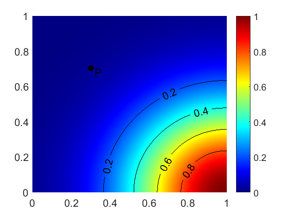
(a) $t_{1}$ = 0

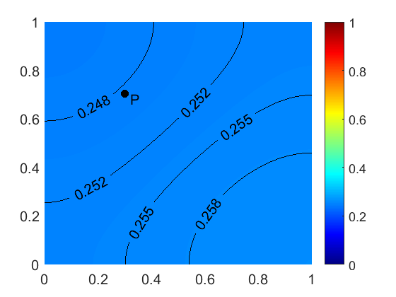
(b) $t_{2}$ = 0.5

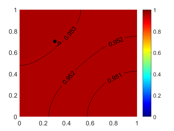
(c) $t_{3}$ = 2.5

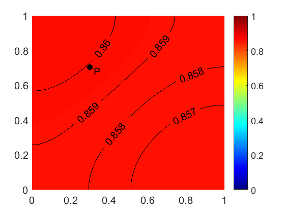
(d) $t_{4}$ = 7

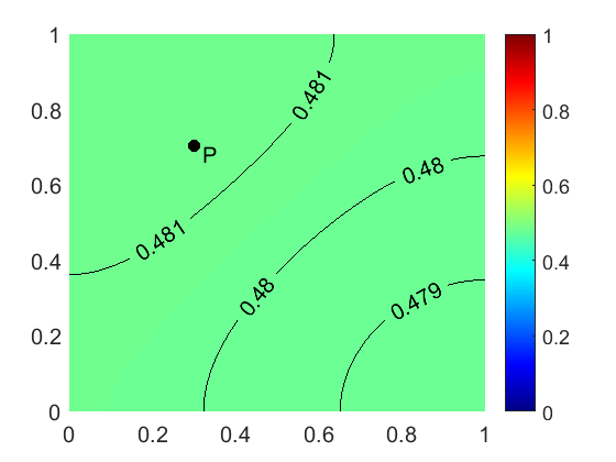
(e) $t_{5}$ = 10

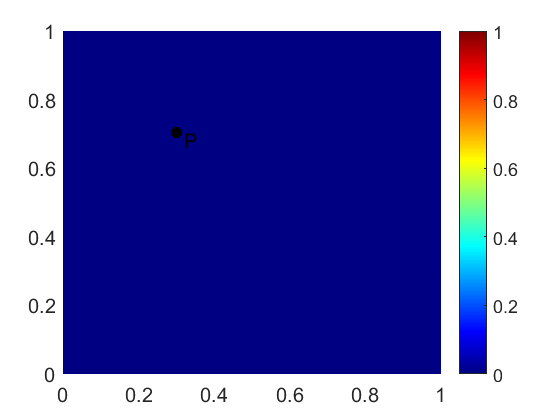
(f) $t_{6}$ = 14

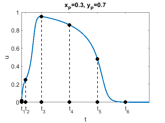
(g) Evolution at a specific point $P$

Figure 1: Snapshots of the evolution of the electrical potential. In Figures (a)-(f) the contour plots are shown in some selected instants $t_{1},\ldots,t_{6}$. Figure (g) reports the value of the electrical potential in a specific point $P$; the instants $t_{1},\ldots,t_{6}$ are remarked.

6.1 Spatial and temporal analysis

We now verify the validity of the estimates stated in Theorem 5.1. Due to the lack of an analytical expression for the solution of (2.1), we need to build a high-fidelity numerical solution $(\tilde{u},\tilde{w})$. In particular, we employ a reference fine mesh with $h_{ref}=4\cdot 10^{-3}$ and a time step $\tau_{ref}=2\cdot 10^{-3}$ to solve the Newton scheme (2.8)-(2.9), where $tol=10^{-15}$ is employed to make negligible the linearization error (see Remark 5.18). Employing $(\tilde{u},\tilde{w})$ it is possible to compute the error associated to different discrete solutions, obtained with different values of $h$ and $\tau$, and to assess the validity of the a posteriori error estimates introduced in Theorem 5.1 employing in particular the estimators defined in (5.18).

In Figure 2 we report the numerical verification of the upper bound (5.1) for two different choices of the discretization parameters $h$ and $\tau$. Each line is piecewise constant on every interval $(t_{n-1},t_{n})$. The red line represents the norm of the error on the interval $(0,t_{n})$ (see the left-hand side of (5.1) for its precise definition) computed with respect to the high-fidelity solution, whereas the blue line shows the sum of the estimators in each interval until $t_{n}$ (see the left-hand side of (5.1)). In this case the upper bound holds with constant $1$.

(a) $h=0.05$, $\tau=0.1$

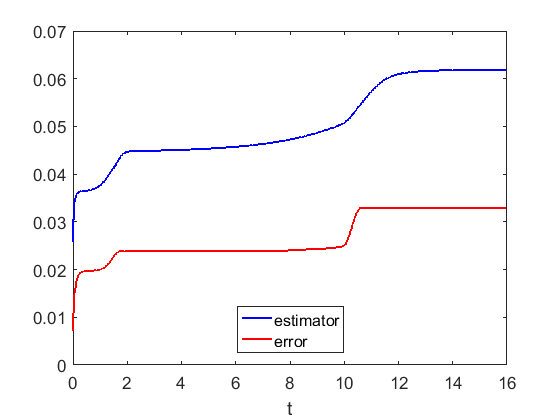
(b) $h=0.0125$, $\tau=0.025$

Figure 2: Assessment of the upper bound

Moreover, in Figure 3 we investigate the convergence rates for both the a posteriori estimator and the error norm with respect to the mesh size $h$ and the timestep $\tau$. The results are obtained by linearly reducing both $h$ and $\tau$ at the same time. The convergence history reported in Figure 3 shows that the error decays with linear rate, as expected from the a priori estimate in Theorem 3.3, and the a posteriori estimator decays with the same (linear) rate.

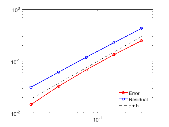
$h$	$\tau$	$tol$
$0.1$	$0.2$	$10^{-14}$
$0.05$	$0.1$	$10^{-14}$
$0.025$	$0.05$	$10^{-14}$
$0.0125$	$0.025$	$10^{-14}$
$0.00625$	$0.0125$	$10^{-14}$

Figure 3: Convergence analysis in $h$ and $\tau$

6.2 Linearization analysis

We now numerically assess the validity of the a posteriori estimate concerning the linearization error. In order to reduce as much as possible the numerical error induced by spatial and temporal approximations, we perform the the numerical experiments with the same discretization parameters ($h_{ref}=4\cdot 10^{-3}$, $\tau_{ref}=2\cdot 10^{-3}$) employed to build the high-fidelity numerical solution. Selecting an instant $t_{n}$, we compute several iterations of the Newton scheme (2.8)-(2.9) until the convergence criterion is satisfied with $tol=10^{-15}$. The iterative scheme produces a sequence $\{u_{h,K_{n}}^{n},w_{h,K_{n}}^{n}\}_{k=0,\ldots,K}$. Then, for each $k$ we compute $\gamma_{k}^{n}$ and compare it with the linearization error. In Figure 4 we report the described comparison at $t_{n}=2.5$ and $t_{n}=10$.

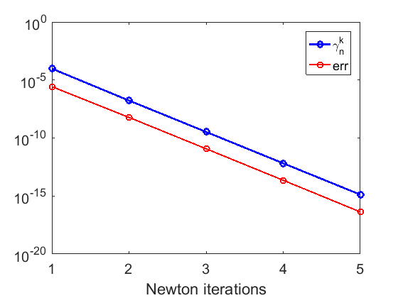
(a) $t_{n}=2.5$; accepted at iteration $5$

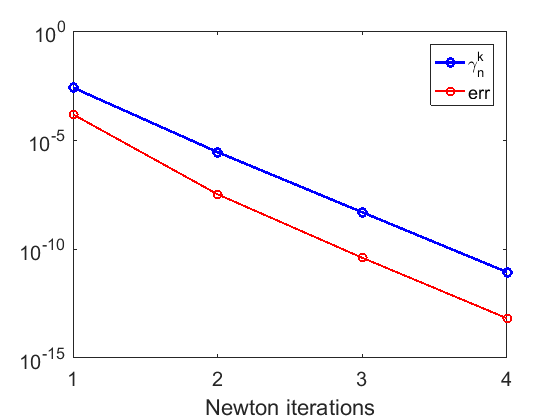
(b) $t_{n}=10$; accepted at iteration $4$

Figure 4: Assessment of the a posteriori indicator $\gamma_{k}^{n}$ for the linearization error

We observe that for each $k=1,\ldots,K$ the estimator is above the error, and they decrease with the same rate.

7 Conclusions

We considered the numerical approximation of the monodomain model, a system of a parabolic semilinear reaction-diffusion equation coupled with a nonlinear ordinary differential equation. The monodomain model arises from the (simplified) mathematical description of the electrical activity of the heart. In particular, we derived a posteriori error estimators accounting for different sources of error (space/time discretization and linearization). Moreover, after obtaining an a priori error estimate, we showed reliability and efficiency (this latter under a suitable assumption) of the error indicators. Lastly, a set of numerical experiments assess the validity of the theoretical results.

References

- [1] M. Amrein and T. P. Wihler “An adaptive space-time Newton-Galerkin approach for semilinear singularly perturbed parabolic evolution equations” In IMA J. Numer. Anal. 37.4, 2017, pp. 2004–2019
- [2] E. Beretta, C. Cavaterra and L. Ratti “Asymptotic expansion of boundary voltage perturbation in presence of small ischemic regions in the monodomain model of cardiac electrophysiology” In in preparation, 2018
- [3] E. Beretta, L. Ratti and M. Verani “Detection of conductivity inclusions in a semilinear elliptic problem arising from cardiac electrophysiology” In to appear in Commun. Math. Sci., 2018
- [4] Y. Bourgault, Y. Coudiere and C. Pierre “Existence and uniqueness of the solution for the bidomain model used in cardiac electrophysiology” In Nonlinear Anal Real World Appl 10.1 Elsevier, 2009, pp. 458–482
- [5] S. Brenner and R. Scott “The mathematical theory of finite element methods” Springer Science & Business Media, 2007
- [6] Z. Chen and J. Zou “Finite element methods and their convergence for elliptic and parabolic interface problems” In Numerische Mathematik 79.2 Springer, 1998, pp. 175–202
- [7] P. Clément “Approximation by finite element functions using local regularization” In Revue française d’automatique, informatique, recherche opérationnelle. Analyse numérique 9.R2 EDP Sciences, 1975, pp. 77–84
- [8] P. Colli Franzone et al. “Adaptivity in space and time for reaction-diffusion systems in electrocardiology” In SIAM J Sci Comput 28.3 SIAM, 2006, pp. 942–962
- [9] P. Colli Franzone, L.F. Pavarino and S. Scacchi “Mathematical Cardiac Electrophysiology” 13, MS&A Springer, 2014
- [10] P. Colli Franzone and G. Savaré “Degenerate evolution systems modeling the cardiac electric field at micro-and macroscopic level” In Evolution equations, semigroups and functional analysis Springer, 2002, pp. 49–78
- [11] A. Ern and M. Vohralík “Adaptive inexact Newton methods with a posteriori stopping criteria for nonlinear diffusion PDEs” In SIAM J Sci Comput 35.4 SIAM, 2013, pp. A1761–A1791
- [12] S. Sanfelici “Convergence of the Galerkin approximation of a degenerate evolution problem in electrocardiology” In Numer. Methods Partial Differential Equations 18.2 Wiley Online Library, 2002, pp. 218–240
- [13] S. Sanfelici “Numerical and analytic study of a parabolic-ordinary system modelling cardiac activation under equal anisotropy conditions” In Riv. Mat. Univ. Parma 5 5 Citeseer, 1996, pp. 143–157
- [14] J. Sundnes et al. “Computing the electrical activity in the heart”, Monographs in Computational Science and Engineering Series, Volume 1 Springer, 2006
- [15] V. Thomée “Galerkin finite element methods for parabolic problems” Springer, 1984
- [16] V. Thomée and L. Wahlbin “On Galerkin methods in semilinear parabolic problems” In SIAM Journal on Numerical Analysis 12.3 SIAM, 1975, pp. 378–389
- [17] R. Verfürth “A posteriori error estimates for finite element discretizations of the heat equation” In Calcolo 40.3 Springer, 2003, pp. 195–212
- [18] R. Verfürth “A review of a posteriori error estimation and adaptive mesh-refinement techniques” John Wiley & Sons Inc, 1996