Modelling the spinning dust emission from LDN 1780

Abstract

We study the anomalous microwave emission (AME) in the Lynds Dark Nebula (LDN) 1780 on two angular scales. Using available ancillary data at an angular resolution of 1 degree, we construct an SED between 0.408 GHz to 2997 GHz. We show that there is a significant amount of AME at these angular scales and the excess is compatible with a physical spinning dust model. We find that LDN 1780 is one of the clearest examples of AME on 1 degree scales. We detected AME with a significance $>20\sigma$. We also find at these angular scales that the location of the peak of the emission at frequencies between 23–70 GHz differs from the one on the 90–3000 GHz map. In order to investigate the origin of the AME in this cloud, we use data obtained with the Combined Array for Research in Millimeter-wave Astronomy (CARMA) that provides 2 arcmin resolution at 30 GHz. We study the connection between the radio and IR emissions using morphological correlations. The best correlation is found to be with MIPS 70 $\mu$m, which traces warm dust ($T\sim 50$ K). Finally, we study the difference in radio emissivity between two locations within the cloud. We measured a factor $\approx 6$ of difference in 30 GHz emissivity. We show that this variation can be explained, using the spinning dust model, by a variation on the dust grain size distribution across the cloud, particularly changing the carbon fraction and hence the amount of PAHs.

1 Introduction

The WMAP (Bennett et al., 2013) and Planck (Planck Collaboration et al., 2011b) satellites, as a byproduct of the making of Cosmic Microwave Background (CMB) maps, have provided precise full-sky maps of the different diffuse emission mechanisms on the Galaxy. Among them is the anomalous microwave emission (AME), first detected by Leitch et al. (1997) as a correlation between dust emission at 100$\,\mu\mathrm{m}$ from IRAS and 14.5 GHz radio emission toward the north celestial pole, that could not be accounted for by synchrotron or free-free emission.

In our Galaxy, AME can account for up to 30% of the diffuse emission at 30 GHz (Planck Collaboration et al., 2016b, d). AME has been observed in different astrophysical environments, such as molecular clouds (Finkbeiner et al., 2002; Watson et al., 2005; Casassus et al., 2006, 2008; AMI Consortium et al., 2009; Dickinson et al., 2010), translucent clouds (Vidal et al., 2011), reflection nebulae (Castellanos et al., 2011), Hii regions (Dickinson et al., 2007, 2009; Todorović et al., 2010) and in the galaxies NGC 6946 and NGC 4725 (Murphy et al., 2010, 2018). AME may also be important in compact objects like protoplanetary disks (PPDs). Hoang et al. (2018) predicted that AME from spinning silicates or polycyclic aromatic hydrocarbons (PAHs) dominates over thermal dust emission at frequencies $<60$ GHz in PPDs, even in the presence of significant dust growth and Greaves et al. (2018) reproduced the EME they detect in two disks using a model in which hydrogenated nanodiamonds were the spinning carriers. For an up to date review on AME, refer to Dickinson et al. (2018).

AME is the least-understood emission mechanism in the 1 – 100 GHz range. It is difficult to study AME due to its diffuse nature, being clearly detected by CMB experiments and telescopes at $\sim 1$ degree angular resolution but difficult to detect at higher angular resolutions (although there are well known regions were it has been observed with high resolution, e.g. Scaife et al., 2010; Tibbs et al., 2011; Battistelli et al., 2015). This presents a problem for the identification of the emitters and their physical properties so, at the moment, we only know some general properties of AME, like being associated with photodissociation regions (PDRs). AME is thought to be caused by dust grains, possessing electric dipole moments, spinning at GHz frequencies. This is an old idea that was first proposed by Erickson (1957).

The spinning dust (SD) hypothesis has been preferred by the observations and the more convincing examples are the Perseus and $\rho$ Ophiuchi molecular clouds (Watson et al., 2005; Casassus et al., 2008; Planck Collaboration et al., 2011c). Currently, detailed theoretical models have been constructed that predict the SD spectrum for different grain types and astrophysical environments (Draine & Lazarian, 1998; Ali-Haïmoud, Hirata & Dickinson, 2009; Hoang, Draine & Lazarian, 2010; Silsbee, Ali-Haïmoud & Hirata, 2011; Ysard, Juvela & Verstraete, 2011; Hoang & Lazarian, 2012). They present an opportunity to study the ISM, in particular the smallest dust grains, from a new window at GHz frequencies. Spinning dust emission depends on factors such as the gas density, temperature, ionization fraction and grain size distribution, so the detailed comparison of the models with good observations will allow us to study the ISM conditions in a variety of environments.

Nevertheless, some doubt has been cast on the SD paradigm by (Hensley, Draine & Meisner, 2016), who found that the Planck AME map is uncorrelated with a template of PAH emission. PAH are thought to be one of he main carriers of AME in the SD model. This shows that much research is still needed in this area.

Here we present 30 GHz data from the Combined Array for Research in Millimeter-wave Astronomy (CARMA) of the Lynds Dark Nebula (LDN) 1780, a high Galactic latitude (l = 359^∘​​.0, b = 36^∘​​.7) translucent region at a distance of 110$\pm$10 pc (Franco, 1989). LDN 1780 has a moderate column density (a few $\times 10^{21}$ cm^-2) that corresponds to the “translucent cloud” type of object, i.e. interstellar clouds with some protection from the radiation field, with optical extinctions in the range $A_{V}\sim 1-4$ mag (Snow & McCall, 2006). Using an optical-depth map constructed from ISO 200 $\mu$m observations, Ridderstad et al. (2006) found a mass of $\sim$ 18 M_⊙ and reported no young stellar objects based on the absence of colour excess in point sources.

LDN 1780 is a known source of AME. Vidal et al. (2011) detected AME from this cloud through observations at 31 GHz. They found that the AME at 30 GHz correlates best with the IRAS 60 $\mu$m map, which traces hot and small dust grains. This correlation was even tighter than with an 8 $\mu$m, which traces PAH. Here we revisit this cloud, using archival data to study the spectral energy distribution (SED) at 1 degree angular scales. We also use our CARMA data in addition to IR and sub-mm templates to study and model the AME on angular scales of 2 arcmin.

In Section 2 we describe the CARMA observations, as well as the ancillary data used in the analysis. Section 3 describes the SED of the cloud on 1 deg angular scales. Section 4 correspond to the analysis at 2 arcmin resolution based on the CARMA data. Section 5 concludes.

2 Data

2.1 CARMA data

We obtained 31 GHz data from the Combined Array for Research in Millimeter-wave Astronomy (CARMA). It consists of 8 antennas of 3.5 m diameter. Six “inner” telescopes are arranged in a compact configuration, with baselines ranging from 4.5 to 11.5 m. The two other telescopes provide baselines of 56 and 78 m. The receivers observe the frequency range 26–36 GHz in total intensity. The primary beam corresponds to $\approx 11^{\prime}$ at 31 GHz.

We prepared a three pointings mosaic observation centred at the peak of the cloud at 31 GHz as observed by the Cosmic Background Imager (CBI) in Vidal et al. (2011), and also, to include the “gradient” of IR emission, i.e. regions where the morphology of the different IR maps differs. In Fig. 1 we show the three pointing mosaic, overlaid on top of the CBI image of the cloud, from Vidal et al. (2011).

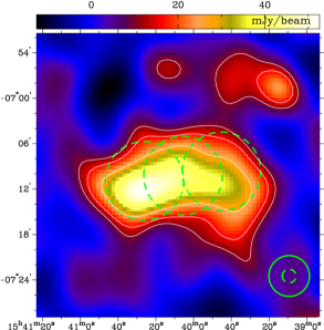
Figure 1: Mosaic pointings of the CARMA observations. The colour image shows the emission at 31 GHz as seen by the CBI (Vidal et al., 2011), with a peak of 53 mJy/beam and a synthesised beam of 5.4 arcmin. The dashed circles along the cloud show the location of the three pointings where we observed the cloud with CARMA, with the size of them indicating the primary beam of the CARMA antennas of 10.5 arcmin. At the bottom-right corner are shown the synthesised beam sizes for the CBI (5.4 arcmin) and CARMA (inner, 1.8 arcmin).

2.2 Observations and calibration

The observations were performed in two runs, first between 2012-06-09 and 2012-07-21 and, and between 19-05-2013 and 14-06-2013. Each run is divided into small observations blocks (OB). The total observing time adds up to 25.2 hours (or 4 sidereal passes) of telescope time. During each one of the OB, the source is observed along with three calibrators, namely flux calibrator (3C273), passband calibrator (1337-129) and phase calibrator (1512-090). The OB consisted on observations of the flux calibrator during 5 min, then observation of the passband calibrator during 5 min, followed by the target cycle where the phase calibrator is observed during 3 m, followed by 15 on source.

We calibrated the data using the Miriad data-reduction package (Sault, Teuben & Wright, 1995). We performed a small amount of flagging to remove particularly noise combinations of baselines and spectral channels.

2.3 Imaging

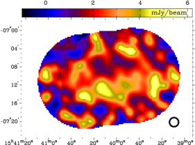
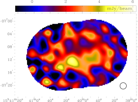
Figure 2: Clean (top) and MEM (bottom) mosaic reconstructions of the data after the $uv$ tapering, in order to increase the SNR of the extended emission. The angular resolution in this case is 2^′ for both maps. The r.m.s. noise value of the CLEAN map is 1.4 mJy beam^-1​, and the noise of the MEM map is 0.99 mJy beam^-1​.

To image the calibrated visibilities, we tried both CLEAN (e.g. Högbom, 1974) and MEM (e.g. Cornwell & Evans, 1985) reconstructions. This was done to identify any possible imaging artifact of the extended emission. We used natural weights in order to maximize the S/N in the restored image.

Two radio sources from the Condon et al. (1998) catalogue are visible in the maps. They are listed in Table 1. We subtracted these sources from the visibilities, as we are only interested in the diffuse emission from the cloud. We did this by first using CLEAN to obtain their flux density. An appropriate point model is then subtracted from the visibilities. Table 1 also lists our measured coordinates and flux densities at 31 GHz. We inspected the subtracted maps after to check for artifacts in case of a bad estimation of the flux. Any residual from the source subtraction is smaller than the r.m.s noise of the maps.

Table 1: Point sources subtracted from the visibilities. The location and 1.4 GHz fluxes are from the Condon et al. (1998) catalogue. The 31 GHz fluxes were obtained from our CARMA observations.

NVSS name	$S_{1.4\,{\rm GHz}}$	$S_{31\,{\rm GHz}}$	$\alpha_{1.4/31}$
	mJy	mJy
J154006-070442	$25.8\pm 1.3$	$3.5\pm 1.2$	$-0.64\pm 0.26$
J154024-070858	$13.3\pm 0.6$	$6.2\pm 1.3$	$-0.25\pm 0.16$

In order to increase the sensitivity to extended emission, we use Gaussian $(u,v)$ tapering. This is the multiplication of the visibilities with a Gaussian filter which has the effect of down-weighting the longer baselines, degrading the final angular resolution of the map and increasing the S/R of the more extended emission. The original angular resolution of the map using natural weights is $\sim 1^{\prime}$​​.$6$. We used a filter size in the Fourier space equivalent to a Gaussian smoothing kernel in the image plane which produces a final map with 2^′ resolution. An added advantage of smoothing CARMA data to 2 arcmin resolution is that it symmetrises the beam.

After imaging with both methods, CLEAN and MEM, the r.m.s. noise in the CLEAN map is 40% larger than the noise in the MEM map (1.4 mJy beam^-1 and 0.99 mJy beam^-1 respectively). In Fig. 2 we show the two maps. The synthesised beam size is plotted as an ellipse at the bottom-right corner. It has a size of $2^{\prime}$ FWHM. Both maps present a similar morphology, but the MEM reconstruction seem to recover more of the diffuse and extended flux. We use the MEM map for the rest of the analysis due to this and its lower noise value.

2.4 Ancillary data

Besides the CARMA data, we also used ancillary data to study the cloud. We used radio and IR data to build an SED of LDN 1780 from 0.408 GHz to 2997 GHz on a 1^∘ scale. Table 2 lists all the data used.

Table 2: List of ancillary data used in the analysis.

Telescope/Survey	Freq. [GHz]	Nominal Resolution	Reference
Haslam	0.408	56’$\!\!.$0	Haslam et al. (1982); Remazeilles et al. (2015)
Reich	1.42	35’$\!\!.$4	Reich (1982); Reich & Reich (1986); Reich, Testori & Reich (2001)
Jonas	2.3	20’$\!\!.$0	Jonas, Baart & Nicolson (1998)
WMAP  9-year	22.8	51’$\!\!.$3	Bennett et al. (2013)
Planck	28.4	32’$\!\!.$3	Planck Collaboration et al. (2016a)
WMAP  9-year	33.0	39’$\!\!.$1	Bennett et al. (2013)
WMAP  9-year	40.7	30’$\!\!.$8	Bennett et al. (2013)
Planck	44.1	27’$\!\!.$1	Planck Collaboration et al. (2016a)
WMAP  9-year	60.7	21’$\!\!.$1	Bennett et al. (2013)
Planck	70.4	13’$\!\!.$3	Planck Collaboration et al. (2016a)
WMAP  9-year	93.5	14’$\!\!.$8	Bennett et al. (2013)
Planck	100	9’$\!\!.$7	Planck Collaboration et al. (2016a)
Planck	143	7’$\!\!.$3	Planck Collaboration et al. (2016a)
Planck	217	5’$\!\!.$0	Planck Collaboration et al. (2016a)
Planck	353	4’$\!\!.$8	Planck Collaboration et al. (2016a)
Planck	545	4’$\!\!.$7	Planck Collaboration et al. (2016a)
Planck	857	4’$\!\!.$3	Planck Collaboration et al. (2016a)
COBE-DIRBE	1249	37’$\!\!.$1	Hauser et al. (1998)
COBE-DIRBE	2141	38’$\!\!.$0	Hauser et al. (1998)
COBE-DIRBE	2997	38’$\!\!.$6	Hauser et al. (1998)

We used the re-processed version of the 0.408 GHz map of Haslam et al. (1982) by Remazeilles et al. (2015) available at the LAMBDA website. It has an effective resolution of 56^′ and includes all the point sources. At 1.42 GHz the Reich et al. map (Reich, 1982; Reich & Reich, 1986; Reich, Testori & Reich, 2001) has an angular resolution of 36^′. The 2.326 GHz map from Jonas, Baart & Nicolson (1998) has an angular resolution of 20’$\!\!.$  We assumed a 10% uncertainty in these three data sets. An additional uncertainty of 0.8 K is added to the 0.408 GHz map, in order to account for the striations on the map as measured in Remazeilles et al. (2015).

We included the five WMAP 9-yr maps (Bennett et al., 2013), from 23 to 94 GHz, smoothed to 1^∘ ​​. We assumed a conservative 4% uncertainty (the calibration uncertainty quoted in Bennett et al., 2013, is 0.2%). This is to account for any additional uncertainty due to non-symmetric beams, and any colour correction effect, as the spectral index of the source is not equal to the CMB spectrum.

We also include Planck data. Planck observes the full sky in nine frequency bands between 28 and 857 GHz. We used the temperature maps which were released in 2015 (PR2), described in Planck Collaboration et al. (2016a) and are available in the Planck Legacy Archive.

3 SED at 1^∘ resolution

3.1 Flux densities measurement

To obtain the flux densities of the cloud at the different frequencies, the maps that are originally in antenna temperature units, are expressed in flux units (Jy pixel^-1) using the relation,

$$S=\frac{2\,k\,T_{RJ}\,\nu^{2}\,\Omega_{\mathrm{pix}}}{c^{2}},$$ (1)

where $\Omega_{\mathrm{pix}}$ is the solid angle of each pixel, $T_{RJ}$ the brightness temperature, $\nu$ the observing frequency, $k$ the Boltzmann constant and $c$ the speed of light (see Planck Collaboration et al., 2011c, 2014c, for a similar analysis on other sources).

The flux densities are measured by integrating the flux density over a 2^∘ diameter aperture, centred at the position of the cloud. We subtract the background level using the median value of the pixels that lie in an annular aperture between 80^′ and 100^′ from the position of the source. The r.m.s. variations in this ring are used to estimate the uncertainty in the measured fluxes, including noise, CMB and background variations.

In Fig. 3 we present the 20 maps we used of LDN 1780, from 0.408 GHz up to 2997 GHz. All of them have been smoothed to a common 1^∘ resolution. Each image is 5^∘ on a side and the circular aperture and ring used for the photometry are indicated. The cloud is clearly visible in the high frequency maps, from 217 GHz, where the thermal dust emission dominates above the diffuse background. At lower frequencies, between 23 and 143 GHz, all the maps show a similar structure, the CMB fluctuations that predominate over this frequency range and angular scales. At even lower frequencies, in the 0.408, 1.4 and 2.3 GHz maps, there is no emission from the region of the cloud visible above the background.

A main goal of the Planck and WMAP mission was to produce an accurate map of the CMB fluctuations. We use the SMICA CMB map (Planck Collaboration et al., 2016c) to subtract the CMB anisotropy from the individual frequency maps. By doing this, LDN 1780 cloud is recognisable above the background in all the maps between 23 and 2997 GHz. Fig. 4 show these CMB-subtracted maps. In them, LDN 1780 is easily discernible. The peak position of the source varies slightly among some of the maps (e.g. WMAP 23 GHz, Planck 545 GHz). We will discuss this in Sect. 3.3.

Additional structure can be seen around LDN 1780 at the 40–92 GHz CMB subtracted maps in Fig. 4. We measured the standard deviation of these fluctuations around the cloud in the three mentioned maps, using a ring with an inner radius of 1^∘ ​ centred at the location of LDN 1780, and a thickness of 3^∘​. We compared the standard deviation within the ring with the r.m.s. noise of each map in the same ring. The r.m.s. noise was calculated using 500 simulations of pure noise for each map, constructed using the variance maps provided by the WMAP and Planck collaborations. Table 3 lists the standard deviation values around LDN 1780 in the Planck-44 GHz, WMAP-60 GHz and Planck-70 GHz CMB subtracted maps, as well as the r.m.s. noise values of each of those data sets. The r.m.s. noise values can account for at least 50% of the measured fluctuations around LDN 1780. The additional residual fluctuations are a combination between uncertainties in the CMB map and additional diffuse foregrounds fluctuations. We measured the mean standard deviation between four different CMB maps provided by the Planck collaboration: Commander, , NILC, SEVEM and SMICA (Planck Collaboration et al., 2016c). In the same aperture, the fluctuations between these maps average a value of 5.6 $\mu$K. This value can be used as a measurement of the uncertainty of the CMB map in this region. This noise in the CMB map, in addition with the r.m.s. noise value of the maps can account for the measured fluctuations around LDN 1780.

Table 3: Standard deviation of the fluctuations visible around LDN 1780 in three of the CMB subtracted maps from Fig. 4. They are measured within a ring centred at the cloud, with an inner radius of 1^∘ and an outer radius of 3^∘ ​​. The second column shows the r.m.s. noise values measured in the same ring.

Map	Standard deviation	r.m.s. noise
	$\mu$K	$\mu$K
Planck  44 GHz	$12.0$	$5.9$
WMAP  60 GHz	$7.6$	$4.7$
Planck  70 GHz	$7.0$	$4.3$

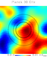
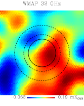
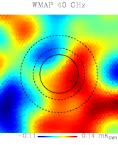
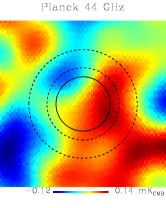
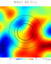
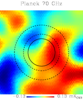
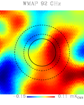
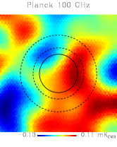
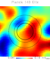
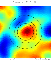
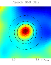
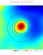
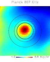
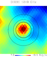
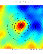
Figure 3: Maps of LDN 1780 at different frequencies ranging from the Haslam et al. map at 0.408 GHz to the DIRBE image at 2997 GHz. The square maps have 5^∘ in side and all have been smooth to a common angular resolution of 1^∘ FWHM. The colour scale is linear, ranging from the minimum to the maximum of each map. The inner circle shows the aperture where we measured the flux and the dashed larger circles show the annulus used to estimate the background emission and noise around the aperture.

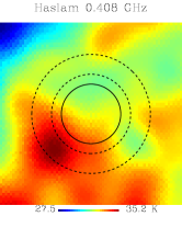
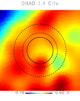
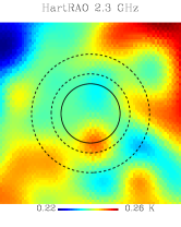
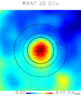
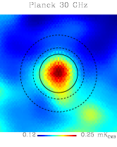
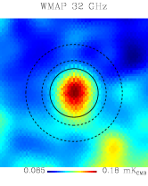
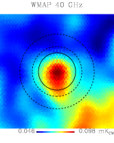
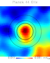
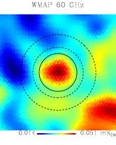
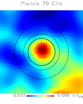
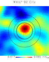
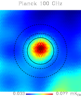
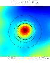
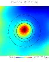
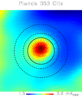
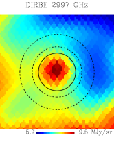
Figure 4: CMB-subtracted maps of LDN 1780 at different frequencies ranging from the Haslam et al. map at 0.408 GHz to the DIRBE image at 2997 GHz. The square maps have 5^∘ in side and all have been smooth to a common angular resolution of 1^∘ FWHM. The colour scale is linear, ranging from the minimum to the maximum of each map. The inner circle shows the aperture where we measured the flux and the dashed larger circles show the annulus used to estimate the background emission and noise around the aperture. Compare these CMB-subtracted maps with the original ones shown in Fig. 3, in particularly between 23 and 217 GHz, where the CMB anisotropy dominates.

In Table 4 we list the flux densities measured using the aperture photometry. We also list the values for the flux densities measured in the CMB-subtracted map. The fluxes measured at the three lowest frequencies were negative, i.e. the background level in the ring is larger than the flux in the aperture. Because of this, we give a $2\,\sigma$ upper limit for each one of these points. In the next section we describe the SED fitting to the values listed in Table 4.

Table 4: Flux densities of LDN 1780over a 2^∘ diameter aperture.

Survey	Frequency	Flux density	CMB-sub flux density
	[GHz]	[Jy]	[Jy]
Haslam	0.4	$<2.2$	$<2.2$
DRAO	1.4	$<0.14$	$<0.14$
HartRao	2.3	$<0.12$	$<0.12$
WMAP	23	$1.4\pm 0.05$	$1.1\pm 0.06$
$Planck$	30	$1.6\pm 0.09$	$1.1\pm 0.07$
WMAP	33	$1.3\pm 0.10$	$0.8\pm 0.08$
WMAP	41	$1.4\pm 0.16$	$0.8\pm 0.11$
$Planck$	44	$1.5\pm 0.18$	$0.8\pm 0.12$
WMAP	61	$1.7\pm 0.33$	$0.7\pm 0.22$
$Planck$	70	$2.8\pm 0.42$	$1.4\pm 0.27$
WMAP	93	$3.9\pm 0.70$	$1.7\pm 0.48$
$Planck$	100	$5.5\pm 0.72$	$3.0\pm 0.45$
$Planck$	143	$10.8\pm 1.1$	$6.5\pm 0.79$
$Planck$	217	$33.8\pm 1.4$	$27.8\pm 1.6$
$Planck$	353	$123\pm 2$	$124\pm 4$
$Planck$	545	$407\pm 10$	$407\pm 13$
$Planck$	857	$1151\pm 31$	$1151\pm 40$
DIRBE	1249	$1860\pm 62$	$1860\pm 81$
DIRBE	2141	$1639\pm 83$	$1639\pm 108$
DIRBE	2997	$749\pm 35$	$749\pm 46$

3.2 SED fitting

SEDs in this frequency range are usually modeled using five components, namely synchrotron, free-free, AME, CMB and thermal-dust emission. In this case, we do not include a synchrotron component, due to the small flux densities measured at the lower frequency bands. Our model for the flux densities in a 2^∘ aperture is therefore described by four components,

$$S=S_{ff}+S_{AME}+S_{CMB}+S_{TD}.$$ (2)

The free-free level in LDN 1780 itself is very low. The H$\alpha$ line can be used as a tracer of free-free emission provided that the line is the result of in situ recombination. There is some H$\alpha$ emission coming from the cloud but Witt et al. (2010) showed that most of it consists of scattered light from the diffuse H$\alpha$ component of the galactic interstellar radiation field (ISRF). We include a conservative upper limit for the free-free component in the SED fitting, using the estimation at 31 GHz over a 1^∘ scale of $S_{31}=0.09$ Jy from Vidal et al. (2011), that was calculated using the H$\alpha$ map from the SHASSAA survey (Gaustad et al., 2001).

We extrapolate this value to lower and higher frequencies using a power law with the form,

$$S_{ff}=S_{31}\,(\nu/31\,\mathrm{GHz})^{\beta_{ff}},$$ (3)

where $\alpha_{ff}=-0.13$ is the free-free spectral index (for flux density) valid for the diffuse ISM (Draine, 2011).

The AME component is accounted for using a spinning dust model, provided by the SPDUST package (Ali-Haïmoud, Hirata & Dickinson, 2009; Silsbee, Ali-Haïmoud & Hirata, 2011). This program calculates the emissivity, $j_{\nu}$, in terms of the hydrogen column density of a population of spinning dust grains. It requires a number of physical parameters to generate the spectrum. We used the ideal description for the “warm neutral medium” (WNM) as defined by Draine & Lazarian (1998). The generated spectrum produces peaks at 23.6 GHz. We fit for the amplitude of this generic spectrum, so this component in the SED has only one free parameter, $A_{sd}$. In Section 4.2 we describe in more detail the SPDUST modelling.

A CMB component is included, using the differential form of a blackbody at $T_{\mathrm{CMB}}=2.726\,\mathrm{K}$ (Fixsen, 2009). The flux density of this component has the form

$$S_{\mathrm{CMB}}=\left(\frac{2\,k\,\nu^{2}\,\Omega}{c^{2}}\right)\Delta\mathrm{T_{\mathrm{CMB}}},$$ (4)

where $\Delta\mathrm{T_{\mathrm{CMB}}}$ is the CMB anisotropy temperature, in thermodynamics units.

The dust emission at wave lengths $\lambda>60$ $\mu$m is usually described using a modified blackbody model. The flux density measured in a solid angle $\Omega$ is,

$$S_{TD}=2\,h\,\frac{\nu^{3}}{c^{2}}\frac{1}{e^{h\nu/kT_{d}}-1}\,\tau_{250}(\nu/1.2\,\mathrm{THz})^{\beta_{d}}\,\Omega,$$ (5)

where $k$, $c$ and $h$ are the Boltzmann constant, the speed of light and the Planck constant respectively; $T_{d}$ is the dust temperature and $\tau_{250}$ is the optical depth at $250\,\mu$m.

We used the MPFIT IDL package (Markwardt, 2009), which uses the Levenberg–Marquardt algorithm to calculate a non-linear least-squares fit. There are two Planck bands, centered at 100 GHz and at 217 GHz, which can include a significant amount of CO line emission (Planck Collaboration et al., 2014b), corresponding to the transitions $J$=1$\rightarrow$0 at 115 GHz and $J$=2$\rightarrow$1 at 230 GHz. LDN 1780 is known to have a molecular component (Laureijs et al., 1995). To avoid contamination from these lines in the fluxes measured at these bands, we did not include these two channels in our fit.

In the top panel of Fig. 5 we show the best fit to the data while the bottom panel shows the best fit to the CMB-subtracted data. In both plots, the low frequency data are represented with $2\sigma$ upper limits. The largest uncertainty at 0.408 GHz comes from the $\pm 0.8$ K striations measured by Remazeilles et al. (2015). The blue triangle at 23 GHz represents the expected free-free level predicted by the WMAP MEM map (Bennett et al., 2013). A small CO contribution can be seen at 100 GHz and at 217 GHz in the CMB-subtracted SED, however its flux is less than 10% at 100 GHz. Being such at small effect at 100 and 217 GHz means that it will be negligible at 353 GHz, so it is safe that we have use the 353 GHz map in our SED. In Table 5 we list the parameters and uncertainties derived from the fit.

Table 5: Fitted parameters for the SED of LDN 1780. Also listed is the reduced $\chi^{2}$ of the fit. The second column lists the parameters of the fit using the CMB-subtracted maps.

Parameter	Normal	No–CMB
$\tau_{250}[\times 10^{-5}]$	$2.1\pm 0.2$	$2.2\pm 0.3$
Td [K]	$17.1\pm 0.4$	$16.9\pm 0.5$
$\beta_{d}$	$1.5\pm 0.1$	$1.5\pm 0.1$
A${}_{sd}[10^{20}\,\mathrm{cm}^{-2}]$	$2.4\pm 0.1$	$2.0\pm 0.1$
$\Delta T_{\mathrm{CMB}}$ [$\mu$K]	$13.3\pm 1.7$	$2.3\pm 1.3$
$\chi^{2}_{r}$	0.9	1.9

The difference in the fitted parameters between the CMB-subtracted data and the un-subtracted maps is small and consistent with zero within the uncertainties. The CMB component fitted in the CMB-subtracted maps is consistent with zero. The fact that the measured $\Delta T_{\mathrm{CMB}}=0.5\pm 0.4\,\mu$K is consistent with zero shows consistency within the two fits. The $\chi^{2}_{r}$ is higher when using the CMB-subtracted maps. A reason for this is that the error bars of the data points in this case are smaller, because the fluctuations in the annular aperture are much smaller after subtracting the CMB anisotropy. In this cloud, the CMB contribution is significant on scales $\sim 1^{\circ}$, but we show that it is well quantified.

These SEDs show that there is significant AME present in this cloud. If we assume the spinning dust component of the fit to be zero, the overall CMB-subtracted fit is extremely poor, giving a $\chi^{2}_{r}=40$, compared with the case when we include the spinning dust component ($\chi^{2}_{r}=40$). The amplitude of the spinning dust component is A${}_{sd}=2.4\pm 0.1$ and A${}_{sd}=2.0\pm 0.1$ for the original and CMB-subtracted maps respectively. This corresponds to a significance of 24$\sigma$ and 20$\sigma$ respectively, making LDN 1780 one of the clearest examples of AME on 1^∘  angular scales. In the analysis by Planck Collaboration et al. (2014c), LDN 1780 was not detected as an AME source. We believe that the reason is that LDN 1780 does not appear as a conspicuous source in the original maps, and only shows clearly after subtracting a CMB template, as its location is coincident with a high value of the CMB anisotropy.

Another important aspect to highlight is the lack of emission from the cloud in the low-frequency maps ($\nu\leq 2.3$ GHz). This means that LDN 1780 is a rising spectrum source at $\nu>5$ GHz.

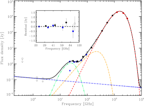
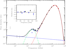
Figure 5: Spectra of LDN 1780 including low frequency data, WMAP (blue dots), Planck (black dots) and COBE-DIRBE data (red dots). The black line is the best fit to the data, which includes four components. Thermal dust emission is represented with a red dashed line. A CMB component is shown in orange. The blue line represent an upper limit for the free-free emission as expected from the H$\alpha$ map. The blue triangle shows the free-free emission expected from the WMAP 9-yr MEM template. The green line represents the spinning dust model. The two points that can be contaminated by CO line emission, at 100 GHz and at 217 GHz, are shown as a empty black circle. The fits do not include a synchrotron component. The insert shows the residuals (data–model) around the region where the spinning dust component is important. The residuals are consistent with zero. The bottom panel shows the SED constructed using the CMB-subtracted maps.

3.3 Peak location

If we take a closer look to Fig. 4, we can notice that the location of the peak of the cloud in the lower frequencies (23–70 GHz) is very close to the center of the aperture. On the other hand, the cloud appears shifted north by a few arcmin in the higher frequency maps (93–2997 GHz). In order to measure this shift, we measured the position of the peak of the cloud in all the maps from 23 to 2997 GHz using sextractor (Bertin & Arnouts, 1996). Table 6 list the location and uncertainties for the peak of the emission for all the maps between 23 and 2997 GHz. In Fig. 6 we plot these values using coloured ellipses on top of the 250 $\mu$m Herschel map orientated in Galactic coordinates, where the blue ellipses correspond to the maps from 22.8 GHz to 60.7 GHz, and the red ellipses to the maps from 70.4 GHz to 2997 GHz. The averaged position is also plotted for as a filled ellipse.

The location of the low-frequency (22.8–60.7 GHz) peak is closer to the peak of the IR emission originated from small grains (e.g. 8 $\mu$m, 12 $\mu$m). This is most interesting as it is what is expected from the spinning dust model. Moreover, this is also along the direction of the local radiation field that illuminates the cloud, which comes from the Galactic plane direction (Witt et al., 2010). We will explore further this morphological correlation using the CARMA data in the next Section.

Table 6: Location of the peak of the cloud for WMAP, Planck and DIRBE maps in Galactic coordinates. We also list the averaged values for the maps in the range 70.4–2997 GHz and 22.8–60.7 GHz.

Map	Gal. Lon. [deg]	Gal. Lat. [deg]
DIRBE 2997	$359.19\pm 0.02$	$36.63\pm 0.02$
DIRBE 2141	$359.17\pm 0.02$	$36.67\pm 0.01$
DIRBE 1249	$359.17\pm 0.02$	$36.61\pm 0.02$
Planck 857	$359.17\pm 0.02$	$36.62\pm 0.02$
Planck 545	$359.18\pm 0.03$	$36.63\pm 0.03$
Planck 353	$359.17\pm 0.03$	$36.63\pm 0.03$
Planck 217	$359.17\pm 0.07$	$36.63\pm 0.06$
Planck 143	$359.16\pm 0.13$	$36.61\pm 0.13$
Planck 100	$359.13\pm 0.15$	$36.60\pm 0.15$
WMAP 93.5	$359.07\pm 0.19$	$36.76\pm 0.17$
Planck 70.4	$359.10\pm 0.19$	$36.35\pm 0.25$
Averaged	$359.077\pm 0.002$	$36.635\pm 0.002$
WMAP 60.7	$359.22\pm 0.22$	$36.48\pm 0.17$
Planck 44.1	$359.16\pm 0.15$	$36.46\pm 0.17$
WMAP 40.7	$359.12\pm 0.12$	$36.16\pm 0.17$
WMAP 33	$359.05\pm 0.08$	$36.41\pm 0.11$
Planck 28.4	$359.13\pm 0.08$	$36.42\pm 0.08$
WMAP 22.8	$359.11\pm 0.05$	$36.44\pm 0.07$
Averaged	$359.13\pm 0.04$	$36.43\pm 0.05$

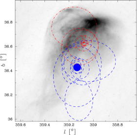
Figure 6: Ellipses centred at the location of the peak of the cloud for the WMAP, Planck and DIRBE maps. The size of the ellipses represent 1-$\sigma$ uncertainties, taken from Table 6. In blue are shown the frequencies between 22.8 GHz and 60.7 GHz while in red the maps from 70.4 to 2997 GHz. The filled ellipses correspond to the averaged values shown also in Table 6. On grey scale is the 250 $\mu$m Herschel map of LDN 1780 in Galactic coordinates.

4 Dust properties at 2^′ resolution

Using the IR data available at angular resolutions similar to our CARMA maps of 2^′, we can obtain some physical properties of the cloud, such as its temperature and column density. We do this by fitting for the spectrum of the thermal dust emission (as defined in Eq. 5) in each pixel. For this fit, we use five data points, at 70, 160, 250, 350, and 500$\,\mu\mathrm{m}$, which are dominated by thermal dust.

Due to the smaller number of data points that we have here in comparison to the previous fit at 1^∘ scales (5 versus 20), we fix the dust spectral index to $\beta_{d}=1.6$, a value similar to the one measured in the 1^∘ fit, and also, consistent with the values for the diffuse medium measured by Planck (Planck Collaboration et al., 2014a). This means that in this case our modified black-body fit only has two parameters, the optical depth $\tau_{250}$ and the temperature of the big grains. We have calculated the fit only where the signal-to-noise ratio of the pixels is larger than 2. In Fig. 7 we show the resulting map for the optical depth at 250$\,\mu\mathrm{m}$ and for the temperature of the dust. The colder regions corresponds to where the optical depth is larger. This is expected as these regions are more shielded from the ISRF.

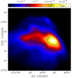
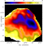
Figure 7: Map of optical depth at 250$\,\mu\mathrm{m}$ (left) and the dust temperature (right) for LDN 1780. The coldest areas of the cloud, at $T_{d}\approx 14$ K correspond to regions with larger optical depth. This is expected as the denser regions are more shielded from the radiation field.

From the optical depth map, we can obtain a hydrogen column density map using the linear relation $\tau_{250}/N_{H}=2.32\pm 0.3\times 10^{-25}$ cm², as measured by Planck Collaboration et al. (2011a). From the temperature map, we can derive a map for the radiation field. The radiation field $G_{0}$ can be estimated using the following relation (Ysard, Miville-Deschênes & Verstraete, 2010),

$$G_{0}=\left(\frac{T_{d}}{17.5\,[\mathrm{K}]}\right)^{\beta_{d}+4},$$ (6)

where the spectral distribution of the radiation field is assumed to have the standard shape, defined in Mathis, Mezger & Panagia (1983). Planck Collaboration et al. (2014a) has shown that this relation might not hold in every environment, and variations in $T_{d}$ might be due to variations in dust properties, such as grain structure or size distribution. We will use this map in the following Section.

4.1 IR correlations

Here we investigate correlations with the IR data. We include the Spitzer-IRAC map at 8$\,\mu\mathrm{m}$, which traces PAHs, as well as the Spitzer-MIPS map at 24$\,\mu\mathrm{m}$, tracing VSGs. Similar analyses can be found in the literature and they show different results in different types of clouds and in different angular scales. Scaife et al. (2010) found in the LDN 1246 cloud that the 8 $\mu$m Spitzer map was the closest to their 16 GHz observations. Casassus et al. (2006) and Tibbs et al. (2011) reported better correlations between radio data and 60 $\mu$m. On large areas of the sky, the Planck team finds that the FIR map correlates better with the AME template (Planck Collaboration et al., 2016d). On LDN 1780, Vidal et al. (2011) found that the 31 GHz data from the CBI was closer to IRAS 60 $\mu$m. Using a full-sky analysis, Hensley, Draine & Meisner (2016) found that, on average, the best correlation of AME is with the dust radiance map.

Here, to calculate the spatial correlations, we selected a rectangular region of $25^{\prime}\times 15^{\prime}$ around the centre of the CARMA mosaic. We smoothed all the maps to a common 2^′ resolution, the same as the CARMA map at 31 GHz. We used Spearman’s rank correlation coefficient, $r_{s}$, to quantify the correlation of the two maps in a pixel-by-pixel comparison. This coefficient has the advantage, over the traditional Pearson correlation coefficient, in that the relation between the two variables that are being compared does not have to be linear. A Spearman’s rank of $r_{s}=1$ will occur when the two quantities are monotonically related, even if this relation is not linear. The uncertainties in $r_{s}$ are estimated using 1000 Monte Carlo simulations, calculated using the uncertainties in the maps.

We calculated $r_{s}$ between the 31 GHz map and the IR templates at 8, 24, 70, 160, 250, 350 and 500$\,\mu\mathrm{m}$. Because the IR emission of the smallest grains depends on the radiation field, we also calculated the correlation of the 31 GHz data with the IR templates divided by the radiation field map ($G_{0}\propto T_{d}^{5.6}$) to account for the differences in the IRF across the cloud (Ysard, Miville-Deschênes & Verstraete, 2010). The maps that are corrected by $G_{0}$ should be better tracers of the column density of small grains than the original maps. In Table 7 we list the values of $r_{s}$ for the different IR templates for both the original IR maps, the versions corrected by $G_{0}$ and the ratio between both quantities. Among the original maps, the best correlation is between the 31 GHz map and 70$\,\mu\mathrm{m}$ template. The NIR maps at 8 and 24$\,\mu\mathrm{m}$ present the lowest correlation coefficient, and the maps at 160, 250, 350 and 500$\,\mu\mathrm{m}$ show similar $r_{s}$ as expected, as these maps are tracing the same population of large grains. After dividing the IR maps by the $G_{0}$ template, the correlation with the NIR maps at 8 and 24$\,\mu\mathrm{m}$ improves by a factor of 2-3. This increase is significant and can be appreciated even by eye. In Fig. 8 we show on the left column the original 8, 24, 70 and 160$\,\mu\mathrm{m}$ maps of the cloud. On the right column, we show the same maps after being divided by the $G_{0}$ map. The $G_{0}$-corrected 8 and 24$\,\mu\mathrm{m}$ maps present a morphology closer to the 31 GHz black contours. The correlation with the longer wavelength maps ($\geq 70$$\,\mu\mathrm{m}$) degrades, but not significantly after the $G_{0}$ correction.

The fact that the correlation improves significantly (by a factor 2.7 and 2.2, see Table 7) after the correction for the radiation field illumination of the small grains, traced both by the 8$\,\mu\mathrm{m}$ and 24$\,\mu\mathrm{m}$ maps suggests that the emission seen at 31 GHz might be produced not only by the PAH’s (traced by the 8$\,\mu\mathrm{m}$ map) but also by small and warmer grains more exposed to the external radiation field, traced by the 24$\,\mu\mathrm{m}$ map.

4.2 Spinning dust modelling

The peak of the 31 GHz emission in LDN 1780 is not coincident with the regions with higher column density. This implies a larger radio emissivity from the less dense regions, which can be due to either due to a lack of small grains (e.g. due to coagulation of small grains to big grains) or due to local enhancement of the environmental conditions that trigger the spinning dust emission. Here we investigate if such variations in emissivity can be explained using a spinning dust model.

l

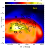
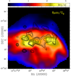
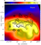
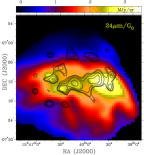
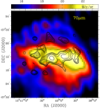
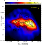
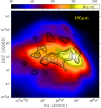
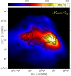
Figure 8: NIR maps of LDN 1780. The original maps are on the left and those corrected by the radiation field $G_{0}$ are on the right. From top to bottom, the first row is 8$\,\mu\mathrm{m}$, the second 24$\,\mu\mathrm{m}$, the third 70$\,\mu\mathrm{m}$ and the fourth 160$\,\mu\mathrm{m}$. The contours of the 31 GHz CARMA map are overlaid on all the maps. The $G_{0}$-corrected 8$\,\mu\mathrm{m}$ and 24$\,\mu\mathrm{m}$ maps (top two) show a better correlation with the 31 GHz data than the original 8$\,\mu\mathrm{m}$ and 24$\,\mu\mathrm{m}$ maps. The opposite occurs for the 70$\,\mu\mathrm{m}$ and 160$\,\mu\mathrm{m}$ (bottom two). In this case, the correction for the ISRF results in a worse correlation with the 31 GHz map compared to the original. The quantitative values of the correlation are listed in Table 7.

Table 7: Spearman’s rank, $r_{s}$, between the 31 GHz map and the different IR templates. The column on the centre shows the correlation value for the IR maps after they have been divided by the radiation field map, in order to account for variations in the illumination of the grains across the cloud. The column on the right shows the ratio between both quantities.

Wavelength	$r_{s}$	$r_{s}[G_{0}]$	$r_{s}[G_{0}]/r_{s}$
$[\micron]$
$8$	$0.14\pm 0.06$	$0.38\pm 0.07$	$2.7\pm 0.5$
$24$	$0.21\pm 0.06$	$0.46\pm 0.06$	$2.2\pm 0.3$
$70$	$0.49\pm 0.07$	$0.45\pm 0.07$	$0.9\pm 0.2$
$160$	$0.36\pm 0.07$	$0.31\pm 0.07$	$0.9\pm 0.3$
$250$	$0.35\pm 0.06$	$0.31\pm 0.07$	$0.9\pm 0.3$
$350$	$0.34\pm 0.06$	$0.30\pm 0.07$	$0.9\pm 0.3$
$500$	$0.34\pm 0.06$	$0.30\pm 0.06$	$0.9\pm 0.3$

We compare the emissivity at the peak of the 31 GHz map, with the emissivity of the region with largest column density of the cloud. In Fig. 9 we show these two regions and in Table 8 we list average values over a 2^′ diameter aperture for the column density, dust temperature, and the relative intensity of the ISRF obtained from the maps produced in Sec. 4. We also list the flux densities at 31 GHz in the 2^′ aperture and the ratio of the flux with the mean hydrogen column density.

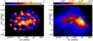
Figure 9: Left: 31 GHz CARMA map of LDN 1780. Right: hydrogen column density map obtained from the IR data in Section 4. Region 1 corresponds to the peak of the CARMA map while region 2 in centred at the peak of the column density map on the right. Both circular regions have 2^′ diameter.

Table 8: Parameters of the regions shown in Fig. 9. The column density, dust temperature and radiation field intensity $G_{0}$ are obtained from the map produced in Sec. 4. The fluxes at 31 GHz are integrated over a 2^′ diameter aperture. Their location is shown in Fig. 9.

Region	$N(H)$	$T_{d}$	$G_{0}$	$S_{31}$	$S_{31}/N(H)$
	[$\times 10^{21}$ cm-2]	[K]		mJy	$\times 10^{-24}$ [Jy cm-2]
1	2.4	16.6	0.7	4.5	18.7
2	7.3	15.0	0.4	2.4	3.2

Region 1 shows a 31 GHz emissivity which is $18.7/3.2=5.8$ times larger than that of Region No. 2. We will see if the SPDUST package from Ali-Haïmoud, Hirata & Dickinson (2009); Silsbee, Ali-Haïmoud & Hirata (2011) can produce emissivities different by a factor $\sim 5.8$ within this cloud, with plausible physical conditions.

In SPDUST, there are seven input parameters that are related to the environmental conditions of the emitting region. These are,

1. Total hydrogen number density $n_{H}$.

2. Gas temperature $T$.

3. Intensity of the radiation field relative to the average interstellar radiation field $G_{0}$.

4. Hydrogen ionization fraction $x_{H}\equiv n_{H^{+}}/n_{H}$.

5. Ionized carbon fractional abundance $x_{C}\equiv n_{C}+/n_{H}$.

6. Molecular hydrogen fractional abundance $y\equiv 2n(H_{2})/n_{H}$.

7. “line” parameter: Parameters that define the grain size distribution. It corresponds to the number line number of Table 1 of Weingartner & Draine (2001).

Another critical parameter is the shape of the grain size distribution. In LDN 1780, the differences in the IR morphology of the cloud can be explained by a difference in the type of grains across the cloud. Weingartner & Draine (2001) describe parametrizations of the grain size distribution, where the main dust components, silicates and carbonaceous grains are described. The grain size distribution of silicate grains has a power-law shape for the smallest grains, which are probably the ones responsible for some of the spinning dust emission. Carbonaceous grains on the other hand, show a more complicated distribution, with two “bumps” in the small-size regime. These local peaks are the small PAHs, large molecules with less than $\sim 10^{3}$ atoms. A larger abundance of C also increases the proportion of PAHs. PAHs are also expected to be important spinning dust emitters.

The number of PAHs in the SPDUST model, which is characterised by the relative size of the bumps in the grains size distribution, produces large differences in the emissivity at radio frequencies. We have modified the SPDUST package to allow modifications of the b_c parameter, which defines the relative size of the PAH bumps in the grain size distribution, for a fixed total carbon abundance. A similar analysis has recently been done by Tibbs et al. (2016).

The SPDUST code has been used by many authors to compare the AME emissivity with radio data. Normally, most parameters are kept fixed to standard values for different astrophysical environments (e.g. cold neutral medium, warm ionised medium). Here we would like to constrain the range of some parameters using additional datasets of LDN 1780. Different combinations of the SPDUST parameters can produce similar output spectra. Also, some of these parameters are strongly correlated. To tackle these complications, we use an exhaustive approach where we run SPDUST over a grid of parameters, for a total of 10⁷ runs. Table 9 lists the range and the spacing for each parameter.

Table 9: Range of the parameters used for defining the grid for running SPDUST. The parameters are: the hydrogen column density, gas temperature, intensity of the radiation field, hydrogen, carbon and H₂ fractional abundances. $b_{c}$ quantifies the proportion of PAH grains in the dust.

Parameter	min	max	Steps	Type
$n_{H}$	0.1	$10^{5}$	10	log
$T$	10	$10^{5}$	10	log
$\chi$	$10^{-4}$	3000	10	asinh
$x_{\rm H}$	$10^{-4}$	1	10	asinh
$x_{\rm C}$	$10^{-4}$	1	10	asinh
$y$	$10^{-4}$	1	10	asinh
$b_{\rm c}$	0	1	10	linear

From each run of SPDUST we recover the peak frequency, the peak emissivity and also the parameters that define a fourth order polynomial fit to the SPDUST spectrum. The polynomial fit is calculated around the peak of the spectrum. In order to explore the results from the SPDUST runs, we first use observational constraints from ancillary sources in some of the physical parameters in LDN 1780.

Mattila & Sandell (1979) observing neutral hydrogen and OH with the 100-m Effelsberg radio telescope found that the kinetic temperature of hydrogen was in the range $T_{k}=40-56$ K. They also quote a mean value for the total density of the gas of $n=1.8x10^{3}$ cm^-3​​. Laureijs et al. (1995) finds an average total density of 10³ cm^-3, while Toth et al. (1995) obtains a lower value of $0.6\times 10^{3}$ cm^-3. These two works also show that the cloud is in virial equilibrium and presents an $r^{-2}$ density profile.

We can assume that Region No. 1, which corresponds to the peak of the 31 GHz map, has a density equal to the average density of the cloud of 1000 cm^-3​​. This is reasonable as the column density at that point has a near-average value over the cloud (see left panel of Fig. 9). As this point is about half-way to the border of the cloud, and we know that the density profile of the cloud presents an $r^{-2}$ dependency, we can estimate the value of the highest density of the cloud to be $0.5^{-2}=4$ times larger than the average. We can also assume that the coldest region of the cloud will be the one with higher column density (this region also has the lowest dust temperature, as we shown in Section 4). We therefore assign to Region No. 2, the lowest gas temperature allowed by the work of Mattila & Sandell (1979), $T=40$ K. The largest temperature that Mattila & Sandell (1979) predicts for the cloud, $T=56$ K is assigned to Region 1. For the radiation field, we use the values that we calculated previously. Region 2, at the peak of the column density, is also coincident with a peak in the ¹³CO map from Toth et al. (1995), this implies that the ionization fraction in this region is very close to zero, due to the molecular nature of the gas at this position. For the ionization fraction, we use the value that Draine & Lazarian (1998) defines for the cold neutral medium (CNM), as listed in Table 10. The carbon ionization fractions for the two regions are also taken from the conditions for MC and CNM in Draine & Lazarian (1998). We list the parameters for Regions 1 and 2 in Table 10. We note that the absolute value of these parameters is not as important as the ratio between them, as we want to compare the ratio of the emissivities produced by SPDUST.

Table 10: SPDUST parameters of the regions shown in Fig. 9. The column density, dust temperature and radiation field intensity $G_{0}$ are obtained from the maps produced in Section 4. “line” corresponds to the parameters that define the grain size distribution, defined in Table 1 of Weingartner & Draine (2001), the parameters listed in line 7 are the favored by Weingartner & Draine (2001) for the Milky Way. The locations of Reg 1 and Reg 2 are shown in Fig. 9.

Region	$n(H)$	$T$	$G_{0}$	$x_{H}$	$x_{C}$	$y$	“line”
	cm-3	[K]					WD2001
MC	300	20	0.01	0	0.0001	0.99	7
CNM	30	100	1	0.0012	0.0003	0	7
Reg 1	1000	56	0.7	0.0012	0.0003	0.5	7
Reg 2	4000	40	0.4	0	0.0001	0.99	7

In Fig. 10 we show the resulting spectra for regions 1 and 2, using the parameters listed in Table 10. The difference in the parameters produces a difference in emissivity that is almost zero at 31 GHz and only 21% at the peak of each spectrum, around 75 GHz. This is not unexpected due to the small variation in the parameters from region 1 to region 2. This shows that variation in the environmental conditions are not sufficient to explain the emissivity differences observed in the cloud.

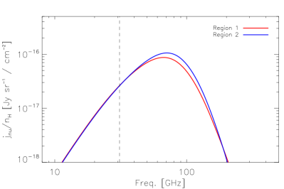
Figure 10: SPDUST spectra for regions 1 and 2, using the parameters listed in Table 10. The vertical dashed line in all the plots marks the frequency of our CARMA data, 31 GHz.

The number of PAHs in the SPDUST model, which is characterised by the relative size of the bumps in the grain size distribution, produces large differences in the emissivity at radio frequencies. If we allow this value to change across the cloud, we can reproduce the observed differences in radio emissivity. In Fig. 11 we show the SPDUST spectra for Region 1 and 2 using the same parameters of Table 10, but this time changing the “line” parameter to represent a variation in carbon abundance by a factor 6. By doing this, the emissivity ratio at 31 GHz is 5.5, close to the measured 5.8 from the CARMA data.

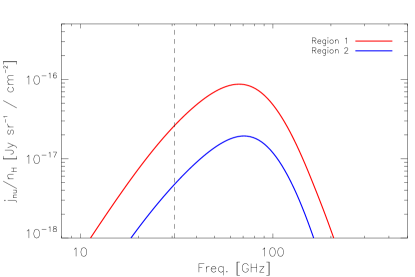
Figure 11: SPDUST spectra for regions 1 and 2, using the parameters listed in Table 10, but this time, changing the “line” parameter, to change the grain size distribution by increasing the total carbon abundance. In this case, the ratio of the two spectra at 31 GHz (showed with the dashed line) is 5.5, close to the measured 5.8 from the CARMA data.

A factor of six in the total carbon abundance is difficult to explain given the proximity of the two regions in the same cloud. An alternative to such a drastic change in the chemical composition of the cloud is to modify the relative size of the PAH bumps in the grain size distribution, for a fixed total carbon abundance. The values quoted by Weingartner & Draine (2001), of 0.75 and 0.25 for the amplitude of the large and small peaks represent a best-fit value to a number of different clouds, so they will likely differ from cloud to cloud.

It is clear that, given the degrees of freedom of SPDUST, the observed differences in emissivity across the cloud are compatible with spinning dust. Nevertheless, we have shown that if we constrain the parameter space to be compatible with the physical properties of the cloud found in the literature, the variations in 31 GHz emissivity observed in the CARMA data cannot be explained only by environmental variations. We explored the parameter space within the values listed in Table 10 that are compatible with the observed emissivity for Regions 1 and 2 listed in Table 8. We find that the only models compatible with the observed emissivities present a different grain size distribution ($b_{\rm c}$ parameter). In is important to note that Ridderstad et al. (2006) reached the same conclusion, in requiring a significant variation in the grain size distribution along the E-W axis of LDN 1780, but based on the study of infrared data and radiative transfer modelling.

These differences in the grain properties across the cloud can be expected, as there are differences in the IR morphology of the cloud. In this scenario, the denser region of the cloud, which shows low radio emission has a smaller proportion of the smallest PAHs, and this fraction is $\sim 9$ times larger at the peak of the 31 GHz emission. The origin for this difference might be related to the coagulation of the smallest grains in the denser and colder region of LDN 1780.

5 Conclusions

Following the detection of AME in the LDN 1780 translucent cloud presented in Vidal et al. (2011) using data from the Cosmic Background Imager (CBI), we performed follow-up observations at 31 GHz using the CARMA 3.5-m array. These new data have an angular resolution of $2^{\prime}$, 3 times better than that of the CBI. We measured the correlation between the 31 GHz data and different IR templates. We found that the best correlation occurs with MIPS $70\,{\mu}$m, with a Spearman’s rank $r_{S}=0.49\pm 0.07$. This confirms what we found using the CBI data in Vidal et al. (2011), where the radio data correlated better with a 60 $\mu$m IR map. The correlation between the CARMA data and Spitzer $8\micron$ and Spitzer 24 $\mu$m, which traces PAHs and VSGs, is poor. Here, $r_{S}=0.14\pm 0.06$ and $r_{S}=0.21\pm 0.06$ for 8 $\mu$m and 24 $\mu$m respectively. These two correlation values increase significantly when correcting the IR maps by the ISRF, yielding $r_{S}=0.38\pm 0.07$ and $r_{S}=0.46\pm 0.06$ for the corrected 8 $\mu$m and 24 $\mu$m templates respectively. This is important as these ISRF corrected templates should be better tracers of the PAHs and VSGs column density, as opposed to the uncorrected maps, in which the emission is proportional also to the incoming radiation field.

We constructed an SED of LDN 1780 on 1^∘ scales between 0.408 GHz and 2997 GHz, including Planck data. The region of the cloud is dominated by the CMB anisotropy between 23 GHz and 217 GHz. After subtraction of the CMB emission, the presence of AME is very clear and it is well fitted using a spinning dust model. AME is detected with a significance $>20\sigma$. On these angular scales, there is a significant shift of the peak of the cloud between the emission at low frequencies (23–70 GHz) versus the emission at higher frequencies (93–2997 GHz). This means that the AME in this cloud does not originate at the same location that the thermal dust emission.

In the 31 GHz CARMA maps, there are differences in the emissivity along the cloud. These differences are compatible with the spinning dust model. The spinning dust emission depends on the physical parameters of the dust grain and also on environmental conditions of the cloud, such as density, temperature and ISRF. Some of these parameters for LDN 1780 are known from the literature, so we fixed them and concluded that there must be variations in the grain size distribution along the cloud, with and E–W enhancement of the PAHs population. Only by doing this the model can reproduce the observed factor $\sim 6$ difference in the AME emissivity.

Given the large number of free parameters that the spinning dust models have, it is not difficult to account for AME variations in different environments. This is something to keep in mind when trying to interpret the observations. It is clear that a greater number of observations are required in order to fully constrain the spinning dust models. Multi-wavelength observations are needed in order to constrain parameters independently. In particular, separating different grain populations. High angular resolution observations of AME sources using current and future instruments (VLA, ALMA, ngVLA, SKA) will help greatly in this respect.

References

- Ali-Haïmoud, Hirata & Dickinson (2009) Ali-Haïmoud Y., Hirata C. M., Dickinson C., 2009, MNRAS, 395, 1055
- AMI Consortium et al. (2009) AMI Consortium et al., 2009, MNRAS, 400, 1394
- Battistelli et al. (2015) Battistelli E. S. et al., 2015, ApJ, 801, 111
- Bennett et al. (2013) Bennett C. L. et al., 2013, ApJS, 208, 20
- Bertin & Arnouts (1996) Bertin E., Arnouts S., 1996, A&AS, 117, 393
- Casassus et al. (2006) Casassus S., Cabrera G. F., Förster F., Pearson T. J., Readhead A. C. S., Dickinson C., 2006, ApJ, 639, 951
- Casassus et al. (2008) Casassus S. et al., 2008, MNRAS, 391, 1075
- Castellanos et al. (2011) Castellanos P. et al., 2011, MNRAS, 411, 1137
- Condon et al. (1998) Condon J. J., Cotton W. D., Greisen E. W., Yin Q. F., Perley R. A., Taylor G. B., Broderick J. J., 1998, AJ, 115, 1693
- Cornwell & Evans (1985) Cornwell T. J., Evans K. F., 1985, A&A, 143, 77
- Dickinson et al. (2018) Dickinson C. et al., 2018, New Astronomy Reviews, 80, 1
- Dickinson et al. (2010) Dickinson C. et al., 2010, MNRAS, 407, 2223
- Dickinson et al. (2009) Dickinson C. et al., 2009, ApJ, 690, 1585
- Dickinson et al. (2007) Dickinson C., Davies R. D., Bronfman L., Casassus S., Davis R. J., Pearson T. J., Readhead A. C. S., Wilkinson P. N., 2007, MNRAS, 379, 297
- Draine (2011) Draine B. T., 2011, Physics of the Interstellar and Intergalactic Medium. Princeton University Press
- Draine & Lazarian (1998) Draine B. T., Lazarian A., 1998, ApJ, 508, 157
- Erickson (1957) Erickson W. C., 1957, ApJ, 126, 480
- Finkbeiner et al. (2002) Finkbeiner D. P., Schlegel D. J., Frank C., Heiles C., 2002, ApJ, 566, 898
- Fixsen (2009) Fixsen D. J., 2009, ApJ, 707, 916
- Franco (1989) Franco G. A. P., 1989, A&A, 223, 313
- Gaustad et al. (2001) Gaustad J. E., McCullough P. R., Rosing W., Van Buren D., 2001, PASP, 113, 1326
- Górski et al. (2005) Górski K. M., Hivon E., Banday A. J., Wandelt B. D., Hansen F. K., Reinecke M., Bartelmann M., 2005, ApJ, 622, 759
- Greaves et al. (2018) Greaves J. S., Scaife A. M. M., Frayer D. T., Green D. A., Mason B. S., Smith A. M. S., 2018, Nature Astronomy
- Haslam et al. (1982) Haslam C. G. T., Salter C. J., Stoffel H., Wilson W. E., 1982, A&AS, 47, 1
- Hauser et al. (1998) Hauser M. G. et al., 1998, ApJ, 508, 25
- Hensley, Draine & Meisner (2016) Hensley B. S., Draine B. T., Meisner A. M., 2016, ApJ, 827, 45
- Hoang, Draine & Lazarian (2010) Hoang T., Draine B. T., Lazarian A., 2010, ApJ, 715, 1462
- Hoang & Lazarian (2012) Hoang T., Lazarian A., 2012, ApJ, 761, 96
- Hoang et al. (2018) Hoang T., Nguyen-Quynh L., Nguyen-Anh V., Kim Y.-J., 2018, ArXiv e-prints
- Högbom (1974) Högbom J. A., 1974, A&AS, 15, 417
- Jonas, Baart & Nicolson (1998) Jonas J. L., Baart E. E., Nicolson G. D., 1998, MNRAS, 297, 977
- Laureijs et al. (1995) Laureijs R. J., Fukui Y., Helou G., Mizuno A., Imaoka K., Clark F. O., 1995, ApJS, 101, 87
- Leitch et al. (1997) Leitch E. M., Readhead A. C. S., Pearson T. J., Myers S. T., 1997, ApJ, 486, L23+
- Markwardt (2009) Markwardt C. B., 2009, in Astronomical Society of the Pacific Conference Series, Vol. 411, Astronomical Data Analysis Software and Systems XVIII, Bohlender D. A., Durand D., Dowler P., eds., p. 251
- Mathis, Mezger & Panagia (1983) Mathis J. S., Mezger P. G., Panagia N., 1983, A&A, 128, 212
- Mattila & Sandell (1979) Mattila K., Sandell G., 1979, A&A, 78, 264
- Murphy et al. (2010) Murphy E. J. et al., 2010, ApJ, 709, L108
- Murphy et al. (2018) Murphy E. J., Linden S. T., Dong D., Hensley B. S., Momjian E., Helou G., Evans A. S., 2018, ApJ, 862, 20
- Planck Collaboration et al. (2014a) Planck Collaboration et al., 2014a, A&A, 571, A11
- Planck Collaboration et al. (2011a) Planck Collaboration et al., 2011a, A&A, 536, A25
- Planck Collaboration et al. (2016a) Planck Collaboration et al., 2016a, A&A, 594, A1
- Planck Collaboration et al. (2016b) Planck Collaboration et al., 2016b, A&A, 594, A10
- Planck Collaboration et al. (2016c) Planck Collaboration et al., 2016c, A&A, 594, A9
- Planck Collaboration et al. (2014b) Planck Collaboration et al., 2014b, A&A, 571, A13
- Planck Collaboration et al. (2016d) Planck Collaboration et al., 2016d, A&A, 594, A25
- Planck Collaboration et al. (2014c) Planck Collaboration et al., 2014c, A&A, 565, A103
- Planck Collaboration et al. (2011b) Planck Collaboration et al., 2011b, A&A, 536, A1
- Planck Collaboration et al. (2011c) Planck Collaboration et al., 2011c, A&A, 536, A20
- Reich & Reich (1986) Reich P., Reich W., 1986, A&AS, 63, 205
- Reich, Testori & Reich (2001) Reich P., Testori J. C., Reich W., 2001, A&A, 376, 861
- Reich (1982) Reich W., 1982, A&AS, 48, 219
- Remazeilles et al. (2015) Remazeilles M., Dickinson C., Banday A. J., Bigot-Sazy M.-A., Ghosh T., 2015, MNRAS, 451, 4311
- Ridderstad et al. (2006) Ridderstad M., Juvela M., Lehtinen K., Lemke D., Liljeström T., 2006, A&A, 451, 961
- Sault, Teuben & Wright (1995) Sault R. J., Teuben P. J., Wright M. C. H., 1995, in Astronomical Society of the Pacific Conference Series, Vol. 77, Astronomical Data Analysis Software and Systems IV, Shaw R. A., Payne H. E., Hayes J. J. E., eds., p. 433
- Scaife et al. (2010) Scaife A. M. M. et al., 2010, MNRAS, 403, L46
- Silsbee, Ali-Haïmoud & Hirata (2011) Silsbee K., Ali-Haïmoud Y., Hirata C. M., 2011, MNRAS, 411, 2750
- Snow & McCall (2006) Snow T. P., McCall B. J., 2006, ARA&A, 44, 367
- Tibbs et al. (2011) Tibbs C. T. et al., 2011, MNRAS, 418, 1889
- Tibbs et al. (2016) Tibbs C. T. et al., 2016, MNRAS, 456, 2290
- Todorović et al. (2010) Todorović M. et al., 2010, MNRAS, 406, 1629
- Toth et al. (1995) Toth L. V., Haikala L. K., Liljestroem T., Mattila K., 1995, A&A, 295, 755
- Vidal et al. (2011) Vidal M. et al., 2011, MNRAS, 414, 2424
- Watson et al. (2005) Watson R. A., Rebolo R., Rubiño-Martín J. A., Hildebrandt S., Gutiérrez C. M., Fernández-Cerezo S., Hoyland R. J., Battistelli E. S., 2005, ApJ, 624, L89
- Weingartner & Draine (2001) Weingartner J. C., Draine B. T., 2001, ApJ, 548, 296
- Witt et al. (2010) Witt A. N., Gold B., Barnes, III F. S., DeRoo C. T., Vijh U. P., Madsen G. J., 2010, ApJ, 724, 1551
- Ysard, Juvela & Verstraete (2011) Ysard N., Juvela M., Verstraete L., 2011, A&A, 535, A89
- Ysard, Miville-Deschênes & Verstraete (2010) Ysard N., Miville-Deschênes M. A., Verstraete L., 2010, A&A, 509, L1