A Volterra-series approach to stochastic nonlinear dynamics: The Duffing oscillator driven by white noise

Abstract

The Duffing oscillator is a paradigm of bistable oscillatory motion in physics, engineering, and biology. Time series of such oscillations are often observed experimentally in a nonlinear system excited by a spontaneously fluctuating force. One is then interested in estimating effective parameter values of the stochastic Duffing model from these observations—a task that has not yielded to simple means of analysis. To this end we derive theoretical formulas for the statistics of the Duffing oscillator’s time series. Expanding on our analytical results, we introduce methods of statistical inference for the parameter values of the stochastic Duffing model. By applying our method to time series from stochastic simulations, we accurately reconstruct the underlying Duffing oscillator. This approach is quite straightforward—similar techniques are used with linear Langevin models—and can be applied to time series of bistable oscillations that are frequently observed in experiments.

Some of the most interesting and complex behaviors in nature emerge from coupled systems with nonlinearities embedded in an environment. Depending on the relevant time and length scales, influences from the environment can be described effectively as fluctuating forces driving such systems. A fundamental example of such a system is the stochastic Duffing oscillator, which, together with its generalizations, has various applications in engineering and biophysics Khan and Vyas (2001); Chatterjee and Vyas (2003); Alonso et al. (2014); Mindlin (2017); Cherevko et al. (2016); Parshin et al. (2016); Cherevko et al. (2017); Izhikevich and FitzHugh (2006). The Duffing equation offers the simplest nonlinear model that describes bistable oscillatory motion (Strogatz, 2014, Sec. 7.6). Under certain physical conditions the equation represents a power-series approximation for a general class of Lienard systems (Strogatz, 2014, Sec. 7.4).

The Duffing model extends the harmonic oscillator by adding a cubic nonlinear term:

$$\ddot{x}+a\dot{x}+bx+cx^{3}=f$$ (1)

for an unknown function of time $x(t)$ and an external force $f(t)$. The constants $a$, $b$, and $c$ are the damping coefficient, the linear stiffness, and the cubic Duffing parameter, respectively. Because the above equation is of second order in time, the phase of this system is specified by two degrees of freedom $(x,\dot{x})$.

In various situations the form of the relevant driving force is $f(t)=A\dot{w}(t)$, in which $A>0$ is a constant and $\dot{w}(t)$ is Gaussian white noise of zero mean and unit intensity. Equation (1) describes a stable dynamical system when the coefficients $a>0$ and $c>0$ are strictly positive. Unlike the harmonic oscillator, for which $c=0$, the Duffing model admits a negative linear stiffness $b$.

The Duffing oscillator is bistable when $b<0$. Its phase space is symmetric about the origin $(x,\dot{x})=(0,0)$, which represents an unstable fixed point in absence of external force. Two stable equilibria occur at $(\xi,0)$ and $(-\xi,0)$, in which $x=\pm\xi=\pm\sqrt{-b/c}$ correspond to the minima of the Duffing double-well potential $U(x)=\operatorname{\mathrm{const}}+bx^{2}/2+cx^{4}/4$. In the monostable regime, for which $b\geq 0$, the origin is the only fixed point.

A problem that arises often in quantitative studies of bistable nonlinear systems is the determination of a model’s parameter values. In experiments one usually observes time series of noisy oscillations. The model parameters may then be adjusted empirically to reproduce the measurements as closely as possible. This method is rather arbitrary and imprecise, whereas other available approaches require additional experimental data Chatterjee (2010); Chatterjee and Vyas (2003); Smelyanskiy et al. (2005); He et al. (2007); Quaranta et al. (2010).

Although a time series of oscillations may in principle contain enough information to infer the parameter values of the Duffing oscillator, this approach has not been duly pursued. In the present letter we derive statistical formulas for the time series $x(t)$ in the regime of bistable oscillations. These expressions rely on the Volterra expansion of functionals (Rugh, 1981, Chapters 1-3), which provide the mathematical framework of nonlinear response theory Peterson (1967). Expanding on our analytical results, we then develop statistical methods to estimate the parameter values of the stochastic Duffing Eq. (1) from the time series $x(t)$.

General theory.—The functional series of Volterra generalize the Taylor-Maclaurin expansion of functions in calculus (Rugh, 1981, Sec. 1.5). In particular, we can represent the solution of Eq. (1) as a functional of the force $f(t)$:

$$x(t|f)=x_{0}(t)+\int_{0}^{t}dt_{1}\,g_{1}(t-t_{1})f(t_{1})\\ +\iint_{0}^{t}dt_{1}dt_{2}\,g_{2}(t-t_{1},t-t_{2})f(t_{1})f(t_{2})+...\\ =x_{0}(t)+\gamma_{1}(t)+\gamma_{2}(t)+...$$ (2)

Here $g_{1}$ and $g_{2}$ are the Volterra kernels of the linear and quadratic terms in $f$, $\gamma_{1}(t)$ and $\gamma_{2}(t)$, respectively.

Provided that the series (2) converge, a truncated Volterra expansion approximates the solutions of Eq. (1). We find the unknown kernels $g_{i=1,2...}$ by using the variational approach (Rugh, 1981, Sec. 3.4): we replace the external force $f(t)$ by a constant $f_{c}\equiv\operatorname{\mathrm{const}}$ and substitute Eq. (2) into (1). Then, by collecting terms with coefficients of equal powers in $f_{c}$, we obtain the following system of equations

$$0 = \ddot{x}_{0}+a\dot{x}_{0}+bx_{0}+cx_{0}^{3},$$ (3)

$$f = \ddot{\gamma}_{1}+a\dot{\gamma}_{1}+b\gamma_{1}+3cx_{0}^{2}\gamma_{1},$$ (4)

$$0 = \ddot{\gamma}_{2}+a\dot{\gamma}_{2}+b\gamma_{2}+3c(x_{0}\gamma_{1}^{2}+x_{0}^{2}\gamma_{2}),$$

$$...$$

Equation (3), which defines $x_{0}(t)$, is equivalent to the homogeneous Duffing problem (1) with $f\equiv 0$. The Volterra kernels can be found in successively increasing orders from the linear Eqs. (4), ( A Volterra-series approach to stochastic nonlinear dynamics: The Duffing oscillator driven by white noise), etc.

The equilibrium solution $x_{0}(t)\equiv 0$ of Eq. (3) spawns a particularly convenient set of Eqs. (4) and ( A Volterra-series approach to stochastic nonlinear dynamics: The Duffing oscillator driven by white noise) for the monostable Duffing oscillator Khan and Vyas (2001). In the bistable case, the kernels of the Volterra series at $x_{0}(t)\equiv 0$ diverge with $t\to\infty$ (Note, , Secs. I and II). In fact, this expansion may even fail to exist Ku and Wolf (1966). Therefore we develop the Volterra series at the stable equilibria $x_{0}(t)\equiv\pm\xi$.

As a generalization of the Taylor-Maclaurin series, the Volterra expansion may be limited by a convergence region. Moreover the accuracy of the truncated expression deteriorates as $f(t)$ becomes progressively greater: the relevant physical scales are introduced later. Due to the symmetry of the Duffing oscillator, $x_{0}(t)\equiv\xi$ and $x_{0}(t)\equiv-\xi$ lead to identical odd-order terms in Eq. (2), whereas the even-order terms differ by a factor of $-1$ (Note, , Sec. II). As we show shortly, these two series are accurate in the neighborhood of the expansion points as long as the system’s trajectory $x(t)$ does not cross the special point $x=0$.

If the amplitude $A$ of the external force $f(t)$ is small, the Duffing oscillator remains in one of the two potential wells at $x=\pm\xi$. The truncated Volterra expansions then describe the solutions of Eq. (1) accurately around the respective equilibrium points. The linear response of $x(t)$ is harmonic in the first order of the parameter $A$,

$$\ddot{\gamma}_{1}+a\gamma_{1}-2b\gamma_{1}=f,$$ (6)

which can also be obtained by linearization of Eq. (1) at the minima of the Duffing potential.

When $A$ is sufficiently large, the Duffing oscillator undergoes stochastic transitions between the two potential wells. The statistical average $\langle x\rangle=0$ vanishes due to the symmetry of the problem. Although truncated Volterra expansions of $x(t)$ are inaccurate in this case, Eq. (2) may still be applied to describe pieces of the oscillator’s trajectory in an $\varepsilon$-neighborhood of each potential well ($|x(t)\pm\xi|\leq\varepsilon<\xi$). A physical assumption is implied thereby that the external force does not perturb the system’s energy much while the oscillator remains in one of the wells. In this sense the argument $f$ of the functional Eq. (2) is small. Statistically the selected pieces of the oscillator’s trajectory belong to two ensembles of conditional probability distributions $p(x_{\xi})=p(x|\,|x-\xi|\leq\varepsilon)$ and $p(x_{-\xi})=p(x|\,|x+\xi|\leq\varepsilon)$ [Asimilarapproachhasalreadybeenappliedin][; Sec.4todescribefluctuationsinametastabledynamicalsystem.]Belousov2014.

The energy barrier that separates the two wells of the Duffing potential becomes negligible for external forces of extreme amplitudes $A$. The oscillations then resemble those of a monostable regime.

Statistical analysis.—The time-invariant probability density of a bistable Duffing oscillator driven by white noise is generally bimodal. Two Gaussian-like peaks correspond to the minima of the double-well potential $U(x)$, for which the harmonic oscillator Eq. (6) describes the local dynamics of $x(t)$. We can construct the time-invariant probability density of $x$ by using an exponential form:

$$p(x)\approx Z^{-1}\exp[-P(x)+\mathcal{O}(x^{5})],$$ (7)

in which $Z$ is a normalization constant and $P(x)\geq 0$ is a polynomial of fourth order in $x$ Belousov et al. (2016, 2014). At the two global minima of Eq. (7) the following conditions must be satisfied:

$$P(\pm\xi)=0,\quad\frac{\partial^{2}P}{\partial x^{2}}(\pm\xi)=-4ab/A^{2}.$$

The last equality ensures that the Laplace approximation of $p(x)$ at $x=\pm\xi$ Touchette (2009) obeys the statistics of Eq. (6) (Chandrasekhar, 1943, Sec. II-3). Owing to the symmetry of the bistable Duffing system $p(x)=p(-x)$, the general form of $P(x)$ is given by

$$P(x)=\frac{ac(x^{2}-\xi^{2})^{2}}{2A^{2}},$$

which leads to

$$p(x)\approx Z^{-1}\exp\left[-\frac{ac(x^{2}-\xi^{2})^{2}}{2A^{2}}\right]\propto\exp\left[-\frac{2aU(x)}{A^{2}}\right].$$ (8)

The normalization constant $Z$ can be found by integration of the exponential factor in the above equation:

$$Z=\frac{\pi\xi}{2}\exp(-z)[I_{-1/4}(z)+I_{1/4}(z)],$$

in which $z=ac\xi^{4}/(4A^{2})$ and $I_{i}(\cdot)$ is the $i$^th-order modified Bessel function of the first kind.

In addition the autocorrelation function $\chi(t)$ can be approximately calculated for $x_{\pm\xi}(t)$ from Eq. (6) Belousov and Cohen (2016):

$$\chi(t)\approx\chi_{1}(t)=\frac{\langle\gamma_{1}(0)\gamma_{1}(t)\rangle}{\langle\gamma_{1}\rangle^{2}}\\ =\exp\left(-\frac{a\,|t|}{2}\right)\left[\cos(\Omega\,|t|)+\frac{a}{2\Omega}\sin(\Omega\,|t|)\right],$$ (9)

in which $\Omega=\sqrt{-2b-a^{2}/4}$ .

Dimensional analysis.—Equations (1), (8), and (9) characterize physical scales of the Duffing oscillator. First we adopt the constants $a^{-1}$ and $a/\sqrt{c}$ as the units of $t$ and $x$ respectively. The energy scales are then determined by the height of the barrier between the wells of the Duffing potential $\epsilon=b^{2}/(4c)$. It suffices therefore to consider $b=-2\sqrt{\epsilon c}$ as a typical value for a unit energy barrier $\epsilon$.

The Boltzmann-like factor $\exp[-2aU(x)/A^{2}]$ in Eq. (8) relates the level of energy fluctuations $A^{2}/(2a)$ in the system to the Duffing potential $U(x)$. This helps us identify the amplitudes of the external force $A\lesssim\sqrt{2a\epsilon}$, for which the truncated Volterra series might be useful to describe the trajectories $x_{\pm\xi}(t)$.

Because Eq. (9) was derived from the linear-response approximation, it is independent of $A$. Although this formula is very convenient, its accuracy is limited to small time and energy scales, as shown below. The autocorrelation function Eq. (9) decays exponentially with a relaxation time $\tau\approx a^{-1}$ Zwanzig and Ailawadi (1969). In general we may expect the formula (9) to hold for $0\leq t\lesssim\tau$.

Parametric inference.—To test our theoretical results we simulated Eq. (1) (Note, , Sec. IV) by using an operator-splitting algorithm (Tuckerman et al., 1992; Belousov et al., 2017, Appendix C). The results are reported in the system of units reduced by the time, length, and energy constants $a^{-1}$, $a/\sqrt{c}$, and $\epsilon$, respectively. As justified earlier, the constant $b=-2$ is fixed. Our simulations differ only by values of the parameter $A$.

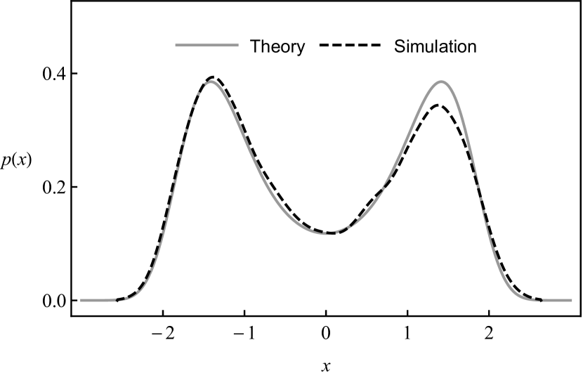
Figure 1: Steady-state probability density $p(x)$ for the time series simulated with $A=1.3$. The theoretical expression is given by Eq. (8), whereas the computational results are represented by a smooth histogram Mat (2018).

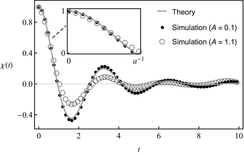
Figure 2: Time autocorrelation function $\chi(t)$ for time series $x(t)$ driven by a weak external force ($A=0.1$) and for the time series $x_{\varepsilon}(t)$ ($A=1.1$). Error bars, which are comparable in size to the plot markers, are omitted. The theoretical curve corresponds to Eq. (9). The inset magnifies the exponential decay for $t\lesssim a^{-1}$.

Table 1: Statistical inference of parameter values for the Duffing oscillator Eq. (1), which was simulated with fixed values $a=1$, $b=-2$, and $c=1$; $A$ varied in the range $[0.6,1.3]$. The estimated parameter values are denoted by $\hat{a}$, $\hat{b}$, $\hat{c}$, and $\hat{A}$, respectively. The uncertainties are given by three standard deviations calculated as described in (Note, , Sec. III).

$A$	$\hat{a}$	$\hat{b}$	$\hat{c}$	$\hat{A}$
$0.6$	$1.06\pm 0.16$	$-2.03\pm 0.48$	$1.02\pm 0.24$	$0.63\pm 0.15$
$0.7$	$1.13\pm 0.14$	$-2.00\pm 0.43$	$1.01\pm 0.22$	$0.75\pm 0.13$
$0.8$	$1.17\pm 0.15$	$-2.09\pm 0.43$	$1.05\pm 0.22$	$0.91\pm 0.13$
$0.9$	$1.13\pm 0.18$	$-2.07\pm 0.46$	$1.04\pm 0.23$	$0.99\pm 0.15$
$1.0$	$1.14\pm 0.19$	$-2.16\pm 0.45$	$1.08\pm 0.22$	$1.12\pm 0.15$
$1.1$	$1.14\pm 0.21$	$-2.15\pm 0.39$	$1.08\pm 0.20$	$1.21\pm 0.14$
$1.2$	$1.15\pm 0.28$	$-2.27\pm 0.39$	$1.14\pm 0.20$	$1.37\pm 0.17$
$1.3$	$1.08\pm 0.42$	$-2.33\pm 0.34$	$1.16\pm 0.17$	$1.44\pm 0.23$

Histograms of the time series $x(t)$ agree with Eq. (8) for all values of the parameter $A$ that we explored (Fig. 1). When a simulation does not last long enough to observe sufficiently many transitions over the energy barrier $\epsilon$, the sample of $x$ may be biased toward the Duffing potential well in which the oscillator spends more time. The symmetry $p(-x)=p(x)$ may therefore appear imperfect in histograms of $x$. Another issue may emerge if the time resolution of the sample $x(t)$ is not sufficient to observe the trajectory of fast transitions between the two wells ($-\xi<x<\xi$). In this case the histogram’s peaks overestimate the probability density at $x\approx\pm\xi$ and underestimate it at $x\approx 0$ with respect to Eq. (8).

By using the maximum-likelihood fitting of Eq. (8) to the time series, we can determine the values of the parameters $\xi$ and $\sigma=A/\sqrt{ac}$. The density $p(x)$ estimated in this way is graphically indistinguishable from the theoretical prediction plotted in Fig. 1. Because Eq. (8) is not sensitive to the sample biases that are discussed above, the curve fitting of $p(x)$ yields very reliable results.

The trajectories $x_{\pm\xi}(t)$ were selected from the time series $x(t)$ with $\varepsilon=3\sigma/(2\xi)$ . Profiting from the symmetry of Eq. (1), we combined these two samples: $\{x_{\varepsilon}(t)\}=\{x_{\xi}(t)\}\cup\{|x_{-\xi}(t)|\}$. As expected, the local time autocorrelation function of $x_{\varepsilon}(t)$ agrees well with Eq. (9) in the interval $0\leq t\lesssim a^{-1}$ (Fig. 2). When the external force is too weak to drive transitions between the potential wells of the Duffing oscillator, the same theoretical expression matches perfectly the autocorrelation function of $x(t)$.

The local time autocorrelation function of $x_{\varepsilon}(t)$ has an undulatory shape. Note that Eq. (9) predicts quite accurately the frequency of these undulations even when $t\gg a^{-1}$; the discrepancy is due to their amplitude. This observation can be explained by considering higher-order contributions $\gamma_{i=2,3...}$ (Note, , Sec. III).

Good estimates of the frequency $\Omega$ can be obtained by fitting Eq. (9) to the time-series autocorrelations at small $t\lesssim a^{-1}$. The parameter $a$ that controls the decay of the amplitude of $\chi(t)$, however, is very sensitive to small errors introduced by the approximate expression $\chi_{1}(t)$. Because the second-order correction from Eq. (2) already leads to an unwieldy expression for $\chi(t)$, we propose instead a phenomenological equation motivated by the general form of higher-order Volterra kernels (Note, , Sec. III):

$$\chi(t)\approx\hat{\chi}(t)=(1-\alpha)\exp(-a\,|t|)\\ +\exp(-a\,|t|/2)[\alpha\cos(\Omega\,|t|)+\beta\sin(\Omega\,|t|)],$$ (10)

in which $\alpha$ and $\beta$ are unknown parameters, whereas the explicit expression can be substituted for $\Omega=\sqrt{-2b-a^{2}/4}$.

Curve fitting of Eq. (10) on the interval $0\leq t\lesssim a^{-1}$ with four unknown parameters—$a$, $b$, $\alpha$, and $\beta$—yields quite accurate values for $a$ and $b$. Technical details of this procedure are available in (Note, , Sec. III). The numerical values of $c$ and $A$ can be found from the estimates of $a$, $b$, $\xi$, and $\sigma$ (Table 1).

As shown above, the values of all four parameters of Eq. (1)—$a$, $b$, $c$, and $A$—can be inferred from the bistable time series $x(t)$. Our approach is limited to moderate noise intensities $A\sim\sqrt{a\epsilon}$, for which the first term of the Volterra expansion provides a tenable approximation (Table 1). In a sense this method extends the statistical techniques that were developed for the harmonic oscillator driven by white noise Belousov and Cohen (2016); Belousov et al. (2017).

A precise quantitative description of stochastic nonlinear systems is necessary to advance our understanding of complex behaviors observed in physics, engineering, and biology. The Volterra expansion offers important insights into the statistical theory of such systems. In a future communication we will present analysis of another classical model, the Van der Pol oscillator. The convergence issues of Eq. (2) may also stimulate interest in the Wiener theory of orthogonal functional series (Schetzen, 2006, Chapter 9). This development might even lead to more advanced theoretical results for the time autocorrelation function of a nonlinear oscillator. As we demonstrated above, the analysis of autocorrelations may provide a reliable estimation of a model’s parameter values from experimental measurements.

Supplemental Material

I The monostable Duffing oscillator

In this section we review the Volterra-series representation of solutions for the Duffing Eq. (1) in the monostable regime of oscillations ($b\geq 0$) Khan and Vyas (2001). Because we study a stationary problem endowed with a time-invariant probability density, Eq. (2) can be recast as

$$x(t|f)=x_{0}+\int_{-\infty}^{\infty}dt_{1}\,g_{1}(t-t_{1})f(t_{1})\\ +\iint_{-\infty}^{\infty}dt_{1}dt_{2}\,g_{2}(t-t_{1},t-t_{2})f(t_{1})f(t_{2})+...\\ =x_{0}(t)+\gamma_{1}(t)+\gamma_{2}(t)+...,$$ (11)

in which the integration limits are extended to infinities by invoking the causality of the kernels $g_{i}(...,t_{j},...)=0$ when $t_{j}\leq 0$, and by assuming the initial condition $x(-\infty)=x_{0}\equiv\operatorname{\mathrm{const}}$. We will omit indication of the infinite integration limits in the following.

The trivial equilibrium of Eq. (3) is the most convenient expansion point $x_{0}\equiv 0$ for Eq. (11). Equations (4), ( A Volterra-series approach to stochastic nonlinear dynamics: The Duffing oscillator driven by white noise), etc. then become

$$\ddot{\gamma}_{1}+a\dot{\gamma}_{1}+b\gamma_{1} = f,$$ (12)

$$\ddot{\gamma}_{2}+a\dot{\gamma}_{2}+b\gamma_{2} = 0,$$ (13)

$$\ddot{\gamma}_{3}+a\dot{\gamma}_{3}+b\gamma_{3} = -c\gamma_{1}^{3},$$

$$...$$

The above equations describe essentially the same harmonic oscillator

$$\ddot{\gamma}_{i}+a\dot{\gamma}_{i}+b\gamma_{i}=f_{i}$$ (15)

subject to different forcing terms $f_{i}=f,0,-c\gamma_{1}^{3}...$ The left-hand side of Eq. (15) corresponds to the linearized Duffing system that can be obtained by neglecting the nonlinear cubic term in Eq. (1).

By definition the Green function of Eq. (15) is the linear Volterra kernel $g_{1}$:

$$\gamma_{1}(t)= \int ds\,g_{1}(t-s)f(s),$$ (16)

$$g_{1}(t)= \frac{2H(t)}{\sqrt{4b-a^{2}}}\exp\left(-\frac{at}{2}\right)\sin\left(\frac{\sqrt{4b-a^{2}}t}{2}\right),$$ (17)

in which $H(t)$ is the Heaviside step function. We immediately see that $\gamma_{2}(t)\equiv 0$, which implies that the quadratic Volterra kernel vanishes identically. The cubic term $\gamma_{3}(t)$ is given by

$$\gamma_{3}(t)=-c\int ds\,g_{1}(t-s)\gamma_{1}(s)^{3}.$$

Owing to our choice of $x_{0}=0$, all the Volterra kernels of even order ($g_{i},i=2,4...$) vanish. This result reflects the symmetry of the Duffing Eq. (1). The even-order kernels give rise to the statistical moments $\langle x^{j}\rangle,j=2,4\dots$, which must also vanish in the symmetric system with a time-invariant probability density $p(x)=p(-x)$. The monostable Duffing oscillator may therefore be described quite accurately by linear-response theory. Indeed, the error of such a representation is of the order $f^{3}$:

$$x(t)=\gamma_{1}(t)+\mathcal{O}(f^{3}).$$ (18)

The stationary solutions of Eq. (15) are described by a bounded Green function ($\int dt\,|g_{1}(t)|<\infty$) when $a>0$ and $b>0$. Because the higher-order kernels have the same property, the series Eq. (11) converge with $x_{0}=0$ Ku and Wolf (1966). One may then estimate statistical properties of the stationary solutions from Eq. (18).

II The bistable Duffing oscillator

The Volterra kernels found from Eqs. (12), (13), etc. diverge for $t\to\infty$ when $a<0$ or $b<0$. The latter case corresponds to the bistable regime of the Duffing oscillator. Equation (15) then describes an unstable system and the statistical properties of the stationary solution $x(t)$ can no longer be calculated from Eq. (18). Because the ensuing Volterra kernels are unbounded, even the existence of the expansion Eq. (11) can not be ascertained.

Equation (12) fails when $b<0$, because it represents a linearization of Eq. (1) around an unstable equilibrium point—the local maximum of the Duffing potential at $x=0$. One may however construct a convergent series Eq. (11) at the minima of the potential wells $x_{0}=\pm\xi$. Instead of Eq. (12)-(I) we then obtain [cf. Eq. (6)]

$$\ddot{\gamma}_{1}+a\gamma_{1}-2b\gamma_{1} = f,$$ (19)

$$\ddot{\gamma}_{2}+a\dot{\gamma}_{2}-2b\gamma_{2} = \mp 3c\xi\gamma_{1}^{2},$$ (20)

$$\ddot{\gamma}_{3}+a\dot{\gamma}_{3}-2b\gamma_{3} = -c(\gamma_{1}^{3}\pm 6\xi\gamma_{1}\gamma_{2}).$$ (21)

The linear Volterra kernel is given by the Green function of Eq. (19) (Sec. I):

$$\gamma_{1}(t)= \int ds\,g_{1}(t-s)f(s),$$ (22)

$$g_{1}(t)= \frac{H(t)}{\Omega}\exp\left(-\frac{at}{2}\right)\sin\left(\Omega t\right).$$ (23)

From Eqs. (20) and (21) we also find the quadratic and cubic response terms in the form

$$\gamma_{2}(t)= \mp 3c\xi\int ds\,g_{1}(t-s)\gamma_{1}^{2}=\mp 3c\xi\int ds\,g_{1}(t-s)$$

$$\times\iint ds_{1}\,ds_{2}\,g_{1}(s-s_{1})g_{1}(s-s_{2})f(s_{1})f(s_{2}),$$ (24)

$$\gamma_{3}(t)= -c\int ds\,g_{1}(t-s)[\gamma_{1}(s)^{3}\pm 6\xi\gamma_{1}(s)\gamma_{2}(s)]$$

$$= \int ds\,g_{1}(t-s)\iiint ds_{1}\,ds_{2}\,ds_{3}\,g_{1}(s-s_{1})$$

$$\times[g_{1}(s-s_{2})g_{1}(s-s_{3})\pm 6\xi g_{2}(s-s_{2},s-s_{3})]$$

$$\times f(s_{1})f(s_{2})f(s_{3}).$$ (25)

To extract the quadratic and cubic kernels $g_{i=2,3}$ from the above equations we rely on a simplified growing-exponential approach (Rugh, 1981, Sec. 3.5). We use a substitution rule for the product of the forcing terms in the form

$$f(s_{1})f(s_{2})\cdots\to\exp(-\operatorname{\mathrm{i}}\omega_{1}s_{1}-\operatorname{\mathrm{i}}\omega_{2}s_{2}-\dots).$$ (26)

The results that are obtained for arbitrary $\omega_{1}$ and $\omega_{2}$ hold also in the special case $\omega_{1}=\omega_{2}$. Like the sum of growing exponentials (Rugh, 1981, Sec. 3.5), our approach also renders the symmetric form of the Volterra kernels [$g_{i}(...s_{j},s_{k}...)=g_{i}(...s_{k},s_{j}...)$]. In general we have

$$\gamma_{i}(t)=\int\cdots\int ds_{1}\cdots ds_{i}\,g_{i}(t-s_{1},\dots,t-s_{i})\\ \times\exp(-\operatorname{\mathrm{i}}\omega_{1}s_{1}\dots-\operatorname{\mathrm{i}}\omega_{i}s_{i})\\ =G_{i}(\omega_{1},\dots,\omega_{i})\exp[\operatorname{\mathrm{i}}t(\omega_{1}+\dots+\omega_{i})],$$ (27)

in which $G_{i}$ is the Fourier transform of the kernel $g_{i}$.

By substituting Eq. (26) into (II) we obtain

$$\gamma_{2}(t)=\mp 3c\xi\,G_{1}(\omega_{1})G_{1}(\omega_{2})G_{1}(\omega_{1}+\omega_{2})\\ \times\exp[\operatorname{\mathrm{i}}t(\omega_{1}+\omega_{2})],$$ (28)

and by comparing the above equation with Eq. (27) we identify the Fourier image of the quadratic kernel

$$G_{2}(\omega_{1},\omega_{2})=\mp 3c\xi\,G_{1}(\omega_{1})G_{1}(\omega_{2})G_{1}(\omega_{1}+\omega_{2}).$$ (29)

We likewise find the Fourier transform of the cubic kernel

$$G_{3}(\omega_{1},\omega_{2},\omega_{3})=-cG_{1}(\omega_{1}+\omega_{2}+\omega_{3})\\ \times G_{1}(\omega_{1})G_{1}(\omega_{2})G_{1}(\omega_{3})[1-18bG_{1}(\omega_{2}+\omega_{3})].$$ (30)

Because the expressions for $g_{2}$ and $g_{3}$ are unwieldy, further calculations are more convenient in Fourier space.

The terms of even orders do not vanish in the Volterra series about $x_{0}=\pm\xi$, because the potential wells surrounding these points are asymmetric. The global symmetry of the Duffing potential $U(x)=U(-x)$ ensures, however, that the even-order Volterra kernels for $x_{0}=\pm\xi$ have opposite signs, whereas the odd-order kernels coincide [cf. Eqs. (29) and (30)].

III Local autocorrelations of the bistable Duffing oscillator

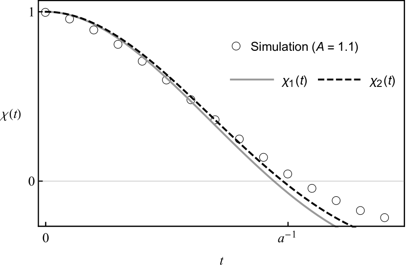
Figure 3: Local time autocorrelation function $\chi(t)$ of the time series $x_{\varepsilon}(t)$: comparison of theoretical predictions $\chi_{1}(t)$ and $\chi_{2}(t)$ [Eqs. (9) and (31)] with the simulation results with $A=1.1$. The corrections that are introduced in $\chi_{2}(t)$ by including the second-order response term in Eq. (11) provide a subtle improvement over $\chi_{1}(t)$.

Figure 4: Curve fitting of $\hat{\chi}(t)$ to the time autocorrelation function of $x_{\varepsilon}(t)$ observed in simulations with $A=1.1$. The expression optimized in the interval $0\leq t\lesssim a^{-1}$ extrapolates well up to $t\lesssim 2a^{-1}$.

Equation (9), which approximates the autocorrelation function $\chi(t)$, has been derived from the Volterra expansion truncated at the linear term $\gamma_{1}(t)$ given by Eq. (22). To find a second-order correction, one may include a quadratic contribution in $x(t)\approx\gamma_{1}(t)+\gamma_{2}(t)$:

$$\chi(t)\approx\chi_{2}(t)=\frac{\theta_{1}(t)+\theta_{2}(t)}{\theta_{1}(0)+\theta_{2}(0)},$$ (31)

in which

$$\theta_{1}(t)= -\frac{A^{2}}{4ab}\chi_{1}(t),$$ (32)

$$\theta_{2}(t)= \langle\gamma_{2}(0)\gamma_{2}(t)\rangle-\langle\gamma_{2}\rangle^{2}.$$ (33)

From (Schetzen, 2006, Eq. (11.3-14)) one can find the Fourier transform of $\theta_{2}$

$$\Theta_{2}(\omega)=\frac{A^{4}}{\pi}\int d\lambda\,|G_{2}(\lambda,\omega-\lambda)|^{2}\\ =-\frac{9bcA^{4}}{\pi}|G_{1}(\omega)|^{2}\int d\lambda\,|G_{1}(\omega)|^{2}\,|G_{1}(\omega-\lambda)|^{2}.$$ (34)

Note that

$$\theta_{1}(t)=\int\frac{d\omega}{2\pi A^{2}}|G_{1}(\omega)|^{2}\exp(\operatorname{\mathrm{i}}\omega t).$$

By virtue of the convolution theorem, the inverse Fourier transform of Eq. (34) then yields

$$\theta_{2}(t)\propto\int ds\,\chi_{1}(t-s)\chi_{1}(s)^{2}=\operatorname{\mathrm{const}}_{0}\exp(-a\,|t|)+\exp(-a\,|t|/2)\,[\;\operatorname{\mathrm{const}}_{1}\sin(\Omega\,|t|)+\operatorname{\mathrm{const}}_{2}\cos(\Omega\,|t|)\;]\\ +\exp(-a\,|t|/2)\,[\;\operatorname{\mathrm{const}}_{3}\sin(2\Omega\,|t|)+\operatorname{\mathrm{const}}_{4}\cos(2\Omega\,|t|)\;],$$ (35)

in which the unwieldy constants $\operatorname{\mathrm{const}}_{i=0,1,2,3,4}$ are not spelled out for clarity. These coefficients, which can be readily found with the help of a symbolic computational software Mat (2018), depend in a complicated manner on all four parameters of the Duffing oscillator.

The complete expression of $\chi_{2}(t)$ reveals higher-order harmonics $j\Omega,\,j=2,3...$ in the autocorrelation function. Additional oscillations at these frequencies are commensurate with the undulations of $\chi_{1}(t)$. For this reason, as noted in the main text, Eq. (10) predicts correctly the undulatory component of $\chi(t)$.

Due to the complexity of the explicit expression for $\chi_{2}(t)$, using Eq. (31) in calculations and curve fitting is problematic. The improvement that is achieved over Eq. (9) is also modest (Fig. 4). Higher-order expressions that take into account more terms from Eq. (11), might be formidably long. In curve fitting we therefore use a phenomenological Eq. (10) as justified below.

Contemplating the development of the Volterra terms in Eqs. (19)–(30), one may expect that $\chi(t)\approx\chi_{n}(t)$, calculated from Eq. (11) with $n$ response terms, contains only convolution and power products of $\chi_{1}(t)$ [cf. Eq. (35)]. The resulting expression would be a composition of time-dependent factors in the form $\propto\exp(iat/2)$, $\propto\sin(j\Omega t)$, $\propto\cos(k\Omega t)$ with integers $i\geq 2,\,j\geq 1,\,k\geq 1$. Whereas we retain the fundamental harmonic terms $\propto\sin(\Omega t)$ and $\propto\cos(\Omega t)$, as well as the slowly decaying exponential $\propto\exp(at)$ in $\chi_{2}(t)$, we introduce unknown coefficients $\alpha$ and $\beta$ to account for higher-order corrections. By imposing an additional constraint $\chi(0)=1$, we arrive at Eq. (10).

Finally, we discuss briefly the procedure of curve fitting for Eq. (10) (Fig 4). By using the criterion of Lagarkov and Sergeev Lagar’kov and Sergeev (1978); Belousov and Cohen (2016), we select from the sample autocorrelation data the observations in the interval $0\leq t\leq t_{0}$, in which $t_{0}$ is the instant when the autocorrelation function reaches the value of zero for the first time [$\chi(t_{0})=0$]. This choice of $t_{0}$ corresponds approximately to the relaxation time $t_{0}\approx\tau$, for which Eq. (10) should give accurate results. As an initial guess we recommend setting $\alpha=0$ and $\beta=0$. Otherwise the least-square fitting of Eq. (10), which is a flexible expression with four unknown parameters, may return suboptimal results.

A simple least-square fitting of the phenomenological Eq. (10) underestimates standard errors of the parameter values. We report more realistic estimates, which are recalculated by using the optimized parameter values and the uncertainty of the time autocorrelation data Bowley (1928)

$$\Delta{\chi}\approx\sqrt{\frac{1-\chi^{2}}{n-2}}.$$

IV Simulation algorithm

For computational experiments we convert Eq. (1) into an equivalent two-dimensional dynamical system ${\bm{X}}=(x,y)=(x,\dot{x})$:

$$\begin{cases}\dot{x}=y\\ \dot{y}=-ay-bx-cx^{3}+f(t).\end{cases}$$ (36)

We adopt a second-order operator-splitting approach for stochastic systems (Belousov et al., 2017, Appendix C) by decomposing the time-evolution operator $\mathcal{T}$ as

$$\dot{{\bm{X}}}=\mathcal{T}{\bm{X}}=(\mathcal{T}_{y,x}+\mathcal{T}_{x,y}+\mathcal{T}_{y,y}){\bm{X}},$$ (37)

in which

$$\mathcal{T}_{y,x}=y\partial_{x},\quad\mathcal{T}_{y,y}=-ay\partial_{y},$$

$$\mathcal{T}_{x,y}=(f-bx-cx^{3})\partial_{y}.$$

The formal solution of Eq. (37) for a time step $\Delta{t}$ is

$${\bm{X}}(t+\Delta{t})=\exp(\mathcal{T}\Delta{t}){\bm{X}}(t),$$

in which the time-evolution operator can be approximated by

$$\exp[\mathcal{T}\Delta{t}+O(\Delta{t}^{2})]=\exp\left(\frac{\mathcal{T}_{y,x}\Delta{t}}{2}\right)\exp\left(\frac{\mathcal{T}_{y,y}\Delta{t}}{2}\right)\\ \times\exp(\mathcal{T}_{x,y}\Delta{t})\exp\left(\frac{\mathcal{T}_{y,y}\Delta{t}}{2}\right)\exp\left(\frac{\mathcal{T}_{y,x}\Delta{t}}{2}\right).$$ (38)

The action of an individual operator of the form $\exp(\mathcal{L}\Delta{t})$ can be inferred by solving the simplified dynamics

$$\dot{{\bm{X}}}(t)=\mathcal{L}{\bm{X}}(t)\Rightarrow{\bm{X}}(t+\Delta{t})=\exp(\mathcal{L}\Delta{t}){\bm{X}}(t).$$ (39)

The composite operator (38) then leads to the following algorithm for the numerical integration of Eq. (37):

$$x(t+\Delta{t}/2)=x(t)+y(t)\Delta{t}/2,$$ (40)

$$y(t+\Delta{t})=y(t)\exp(-a\Delta{t})$$

$$\quad-\exp(-a\Delta{t}/2)[b+cx(t+\Delta{t}/2)^{2}]x(t+\Delta{t}/2)\Delta{t}$$

$$\quad+\exp(-a\Delta{t}/2)\int_{t}^{t+\Delta{t}}dtf(t),$$ (41)

$$x(t+\Delta{t})=x(t+\Delta{t}/2)+y(t+\Delta{t})\Delta{t}/2.$$ (42)

References

- Khan and Vyas (2001) A. A. Khan and N. S. Vyas, Nonlinear Dynamics 24, 285 (2001).
- Chatterjee and Vyas (2003) A. Chatterjee and N. S. Vyas, Journal of Vibration and Acoustics 125, 299 (2003).
- Alonso et al. (2014) R. Alonso, F. Goller, and G. B. Mindlin, Physical Review E 89 (2014), 10.1103/PhysRevE.89.032706.
- Mindlin (2017) G. B. Mindlin, Chaos: An Interdisciplinary Journal of Nonlinear Science 27, 092101 (2017).
- Cherevko et al. (2016) A. A. Cherevko, A. V. Mikhaylova, A. P. Chupakhin, I. V. Ufimtseva, A. L. Krivoshapkin, and K. Y. Orlov, Journal of Physics: Conference Series 722, 012045 (2016).
- Parshin et al. (2016) D. V. Parshin, I. V. Ufimtseva, A. A. Cherevko, A. K. Khe, K. Y. Orlov, A. L. Krivoshapkin, and A. P. Chupakhin, Journal of Physics: Conference Series 722, 012030 (2016).
- Cherevko et al. (2017) A. A. Cherevko, E. E. Bord, A. K. Khe, V. A. Panarin, and K. J. Orlov, Journal of Physics: Conference Series 894, 012012 (2017).
- Izhikevich and FitzHugh (2006) E. Izhikevich and R. FitzHugh, Scholarpedia 1, 1349 (2006).
- Strogatz (2014) S. H. Strogatz, Nonlinear Dynamics and Chaos: With Applications to Physics, Biology, Chemistry, and Engineering, 2nd ed. (Avalon Publishing, 2014).
- Chatterjee (2010) A. Chatterjee, International Journal of Mechanical Sciences 52, 1716 (2010).
- Smelyanskiy et al. (2005) V. Smelyanskiy, D. Luchinsky, D. Timuçin, and A. Bandrivskyy, Physical Review E 72 (2005), 10.1103/PhysRevE.72.026202.
- He et al. (2007) Q. He, L. Wang, and B. Liu, Chaos, Solitons & Fractals 34, 654 (2007).
- Quaranta et al. (2010) G. Quaranta, G. Monti, and G. C. Marano, Mechanical Systems and Signal Processing 24, 2076 (2010).
- Rugh (1981) W. J. Rugh, Nonlinear System Theory: The Volterra/Wiener Approach (Johns Hopkins University Press, 1981).
- Peterson (1967) R. L. Peterson, Reviews of Modern Physics 39, 69 (1967).
- Note (0) See Supplemental Material.
- Ku and Wolf (1966) Y. H. Ku and A. A. Wolf, Journal of the Franklin Institute 281, 9 (1966).
- Belousov et al. (2014) R. Belousov, P. De Gregorio, L. Rondoni, and L. Conti, Physica A: Statistical Mechanics and its Applications 412, 19 (2014).
- Belousov et al. (2016) R. Belousov, E. G. D. Cohen, C.-S. Wong, J. A. Goree, and Y. Feng, Physical Review E 93 (2016), 10.1103/PhysRevE.93.042125.
- Touchette (2009) H. Touchette, Physics Reports 478, 1 (2009).
- Chandrasekhar (1943) S. Chandrasekhar, Rev. Mod. Phys. 15, 1 (1943).
- Belousov and Cohen (2016) R. Belousov and E. G. D. Cohen, Physical Review E 94 (2016), 10.1103/PhysRevE.94.062124.
- Note (1) If one should use its absolute value instead and replace the trigonometric functions of cosine and sine in Eq. (9) by the hyperbolic ones (Belousov and Cohen, 2016; Chandrasekhar, 1943, Sec. II-3).
- Zwanzig and Ailawadi (1969) R. Zwanzig and N. K. Ailawadi, Physical Review 182, 280 (1969).
- Tuckerman et al. (1992) M. Tuckerman, B. J. Berne, and G. J. Martyna, The Journal of Chemical Physics 97, 1990 (1992).
- Belousov et al. (2017) R. Belousov, E. G. D. Cohen, and L. Rondoni, Physical Review E 96 (2017), 10.1103/PhysRevE.96.022125.
- Mat (2018) “Mathematica,” Wolfram Research, Inc. (2018).
- Note (2) We set to three standard deviations of the Gaussian approximation for Eq. (8) at the most likely values .
- Schetzen (2006) M. Schetzen, The Volterra and Wiener Theories of Nonlinear Systems (Krieger Pub., 2006).
- Lagar’kov and Sergeev (1978) A. N. Lagar’kov and V. M. Sergeev, , 24 (1978).
- Bowley (1928) A. L. Bowley, Journal of the American Statistical Association 23, 31 (1928).