Multiple Graph Adversarial Learning

Abstract

Recently, Graph Convolutional Networks (GCNs) have been widely studied for graph-structured data representation and learning. However, in many real applications, data are coming with multiple graphs, and it is non-trivial to adapt GCNs to deal with data representation with multiple graph structures. One main challenge for multi-graph representation is how to exploit both structure information of each individual graph and correlation information across multiple graphs simultaneously. In this paper, we propose a novel Multiple Graph Adversarial Learning (MGAL) framework for multi-graph representation and learning. MGAL aims to learn an optimal structure-invariant and consistent representation for multiple graphs in a common subspace via a novel adversarial learning framework, which thus incorporates both structure information of intra-graph and correlation information of inter-graphs simultaneously. Based on MGAL, we then provide a unified network for semi-supervised learning task. Promising experimental results demonstrate the effectiveness of MGAL model.

1 Introduction

Graph representation and learning which aims to represent each graph node as a low-dimensional feature vector is a fundamental problem in pattern recognition and machine learning area. Recently, Graph Convolutional Networks (GCNs) have been widely studied for graph representation and learning [6, 2, 18, 22]. These methods can be categorized into spatial and spectral methods. Spatial methods generally define graph convolution operation by designing an operator on node neighbors while spectral methods usually define graph convolution operation based on spectral analysis of graphs. For example, Monti et al. [13] present mixture model CNNs (MoNet) for graphs. Velickovic et al. [22] present Graph Attention Networks (GAT) for graph semi-supervised learning. For spectral methods, Bruna et al. [3] propose to define graph convolution based on eigen-decomposition of graph Laplacian matrix. Henaff et al. [9] further introduce a spatially constrained spectral filters. Defferrard et al. [5] propose to approximate the spectral filters based on Chebyshev expansion. Kipf et al. [11] propose a more simple Graph Convolutional Network (GCN) based on first-order approximation of spectral filters.

However, in many applications, data are coming with multiple graphs, which is known as multi-graph learning [15]. In this paper, we focus on multiple graphs that contain the common node set but with multiple different edge structures. The aim of our multi-graph representation is to find a consistent node representation across all of graphs. One main challenge for this problem is how to effectively integrate multiple graph (edge) structures together in graph node representation. The above existing GCNs generally cannot be used to deal with multiple graphs. To generalize GCNs to multiple graphs, one popular way is to use some heuristic fusion strategy and transform multi-graph learning to traditional single graph learning [17, 20, 19]. However, since the fusion process is usually independent of graph representation/learning, this strategy may lead to weak optimal solution. In addition, some works propose to conduct the convolution operation on multiple graphs by sharing the common convolution parameters across different graphs [6, 2, 25]. This mechanism can propagate some information/knowledge across multiple graphs. However, the learned representations of individual graphs in these methods are still not guaranteed to be consistent explicitly.

In this paper, we propose a novel Multiple Graph Adversarial Learning (MGAL) framework for multi-graph representation and learning. MGAL aims to learn an optimal structure-invariant and thus consistent representation for multiple graphs in a common subspace via an adversarial learning architecture. Based on MGAL, we further provide a unified network for multi-graph based semi-supervised learning task. Overall, the main contributions of this paper are summarized as follows:

• We propose a novel Multiple Graph Adversarial Learning (MGAL) framework for multi-graph representation and learning. The proposed MGAL is a general framework which allows to generalize any learnable/parameterized graph representation models to deal with multiple graphs.

• We present a unified network for semi-supervised learning task based on multi-graph representation.

• We develop a general generative adversarial learning architecture (‘multiple generators + one discriminator’) to address the general multi-view representation and learning problem.

Experimental results on several datasets demonstrate the effectiveness and benefits of the proposed MGAL model and semi-supervised learning method.

2 Problem Formulation

Graph representation. Let $G(X,A)$ be an attributed graph where $X=(x_{1},x_{2}\cdots x_{n})\in\mathbb{R}^{n\times d}$ denotes the collection of node features and $A\in\mathbb{R}^{n\times n}$ encodes the pairwise relationships (such as similarities) between node pairs. The aim of graph representation is to learn a latent representation $Z=f(X,A;\Theta)$ where $Z=(z_{1}\cdots z_{n})\in\mathbb{R}^{n\times k},k\leq d$ in a low-dimensional space that takes in both graph structure $A$ and node content $X$ together. One kind of popular way is to use Graph Convolutional Networks (GCNs) [11, 22, 9, 13] which provide a unified framework to define the representation function $f(X,A;\Theta)$. Based on representation $Z$, we can then conduct some learning tasks, such as node classification, clustering and semi-supervised classification, etc.

Multi-graph representation. In many real applications, data are coming with multiple graphs, which is known as multi-graph representation/learning problem. In this paper, we focus on multiple graphs that contain the common node set and the same node content but with multiple different edge structures. Formally, given $G(X,\mathcal{A})$ with $X\in\mathbb{R}^{n\times d}$ denoting node content and $\mathcal{A}=\{A^{(1)},A^{(1)}\cdots A^{(m)}\}$ representing the multiple edge structures, the aim of our multi-graph representation is to learn a consistent latent representation $Z=h(X,\mathcal{A};\Theta)$, where $Z\in\mathbb{R}^{n\times k},k\leq d$ in a low-dimensional space that takes in multiple graph structures $\mathcal{A}$ and node content $X$ together. Based on representation $Z$, we can then conduct some learning tasks, such as node classification, clustering and semi-supervised learning, etc. In this paper, we focus on semi-supervised learning. The main challenge for multi-graph representation is how to exploit the information of each individual graph $A^{(v)}$ while take in the correlation cue among multiple graphs simultaneously in final representation $Z$. A simple and direct way to use multiple graphs is to average them to a new one and then put it into the standard GCNs model. Obviously, since the graph average process is independent of graph learning, this may lead to weak local optimal solution.

3 Related Works

Multiple graph convolutional representation. To generalize GCNs to multiple graphs, one can first obtain the representation $Z^{(v)}=f(X,A^{(v)};\Theta^{(v)})$ for each graph $A^{(v)}$ individually by using GCNs and then concatenate or average them together to obtain the final representation $Z$. Obviously, this two-stage strategy neglects the correlation information among different graphs. To overcome this issue, some works propose to conduct ensemble of different representations in middle layers of GCNs to share/communicate some information across different graphs in learning process [17, 20, 19]. Since the fusion in each layer is independent of graph learning, this strategy may still lead to weak optimal representation.

Another kind of works propose to conduct the convolution operation on multiple graphs by sharing the common convolution parameters across different graphs, i.e., $Z^{(v)}=f(X,A^{(v)};\Theta)$ [6, 2, 25]. This mechanism can propagate some correlation information across graphs $A^{(v)},v=1\cdots m$ via the common parameters $\Theta$. However, although the parameters $\Theta$ are common for different graphs, the learned representations $\{Z^{(1)}\cdots Z^{(m)}\}$ are still not guaranteed to be well consistent because each $Z^{(v)}=f(X,A^{(v)};\Theta)$ is determined by not only parameters $\Theta$ but also individual graph $A^{(v)}$.

Adversarial learning model. Our multiple graph adversarial learning model is inspired by Generative Adversarial Network (GAN) [8], which consists of a generator $\mathcal{G}$ and a discriminator $\mathcal{D}$. The generator is trained to generate the samples to convince the discriminator while the discriminator aims to discriminate the samples returned by generator. Recently, adversarial learning has been explored in graph representation tasks. Wang et al. [23] propose a graph representation model with GANs (GraphGAN). Dai et al. [4] propose an adversarial network embedding (ANE), which employs the adversarial learning to regularize graph representation. Pan et al. [16] also propose an adversarially regularized graph autoencoder model for graph embedding.

Different from previous works, our aim in this paper is to derive a general adversarial learning framework for multiple graph representation and learning. To the best of our knowledge, it is the first effort to develop adversarial learning framework for multi-graph learning problem.

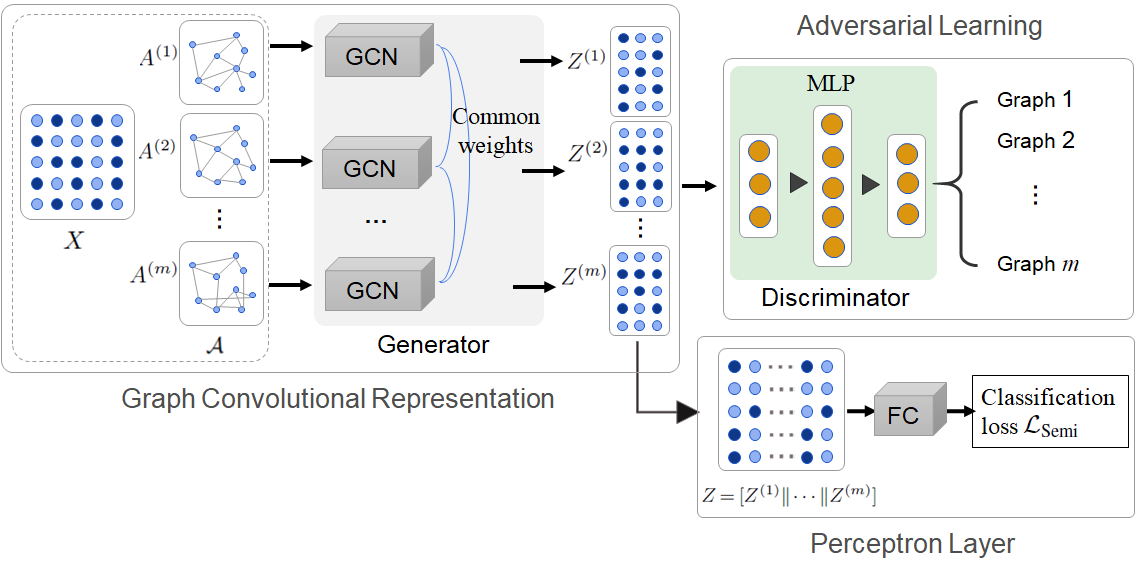
Figure 1: Architecture of the proposed multiple graph adversarial learning. It consists of three main modules, i.e., graph convolutional representation, adversarial learning network and perceptron layer for node label prediction.

4 The Proposed Model

4.1 Overall Framework

Given an input feature matrix $X$ and associated multiple graph structures $\mathcal{A}=\{A^{(1)}\cdots A^{(m)}\}$, our aim is to learn a consistent latent representation $Z=h(X,\mathcal{A};\Theta)$ and then conduct graph node semi-supervised classification in a unified network model. Figure 1 demonstrates the overall architecture of our Multiple Graph Adversarial Learning (MGAL) which consists of three main modules, i.e., graph convolutional representation, adversarial learning module and perceptron layer for node label prediction.

• Graph convolutional representation. We employ several graph convolutional layers to learn a latent low-dimensional representation $Z^{(v)}$ for each individual graph by incorporating both structure of graph $A^{(v)}$ and node features $X$ together.

• Adversarial learning. The adversarial learning module aims to enforce the latent representations $Z^{(v)}$ of graphs to be consistent and generate a kind of structure-invariant representations for different graphs ${A}^{(v)}$ in a common subspace.

• Perceptron layer. We obtain the final representation $Z$ by concatenating $Z^{(v)}$ together and use a perceptron layer to predict the label for each node, and thus conduct semi-supervised classification for graph nodes.

4.2 Graph Convolutional Representation

The graph convolutional representation aims to learn a latent representation $Z^{(v)}=f(X,A^{(v)};\Theta)$ for nodes of each graph by exploring both structure of graph $A^{(v)}$ and node feature $X$ together. In this paper, we propose to employ graph convolutional networks (GCNs) [11, 6, 2] which have been widely studied in recent years. The main property of GCNs architecture is that it can represent both graph structure $A^{(v)}$ and node content $X$ in a unified framework. Generally, given a graph $G(X,A)$, GCNs conduct layer-wise propagation in hidden layers as

$$H^{(v)}_{l+1}=f_{l}(H^{(v)}_{l},A^{(v)};\Theta_{l})$$ (1)

where $l=0,1\cdots L-1,v=1,2\cdots m$ and $L$ is the number of layers. $H^{(v)}_{0}=X\in\mathbb{R}^{n\times d}$ is the initial input feature matrix. $H^{(v)}_{l}$ denotes the input feature map of the $l$-th layer and $H^{(v)}_{l+1}$ is the output feature representation after conducting graph convolutional operation on graph $A^{(v)}$. Parameters $\Theta=\{\Theta_{0}\cdots\Theta_{L-1}\}$ are layer-specific trainable weight matrices needing to be learned. We can thus use the final output of GCNs as a compact representation for each individual graph $A^{(v)}$ as

$$Z^{(v)}=f(X,A^{(v)};\Theta)=H^{(v)}_{L}$$ (2)

Many methods have been proposed to provide various kinds of graph convolution operator $f_{l}$ in recent years. In this paper, we employ the widely used spectral convolution function [11] defined as

$$f_{l}(H^{(v)}_{l},A^{(v)};\Theta_{l})=\sigma\big{(}{D^{(v)}}^{-\frac{1}{2}}\tilde{A}^{(v)}{D^{(v)}}^{-\frac{1}{2}}H^{(v)}_{l}\Theta_{l}\big{)}$$

where $\tilde{A}^{(v)}=A^{(v)}+I$ and $D^{(v)}=\sum^{n}_{j=1}\tilde{A}^{(v)}_{ij}$. $I$ is the identity matrix and $\sigma$ denotes an activation function, such as $\textrm{ReLU}(\cdot)=\max(0,\cdot)$.

Remark. Note that, in our graph convolutional architecture, the weight parameters $\Theta=\{\Theta_{0}\cdots\Theta_{L}\}$ of hidden layers for different graphs are shared which can thus propagate some information/knowledge across different graphs for node representation, as suggested in works [6, 2].

4.3 Adversarial Learning

As mentioned in §2, for our multi-graph learning problem, it is necessarily to generate a consistent representation across different graphs in a common subspace. However, the above learned representations $Z^{(v)}$ (Eq.(2)) can not be guaranteed to be consistent because $Z^{(v)}$ is determined by not only the common shared parameters $\Theta$ but also individual graph $A^{(v)}$. To overcome this issue, we design an adversarial learning module, which consists of a generator and a discriminator [8]. Our adversarial model is built on a standard multi-layer perceptron (MLP), which acts as a discriminator to distinguish whether the representation $Z^{(v)}$ is generated from graph $A^{(v)}$ or some other graph $A^{(u)}$ where $u\neq v$.

Generator $\mathcal{G}(X,A^{(v)};\Theta)$ aims to generate a kind of structure-invariant/consistent representations $Z^{(v)}$ for graphs $A^{(v)}$ in a common subspace. In this paper, we employ the above GCNs as our generator module, i.e.,

$$Z^{(v)}=\mathcal{G}(X,A^{(v)};\Theta)=f(X,A^{(v)};\Theta)$$ (3)

For each node representation, we denote

$$z^{(v)}=\mathcal{G}(x,A^{(v)};\Theta)=f(x,A^{(v)};\Theta)$$ (4)

where $x\in X$ is the input feature vector of a graph node and $z^{(v)}\in Z^{(v)}$ is the corresponding generated representation. The generator is supervised and optimized by both cross-graph discrimination loss and node (semi-supervised) classification loss. The cross-graph discrimination loss minimizes the gap among different graph representations (as shown in Eq.(5)) while the classification loss can separate the representations of graph nodes for node semi-supervised classification task (as shown in Eq.(7)).

Discriminator $\mathcal{D}(Z)$ aims to discriminate the representation $Z$ obtained from the generator. It is built on a standard multi-layer perceptron (MLP) and defined as a multi-class classifier. It outputs a class label indication vector $\mathcal{D}(Z)=(\mathcal{D}^{(1)}(Z)\cdots\mathcal{D}^{(m)}(Z))$ in which $\mathcal{D}^{(v)}(Z)$ represents the probability of representation $Z$ generating from the $v$-th graph $A^{(v)}$ and $\sum^{m}_{v=1}\mathcal{D}^{(v)}(Z)=1,\mathcal{D}^{(v)}(Z)\geq 0$.

In our adversarial learning, generator $\mathcal{G}$ and discriminator $\mathcal{D}$ act as two opponents. Generator $\mathcal{G}$ would try to generate an indistinctive representation $Z^{(v)}$ for each graph $A^{(v)}$, while discriminator $\mathcal{D}$, on the contrary, would try to discriminate whether the representation $Z^{(v)}$ is generated from the $v$-th graph or some other graph. This can be achieved by optimizing the following cross-entropy loss $\mathcal{L}_{\mathrm{MGAL}}$ as

$$\min_{\mathcal{G}}\max_{\mathcal{D}}\mathcal{L}_{\mathrm{MGAL}}=\frac{1}{m}\sum^{m}_{v=1}\Big{(}\mathbb{E}_{x}\log\big{[}\mathcal{D}^{(v)}(\mathcal{G}(x,A^{(v)};\Theta))\big{]}$$

$$+\textstyle\frac{1}{m-1}\sum^{m}_{u,u\neq v}\mathbb{E}_{x}\log\big{[}1-\mathcal{D}^{(u)}(\mathcal{G}(x,A^{(v)};\Theta))\big{]}\Big{)}$$ (5)

Remark. In our MGAL, since the convolutional parameters $\Theta$ are shared for multiple graphs $G(X,A^{(v)})$, thus only one generator is designed. Note that, here one can also use multiple generators $\mathcal{G}(X,A^{(v)},\Theta^{(v)})$ with each generator conducting on each individual graph respectively. This ‘multiple generators + one discriminator’ adversarial learning provides a new feasible architecture to address the general multi-graph (view) representation and learning tasks.

4.4 Perceptron Layer

After adversarial training, all the representation $Z^{(v)},v=1,2\cdots m$ are lied in a common low-dimensional space. In the final perceptron layer, we can use one of them or aggregate them for the final node representation. In this paper, we first aggregate $\{Z^{(1)}\cdots Z^{(m)}\}$ by concatenating them as $Z=[Z^{(1)}\|Z^{(2)}\cdots\|Z^{(m)}]\in\mathbb{R}^{n\times md}$ where $\|$ denotes the concatenation operation and then employ a fully-connected layer to conduct label prediction as

$$U=\mathrm{softmax}(ZW)$$ (6)

where $W\in\mathbb{R}^{md\times c}$ is a trainable weight matrix and $c$ denote the number of node classes. The final output $U\in\mathbb{R}^{n\times c}$ denotes the predicted label vectors for graph nodes. Note that, here one can also use a graph convolutional layer to conduct label prediction as

$$U=\mathrm{softmax}(\bar{A}ZW)$$ (7)

where $\bar{A}=\frac{1}{m}\sum^{m}_{v=1}A^{(v)}$. For semi-supervised learning, we aim to minimize the following cross-entropy loss $\mathcal{L}_{\textrm{Semi}}$ over all the labeled nodes $L$, i.e.,

$$\mathcal{L}_{\textrm{Semi}}=-\sum\nolimits_{i\in L}\sum^{c}\nolimits_{j=1}{Y}_{ij}\log{U}_{ij}$$ (8)

where ${L}$ indicates the set of labeled nodes and ${Y}_{i\cdot},i\in L$ denotes the corresponding label indication vector for the $i$-th labeled node, i.e.,

$${Y}_{ij}=\begin{cases}1&\text{if node $i$ belongs to $j$-th class}\\ 0&\text{otherwise}\end{cases}$$ (9)

Figure 2 demonstrates the 2D t-SNE [21] visualization of the representation output by GCN on each individual graph $A^{(v)}$ (denote as GCN(v)) and MGAL on multiple graph $\mathcal{A}$ respectively on MSRC-v1 dataset [24] (as shown in Experiments). Different colors denote different classes. Intuitively, one can observe that the data of different classes are distributed more clearly in MGAL representation, which demonstrates the benefits of MGAL on conducting multi-graph representation and learning.

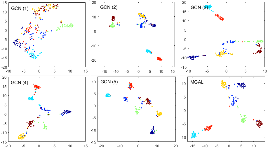
Figure 2: 2D t-SNE [21] visualizations of the representation based on GCN and MGAL, respectively on MSRC-v1 dataset. Different classes are marked by different colors. Note that, comparing with traditional single graph GCN, the data distribution is demonstrated more clearly in our multi-graph representation.

Table 1: Comparison results of semi-supervised classification on Handwritten numerals, Caltech101-7, MSRC-v1 and CiteSeer datasets, respectively. The best performance are marked by bold.

Dataset	Handwritten numerals			Caltech101-7
Ratio of label	10%	20%	30%	10%	20%	30%
GCN(1)	85.88$\pm$0.91	87.51$\pm$0.77	87.65$\pm$0.60	83.55$\pm$0.81	84.12$\pm$1.26	84.18$\pm$1.37
GCN(2)	93.32$\pm$1.41	95.33$\pm$0.49	95.66$\pm$0.51	82.09$\pm$0.40	83.59$\pm$0.59	85.45$\pm$1.39
GCN(3)	95.14$\pm$0.66	96.71$\pm$0.47	97.17$\pm$0.51	84.92$\pm$0.78	86.18$\pm$2.34	86.56$\pm$1.85
GCN(4)	95.26$\pm$0.93	97.19$\pm$0.22	97.46$\pm$0.50	93.20$\pm$1.01	95.06$\pm$0.59	95.76$\pm$0.77
GCN(5)	84.61$\pm$0.38	96.71$\pm$0.48	86.40$\pm$0.64	91.64$\pm$1.91	92.47$\pm$3.04	94.18$\pm$2.24
GCN(6)	71.01$\pm$1.87	71.44$\pm$1.69	73.03$\pm$1.28	90.45$\pm$1.98	92.36$\pm$2.09	94.27$\pm$0.87
GCN-M	95.89$\pm$0.67	95.85$\pm$2.48	97.38$\pm$0.63	90.01$\pm$2.44	92.42$\pm$2.87	93.87$\pm$1.55
Multi-GCN	96.89$\pm$0.35	97.47$\pm$0.38	97.89$\pm$0.29	93.75$\pm$2.32	95.60$\pm$0.82	95.28$\pm$3.01
AMGL	91.82$\pm$0.55	94.15$\pm$0.32	95.65$\pm$0.73	88.83$\pm$0.69	92.79$\pm$0.34	94.62$\pm$0.42
MLAN	97.32$\pm$0.23	97.48$\pm$0.19	97.91$\pm$0.28	93.52$\pm$0.58	94.84$\pm$0.19	95.46$\pm$0.18
MGAL	97.64$\pm$0.39	98.25$\pm$0.34	98.48$\pm$0.42	95.00$\pm$1.07	96.41$\pm$0.81	97.14$\pm$0.44
Dataset	MSRC-v1			CiteSeer
Ratio of label	10%	20%	30%	10%	20%	30%
GCN(1)	42.75$\pm$11.2	45.09$\pm$4.45	45.00$\pm$7.38	71.08$\pm$1.83	75.62$\pm$1.14	77.95$\pm$1.59
GCN(2)	77.69$\pm$8.15	83.98$\pm$2.47	83.43$\pm$5.45	73.38$\pm$2.89	77.44$\pm$1.16	79.15$\pm$0.96
GCN(3)	81.21$\pm$4.52	84.84$\pm$1.65	89.57$\pm$2.15	-	-	-
GCN(4)	70.66$\pm$2.77	75.65$\pm$2.87	76.00$\pm$4.49	-	-	-
GCN(5)	71.10$\pm$4.64	78.88$\pm$5.39	79.57$\pm$2.84	-	-	-
GCN-M	80.77$\pm$4.13	86.21$\pm$3.37	90.29$\pm$2.15	72.84$\pm$2.32	77.93$\pm$1.49	80.13$\pm$1.82
Multi-GCN	83.30$\pm$2.21	88.70$\pm$1.69	89.29$\pm$2.43	72.04$\pm$1.37	76.15$\pm$1.42	77.69$\pm$1.73
AMGL	82.29$\pm$2.43	89.35$\pm$2.09	90.21$\pm$1.08	64.78$\pm$1.58	68.00$\pm$1.41	70.92$\pm$2.93
MLAN	83.66$\pm$2.38	87.92$\pm$1.18	89.47$\pm$1.68	63.24$\pm$6.54	59.49$\pm$6.72	60.47$\pm$6.16
MAGL	88.68$\pm$0.66	89.93$\pm$2.40	91.29$\pm$1.65	75.18$\pm$1.64	78.84$\pm$1.57	78.77$\pm$1.25

5 Experiments

To evaluate the effectiveness of the proposed MGAL and semi-supervised learning method, we implement it and compare it with some other methods on four datasets.

5.1 Datasets

We test our MGAL on four datasets including MSRC-v1 [24], Caltech101-7 [12, 15], Handwritten numerals [1] and CiteSeer [1]. The details of these datasets and their usages in our experiments are introduced below.

MSRC-v1 dataset [24] contains 8 classes of 240 images. Following [15], in our experiments, we select 7 classes including tree, building, airplane, cow, face, car and bicycle. Each class contains 30 images. Following the experimental setting in work [15], five graphs are obtained for this dataset by using five different kinds of visual descriptors, i.e., 24 Color Moment, 576 Histogram of Oriented Gradient, 512 GIST, 256 Local Binary Pattern and 254 Centrist features.

Caltech101-7 dataset [12, 15] is an object recognition data set containing 101 categories of images. We follow the experimental setup of previous work [14] and select the widely used 7 classes (Dolla-Bill, Face, Garfield, Motorbikes, Snoopy, Stop-Sign and Windsor-Chair) and obtain 1474 images in our experiments. Six neighbor graphs are obtained for this dataset by using six different kinds of visual feature descriptors including 48 dimension Gabor feature, 40 dimension wavelet moments (WM), 254 dimension CENTRIST feature, 1984 dimension HOG feature, 512 dimension GIST feature, and 928 dimension LBP feature.

Handwritten numerals [1] dataset contains 2,000 data points for 0 to 9 ten digit classes and each class has 200 data points. We construct six graphs by using six published feature descriptors including 76 Fourier coefficients of the character shapes, 216 profile correlations, 64 Karhunen-love coefficients, 240 pixel averages in $2\times 3$ windows, 47 Zernike moment and morphological features.

CiteSeer dataset [1] consists of 3,312 documents on scientific publications, which can be further classified into six classes, i.e., Agents, AI, DB, IR, ML and HCI. For our multi-graph learning, two graphs are built up by using a 3,703-dimensional vector representing whether the key words are included for the text view and the other 3279-dimensional vector recording the citing relations between every two documents, respectively [15].

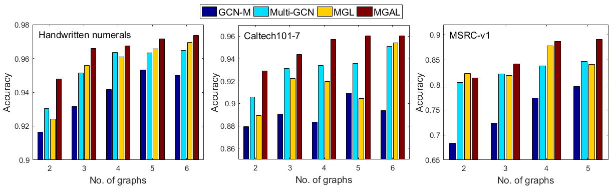
Figure 3: Comparison results on different numbers of graphs.

5.2 Experimental Setup

Parameter setting. For generator, we use a three-layer graph convolutional network and the number of units in each hidden layer is set to 64 and 16, respectively. For discriminator, we use a four-layer full connection network with the number of units in each layer is set to 16, 64, 16 and $m$ respectively where $m$ denotes the number of graphs, as discussed in §4.3. We train our generator for a maximum of 500 epochs by using Adam [10] with learning rate 0.005. We train our discriminator for a maximum of 500 epochs by using Stochastic Gradient Descent (SGD) with learning rate 0.01. All the network weights are initialized using Glorot initialization [7]. We stop training if the validation loss does not decrease for 50 consecutive epochs.

Data setting. For all datasets, we select 10%, 20% and 30% nodes as label data per class and use the remaining data as unlabeled samples. For unlabeled samples, we also use 5% nodes for validation purpose to determine the convergence criterion, as suggested in [11], and use the remaining 85%, 75% and 65% nodes respectively as test samples. All the accuracy results are averaged over 5 runs with different data splits.

Baselines. We compare our method (MGAL) against state-of-the art methods as follows,

GCN(v) that conducts traditional graph convolutional network [11] on the $v$-th graph $A^{(v)}$ and node content features $X$.
GCN-M that conducts traditional graph convolutional network [11] on the averaged graph $\bar{A}=\frac{1}{m}\sum^{m}_{v=1}A^{(v)}$ and node features $X$.
Multi-GCN that first learns representation for multiple graphs $A^{(v)}$ by using/sharing the common parameters, as suggested in work [6], and then select the representation $Z^{(v)}$ with the lowest training loss function for the final multi-graph representation.
MGL that removes the adversarial learning module in our MGAL network. We implement it as a baseline to demonstrate the effectiveness of the proposed adversarial learning.

In addition, we also compare our method with some other recent traditional multiple graph learning and semi-supervised learning methods including:

AMGL [15] is a parameter-free auto-weighted multiple graph learning and label propagation for semi-supervised learning problem.
MLAN [14] is a multi-view learning model for semi-supervised classification.

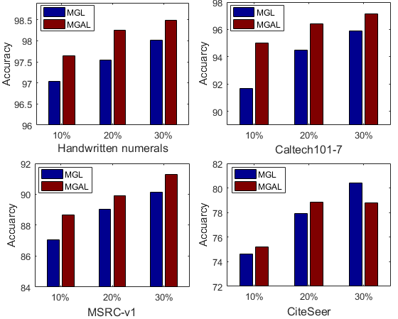
Figure 4: Comparison results of our MGAL with the baseline MGL. Note that, MGAL performs better than MGL, indicating the effectiveness of the proposed adversarial learning.

5.3 Comparison Results

Table 1 summarizes the comparison results of semi-supervised classification on four datasets. Here, one can note that (1) The proposed MGAL performs obviously better than traditional single GCN method conduced on each individual graph $A^{(v)}$. This clearly demonstrates the benefit of the proposed multi-graph representation and semi-supervised learning on multiple graphs. (2) Comparing with the other baseline method GCN-M and Multi-GCN, the proposed MGAL returns the best performance, which indicates the effectiveness of the proposed multi-graph representation architecture. (3) MGAL performs better than recent multiple graph learning and semi-supervised learning method AMGL [15] and MLAN [14], which indicates the benefit of the proposed multi-graph learning and semi-supervised learning model.

Figure 3 shows the classification accuracy of the proposed MGAL method across different numbers of graphs. For each graph number, we conduct semi-supervised experiments on all possible graph groups and then compute the average performance. Here, one can note that, (1) as the number of graphs increases, MGAL obtains better learning performance. It clearly demonstrates the desired ability of MGAL on multiple graph integration for robust learning which is the main issue for multi-graph learning task. (2) Our MGAL performs consistently better than other baseline methods on different sizes of graph set, which further indicates the advantage of the proposed MGAL.

Figure 4 shows the classification accuracy of the proposed MGAL method comparing with the baseline method MGL on four datasets. One can note that, MGAL generally performs better than MGL on all experiments, which clearly indicates the desired benefits of the proposed method by incorporating the adversarial learning architecture in multi-graph representation and learning.

6 Conclusion

This paper proposes a novel Multiple Graph Adversarial Learning (MGAL) framework for multi-graph representation and learning. MGAL aims to learn an optimal structure-invariant and thus consistent representation for multiple graphs in a common subspace, and thus incorporates both structure information of intra-graph and correlation information of inter-graphs simultaneously. Based on MGAL, we then provide a unified network for semi-supervised learning task. Promising experimental results demonstrate the effectiveness of the proposed MGAL model. The proposed MGAL is a general framework which allows to generalize any learnable/parameterized graph representation models to deal with multiple graphs.

References

- [1] D. N. Arthur Asuncion. Uci machine learning repository. 2007.
- [2] J. Atwood and D. Towsley. Diffusion-convolutional neural networks. In Advances in Neural Information Processing Systems, pages 1993–2001, 2016.
- [3] J. Bruna, W. Zaremba, A. Szlam, and Y. LeCun. Spectral networks and locally connected networks on graphs. In International Conference on Learning Representations, 2014.
- [4] Q. Dai, Q. Li, J. Tang, and D. Wang. Adversarial network embedding. In AAAI Conference on Artificial Intelligence, 2018.
- [5] M. Defferrard, X. Bresson, and P. Vandergheynst. Convolutional neural networks on graphs with fast localized spectral filtering. In Advances in Neural Information Processing Systems, pages 3844–3852, 2016.
- [6] D. K. Duvenaud, D. Maclaurin, J. Iparraguirre, R. Bombarell, T. Hirzel, A. Aspuru-Guzik, and R. P. Adams. Convolutional networks on graphs for learning molecular fingerprints. In Advances in Neural Information Processing Systems, pages 2224–2232, 2015.
- [7] X. Glorot and Y. Bengio. Understanding the difficulty of training deep feedforward neural networks. In International conference on artificial intelligence and statistics, pages 249–256, 2010.
- [8] I. Goodfellow, J. Pouget-Abadie, M. Mirza, B. Xu, D. Warde-Farley, S. Ozair, A. Courville, and Y. Bengio. Generative adversarial nets. In Advances in neural information processing systems, pages 2672–2680, 2014.
- [9] M. Henaff, J. Bruna, and Y. LeCun. Deep convolutional networks on graph-structured data. arXiv preprint arXiv:1506.05163, 2015.
- [10] D. P. Kingma and J. Ba. Adam: A method for stochastic optimization. In International Conference on Learning Representations, 2015.
- [11] T. N. Kipf and M. Welling. Semi-supervised classification with graph convolutional networks. arXiv preprint arXiv:1609.02907, 2016.
- [12] Y. Li, F. Nie, H. Huang, and J. Huang. Large-scale multi-view spectral clustering via bipartite graph. In AAAI, pages 2750–2756, 2015.
- [13] F. Monti, D. Boscaini, J. Masci, E. Rodola, J. Svoboda, and M. M. Bronstein. Geometric deep learning on graphs and manifolds using mixture model cnns. In IEEE Conference on Computer Vision and Pattern Recognition, pages 5423–5434, 2017.
- [14] F. Nie, G. Cai, and X. Li. Multi-view clustering and semi-supervised classification with adaptive neighbours. In AAAI, pages 2408–2414, 2017.
- [15] F. Nie, J. Li, X. Li, et al. Parameter-free auto-weighted multiple graph learning: A framework for multiview clustering and semi-supervised classification. In IJCAI, pages 1881–1887, 2016.
- [16] S. Pan, R. Hu, G. Long, J. Jiang, L. Yao, and C. Zhang. Adversarially regularized graph autoencoder. In International Joint Conference on Artificial Intelligence, 2018.
- [17] T. Pham, T. Tran, D. Q. Phung, and S. Venkatesh. Column networks for collective classification. In AAAI, pages 2485–2491, 2017.
- [18] F. Z. J. H. Ruoyu Li, Sheng Wang. Adaptive graph convolutional neural networks. In AAAI Conference on Artificial Intelligence, pages 3546–3553, 2018.
- [19] M. Schlichtkrull, T. N. Kipf, P. Bloem, R. van den Berg, I. Titov, and M. Welling. Modeling relational data with graph convolutional networks. In European Semantic Web Conference, pages 593–607, 2018.
- [20] M. Simonovsky and N. Komodakis. Dynamic edge-conditioned filters in convolutional neural networks on graphs. In 2017 IEEE Conference on Computer Vision and Pattern Recognition (CVPR), pages 29–38, 2017.
- [21] L. van der Maaten and G. Hinton. Visualizing data using t-sne. Journal of Machine Learning Research, pages 2579–2605, 2008.
- [22] P. Velickovic, G. Cucurull, A. Casanova, A. Romero, P. Lio, and Y. Bengio. Graph attention networks. arXiv preprint arXiv:1710.10903, 2017.
- [23] H. Wang, J. Wang, J. Wang, M. Zhao, W. Zhang, F. Zhang, X. Xie, and M. Guo. Graphgan: Graph representation learning with generative adversarial nets. In AAAI Conference on Artificial Intelligence, 2018.
- [24] J. Winn and N. Jojic. Locus: Learning object classes with unsupervised segmentation. In Computer Vision, 2005. ICCV 2005. Tenth IEEE International Conference on, volume 1, pages 756–763, 2005.
- [25] C. Zhuang and Q. Ma. Dual graph convolutional networks for graph-based semi-supervised classification. In World Wide Web Conference on World Wide Web, pages 499–508, 2018.