Multiwavelength campaign on Mrk 509

Abstract

Aims. To elucidate the location, physical conditions, mass outflow rate, and kinetic luminosity of the outflow from the active nucleus of the Seyfert 1 galaxy Mrk 509 we used coordinated ultraviolet and X-ray spectral observations in 2012 to followup our lengthier campaign conducted in 2009.

Methods. We observed Mrk 509 with the Cosmic Origins Spectrograph (COS) on the Hubble Space Telescope (HST) on 2012-09-03 and 2012-10-11 coordinated with X-ray observations using the High Energy Transmission Grating on the Chandra X-ray Observatory. Our far-ultraviolet spectra used grating G140L on COS to cover wavelengths from 920–2000 Å at a resolving power of $\sim 2000$, and gratings G130M and G160M to cover 1160–1750 Å at a resolving power of $\sim 15,000$.

Results. We detect variability in the blue-shifted UV absorption lines on timescales spanning 3–12 years. The inferred densities in the absorbing gas are greater than log $n\rm\leavevmode\nobreak\ cm^{-3}\sim 3$. For ionization parameters ranging over log $U=-1.5\rm\leavevmode\nobreak\ to\leavevmode\nobreak\ -0.2$, we constrain the distances of the absorbers to be closer than 220 pc to the active nucleus.

Conclusions. The impact on the host galaxy appears to be confined to the nuclear region.

1 Introduction

As one of the brightest Seyfert galaxies ($m_{V}=13.5$ McAlary et al. (1983); $z=0.034397$ Fisher et al. (1995)), Mrk 509 has been the target of many campaigns to understand its physical characteristics in greater detail as an aid to understanding the physics of active galactic nuclei (AGN) in general. With a bolometric luminosity of $\rm M_{bol}=2.3\times 10^{45}\leavevmode\nobreak\ \rm erg\leavevmode\nobreak\ s^{-1}$ (Runnoe et al., 2012), it lies on the Seyfert/quasar classification boundary (Kopylov et al., 1974). Campaigns with the International Ultraviolet Explorer (IUE) established its ultraviolet variability (Chapman et al., 1985). Ground-based reverberation mapping using optical spectra (Peterson et al., 1998; Kaspi et al., 2000; Peterson et al., 2004) established a black-hole mass of $1.1\times 10^{8}\leavevmode\nobreak\ M_{\odot}$ (Bentz & Katz, 2015). The earliest IUE observations (Wu et al., 1980; York et al., 1984) revealed the blue-shifted ultraviolet absorption characteristic of AGN outflows. These features were studied at more detail and at higher spectral resolution with the Far Ultraviolet Spectroscopic Explorer (FUSE) (Kriss et al., 2000) and the Space Telescope Imaging Spectrograph (STIS) on the Hubble Space Telescope (HST) (Kraemer et al., 2003). Blue-shifted absorption indicative of outflowing gas also appears in X-ray spectra (Yaqoob et al., 2003).

Table 1: COS Observations of Mrk 509

Data Set Name	Grating/Tilt	Date	Start Time	Start Time	Exposure Time
			(GMT)	(MJD)	(s)
lc0t01010	G130M/1309	2012-09-03	10:01:30	56173.417713	1642
lc0t01020	G160M/1577	2012-09-03	10:36:09	56173.441775	2707
lc0t01030	G140L/1280	2012-09-03	13:00:12	56173.541810	5041
lc0t02010	G130M/1309	2012-10-11	12:25:24	56211.517643	1642
lc0t02020	G160M/1577	2012-10-11	13:00:03	56211.541706	2707
lc0t02030	G140L/1280	2012-10-11	15:24:09	56211.641775	5041

The galaxy-wide nature of this outflow is manifested by extended, blue-shifted emission from [O iii] in optical long-slit spectra (Phillips et al., 1983), HST images (Fischer et al., 2015), and ground-based integral-field unit (IFU) observations (Liu et al., 2015). Such outflows powered by the central AGN are often invoked in models of galaxy formation in order to ameliorate several related issues. Feedback instigated by an outflow may suppress star formation or even expel gas from the host galaxy (Silk & Rees, 1998; King, 2003; Ostriker et al., 2010; Soker, 2010; Faucher-Giguère & Quataert, 2012; Zubovas & Nayakshin, 2014; Thompson et al., 2015). This in turn can link the properties of the host galaxy to those of its central black hole leading to the correlation between the black-hole mass and the central velocity dispersion of the galaxy bulge (Di Matteo et al., 2005; Hopkins & Elvis, 2010). These models require the outflow to tap into 0.5–5% of the luminosity radiated by the AGN. Measuring the mass flux and the kinetic luminosity of the outflow is therefore central to testing such models of feedback. This, in turn, requires knowledge of the location and physical conditions in the outflow.

In 2009 we undertook an extensive monitoring campaign on Mrk 509 using XMM-Newton, Chandra, HST, Swift, and INTEGRAL (Kaastra et al., 2011). This campaign established the location of several of the components of the UV outflow (Kriss et al., 2011; Arav et al., 2012) and the X-ray absorbers (Kaastra et al., 2012). The UV absorbers are characterized by seven discrete velocity components ranging from $-700$ to $+200\leavevmode\nobreak\ \rm km\leavevmode\nobreak\ s^{-1}$ relative to the systemic velocity of the host galaxy. Arav et al. (2012) set lower limits of 100–200 pc for the location of these absorbers. The X-ray absorbers lie in the same velocity range, and they comprise six distinct components in velocity and ionization state with total column densities of $\rm 0.8-6.3\times 10^{20}\leavevmode\nobreak\ cm^{-2}$ (Detmers et al., 2011). Kaastra et al. (2012) showed that the X-ray absorbers lie at distances ranging from 5 pc to 3 kpc.

In this paper we describe a longer-timescale continuation of our original monitoring program. In the fall of 2012 we obtained additional COS spectra of Mrk 509, including far-UV optimized grating tilts that yield spectra down to the galactic Lyman limit. These spectra overlap the wavelength range of the original FUSE spectra (Kriss et al., 2000, 2011). These observations were coordinated with Chandra HETGS spectra, previously discussed by Kaastra et al. (2014). In this paper we describe our COS observations and our data reduction methods in §2. §3 compares these new spectra to those from prior campaigns. §4 discusses the implications of our new observations, focusing in particular on more distant absorbing gas that exhibits longer-term variability. §5 summarizes our results.

2 Observations and Data Reduction

Our HST/COS spectra of Mrk 509 were obtained on 2012-09-03 and 2012-10-11, close in time to the coordinated Chandra HETGS observations of 2012-09-04 and 2012-09-09 described by Kaastra et al. (2014). Green et al. (2012) describe COS and its in-orbit performance. We used two orbits for each COS visit using gratings G130M, G160M, and G140L. With the medium resolution gratings (resolving power $\sim 15,000$), we covered the 1160–1750 Å wavelength range. The low resolution grating G140L covered a broader range in wavelength, 920–2100 Å, at lower resolution, with R$\sim$3,000. With each grating we used multiple focal-plane settings (FP-POS) to place the spectrum on independent locations of the detector in order to mitigate against spectral features introduced by detector artifacts and grid-wire shadows. All observations are summarized in Table 1.

We obtained the data from the archive and processed it using v2.18.5 of the COS calibration pipeline supplemented by custom flat-field corrections and wavelength calibrations as described by Kriss et al. (2011), but specifically tailored to observations at COS Lifetime Position 2 (LP2). We also made zero-point corrections (which were $<1$ pixel) determined by cross-correlating each exposure with the prior HST/STIS spectra of Mrk 509 before merging them into a final merged spectrum from the two visits. During the 2012-09-03 observation Mrk 509 was slightly brighter than the 2009 observation of Kriss et al. (2011) with a flux of F(1367 Å)= $9.37\times 10^{-14}\leavevmode\nobreak\ \rm erg\leavevmode\nobreak\ cm^{-2}\leavevmode\nobreak\ s^{-1}\leavevmode\nobreak\ \AA^{-1}$ compared to $8.83\times 10^{-14}\leavevmode\nobreak\ \rm erg\leavevmode\nobreak\ cm^{-2}\leavevmode\nobreak\ s^{-1}\leavevmode\nobreak\ \AA^{-1}$. On 2012-10-14 the flux was 20% fainter, with F(1367 Å)= $7.67\times 10^{-14}\leavevmode\nobreak\ \rm erg\leavevmode\nobreak\ cm^{-2}\leavevmode\nobreak\ s^{-1}\leavevmode\nobreak\ \AA^{-1}$. All three spectra look nearly identical, and so we do not show them here.

Despite the similarity of the 2012 COS spectra and those obtained in 2009, examining changes in the intrinsic absorption line troughs requires careful attention to the instrumental properties, particularly the spectral resolution. Since the two observations were obtained at two different lifetime positions on the COS UV detector, they differ in resolution. Thus we can not directly compare the actual calibrated spectra. Therefore, as described by Kriss et al. (2011), we deconvolved the COS 2012 spectra using lines-spread functions (LSFs) appropriate to LP2 (Roman-Duval et al., 2013). Each separate exposure of each COS spectral region was deconvolved using an LSF appropriate for the grating tilt for that exposure and as specified for the central wavelengths of the Ly$\alpha$, N v, and C iv emission lines. These deconvolved spectra can be compared on an equal footing. For both sets of observations, the deconvolution ameliorates the broad, shallow wings of the LSF, rendering narrow absorption features deeper, and making the central troughs of black, saturated absorption features consistent with zero flux.

Below 1150 Å, the blue-mode response of grating G140L permits a direct comparison to the FUSE observations of the prior decade (Kriss et al., 2000). In 2012 Mrk 509 was significantly brighter than in 1999. The top panel of Figure 1 compares the 2012 COS spectrum to the 1999 FUSE spectrum of Kriss et al. (2000), with the FUSE data convolved to the COS resolution using the LSF for G140L at 1068 Å for LP2 (Roman-Duval et al., 2013). These spectra are remarkably similar in shape, consistent with the low degree of variability in spectral shape of Mrk 509, although there are slight differences in the O vi line profile and absorption features as shown in the bottom panel of Figure 1. We will explore the variations in the absorption lines in more detail in subsequent sections.

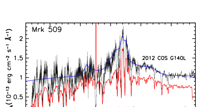
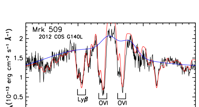
Figure 1: Top panel: Calibrated and merged COS G140L spectrum of Mrk 509 from 2012 (black) compared to the 1999 FUSE spectrum of Kriss et al. (2000) (red). The FUSE spectrum is convolved with the COS line-spread function to render it at the same spectral resolution. The best-fit emission model for the COS G140L is shown in blue. Geocoronal emission at Ly$\beta$ in the FUSE spectrum is indicated with an Earth symbol. Bottom panel: The 2012 COS spectrum, its best-fit emission model, and the 1999 FUSE spectrum are compared in greater detail in the region surrounding the O vi emission line. The FUSE spectrum has been convolved to the COS resolution using the COS line-spread function, and scaled up to match the flux in the red and blue wings of the emission line. Note the higher peak in the emission line for the FUSE spectrum and the subtle differences in the relative strengths of the intrinsic absorption lines.

Table 2: Emission Features in the 2012 COS Spectrum of Mrk 509

Feature	$\rm\lambda_{0}$	Flux	$\rm v_{sys}$	FWHM
	($\rm\AA$)	($\rm 10^{-14}\leavevmode\nobreak\ erg\leavevmode\nobreak\ cm^{-2}\leavevmode\nobreak\ s^{-1}\leavevmode\nobreak\ \AA^{-1}$)	($\rm km\leavevmode\nobreak\ s^{-1}$)	($\rm km\leavevmode\nobreak\ s^{-1}$)
C iii	977.02	$6.1\pm 15.0$	$-10\pm 340$	$1530\pm 260$
C iii	977.02	$25.0\pm 7.2$	$-40\pm 210$	$5580\pm 690$
N iii	989.80	$33.0\pm 32.0$	$270\pm 380$	$8400\pm 670$
Ly$\beta$	1025.72	$170.0\pm 48.0$	$20\pm 370$	$8400\pm 670$
O vi	1031.93	$23.0\pm 4.0$	$610\pm 370$	$1530\pm 260$
O vi	1037.62	$23.0\pm 4.0$	$660\pm 110$	$1530\pm 260$
O vi	1031.93	$30.0\pm 52.0$	$20\pm 360$	$8400\pm 670$
O vi	1037.62	$15.0\pm 26.0$	$20\pm 360$	$8400\pm 670$
Ly$\alpha$	1215.67	$8.9\pm 0.6$	$250\pm 20$	$650\pm 60$
Ly$\alpha$	1215.67	$75.0\pm 2.3$	$-170\pm 20$	$1330\pm 250$
Ly$\alpha$	1215.67	$380.0\pm 12.0$	$-240\pm 20$	$3090\pm 630$
Ly$\alpha$	1215.67	$820.0\pm 25.0$	$-230\pm 20$	$9860\pm 650$
N v	1238.82	$25.0\pm 2.3$	$190\pm 20$	$1920\pm 210$
N v	1242.80	$25.0\pm 2.3$	$180\pm 20$	$1920\pm 210$
S ii	1260.42	$79.0\pm 2.5$	$-10\pm 20$	$6020\pm 200$
O i+S ii	1304.46	$35.0\pm 1.2$	$-70\pm 20$	$3690\pm 190$
C ii	1334.53	$10.0\pm 0.4$	$-10\pm 30$	$2320\pm 230$
Si iv	1393.76	$79.0\pm 2.4$	$40\pm 20$	$4960\pm 190$
Si iv	1402.77	$40.0\pm 1.2$	$40\pm 20$	$4960\pm 190$
N iv]	1486.50	$3.6\pm 41.0$	$-20\pm 50$	$2180\pm 210$
C iv	1548.19	$5.2\pm 1.1$	$-80\pm 40$	$230\pm 30$
C iv	1550.77	$2.6\pm 0.5$	$-80\pm 40$	$230\pm 30$
C iv	1548.19	$82.0\pm 4.1$	$-250\pm 40$	$2040\pm 170$
C iv	1550.77	$41.0\pm 2.0$	$-250\pm 40$	$2040\pm 170$
C iv	1548.19	$200.0\pm 8.5$	$-250\pm 40$	$4270\pm 190$
C iv	1550.77	$99.0\pm 4.3$	$-250\pm 40$	$4270\pm 190$
C iv	1549.48	$440.0\pm 25.0$	$-50\pm 40$	$11480\pm 870$
He ii	1640.45	$8.3\pm 58.0$	$-10\pm 50$	$1200\pm 260$
He ii	1640.45	$71.0\pm 9.2$	$-30\pm 170$	$5040\pm 260$

3 Data Analysis

3.1 Fitting the Continuum and Emission Lines

To compare the intrinsic absorption lines in our 2012 spectra to the prior epochs observed with FUSE and COS, we first fit an emission model to the spectrum in order to produce normalized spectra. As in Kriss et al. (2011), we use a reddened power law to describe the continuum shape and combinations of Gaussian emission components to model the emission lines, with our fits optimized using the specfit task (Kriss, 1994) in IRAF. As in our fits to the 2009 spectrum, we fix the extinction at $\rm E(B-V)=0.057$ (Schlafly & Finkbeiner, 2011) and the foreground damped Ly$\alpha$ absorption by the Milky Way at a column density of $\rm N_{H}=3.9\times 10^{20}\leavevmode\nobreak\ cm^{-2}$ (Wakker et al., 2011). The best-fit power law is very similar to that of the COS 2009 spectrum, with $\rm F_{\lambda}=2.44\times 10^{-13}(\lambda/1000\AA)^{-1.57})$ $\rm erg\leavevmode\nobreak\ cm^{-2}\leavevmode\nobreak\ s^{-1}\leavevmode\nobreak\ \AA^{-1}$.

As in our fits to the 2009 spectrum, we use four Gaussians to describe the strongest lines (Ly$\alpha$, C iv, and O vi)–a very broad base with a full-width at half-maximum of $\sim$10,000 $\rm km\leavevmode\nobreak\ s^{-1}$, two moderate width broad components with FWHM of a few thousand $\rm km\leavevmode\nobreak\ s^{-1}$, and a narrow component with FWHM$\sim$300 $\rm km\leavevmode\nobreak\ s^{-1}$. Weaker lines require only one or two Gaussians. For lines comprised of doublets (O vi, N v, Si iv, and C iv), we include a component for each narrow-line component of the doublet with the relative wavelengths fixed at the ratio of the laboratory values, and an optically thin, 2:1 ratio for the blue to the red flux components. Figure 4 in Kriss et al. (2011) illustrates a similar fit to the 2009 COS spectrum. Table 2 gives the components and best-fit parameters for our model of the 2012 COS spectrum.

Many of the individual components of the spectral features in our fit are significant, but their parameters are highly uncertain. In the case of multi-component lines like C iii $\lambda$977 this is because the Gaussian decomposition we use is not unique. If one takes the feature as a whole, its statistical significance is high, as is the fact that it is not well described by a Gaussian with a single width. In weak lines, one can easily trade flux between components and adjust their widths and positions accordingly. The quoted uncertainties reflect the formal errors associated with this process. Since our overall goal is to determine a total emission model that enables us to normalize the spectrum and measure the depths of the absorption lines, these uncertainties are not an issue.

The best-fit emission model for the COS G140L spectrum is shown overlaying the data in Figure 1. The model smoothly follows the unabsorbed portions of the spectrum. In particular, note that in the regions affected by intrinsic absorption in NGC 5548, the model is quite smooth. Variations in the emission profile are on scales much larger than the absorption troughs. Thus variations in the depths of the troughs that we will discuss later are due to intrinsic variations in the absorption, not variations in the emission model.

3.2 Comparisons to Prior COS and FUSE Spectra

Using the emission model described in the last section, we constructed normalized spectra by dividing the emission model into the deconvolved 2012 COS spectra. We can now directly compare these to the normalized deconvolved COS spectra from 2009. As in Arav et al. (2012), we resampled the G130M and G160M spectra onto a common velocity scale using bins of $5\leavevmode\nobreak\ \rm km\leavevmode\nobreak\ s^{-1}$. Figure 2 compares the Ly$\alpha$, N v, and C iv absorption troughs from these two epochs.

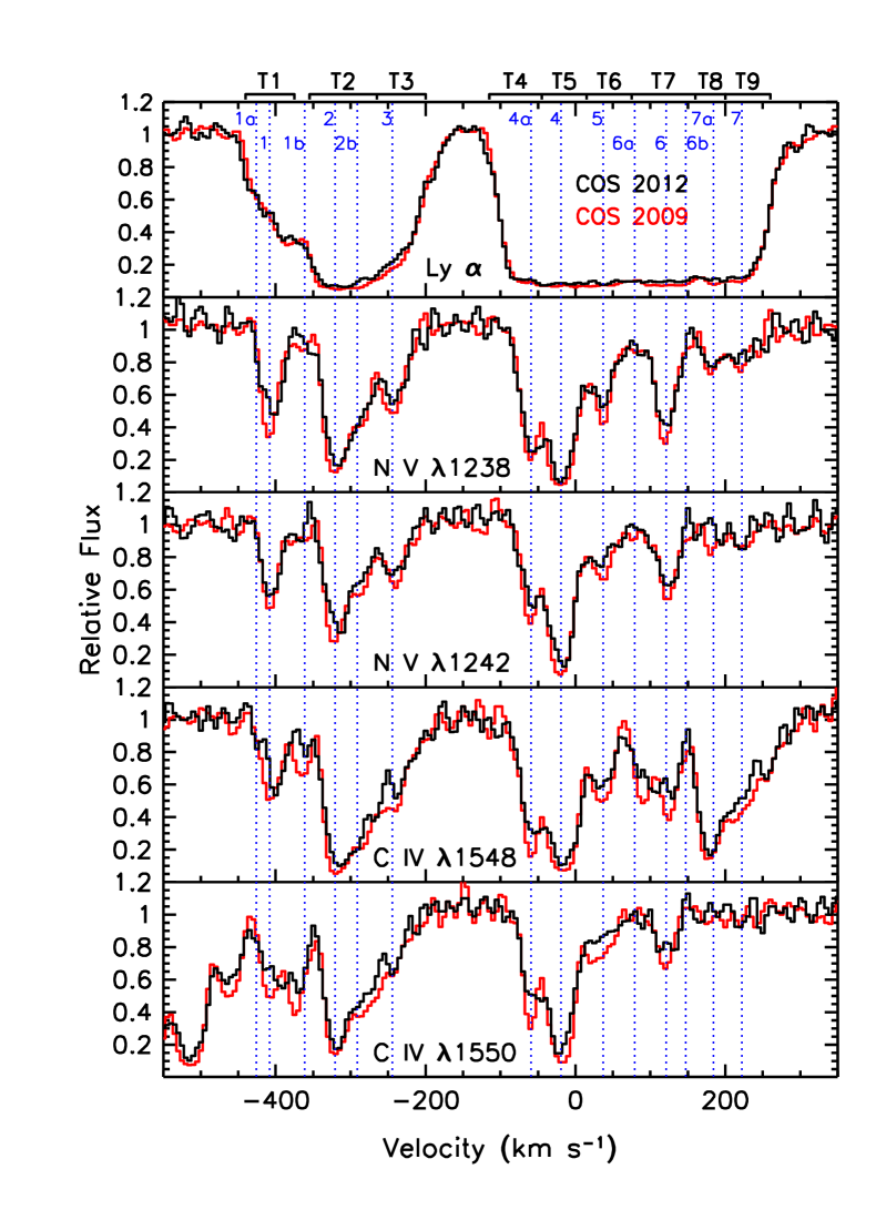
Figure 2: Normalized spectra comparing the intrinsic absorption features in Mrk 509 from COS spectra obtained in 2009 (red) and 2012 (black). Relative fluxes are plotted as a function of velocity relative to the host galaxy redshift of $z=0.034397$ (Fisher et al., 1995). The blue dotted vertical lines are labeled with the components identified by Kriss et al. (2011). The boundaries of the selected spectral regions used to evaluate variability in the absorption troughs are indicated along the top horizontal axis (see also Table 3).

Overall, there are only minor changes in the depths of the intrinsic absorption troughs. To quantitatively evaluate the statistical significance of changes in the absorption troughs, we followed the approach of Arav et al. (2012) to compare the average transmission of the selected spectral regions shown in Figure 2 (labeled T1–T9). Table 3 compares the differences in transmission in each of the absorption troughs T1–T9 between the two epochs. In Ly$\alpha$, the most highly blueshifted troughs, T1 and T2, as well as the main components in the red trough, T4 through T8, show statistically significant variations. The changes are in the sense of increased transmission (decreased absorption) in 2012 compared to 2009. Since Arav et al. (2012) found that the optical depths of the C iv and N v absorption lines in Mrk 509 were not saturated, these variations can be attributed to changes in column density due to photoionization. However, given the high degree of saturation in the Ly$\alpha$ absorption, it is not clear if these might be slight variations in covering factor rather than an ionization response. We therefore do not use Ly$\alpha$ in our analysis below. In N v, as in Arav et al. (2012), to consider a variation to be significant, we require both the red and the blue components to show a consistent change $>2\sigma$ between the COS observations in 2009 and 2012. Under this criterion, we detect significant changes in troughs T1, T3, and T5–T7 in N v. As in Ly$\alpha$, these are all increases in transmission.

Evaluating C iv is more difficult since the close pairing of the doublet transitions ($500\leavevmode\nobreak\ \rm km\leavevmode\nobreak\ s^{-1}$) makes troughs T1–T3 of the red doublet overlap with troughs T7–T9 of the blue doublet. Similarly, trough T7 of the blue doublet is blended with trough T1 of the red doublet. Therefore we can only apply the same criterion of confirmed variability in both red and blue components to troughs T2–T6 for C iv; all of these show increased transmission, as does the single uncontaminated trough T1 in the blue line of the doublet.

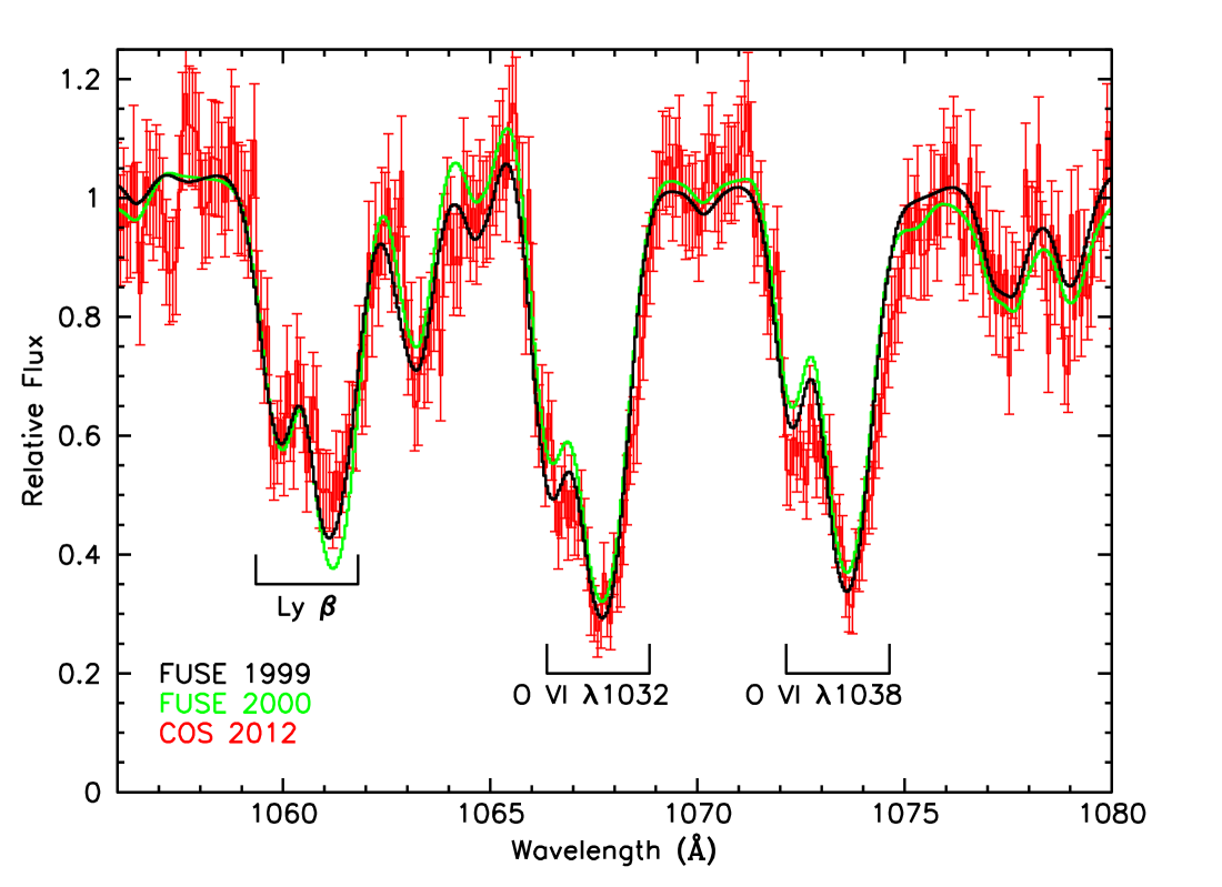
Figure 3: Normalized spectra comparing the intrinsic absorption features in Mrk 509 from the COS G140L spectrum obtained in 2012 (red) to FUSE spectra from 1999 (black) and 2000 (green). 1-$\sigma$ error bars are attached to each COS spectral point. Relative fluxes are plotted as a function of observed wavelength. The Ly$\beta$ and O vi absorption troughs in Mrk 509 are labeled. Other dips in the spectra are foreground galactic interstellar absorption lines.

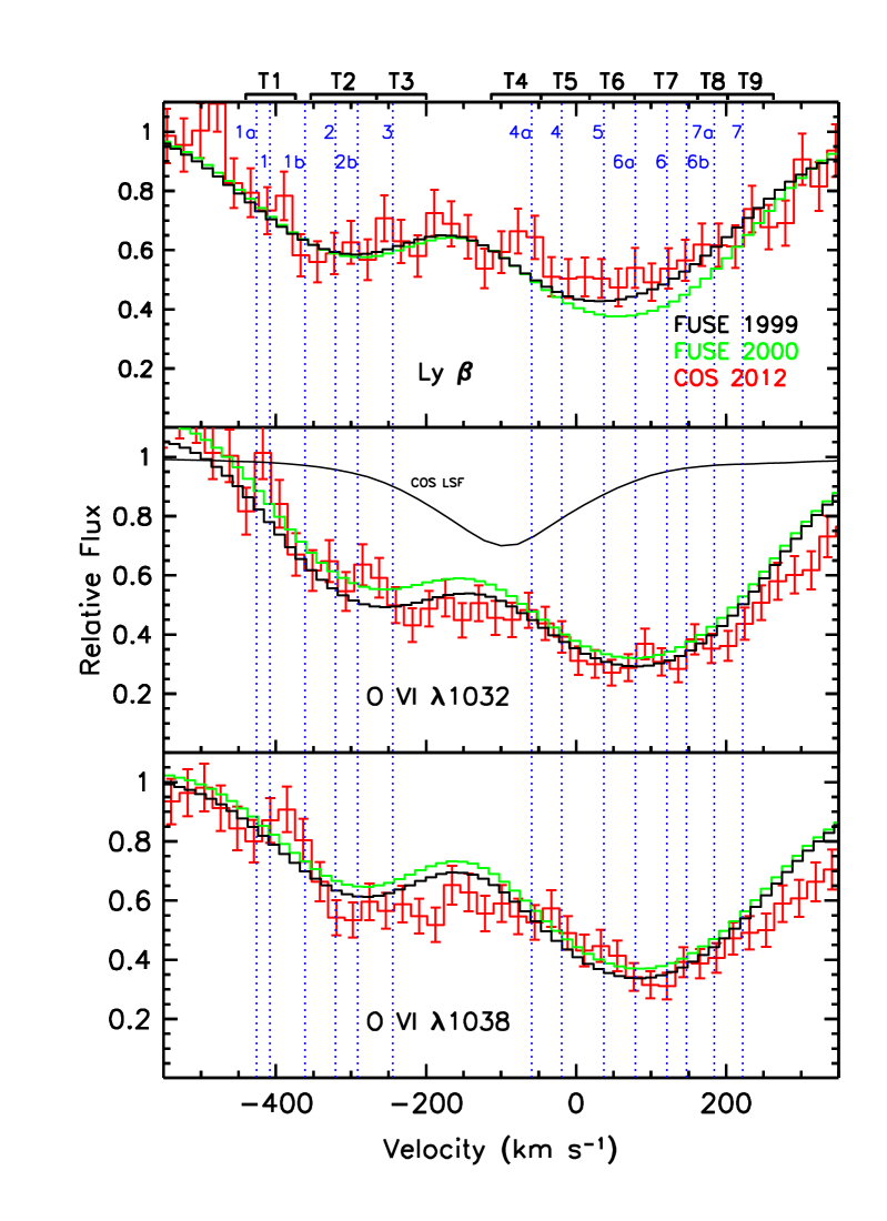
Figure 4: Normalized spectra comparing the intrinsic absorption features in Mrk 509 from the COS G140L spectrum obtained in 2012 (red, with 1-$\sigma$ error bars) to FUSE spectra from 1999 (black) and 2000 (green). Relative fluxes are plotted as a function of velocity relative to the host galaxy redshift of $z=0.034397$ (Fisher et al., 1995). The blue dotted vertical lines are labeled with the components identified by Kriss et al. (2011) at higher spectral resolution. As a guide to the expected widths of unresolved spectral features, the COS line-spread function (LSF) is shown as the thin black line in the middle panel. The boundaries of the selected spectral regions used to evaluate variability in the absorption troughs are indicated along the top horizontal axis (see also Table 5).

These very small variations, although significant, are difficult to evaluate in terms of photoionization models given our extremely sparse sampling. Table 4 summarizes continuum flux measurements at a common wavelength for the prior $\sim$15 years of spectroscopic observations of Mrk 509. Errors on the continuum fluxes in Table 4 are purely statistical. Absolute calibration errors are on the order of 5% for the COS spectra, and 5–10% for FUSE. Arav et al. (2012) found significant variations only in troughs T1 and T2 between the STIS 2001 observation and the COS 2009 observation. While our higher signal-to-noise COS observations from 2012 allow us to detect significant, but very slight changes from 2009, the continuum flux varied hardly at all between the two observations. Given the long response times inferred by Arav et al. (2012) for the outflow in Mrk 509, these slight variations are more reflective of an integrated response to variations over very long timescales, likely years.

Table 3: Variations in Mrk 509 Absorption Troughs between 2009 and 2012

Feature	Absorption	$v_{1}$a	$v_{2}$a	$<T_{COS12}>$b	${<T_{COS12}-T_{COS09}>}^{\mathrm{c}}\over{<T_{COS12}>}$	${\sigma(COS12-COS09)}^{\mathrm{d}}\over{<T_{COS12}>}$	${<T_{COS12}-T_{COS09}>}^{\mathrm{e}}\over{\sigma(COS12-COS09)}$
	Trough	($\rm km\leavevmode\nobreak\ s^{-1}$)	($\rm km\leavevmode\nobreak\ s^{-1}$)
Ly$\alpha$	T1	$-$440	$-$375	0.504	$-$0.001	0.0049	$-$0.1
Ly$\alpha$	T2	$-$355	$-$265	0.106	0.212	0.0096	22.1
Ly$\alpha$	T3	$-$265	$-$200	0.323	0.114	0.0057	19.8
Ly$\alpha$	T4	$-$115	$-$45	0.277	$-$0.013	0.0064	$-$2.1
Ly$\alpha$	T5	$-$45	15	0.082	0.149	0.0126	11.8
Ly$\alpha$	T6	15	75	0.093	0.139	0.0110	12.6
Ly$\alpha$	T7	75	160	0.101	0.175	0.0093	18.8
Ly$\alpha$	T8	160	200	0.113	0.113	0.0128	8.8
Ly$\alpha$	T9	200	260	0.208	0.079	0.0080	9.9
N v $\lambda 1238$	T1	$-$440	$-$375	0.767	0.031	0.0070	4.5
N v $\lambda 1238$	T2	$-$355	$-$265	0.470	0.004	0.0078	0.5
N v $\lambda 1238$	T3	$-$265	$-$200	0.741	0.017	0.0069	2.5
N v $\lambda 1238$	T4	$-$115	$-$45	0.683	$-$0.022	0.0070	$-$3.1
N v $\lambda 1238$	T5	$-$45	15	0.302	0.131	0.0121	10.9
N v $\lambda 1238$	T6	15	75	0.707	0.038	0.0073	5.2
N v $\lambda 1238$	T7	75	160	0.737	0.032	0.0063	5.2
N v $\lambda 1238$	T8	160	200	0.832	$-$0.008	0.0082	$-$0.9
N v $\lambda 1238$	T9	200	260	0.864	$-$0.010	0.0072	$-$1.3
N v $\lambda 1242$	T1	$-$440	$-$375	0.819	0.015	0.0068	2.1
N v $\lambda 1242$	T2	$-$355	$-$265	0.663	0.069	0.0067	10.3
N v $\lambda 1242$	T3	$-$265	$-$200	0.846	0.040	0.0068	5.8
N v $\lambda 1242$	T4	$-$115	$-$45	0.825	0.011	0.0068	1.6
N v $\lambda 1242$	T5	$-$45	15	0.422	0.060	0.0108	5.5
N v $\lambda 1242$	T6	15	75	0.849	0.049	0.0071	6.9
N v $\lambda 1242$	T7	75	160	0.855	0.043	0.0062	6.9
N v $\lambda 1242$	T8	160	200	0.956	0.053	0.0084	6.3
N v $\lambda 1242$	T9	200	260	0.967	0.040	0.0069	5.8
C iv $\lambda 1548$	T1	$-$440	$-$375	0.813	0.059	0.0059	10.0
C iv $\lambda 1548$	T2	$-$355	$-$265	0.365	0.099	0.0079	12.5
C iv $\lambda 1548$	T3	$-$265	$-$200	0.665	0.088	0.0065	13.6
C iv $\lambda 1548$	T4	$-$115	$\phantom{0}-$45	0.682	0.030	0.0061	5.0
C iv $\lambda 1548$	T5	$\phantom{0}-$45	15	0.284	0.058	0.0109	5.4
C iv $\lambda 1548$	T6	15	75	0.716	0.021	0.0063	3.3
C iv $\lambda 1548$	T7	75	160	0.667	0.094	0.0057	16.6
C iv $\lambda 1548$	T8	160	200	0.329	0.106	0.0126	8.5
C iv $\lambda 1548$	T9	200	260	0.576	0.134	0.0075	17.9
C iv $\lambda 1550$	T1	$-$440	$-$375	0.697	0.056	0.0063	8.9
C iv $\lambda 1550$	T2	$-$355	$-$265	0.483	0.119	0.0067	17.7
C iv $\lambda 1550$	T3	$-$265	$-$200	0.813	0.081	0.0059	13.8
C iv $\lambda 1550$	T4	$-$115	$\phantom{0}-$45	0.808	0.020	0.0058	3.5
C iv $\lambda 1550$	T5	$\phantom{0}-$45	15	0.428	0.094	0.0092	10.3
C iv $\lambda 1550$	T6	15	75	0.894	0.067	0.0061	10.9
C iv $\lambda 1550$	T7	75	160	0.928	0.010	0.0052	1.9
C iv $\lambda 1550$	T8	160	200	1.010	0.025	0.0071	3.6
C iv $\lambda 1550$	T9	200	260	0.998	0.008	0.0060	1.4

• Velocities are relative to a systemic redshift of $z=0.034397$ (Fisher et al., 1995).

• Mean transmission in the given absorption trough in the COS 2012 spectrum.

• Mean fractional difference between COS 2012 and COS 2009 troughs normalized by the mean transmission for COS 2012.

• Mean fractional error in the difference between the COS 2012 and COS 2009 troughs normalized by the mean transmission for COS 2012.

• Mean fractional difference between the COS 2012 and COS 2009 troughs normalized by the error.

Table 4: Continuum Fluxes for Mrk 509

Observation	Date	$\rm F_{\lambda}(1160\AA)$
		($\rm 10^{-14}\leavevmode\nobreak\ erg\leavevmode\nobreak\ cm^{-2}\leavevmode\nobreak\ s^{-1}\leavevmode\nobreak\ \AA^{-1}$)
FUSE 1999	1999-11-04	$7.7\pm 0.7$
FUSE 2000	2000-09-05	$4.1\pm 0.2$
STIS 2000	2001-04-13	$5.8\pm 0.2$
COS 2009	2009-12-10	$8.8\pm 0.2$
COS 2012	2012-09-22	$8.8\pm 0.2$

The variations we detected above are consistent with differences seen when we now compare the COS 2012 blue-mode spectra to prior FUSE observations from 1999 and 2000 (Kriss et al., 2000, 2011). Figure 3 compares the normalized COS 2012 G140L spectrum in the Ly$\beta$+O vi region to normalized FUSE spectra from the 1999 and 2000 observations, which have been convolved to the resolution of the COS spectrum.

Significant differences between the COS and FUSE spectra are apparent in the deepest, longer-wavelength portion of the Ly$\beta$ trough, the shallower short wavelength portions of the O vi troughs, and the red wings of the O vi troughs. As with the N v and C iv troughs, we evaluate the statistical significance of any variations by comparing the average transmissions as integrated in the normalized spectra across the troughs labeled T1–T9 in Figure 4. Table 5 summarizes these differences. Although we have used the same velocity bins for this analysis as we did for the high resolution G130M and G160M spectra, we note that the $\sim 150\leavevmode\nobreak\ \rm km\leavevmode\nobreak\ s^{-1}$ resolution of the blue-mode G140L grating really does not resolve troughs T1–T3, or T4–T9. Nevertheless, as shown in Table 5, the aggregate of troughs T4–T8 comprising the heart of the redmost trough in the outflow in Ly$\beta$ all show significantly higher transmission in the COS 2012 spectrum compared to the lower-flux FUSE 2000 observation. In O vi, the blue trough T3 shows significantly decreased transmission in the COS 2012 spectrum compared to FUSE 2000, as do the red troughs T4, T8 and T9. Qualitatively, this is consistent in the sense of a photoionization response since the COS 2012 continuum is more than twice as bright as that in the FUSE 2000 spectrum. The higher flux ionizes more of the neutral hydrogen, increasing the transmission of the Ly$\beta$ trough. This higher ionization state is also consistent with a rise in the ion fraction of O vi for the photoionization models of Kraemer et al. (2003) and Arav et al. (2012).

Table 5: Variations in Mrk 509 Absorption Troughs between 2000 and 2012

Feature	Absorption	$v_{1}$a	$v_{2}$a	$<T_{COS12}>$b	${<T_{COS12}-T_{FUSE00}>}^{\mathrm{c}}\over{<T_{COS12}>}$	${\sigma(COS12-FUSE00)}^{\mathrm{d}}\over{<T_{COS12}>}$	${<T_{COS12}-T_{FUSE00}>}^{\mathrm{e}}\over{\sigma(COS12-FUSE00)}$
	Trough	($\rm km\leavevmode\nobreak\ s^{-1}$)	($\rm km\leavevmode\nobreak\ s^{-1}$)
Ly$\beta$	T1	$-$440	$-$374	0.742	0.033	0.041	0.8
Ly$\beta$	T2	$-$354	$-$266	0.599	0.011	0.038	0.3
Ly$\beta$	T3	$-$266	$-$200	0.624	0.032	0.046	0.7
Ly$\beta$	T4	$-$113	$\phantom{0}-$47	0.621	0.126	0.047	2.7
Ly$\beta$	T5	$\phantom{0}-$48	18	0.532	0.186	0.053	3.5
Ly$\beta$	T6	12	78	0.507	0.243	0.064	3.8
Ly$\beta$	T7	74	162	0.544	0.226	0.045	5.0
Ly$\beta$	T8	158	202	0.610	0.146	0.049	3.0
Ly$\beta$	T9	197	263	0.666	0.018	0.047	0.4
O vi $\lambda 1032$	T1	$-$440	$-$374	0.838	0.003	0.047	0.1
O vi $\lambda 1032$	T2	$-$354	$-$266	0.610	0.009	0.044	0.2
O vi $\lambda 1032$	T3	$-$266	$-$200	0.509	$-$0.104	0.052	$-$2.0
O vi $\lambda 1032$	T4	$-$113	$-$47	0.454	$-$0.123	0.048	$-$2.6
O vi $\lambda 1032$	T5	$\phantom{0}-$48	18	0.375	$-$0.075	0.052	$-$1.4
O vi $\lambda 1032$	T6	12	78	0.291	$-$0.157	0.064	$-$2.5
O vi $\lambda 1032$	T7	74	162	0.330	$-$0.050	0.058	$-$0.9
O vi $\lambda 1032$	T8	158	202	0.366	$-$0.170	0.079	$-$2.2
O vi $\lambda 1032$	T9	197	263	0.457	$-$0.209	0.049	$-$4.3
O vi $\lambda 1038$	T1	$-$440	$-$374	0.851	0.022	0.031	0.7
O vi $\lambda 1038$	T2	$-$354	$-$266	0.610	$-$0.101	0.036	$-$2.8
O vi $\lambda 1038$	T3	$-$266	$-$200	0.569	$-$0.192	0.043	$-$4.5
O vi $\lambda 1038$	T4	$-$113	$\phantom{0}-$47	0.552	$-$0.132	0.044	$-$3.0
O vi $\lambda 1038$	T5	$\phantom{0}-$48	18	0.498	0.033	0.047	0.7
O vi $\lambda 1038$	T6	12	78	0.407	0.034	0.061	0.5
O vi $\lambda 1038$	T7	74	162	0.350	$-$0.119	0.054	$-$2.2
O vi $\lambda 1038$	T8	158	202	0.414	$-$0.129	0.054	$-$2.4
O vi $\lambda 1038$	T9	197	263	0.478	$-$0.211	0.046	$-$4.5

• Velocities are relative to a systemic redshift of $z=0.034397$ (Fisher et al., 1995).

• Mean transmission in the given absorption trough in the COS 2012 spectrum.

• Mean fractional difference between COS 2012 and FUSE 2000 troughs normalized by the mean transmission for COS 2012.

• Mean fractional error in the difference between the COS 2012 and FUSE 2000 troughs normalized by the mean transmission for COS 2012.

• Mean fractional difference between the COS 2012 and FUSE 2000 troughs normalized by the error.

Since we detect variations in the transmission of all absorption troughs in Mrk 509 in our most recent COS observation, we can use the timescale of these variations to set lower limits on the density of each of the absorption components based on the recombination timescale (Krolik & Kriss, 1995; Nicastro et al., 1999; Arav et al., 2012). Given the slight variations we observe in column density, we use the same baseline photoionization solutions for each absorption trough as Arav et al. (2012), and use the associated timescales per electron number density for these solutions for C iv and N v as given in their Table 6. For troughs 8 and 9 in O vi, we use the photoionization solution of Kraemer et al. (2002), and obtain the timescale per electron number density for O vi from the Cloudy output (Ferland et al., 2017).

For our sparsely sampled data, the fractional variation in the continuum between our two widely spaced observations in 2009 and 2012 is unknown. The actually observed variation is only 0.6%, but it is possible that Mrk 509 dropped in flux by 100% immediately after the COS 2009 observation, and then recovered to normal fluxes by 2012. We therefore use this conservative assumption. Since the gas density must be high enough to respond to such variations at least on the timescale corresponding to the interval between our two observations, we can set a lower limit on the density, which then translates into an upper limit on the distance.

In Table 6 we give upper limits on the density as determined by Arav et al. (2012) from the lack of variations observed between 2001 and 2009 for both C iv and N v, and lower limits on the density as determined from the variations we observed between 2009 and 2012. These both translate into lower and upper limits on the distance of the absorbing gas from the nucleus. For the lower limits, we use the 99% confidence limits given in Table 8 of Arav et al. (2012). For the upper limits, we use the most stringent (smallest) distance implied by our lower limits on the density determined by either the C iv, N v, or O vi measurements. Although the bounds on radial distance given in the last two columns of Table 6 appear to locate the absorbing gas quite precisely, our sparse sampling in time and many assumptions suggest great caution in jumping to this conclusion. In particular, we note that for some components, e.g., T3, T6, and T7, our upper and lower bounds on density and distance are incommensurate. We attribute this to the statistical nature of our analysis and the sparse sampling. The lower limits on distance derived from the Monte Carlo simulations in Arav et al. (2012) are based mostly on the lack of variations detected between the STIS observations and the COS observations. Not observing variations is a function of both the actual strength of the change in absorption as well as having observations sufficiently sensitive to detect variations. The STIS 2001 observation has significantly less signal-to-noise than either COS observation; more sensitive observations in 2001 may well have led to detection of variations at the level we observed between 2009 and 2012. Given these uncertainties, it is quite likely that the lower limits on distance can easily be much lower than the 99% confidence limits of Arav et al. (2012).

Table 6: Limits on Density and Distance for Mrk 509 Absorption Troughs

		C iv		N v		O vi
Trough	Velocity	$n_{e,low}^{\rm a}$	$n_{e,high}$	$n_{e,low}^{\rm a}$	$n_{e,high}$	$n_{e,low}$	$n_{e,high}$	$R_{low}^{\rm b}$	$R_{high}^{\rm c}$
	($\rm km\leavevmode\nobreak\ s^{-1}$)	($\rm log\leavevmode\nobreak\ cm^{-3}$)	($\rm log\leavevmode\nobreak\ cm^{-3}$)	($\rm log\leavevmode\nobreak\ cm^{-3}$)	($\rm log\leavevmode\nobreak\ cm^{-3}$)	($\rm log\leavevmode\nobreak\ cm^{-3}$)	($\rm log\leavevmode\nobreak\ cm^{-3}$)	(pc)	(pc)
(1)	(2)	(3)	(4)	(5)	(6)	(7)	(8)	(9)	(10)
T1	$-408$	$\;\stackrel{{\scriptstyle>}}{{\sim}}\;$3.3	…	$\;\stackrel{{\scriptstyle>}}{{\sim}}\;$2.8	$\;\stackrel{{\scriptstyle<}}{{\sim}}\;$4.2	…	…	$\;\stackrel{{\scriptstyle>}}{{\sim}}\;$  60	$\;\stackrel{{\scriptstyle<}}{{\sim}}\;$130
T2	$-310$	$\;\stackrel{{\scriptstyle>}}{{\sim}}\;$3.0	$\;\stackrel{{\scriptstyle<}}{{\sim}}\;$3.2	…	$\;\stackrel{{\scriptstyle<}}{{\sim}}\;$4.2	…	…	$\;\stackrel{{\scriptstyle>}}{{\sim}}\;$160	$\;\stackrel{{\scriptstyle<}}{{\sim}}\;$170
T3	$-233$	$\;\stackrel{{\scriptstyle>}}{{\sim}}\;$2.6	$\;\stackrel{{\scriptstyle<}}{{\sim}}\;$3.2	$\;\stackrel{{\scriptstyle>}}{{\sim}}\;$2.6	$\;\stackrel{{\scriptstyle<}}{{\sim}}\;$3.9	$\;\stackrel{{\scriptstyle>}}{{\sim}}\;$1.6	…	$\;\stackrel{{\scriptstyle>}}{{\sim}}\;$130	$\;\stackrel{{\scriptstyle<}}{{\sim}}\;$130
T4	$-80$	$\;\stackrel{{\scriptstyle>}}{{\sim}}\;$2.5	$\;\stackrel{{\scriptstyle<}}{{\sim}}\;$3.1	…	$\;\stackrel{{\scriptstyle<}}{{\sim}}\;$3.4	$\;\stackrel{{\scriptstyle>}}{{\sim}}\;$1.6	…	$\;\stackrel{{\scriptstyle>}}{{\sim}}\;$130	$\;\stackrel{{\scriptstyle<}}{{\sim}}\;$220
T5	$-15$	$\;\stackrel{{\scriptstyle>}}{{\sim}}\;$2.5	$\;\stackrel{{\scriptstyle<}}{{\sim}}\;$3.6	$\;\stackrel{{\scriptstyle>}}{{\sim}}\;$2.8	…	…	…	$\;\stackrel{{\scriptstyle>}}{{\sim}}\;$130	$\;\stackrel{{\scriptstyle<}}{{\sim}}\;$220
T6	$+45$	$\;\stackrel{{\scriptstyle>}}{{\sim}}\;$2.3	$\;\stackrel{{\scriptstyle<}}{{\sim}}\;$2.8	$\;\stackrel{{\scriptstyle>}}{{\sim}}\;$3.1	$\;\stackrel{{\scriptstyle<}}{{\sim}}\;$3.1	…	…	$\;\stackrel{{\scriptstyle>}}{{\sim}}\;$150	$\;\stackrel{{\scriptstyle<}}{{\sim}}\;$  90
T7	$+118$	…	$\;\stackrel{{\scriptstyle<}}{{\sim}}\;$2.5	$\;\stackrel{{\scriptstyle>}}{{\sim}}\;$2,4	…	…	…	$\;\stackrel{{\scriptstyle>}}{{\sim}}\;$130	$\;\stackrel{{\scriptstyle<}}{{\sim}}\;$120
T8	$+180$	$\;\stackrel{{\scriptstyle>}}{{\sim}}\;$1.8	…	…	…	$\;\stackrel{{\scriptstyle>}}{{\sim}}\;$2.3	…	…	$\;\stackrel{{\scriptstyle<}}{{\sim}}\;$140
T9	$+230$	…	…	…	…	$\;\stackrel{{\scriptstyle>}}{{\sim}}\;$2.3	…	…	$\;\stackrel{{\scriptstyle<}}{{\sim}}\;$140

• Column (1): Absorption trough as defined in Table 4. Column (2): Central velocity of the trough ($\rm km\leavevmode\nobreak\ s^{-1})$. Column (3): Lower limit on the density derived from C iv ($\rm log\leavevmode\nobreak\ cm^{-3}$). Column (4): Upper limit on the density derived from C iv ($\rm log\leavevmode\nobreak\ cm^{-3}$). Column (5): Lower limit on the density derived from N v ($\rm log\leavevmode\nobreak\ cm^{-3}$). Column (6): Upper limit on the density derived from N v ($\rm log\leavevmode\nobreak\ cm^{-3}$). Column (7): Lower limit on the density derived from O vi ($\rm log\leavevmode\nobreak\ cm^{-3}$). Column (8): Upper limit on the density derived from O vi ($\rm log\leavevmode\nobreak\ cm^{-3}$). Column (9): Lower limit on the distance (pc). Column (10): Upper limit on the distance (pc).
  ^a Upper limits on density taken from Table 8 of Arav et al. (2012).
  ^b Lower limits on distance taken from the 99% confidence limits in Table 8 of Arav et al. (2012).
  ^c Upper limits on distance use the most stringent (highest) limits on the density from either C iv, N v, or O vi.

3.3 No Features Related to Ultra-fast Outflows

Mrk 509 is among the growing number of AGN in which ultra-fast outflows (UFO) have been detected in X-ray observations (Tombesi et al., 2010; Gofford et al., 2013). These outflows typically have velocities exceeding 10,000 $\rm km\leavevmode\nobreak\ s^{-1}$ and high column densities $(>10^{23}\leavevmode\nobreak\ \rm cm^{-2})$. Due to their high ionization, they often only show absorption in Fe xxv or Fe xxvi. Despite their high ionization, it is possible for X-ray UFOs to show related absorption in H i Ly$\alpha$ due to the high total column density of the UFO, as seen in the quasar PG1211+143 (Danehkar et al., 2018). As with the X-ray absorption features, these UV counterparts are also variable (Kriss et al., 2018b).

In Mrk 509, Tombesi et al. (2010) reported three systems with $v_{out}=-0.141c,-0.172c,\mathrm{and}-0.196c$. Ponti et al. (2009) reported yet a fourth system at $v_{out}=-0.141c$ in the stacked XMM-Newton spectra. In the 2009 XMM-Newton campaign on Mrk 509, no UFO features were seen (Ponti et al., 2013). Similarly, in the Chandra observations coordinated with these HST observations, UFOs were also not detected. Kriss et al. (2018a) searched for Ly$\alpha$ counterparts to these X-ray UFOs in the archival FUSE observations of Mrk 509 and found none.

Given the strong variability of UFOs, we have searched our new HST spectra for possible counterparts. The lower resolution of the COS G140L grating compared to FUSE makes this more difficult due to the unresolved absorption from many interstellar absorption lines. However, when we compare our G140L spectrum to the FUSE spectra convolved with the G140L line-spread function and scaled to the G140L flux levels, we find no differences. We therefore set upper limits for Ly$\alpha$ counterparts to the previously detected X-ray UFOs at the same levels as reported in Kriss et al. (2018a). For the three features at $v_{out}=-0.141c,-0.172c,\mathrm{and}-0.196c$, we set $2\sigma$ confidence level (95%) upper limits on the H i column density of $\mathrm{N_{H}}<1.1\times 10^{13}\leavevmode\nobreak\ \mathrm{cm}^{-2},7.2\times 10^{12}\leavevmode\nobreak\ \mathrm{cm}^{-2},\leavevmode\nobreak\ \mathrm{and}\leavevmode\nobreak\ 1.3\times 10^{14}\leavevmode\nobreak\ \mathrm{cm}^{-2}$, respectively. The feature at $v_{out}=-0.048c$ falls at 1197 Å, within the bandpass of our high-resolution, high S/N G130M spectra. No absorption is found beyond the usual narrow interstellar features of Mn ii $\lambda\lambda 1197,1199$ and the N i triplet at 1200 Å. For a broad absorption feature with FWHM=1000 $\rm km\leavevmode\nobreak\ s^{-1}$, we set an upper limit on the equivalent width of 0.05 Å, and an upper limit on the H i column density of $9.2\times 10^{12}\leavevmode\nobreak\ \mathrm{cm}^{-2}$.

4 Discussion

Our HST/COS observations of Mrk 509 in 2012 supplement the extensive multiwavelength campaign carried out with XMM-Newton, Chandra, and HST in 2009 (Kaastra et al., 2011). These new FUV spectra sample variations in the intrinsic UV absorption troughs on both shorter timescales ($\sim$3 years) and longer ones ($\sim 13$ years) than our original campaign. The shorter timescale variations permit us to put better upper limits on the location of the outflowing gas than was possible in Kriss et al. (2011) and Arav et al. (2012).

Kriss et al. (2011) detected variations in absorption Component #6 of Ly$\beta$, which allowed them to set an upper limit of 1.25 kpc on its distance. This absorption component comprises the bulk of trough T7 in Arav et al. (2012). The lack of variability in this trough in both N v and C iv between the STIS 2001 observation and the COS 2009 spectrum led to a lower limit on its distance of $>130$ pc at the 99% confidence level, consistent with the 1.25 kpc upper limit from Ly$\beta$ variability. However, our new COS observations in 2012 do detect variability in trough T7 on shorter timescales than those sampled between the STIS 2001 and COS 2009 observations. This illustrates the difficulty of drawing firm conclusions based on poorly sampled data. Lack of variability does not always imply a firm upper limit on the gas density. It can be simply by chance that sparse observations observe the same transmission, even though the absorption troughs are varying on more rapid timescales. In the case of trough T7, the change we see in the 3 years between the two COS observations imply a minimum density of log $n_{e}\leavevmode\nobreak\ \rm cm^{-3}>2.4$ and a corresponding upper limit on its distance of 120 pc, comparable to the upper limit based on non-detection. Our new COS G140L blue-mode observations of the Ly$\beta$+O vi region confirm variability at these velocities in trough T7 (which includes Component #6), but on the longer timescale of 12 years, compared to 2 years. This Ly$\beta$ variability does not improve our upper limit on the distance, but it does confirm the detection of the column density variation we see in N v.

The outflow as manifested in the UV absorption lines is centrally concentrated in the near nuclear region. All absorption troughs have distances within $<$220 pc of the nucleus. At the redshift of Mrk 509 ($z=0.03937$), a Hubble constant of $H_{o}=70\leavevmode\nobreak\ \rm km\leavevmode\nobreak\ s^{-}1\leavevmode\nobreak\ Mpc^{-1}$, $\Omega_{DM}=0.3$, and $\Omega_{\Lambda}=0.7$, in the rest frame of the cosmic microwave background, the angular scale at the distance of Mrk 509 is 667 $\rm pc\leavevmode\nobreak\ arcsec^{-1}$. This places the troughs at angular scales of $<0.3^{\prime\prime}$, which corresponds to the unresolved, highest surface brightness central peak in the optical and near-IR IFU observations of Mrk 509 (Fischer et al., 2015; Liu et al., 2015). Given that this region is unresolved, the UV absorption troughs could correspond to filaments observed at similar distances in nearby AGN such as NGC 4151 (Das et al., 2005) or NGC 1068 (Das et al., 2007). As suggested by Crenshaw & Kraemer (2012), the kinematics, ionization state, and densities of these high-excitation emission-line knots and filaments are very similar to the physical characteristics of the narrow UV absorption lines observed in most low-redshift AGN.

The high blue-shifted velocities of troughs T1–T3 do not correspond to typical velocities observed in the IFU images, which range $\sim-250$–$+250\leavevmode\nobreak\ \rm km\leavevmode\nobreak\ s^{-1}$ (Fischer et al., 2015; Liu et al., 2015), nor do they lie at the highest distances (up to $\sim$1.5 kpc) seen in the IFU images. The lower velocities at larger distances observed in the IFU images resemble the behavior seen in the resolved structures near the centers of NGC 4151 and NGC 1068. The inner clouds have increasing velocity with distance until reaching a maximum at $\sim$100 pc. At larger distances, velocities decrease. This might suggest that the outflowing gas becomes mass loaded as it entrains surrounding material from the ambient ISM, and then decelerates (Das et al., 2005, 2007). If similar mechanisms are at work in Mrk 509, the overall impact on the host galaxy is small. Liu et al. (2015) note that a small region northeast of the nucleus in Mrk 509 appears to have suppressed star formation, perhaps due to the impact of the AGN outflow. However, there are many other star-forming regions at larger radii that appear normal. So, the visible impact of the AGN outflow on the overall character of the host galaxy appears to be minimal.

5 Conclusions

Sensitive HST/COS observations of Mrk 509 in 2012 following the multiwavelength campaign of Kaastra et al. (2011) allow us to detect variations in absorption in the AGN outflow when compared to prior UV spectral observations. We detect significant changes on a shorter 3-year timescale that allow us to set upper limits on the distance of most absorption troughs at distances of 100–200 pc. This is consistent with the location established for the X-ray warm absorbers (5–400 pc) by Kaastra et al. (2012). It also corresponds to the unresolved central peak in IFU observations of the narrow-line region of Mrk 509. The nuclear outflow appears to have most of its impact confined to the near-nuclear region, and have little impact on the host galaxy overall.