Preface

These notes have been prepared for a series of lectures given at the Sarajevo Stochastic Analysis Winter School, from January 28 to February 1, 2019. There already exist several excellent lecture notes and reviews on the subject, such as [Hairer_LN_2009] on (non-singular) stochastic PDEs, and [Hairer_LN_2015, Chandra_Weber_LN17] on singular stochastic PDEs and regularity structures. The present notes have two main specificities. The first one is that they focus on a particular example, the Allen–Cahn equation, which allows to introduce several of the difficulties of the theory in a gradual way, by increasing the space dimension step by step. The hope is that while this limits the generality of the theory presented, this limitation is more that made up by a gain in clarity. The second specific aspect of these notes is that they go beyond existence and uniqueness of solutions, by covering a few recent results on convergence to equilibrium and metastability in these system.

The author wishes to thank the organisers of the Winter School, Frank Proske, Abdol-Reza Mansouri and Oussama Amine, for the invitation that provided the motivation to compile these notes; his co-workers on SPDEs, Ajay Chandra, Giacomo Di Gesù, Barbara Gentz, Christian Kuehn and Hendrik Weber, who greatly contributed to some results presented here; Yvain Bruned for remarks on an early version of the notes; and Martin Hairer and Lorenzo Zambotti for patiently explaining some subtleties of the theory of regularity structures.

Thanks are also due to the Isaac Newton Institute in Cambridge, as well as David Brydges, Alessandro Giuliani, Massimiliano Gubinelli, Antti Kupiainen, Hendrik Weber and Lorenzo Zambotti for organising the semester “Scaling limits, rough paths, quantum field theory”. In particular the tutorial lectures given during the opening workshop of the semester proved of great help in preparing these notes.

Finally, thanks are due to Adrian Martini, for pointing out some typos in the original version of these notes.

Chapter 1 A system of interacting diffusions

In this chapter, we will analyse the dynamics of a system of $N\mathbin{\geqslant}2$ coupled stochastic differential equations (SDEs), which will converge, in a certain sense, to a stochastic Allen–Cahn PDE. This will serve two purposes: firstly, it will introduce a natural physical model that motivates the use of stochastic PDEs, and secondly, it will allow us to recapitulate some notions from the theory of SDEs that will be important in the infinite-dimensional case.

The system of interacting diffusions is given by

$$\operatorname{d}\!y^{i}_{t}=\bigl{[}y^{i}_{t}-(y^{i}_{t})^{3}\bigr{]}\operatorname{d}\!t+\frac{\gamma}{2}\bigl{[}y^{i+1}_{t}-2y^{i}_{t}+y^{i-1}_{t}\bigr{]}\operatorname{d}\!t+\sqrt{2\varepsilon}\operatorname{d}\!W^{i}_{t}\;,\qquad i=1,\dots,N\;,$$ (1.0.1)

in the following setting.

• The real variables $y^{1},\dots,y^{N}\in\mathbb{R}$ can be thought of as the positions of $N$ particles. We use periodic boundary conditions, that is, $y^{0}=y^{N}$ and $y^{N+1}=y^{1}$. This can also be indicated by considering $i$ as an element of the cyclic group $\Lambda=\mathbb{Z}/N\mathbb{Z}$.

• The term $[y^{i}_{t}-(y^{i}_{t})^{3}]\operatorname{d}\!t$ tends to push each particle towards $+1$ if $y^{i}_{t}>0$ and towards $-1$ if $y^{i}_{t}<0$, that is, we have a bistable local dynamics.

• The term $\smash{\frac{\gamma}{2}}[y^{i+1}_{t}-2y^{i}_{t}+y^{i-1}_{t}]\operatorname{d}\!t$ is a discretised Laplacian interaction, which describes a ferromagnetic nearest-neighbour coupling pushing the $y^{i}_{t}$ towards each other (if $\gamma>0$).

• The $W^{i}_{t}$ are independent standard Wiener processes on a probability space $(\Omega,{\mathscr{F}},\mathbb{P})$, modelling thermal noise.

The system (1.0.1) can be thought of as a version of the Ising model with continuous spins. We are mainly interested in its long-time dynamics for large values of $N$ and $\gamma$. The parameter $\varepsilon\mathbin{\geqslant}0$ will be either small or of order $1$.

1.1 Deterministic dynamics

In the deterministic case $\varepsilon=0$, the system (1.0.1) reduces to the system of ordinary differential equations (ODEs)

$$\dot{y}^{i}=y^{i}-(y^{i})^{3}+\frac{\gamma}{2}\bigl{[}y^{i+1}-2y^{i}+y^{i-1}\bigr{]}\;.$$ (1.1.1)

A first observation is that (1.1.1) has gradient form

$$\dot{y}=-\nabla V(y)\;,$$ (1.1.2)

where $V$ is the quartic potential given by

$$V(y):=\sum_{i\in\Lambda}U(y^{i})+\frac{\gamma}{4}\sum_{i\in\Lambda}(y^{i+1}-y^{i})^{2}\;,\qquad U(\xi)=\frac{1}{4}\bigl{(}\xi^{2}-1\bigr{)}^{2}\;.$$ (1.1.3)

The stationary points of (1.1.1) are thus the critical points of $V$. Note that $V$ is invariant under the group $G$ generated by cyclic permutations of the $y^{i}$, the reflection $y^{i}\mapsto y^{N+1-i}$, and the point symmetry $y\mapsto-y$.

The simplest situation arises for $\gamma=0$: then the set of all critical points of $V$ is $\{-1,0,1\}^{\Lambda}$ and has cardinality $3^{N}$. The critical points in $\{-1,1\}^{\Lambda}$ are all local minima of $V$, and thus describe $2^{N}$ stable stationary points of (1.1.1). In fact, one can show [BFG06a, Proposition 2.1] that this situation perturbs to small positive $\gamma$, in the sense that there are still $3^{N}$ stationary points, $2^{N}$ of which are stable, for all $\gamma$ up to a critical value $\gamma_{0}(N)$ which is larger than $\frac{1}{4}$ for all $N$.

We are more interested, however, in the case of large $\gamma$ of the order $N^{2}$. Indeed, this is the natural scaling in which the discrete Laplacian in (1.1.1) approaches the continuous Laplacian.

Proposition 1.1.1.

Let

$$\gamma_{1}(N):=\frac{1}{2\sin^{2}(\pi/N)}=\frac{N^{2}}{2\pi^{2}}\Bigl{[}1+{\mathcal{O}}\Bigl{(}\frac{1}{N^{2}}\Bigr{)}\Bigr{]}\;.$$ (1.1.4)

Then the potential $V$ admits exactly $3$ stationary points $0$ and $\pm(1,\dots,1)$ if and only if $\gamma\mathbin{\geqslant}\gamma_{1}(N)$. The points $\pm(1,\dots,1)$ are always local minima of $V$, while $0$ is a saddle with exactly one linearly unstable direction if and only if $\gamma>\gamma_{1}(N)$.

Proof:.

First note that the discrete Laplacian is represented by a Toeplitz matrix (its entries are constant on diagonals), whose eigenvalues can be computed explicitly by discrete Fourier transform. They are given by $-\lambda^{N}_{k}$ where

$$\lambda^{N}_{k}=\lambda^{N}_{N-k}:=2\sin^{2}\biggl{(}\frac{k\pi}{N}\biggr{)}\;,\qquad k=0,\dots,N-1\;.$$ (1.1.5)

In particular, $\lambda^{N}_{0}=0$ and $\gamma_{1}(N)=1/(\lambda^{N}_{1}-\lambda^{N}_{0})$ is the inverse of the spectral gap. Consider now the function

$$W(y):=\frac{1}{2}\sum_{i\in\Lambda}\bigl{(}y^{i+1}-y^{i}\bigr{)}^{2}\;.$$ (1.1.6)

Note that $W$ vanishes on the diagonal $\{y^{1}=\dots=y^{N}\}$ and is otherwise positive. An easy computation (cf. [BFG06a, Proposition 3.1]) shows that

$$\frac{\operatorname{d}\!}{\operatorname{d}\!t}W(y_{t})\mathbin{\leqslant}2\Bigl{(}1-\frac{\gamma}{\gamma_{1}(N)}\Bigr{)}W(y_{t})-\frac{1}{N}W(y_{t})^{2}\;.$$ (1.1.7)

Thus when $\gamma\mathbin{\geqslant}\gamma_{1}(N)$, $t\mapsto W(y_{t})$ decreases for $y_{t}$ outside the diagonal, i.e., $W$ is a Lyapunov function. Therefore, when $\gamma\mathbin{\geqslant}\gamma_{1}(N)$ all orbits of (1.1.1) will converge to the diagonal. The only stationary points on the diagonal are $0$ and $\pm(1,\dots,1)$. The eigenvalues of the linearisation of (1.1.1) at $0$ are given by $-\mu^{N}_{k}$ where

$$\mu^{N}_{k}:=-1+\gamma\lambda^{N}_{k}\;,\qquad k=0,\dots,N-1\;.$$ (1.1.8)

If $\gamma>\gamma_{1}(N)$, then only $-\mu^{N}_{0}$ is positive, while for $\gamma<\gamma_{1}(N)$, there are at least three positive eigenvalues (two if $N=2$). Since $V(y)$ is bounded below and goes to infinity as $\lVert y\rVert\to\infty$, there must be critical points outside the diagonal in the latter case. Finally, the eigenvalues of the linearisation at $\pm(1,\dots,1)$ are given by $-\nu^{N}_{k}$ where

$$\nu^{N}_{k}:=2+\gamma\lambda^{N}_{k}\;,\qquad k=0,\dots,N-1\;.$$ (1.1.9)

These are always negative, showing that these points are always stable (they are local minima of $V$). ∎

Exercise 1.1.2.

Show that the potential satisfies the lower bound

$$V(y_{0}+y_{\perp})\mathbin{\geqslant}V(y_{0})+\frac{1}{2}\Bigl{(}\frac{\gamma}{\gamma_{1}(N)}-1\Bigr{)}\,\lVert y_{\perp}\rVert^{2}$$ (1.1.10)

whenever $y_{0}$ belongs to the diagonal $\{y^{1}=\dots=y^{N}\}$ and $y_{\perp}$ is orthogonal to the diagonal.

This result shows that if $\gamma>\gamma_{1}(N)$, then $V$ is a double-well potential, with a saddle having one unstable direction located at the origin, and the two minima located at $\pm(1,\dots,1)$. The unstable manifolds of the saddle are subsets of the diagonal, and connect $0$ to the two local minima. This is the case we will mainly be interested in in what follows.

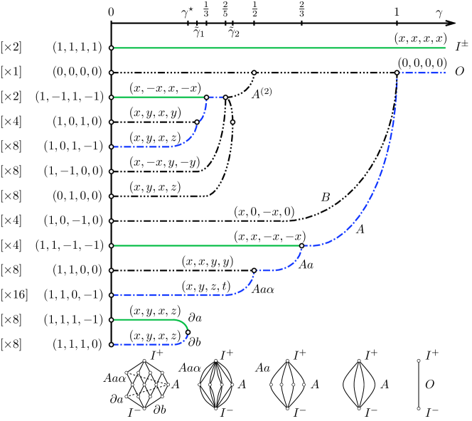
Figure 1.1: Schematic bifurcation diagram for (1.1.1) in the case $N=4$. Each branch in this diagram represents a family of stationary points globally invariant under the symmetry group $G$, with only one representative of the family displayed on the left side of the diagram. Green full lines represent stable stationary points (local minima of the potential $V$), while broken lines with $k$ dots represent stationary points with $k$ unstable directions (saddles of Morse index $k$ of $V$).

As $\gamma$ decreases below $\gamma_{1}(N)$, the situation becomes much more involved, and is not understood in full detail. What is known is that at $\gamma_{1}(N)$, the system undergoes a $G$-symmetric analogue of a pitchfork bifurcation, at which the origin becomes unstable in more than one direction, while expelling a multiple of $N$ new stationary points with lower symmetry. As $\gamma$ decreases further, these points undergo further symmetry-breaking bifurcations, as illustrated by Figure 1.1 in the case $N=4$. However, all these further bifurcation occur for $\gamma={\scriptstyle\mathcal{O}}(N^{2})$. In other words, for any $\tilde{\gamma}>0$, the number of stationary points is at most of order $N$ when $\gamma>\tilde{\gamma}N^{2}$ and $N$ is sufficiently large.

Exercise 1.1.3.

In the case $N=2$, find all stationary points of the potential $V$ and determine their stability as a function of $\gamma\mathbin{\geqslant}0$. Hint: Express the potential $V$ in variables $z_{\pm}=y_{1}\pm y_{2}$.

1.2 Existence and uniqueness of solutions

We now return to the SDE (1.0.1) for $\varepsilon>0$. We can write it in compact form as

$$\operatorname{d}\!y_{t}=-\nabla V(y_{t})\operatorname{d}\!t+\sqrt{2\varepsilon}\operatorname{d}\!W_{t}\;.$$ (1.2.1)

We first note that $y\mapsto\nabla V(y)$ is continuous (and therefore measurable) and locally (but not globally) Lipschitz. We can thus apply a standard result, such as [Oeksendal, Theorem 5.2.1] to the process $y_{t\wedge\tau}$ where $\tau$ is the first-exit time from a large ball to obtain local existence and uniqueness of a strong solution to (1.2.1). In particular, local existence follows from the fact that the map $y^{(k)}\mapsto y^{(k+1)}$ defined by

$$y_{t}^{(k+1)}=y_{0}-\int_{0}^{t\wedge\tau}\nabla V(y^{(k)}_{s})\operatorname{d}\!t+\sqrt{2\varepsilon}W_{t}$$ (1.2.2)

is a contraction, via Banach’s fixed point theorem.

To extend this result to global existence of a strong solution, we have to rule out finite-time explosion of solutions. This is, however, not hard to achieve, since the quartic growth of the potential prevents sample paths from straying very far from the origin (coercivity). Here are two possible ways of obtaining global existence:

1. One checks that the drift and diffusion coefficients in (1.2.1) satisfy the one-sided growth condition

   $$y\cdot\bigl{(}-\nabla V(y)\bigr{)}+\frac{1}{2}\bigl{(}\sqrt{2\varepsilon}\bigr{)}^{2}\mathbin{\leqslant}K(1+\lVert y\rVert^{2})\qquad\forall y\in\mathbb{R}^{\Lambda}$$ (1.2.3)

   for a constant $K>0$. See for instance [Mao_book, Theorem 3.5].

2. Let

   $${\mathscr{L}}:=\varepsilon\Delta-\nabla V\cdot\nabla$$ (1.2.4)

   denote the infinitesimal generator of the diffusion (1.2.1). Then we can take advantage of the fact that $V$ is itself a Lyapunov function for the system, in the sense that there exists a constant $c\mathbin{\geqslant}0$ such that

   $$({\mathscr{L}}V)(y)\mathbin{\leqslant}cV(y)\qquad\forall y\in\mathbb{R}^{\Lambda}\;.$$ (1.2.5)

   This implies that the process is non-explosive according to [Meyn_Tweedie_1993b, Theorem 2.1].

Exercise 1.2.1.

Check that the SDE (1.0.1) satisfies the one-sided growth condition (1.2.3) as well as the Lyapunov condition (1.2.5). Show that, in addition, there exists $R<\infty$ such that ${\mathscr{L}}V(y)$ is negative outside the ball $\{\lVert y\rVert\mathbin{\leqslant}R\}$. Can we do better than that?

The main result of this section is thus as follows.

Proposition 1.2.2.

For any initial condition $y_{0}\in\mathbb{R}^{\Lambda}$, the SDE (1.0.1) admits an almost surely continuous, pathwise unique strong solution $(y_{t})_{t\mathbin{\geqslant}0}$ which is global in time.

1.3 Invariant measure and reversibility

In order to determine an invariant probability measure for the diffusion (1.2.1), it is useful to rewrite the infinitesimal generator (1.2.4) in the form

$${\mathscr{L}}=\varepsilon\operatorname{e}^{V/\varepsilon}\nabla\cdot\operatorname{e}^{-V/\varepsilon}\nabla\;,$$ (1.3.1)

with the usual convention that any differential operator acts on everything on its right. This is indeed equivalent to (1.2.4) by Leibniz’ rule.

Proposition 1.3.1.

Assume $\varepsilon>0$ and the potential $V$ is such that

$${\mathscr{Z}}:=\int_{\mathbb{R}^{\Lambda}}\operatorname{e}^{-V(y)/\varepsilon}\operatorname{d}\!y<\infty\;.$$ (1.3.2)

Then the diffusion (1.2.1) admits a unique invariant probability measure, with density

$$\pi(y):=\frac{1}{{\mathscr{Z}}}\operatorname{e}^{-V(y)/\varepsilon}$$ (1.3.3)

with respect to Lebesgue measure $\operatorname{d}\!y$, known as a Gibbs measure.

Proof:.

Let $f$ be a bounded measurable test function in the domain of ${\mathscr{L}}$. Writing ${\mathscr{L}}^{\dagger}$ for the adjoint of ${\mathscr{L}}$, we have

$$\langle{\mathscr{L}}^{\dagger}\pi,f\rangle_{L^{2}} =\langle\pi,{\mathscr{L}}f\rangle_{L^{2}}$$ (1.3.4)

$$=\int_{\mathbb{R}^{\Lambda}}\pi(y)\varepsilon\operatorname{e}^{V(y)/\varepsilon}\nabla\cdot\bigl{(}\operatorname{e}^{-V(y)/\varepsilon}\nabla f(y)\bigr{)}\operatorname{d}\!y$$ (1.3.5)

$$=\frac{\varepsilon}{{\mathscr{Z}}}\int_{\mathbb{R}^{\Lambda}}\nabla\cdot\bigl{(}\operatorname{e}^{-V(y)/\varepsilon}\nabla f(y)\bigr{)}\operatorname{d}\!y$$ (1.3.6)

$$=0$$ (1.3.7)

by the divergence theorem. Thus ${\mathscr{L}}^{\dagger}\pi=0$, and Kolmogorov’s backward equation (or Fokker–Planck equation) shows that $\pi$ is invariant.

Uniqueness of $\pi$ follows from the fact that the diffusion is irreducible (with respect to Lebesgue measure) by uniform ellipticity of the noise. One way of seeing this is to apply Theorem 3.3 in [Meyn_Tweedie_1993b] to show that the process is Harris recurrent (it almost surely hits any set of positive measure), owing to the improved estimate on ${\mathscr{L}}V$ obtained in Exercise 1.2.1. ∎

Exercise 1.3.2.

Use integration by parts to compute an explicit expression for ${\mathscr{L}}^{\dagger}$, and use it to verify that ${\mathscr{L}}^{\dagger}\pi=0$.

Another consequence of the specific form (1.3.1) of the generator is that the diffusion is reversible.

Proposition 1.3.3.

The infinitesimal generator ${\mathscr{L}}$ is self-adjoint with respect to the weighted inner product

$$\langle f,g\rangle_{\pi}:=\int_{\mathbb{R}^{\Lambda}}\operatorname{e}^{-V(y)/\varepsilon}\overline{f(y)}g(y)\operatorname{d}\!y\;.$$ (1.3.8)

As a consequence, the transition probability density $p_{t}$ of the diffusion satisfies the detailed balance condition

$$\pi(y)p_{t}(y,z)=\pi(z)p_{t}(z,y)$$ (1.3.9)

for all $y,z\in\mathbb{R}^{\Lambda}$ and all $t>0$.

Proof:.

The divergence theorem yields

$$\langle f,{\mathscr{L}}g\rangle_{\pi}=\varepsilon\int_{\mathbb{R}^{\Lambda}}\overline{f(y)}\nabla\cdot\bigl{[}\operatorname{e}^{-V(y)/\varepsilon}\nabla g(y)\bigr{]}\operatorname{d}\!y=-\varepsilon\int\overline{\nabla f(y)}\cdot\nabla g(y)\operatorname{e}^{-V(y)/\varepsilon}\operatorname{d}\!y\;.$$ (1.3.10)

Since $\overline{f}$ and $g$ play a symmetric role in this expression, it is equal to $\langle{\mathscr{L}}f,g\rangle_{\pi}$. It follows that the Markov semigroup $P_{t}=\operatorname{e}^{t{\mathscr{L}}}$ is also self-adjoint, that is,

$$\langle f,P_{t}g\rangle_{\pi}=\langle P_{t}f,g\rangle_{\pi}\;.$$ (1.3.11)

Taking for $f$ and $g$ functions converging to Dirac distributions $\delta_{y}$ and $\delta_{z}$ yields (1.3.9). ∎

Remark 1.3.4.

The reason we have omitted the normalisation ${\mathscr{Z}}^{-1}$ in the weighted inner product (1.3.8) is purely for later notational convenience. Of course, it does not change anything in the presented results.

1.4 Large deviations

We now focus on the weak-noise regime $0<\varepsilon\ll 1$. The theory of large deviations provides a useful tool to estimate the probability of rare events as $\varepsilon$ decreases to $0$.

Definition 1.4.1 (Large-deviation principle).

Fix a time horizon $T\in(0,\infty)$. We say that a function ${\mathscr{I}}={\mathscr{I}}_{[0,T]}$ from the space ${\mathscr{C}}_{0}$ of continuous paths $\gamma:[0,T]\to\mathbb{R}^{\Lambda}$ to $\mathbb{R}_{+}$ is a good rate function if it is lower semi-continuous (its sublevel sets are closed) and has compact level sets. The process $(y_{t})_{t\in[0,T]}$ satisfies a sample-paths large-deviation principle (LDP) with good rate function ${\mathscr{I}}$ if

$$\liminf_{\varepsilon\to 0}2\varepsilon\log\mathbb{P}\bigl{\{}(y_{t})_{t\in[0,T]}\in O\bigr{\}} \mathbin{\geqslant}-\inf_{\gamma\in O}{\mathscr{I}}_{[0,T]}(\gamma)$$ (1.4.1)

$$\limsup_{\varepsilon\to 0}2\varepsilon\log\mathbb{P}\bigl{\{}(y_{t})_{t\in[0,T]}\in C\bigr{\}} \mathbin{\leqslant}-\inf_{\gamma\in C}{\mathscr{I}}_{[0,T]}(\gamma)$$ (1.4.2)

holds for all open $O\subset{\mathscr{C}}_{0}$ and all closed $C\subset{\mathscr{C}}_{0}$.

Roughly speaking, the large-deviation principle says that for a sufficiently nice set $\Gamma$ of paths $\gamma:[0,T]\to\mathbb{R}^{\Lambda}$, we have

$$\mathbb{P}\bigl{\{}(y_{t})_{t\in[0,T]}\in\Gamma\bigr{\}}\simeq\operatorname{e}^{-\inf_{\Gamma}{\mathscr{I}}_{[0,T]}/(2\varepsilon)}$$ (1.4.3)

in the sense of logarithmic equivalence. Here are two illustrative examples:

1. Let $\gamma_{0}:[0,T]\to\mathbb{R}^{\Lambda}$ be a given continuous path, and let $\Gamma$ be the set of paths such that $\lVert\gamma(t)-\gamma_{0}(t)\rVert<\delta$ for all $t\in[0,T]$. As $\delta$ decreases to $0$, the infimum of ${\mathscr{I}}_{[0,T]}$ over $\Gamma$ will converge to ${\mathscr{I}}(\gamma_{0})$. Therefore, the probability of sample paths tracking $\gamma_{0}$ up to a small error $\delta$ will be close to $\operatorname{e}^{-{\mathscr{I}}_{[0,T]}(\gamma_{0})/(2\varepsilon)}$ for small $\delta$.

2. Let $D\subset\mathbb{R}^{\Lambda}$ be a bounded, connected subset of $\mathbb{R}^{\Lambda}$, fix a point $y_{0}\in D$, and let $\Gamma$ be the set of continuous paths starting in $y_{0}$ and leaving $D$ at least once during the time interval $(0,T)$. Then we have

   $${\mathbb{P}\rule{0.0pt}{9.0pt}}^{\mskip 1.5muy_{0}}\bigl{\{}\tau_{D}<T\bigr{\}}\simeq\operatorname{e}^{-\inf_{\Gamma}{\mathscr{I}}_{[0,T]}/(2\varepsilon)}\;,$$ (1.4.4)

   where $\tau_{D}=\inf\{t>0\colon y_{t}\notin D\}$ is the first-exit time from $D$.

In the case of scaled Brownian motion $\sqrt{2\varepsilon}W_{t}$, Schilder [Schilder66] obtained a large-deviation principle with rate function

$${\mathscr{I}}_{[0,T]}(\gamma):=\begin{cases}\displaystyle\frac{1}{2}\int_{0}^{T}\lVert\dot{\gamma}(t)\rVert^{2}\operatorname{d}\!t&\text{if $\gamma\in H^{1}$\;, }\\ +\infty&\text{otherwise\;.}\end{cases}$$ (1.4.5)

Freidlin and Wenzell [FW] extended this result to general diffusions. Their proof uses the Cameron–Martin–Girsanov formula to reduce the general problem to the special case of scaled Brownian motion. In the case of the SDE (1.2.1), the LDP takes the following form.

Theorem 1.4.2 (LDP for gradient diffusions).

The diffusion (1.2.1) satisfies a large-deviation principle with good rate function

$${\mathscr{I}}_{[0,T]}(\gamma):=\begin{cases}\displaystyle\frac{1}{2}\int_{0}^{T}\lVert\dot{\gamma}(t)+\nabla V(\gamma(t))\rVert^{2}\operatorname{d}\!t&\text{if $\gamma\in H^{1}$\;, }\\ +\infty&\text{otherwise\;.}\end{cases}$$ (1.4.6)

For SDEs with more general drift coefficients $f(y)$, the term $\lVert\dot{\gamma}(t)+\nabla V(\gamma(t))\rVert^{2}$ in the rate function has to be replaced by $\lVert\dot{\gamma}(t)-f(\gamma(t))\rVert^{2}$, and there also exists a version for SDEs with general diffusion coefficients. However, the gradient form of the system (1.2.1) entails a substantial simplification, since we have the identity

$${\mathscr{I}}_{[0,T]}(\gamma) =\frac{1}{2}\int_{0}^{T}\lVert\dot{\gamma}(t)-\nabla V(\gamma(t))\rVert^{2}\operatorname{d}\!t+2\int_{0}^{T}\dot{\gamma}(t)\cdot\nabla V(\gamma(t))\operatorname{d}\!t$$ (1.4.7)

$$=\frac{1}{2}\int_{0}^{T}\lVert\dot{\gamma}(t)-\nabla V(\gamma(t))\rVert^{2}\operatorname{d}\!t+2\bigl{[}V(\gamma(T))-V(\gamma(0))\bigr{]}\;.$$ (1.4.8)

If for example we want to analyse properties of the first-exit time from a potential well $D$, starting from its bottom $y^{*}$, the integral in (1.4.8) can be made arbitrarily small by taking $T$ large and letting $\gamma(t)$ be the solution of the equation with reversed drift $\dot{\gamma}=+\nabla V(\gamma)$. The rate function will thus be dominated by the minimum of the potential difference $2[V(y)-V(y^{*})]$ over all $y$ on the boundary of $D$.

Exercise 1.4.3.

Compute the rate function ${\mathscr{I}}_{[0,T]}$ in the case of the Ornstein–Uhlenbeck process

$$\operatorname{d}\!y_{t}=-y_{t}\operatorname{d}\!t+\sqrt{2\varepsilon}\operatorname{d}\!W_{t}\;,$$ (1.4.9)

and use it to analyse the cumulative distribution function of $\tau=\inf\{t>0\colon\lvert y_{t}\rvert>L\}$ as $\varepsilon\to 0$.

1.5 Metastability

The existence of a unique invariant probability measure having been settled, the next natural question to ask is whether the system will converge to this measure. In fact, as hinted at in Exercise 1.2.1, in the case of the diffusion (1.0.1) we have the even stronger Lyapunov property

$$({\mathscr{L}}V)(y)\mathbin{\leqslant}-cV(y)+d$$ (1.5.1)

for two constants $c>0$ and $d\mathbin{\geqslant}0$. According to [Meyn_Tweedie_1993b, Theorem 6.1], we have an exponential ergodicity result of the form

$$\sup_{f\colon\lvert f\rvert\mathbin{\leqslant}V+1}\bigl{|}\mathbb{E}^{\mskip 1.5muy}\!\left[f(y_{t})\right]-\langle\pi,f\rangle\bigr{|}\mathbin{\leqslant}C[V(y)+1]\operatorname{e}^{-\beta t}\qquad\forall y\in\mathbb{R}^{\Lambda}$$ (1.5.2)

for some constants $\beta,C>0$. However, this result does not yield a good control on the constants $\beta$ and $C$, and in particular $\beta$ can behave quite badly in terms of $\varepsilon$. This is a manifestation of the phenomenon of metastability, which is related to the fact that for small $\varepsilon$, the system may take extremely long to move between potential wells. A classical approach to quantifying this phenomenon is thus to investigate the law of this interwell transition time.

1.5.1 Arrhenius law

For simplicity, we will only consider cases where $V$ is a double-well potential, as is the case for the system (1.0.1) for $\gamma>\gamma_{1}(N)$ according to Proposition 1.1.1. We can always assume that the saddle is located at the origin, and denote the two local minima by $y^{*}_{\pm}$. Assume that the diffusion starts in $y^{*}_{-}$, and given a small constant $\delta>0$, denote by

$$\tau_{+}:=\inf\bigl{\{}t>0\colon\lVert y_{t}-y^{*}_{+}\rVert<\delta\bigr{\}}$$ (1.5.3)

the first-hitting time of a small neighbourhood of $y^{*}_{+}$.

A first type of results on the law of $\tau_{+}$ can be obtained by applying the theory of large deviations outlined in Section 1.4.

Theorem 1.5.1 (Large-deviation results for interwell transitions).

Let $H=V(0)-V(y^{*}_{-})$ be the potential difference between the starting minimum and the saddle. Then

$$\lim_{\varepsilon\to 0}\varepsilon\log\mathbb{E}^{\mskip 1.5muy^{*}_{-}}\!\left[\tau_{+}\right]=H\;.$$ (1.5.4)

Furthermore, for any $\eta>0$,

$$\lim_{\varepsilon\to 0}{\mathbb{P}\rule{0.0pt}{9.0pt}}^{\mskip 1.5muy^{*}_{-}}\Bigl{\{}\operatorname{e}^{(H-\eta)/\varepsilon}\mathbin{\leqslant}\tau_{+}\mathbin{\leqslant}\operatorname{e}^{(H+\eta)/\varepsilon}\Bigr{\}}=1\;.$$ (1.5.5)

Finally, let $D_{-}$ denote the basin of attraction of $y^{*}_{-}$ under the deterministic dynamics. Then the location $y_{\tau_{D_{-}}}$ of first exit from $D_{-}$ satisfies

$$\lim_{\varepsilon\to 0}{\mathbb{P}\rule{0.0pt}{9.0pt}}^{\mskip 1.5muy^{*}_{-}}\Bigl{\{}y_{\tau_{D_{-}}}\in{\mathscr{N}}\Bigr{\}}=0$$ (1.5.6)

for any closed ${\mathscr{N}}\subset\partial D_{-}$ that does not contain the saddle at $0$.

Relation (1.5.4) is called Arrhenius’ law. It states that the expected transition time behaves like $\operatorname{e}^{H/\varepsilon}$ in the sense of logarithmic equivalence. The exponential dependence in $H/\varepsilon$ goes back to works by van t’Hoff and Arrhenius in the late 19th century [Arrhenius]. Relation (1.5.5) shows that the law of $\tau_{+}$ concentrates around its expectation, albeit in a rather weak sense. The last result (1.5.6) states that the exit location from the starting potential well concentrates near the saddle in the vanishing noise limit.

Theorem 1.5.1 can be obtained in two main steps. Firstly, analogous results for the first exit from a bounded subset of $D_{-}$ follow from Theorems 2.1, 4.1 and 4.2 in [FW, Chapter 4]. The main idea of the proof is that successive attempts to exit this subset are almost independent, and have an exponentially small probability of success as discussed at the end of Section 1.4. Secondly, these estimates can be extended to the distribution of $\tau_{+}$ by showing that the process behaves like a Markov chain jumping between neighbourhoods of critical points of $V$, see Theorems 5.1 and 5.3 in [FW, Chapter 6].

Particularising to the diffusion (1.0.1) for $\gamma>\gamma_{1}(N)$, we obtain that Arrhenius’ law (1.5.4) holds with

$$H=V(0)-V(-1,\dots,-1)=\frac{N}{4}\;.$$ (1.5.7)

We point out that at this stage, we do not claim any control on the speed of convergence in (1.5.4), (1.5.5) and (1.5.6) as a function of $N$. This is a more subtle point that we will come back to later on.

Remark 1.5.2.

The case where $\gamma$ lies below $\gamma_{1}(N)$ but is still of order $N^{2}$ can be analysed in a similar way. The main difference is that instead of a single saddle located at the origin, the number of relevant saddles is proportional to $N$. Thus $H$ is no longer given by (1.5.7), and the exit location from the starting well is concentrated in the union of the relevant saddles. See [BFG06a, Theorem 2.10] and [BFG06b, Theorem 2.4].

1.5.2 Potential theory

One of the approaches allowing to obtain sharper asymptotics on metastable transition times is based on potential theory. The starting point is the observation that owing to Dynkin’s formula, several probabilistic quantities of interest solve boundary value problems involving the infinitesimal generator ${\mathscr{L}}$ of the process.

Let $A\subset\mathbb{R}^{\Lambda}$ be a closed set with smooth boundary, and let $\tau_{A}=\inf\{t>0\colon y_{t}\in A\}$ be the first-hitting time of $A$. Then the map $y\mapsto w_{A}(y)=\mathbb{E}^{\mskip 1.5muy}\!\left[\tau_{A}\right]$ satisfies the Poisson problem

$$\begin{cases}({\mathscr{L}}w_{A})(y)=-1&\qquad y\in A^{c}\;,\\ w_{A}(y)=0&\qquad y\in A\;.\end{cases}$$ (1.5.8)

This is a particular case of [Oeksendal, Corollary 9.1.2].

Figure 1.2: A one-dimensional double-well potential.

Exercise 1.5.3.

Consider the SDE (1.2.1) in the one-dimensional case $y\in\mathbb{R}$, for a potential $V$ growing sufficiently fast at infinity. Show that for $A=(-\infty,a]$, the solution of (1.5.8) is given by

$$w_{A}(y)=\frac{1}{\varepsilon}\int_{a}^{y}\int_{y_{2}}^{\infty}\operatorname{e}^{[V(y_{2})-V(y_{1})]/\varepsilon}\operatorname{d}\!y_{1}\operatorname{d}\!y_{2}\qquad\forall y>a\;.$$ (1.5.9)

Assume now that $V$ is a double-well potential, with two local minima located at $y^{*}_{-}<a$ and $y^{*}_{+}>a$, and a saddle (local maximum) at $z^{*}\in(a,y^{*}_{+})$ (Figure 1.2). Use Laplace asymptotics to show that

$$w_{A}(y)=\frac{2\pi}{\sqrt{\lvert V^{\prime\prime}(z^{*})\rvert V^{\prime\prime}(y^{*}_{+})}}\operatorname{e}^{[V(z^{*})-V(y^{*}_{+})]/\varepsilon}\bigl{[}1+{\mathcal{O}}(\sqrt{\varepsilon})\bigr{]}\;.$$ (1.5.10)

Relation (1.5.10) is known as Kramers’ law.

In general, there is no explicit solution to the Poisson equation (1.5.8). However, the solution can be represented as

$$w_{A}(y)=-\int_{A^{c}}G_{A^{c}}(y,z)\operatorname{d}\!z\;,$$ (1.5.11)

where $G_{A^{c}}$ is the Green function associated with $A^{c}$, which solves

$$\begin{cases}({\mathscr{L}}G_{A^{c}})(y,z)=\delta(y-z)&\qquad y\in A^{c}\;,\\ G_{A^{c}}(y,z)=0&\qquad y\in A\;.\end{cases}$$ (1.5.12)

Reversibility of the SDE (1.2.1) implies that $G_{A^{c}}$ satisfies the detailed-balance relation

$$\operatorname{e}^{-V(y)/\varepsilon}G_{A^{c}}(y,z)=\operatorname{e}^{-V(z)/\varepsilon}G_{A^{c}}(z,y)\;.$$ (1.5.13)

Let now $A$ and $B$ be two disjoint closed sets with smooth boundary. A second quantity of interest is the committor function $h_{AB}(y)=\mathbb{P}^{\mskip 1.5muy}\{\tau_{A}<\tau_{B}\}$, also called equilibrium potential. It satisfies the Dirichlet problem

$$\begin{cases}({\mathscr{L}}h_{AB})(y)=0&\qquad y\in(A\cup B)^{c}\;,\\ h_{AB}(y)=1&\qquad y\in A\;,\\ h_{AB}(y)=0&\qquad y\in B\;.\end{cases}$$ (1.5.14)

Exercise 1.5.4.

Consider again the SDE (1.2.1) in the one-dimensional case $y\in\mathbb{R}$. Given $a<b$, let $A=(-\infty,a]$ and $B=[b,\infty)$. Show that

$$h_{AB}(y)=\frac{\displaystyle\int_{y}^{b}\operatorname{e}^{V(z)/\varepsilon}\operatorname{d}\!z}{\displaystyle\int_{a}^{b}\operatorname{e}^{V(z)/\varepsilon}\operatorname{d}\!z}\qquad\forall y\in[a,b]\;.$$ (1.5.15)

Use Laplace asymptotics to determine the behaviour of $h_{AB}(y)$ as $\varepsilon\to 0$.

There exists again an integral representation of the solution to (1.5.14) in terms of the Green function, namely

$$h_{AB}(y)=-\int_{\partial A}G_{B^{c}}(y,z)e_{AB}(\operatorname{d}\!z)\;.$$ (1.5.16)

Here $e_{AB}$ is a measure concentrated on $\partial A$ called the equilibrium measure. It is defined by

$$e_{AB}(\operatorname{d}\!y):=(-{\mathscr{L}}h_{AB})(dy)$$ (1.5.17)

interpreted in the weak sense (i.e., both sides have to be integrated against test functions). The capacity is then defined by

$$\operatorname{cap}(A,B):=\int_{\partial A}\operatorname{e}^{-V(y)/\varepsilon}e_{AB}(\operatorname{d}\!y)\;.$$ (1.5.18)

Note that the capacity is the normalisation required to make

$$\nu_{AB}(\operatorname{d}\!y):=\frac{1}{\operatorname{cap}(A,B)}\operatorname{e}^{-V(y)/\varepsilon}e_{AB}(\operatorname{d}\!y)$$ (1.5.19)

a probability measure on $\partial A$.

Remark 1.5.5.

The name capacity is due to an analogy with electrostatics. Indeed, in the case without potential $V=0$, (1.5.14) is the equation for the electric potential of a capacitor, consisting of a conductor $A$ at potential $1$ and a grounded conductor $B$. The integral relation (1.5.16) expresses the fact that $h_{AB}$ is the electric potential created by a charge density $e_{AB}$ on $\partial A$ with zero boundary conditions on $B$. Since the potential difference between the conductors is equal to $1$, the capacity is equal to the total charge on the conductor $A$.

The main result that makes the potential-theoretic approach so successful is the following relation between expected first-hitting time and capacity.

Theorem 1.5.6.

For any disjoint sets $A$ and $B$ with smooth boundary,

$$\mathbb{E}^{\mskip 1.5mu\nu_{AB}}\!\left[\tau_{B}\right]:=\int_{\partial A}w_{B}(y)\nu_{AB}(\operatorname{d}\!y)=\frac{1}{\operatorname{cap}(A,B)}\int_{B^{c}}\operatorname{e}^{-V(y)/\varepsilon}h_{AB}(y)\operatorname{d}\!y\;.$$ (1.5.20)

Proof:.

It follows from the integral representation (1.5.11) of $w_{B}$, the detailed balance (1.5.13) of the Green function, and the integral representation (1.5.16) of $h_{AB}$, that

$$\operatorname{cap}(A,B)\int_{\partial A}w_{B}(y)\nu_{AB}(\operatorname{d}\!y) =-\int_{\partial A}\int_{B^{c}}G_{B^{c}}(y,z)\operatorname{d}\!z\,\operatorname{e}^{-V(y)/\varepsilon}e_{AB}(\operatorname{d}\!y)$$ (1.5.21)

$$=-\int_{B^{c}}\int_{\partial A}G_{B^{c}}(z,y)e_{AB}(\operatorname{d}\!y)\operatorname{e}^{-V(z)/\varepsilon}\operatorname{d}\!z$$ (1.5.22)

$$=\int_{B^{c}}h_{AB}(z)\operatorname{e}^{-V(z)/\varepsilon}\operatorname{d}\!z\;.$$ (1.5.23)

Dividing by the capacity yields (1.5.20). ∎

The exact relation (1.5.20) is useful because there exist variational principles that often allow to obtain good upper and lower bounds on the capacity. The first of these principles states that the capacity is a minimiser of the Dirichlet form.

Definition 1.5.7 (Dirichlet form).

The Dirichlet form associated with the diffusion (1.2.1) is the quadratic form acting on test functions $f:\mathbb{R}^{\Lambda}\to\mathbb{R}$ in the domain of ${\mathscr{L}}$, defined by

$${\mathscr{E}}(f):=\langle f,-{\mathscr{L}}f\rangle_{\pi}=\varepsilon\int_{\mathbb{R}^{\Lambda}}\operatorname{e}^{-V(y)/\varepsilon}\lVert\nabla f(y)\rVert^{2}\operatorname{d}\!y\;.$$ (1.5.24)

The integral expression for the Dirichlet form in (1.5.24) is a consequence of the first Green identity, which is essentially the divergence theorem (using the fact that $\operatorname{e}^{-V/\varepsilon}[\varepsilon\nabla f\cdot\nabla g+g{\mathscr{L}}f]=\varepsilon\nabla\cdot(g\operatorname{e}^{-V/\varepsilon}\nabla f)$) and says that for a set $D$ with smooth boundary,

$$\int_{D}\operatorname{e}^{-V(y)/\varepsilon}\bigl{[}\varepsilon\nabla f(y)\cdot\nabla g(y)+g(y)({\mathscr{L}}f)(y)\bigr{]}\operatorname{d}\!y=\varepsilon\int_{\partial D}\operatorname{e}^{-V(y)/\varepsilon}g(y)\partial_{n(y)}f(y)\sigma(\operatorname{d}\!y)\;,$$ (1.5.25)

where $\smash{\partial_{n(y)}}f(y)=\nabla f(y)\cdot n(y)$ denotes the derivative in the direction of the unit outer normal $n(y)$ at a point $y\in\partial D$, and $\sigma(\operatorname{d}\!y)$ is the Lebesgue measure on $\partial D$. In the particular case $D=\mathbb{R}^{\Lambda}$, the right-hand side of (1.5.25) vanishes and one obtains the integral expression in (1.5.24).

The quadratic form ${\mathscr{E}}$ can be extended by polarisation to a bilinear form given by

$${\mathscr{E}}(f,g)=\langle f,-{\mathscr{L}}g\rangle_{\pi}=\varepsilon\int_{\mathbb{R}^{\Lambda}}\operatorname{e}^{-V(y)/\varepsilon}\overline{\nabla f(y)}\cdot\nabla g(y)\operatorname{d}\!y\;,$$ (1.5.26)

which satisfies the Cauchy–Schwarz inequality ${\mathscr{E}}(f,g)^{2}\mathbin{\leqslant}{\mathscr{E}}(f){\mathscr{E}}(g)$.

Theorem 1.5.8 (Dirichlet principle).

Let ${\mathscr{H}}_{AB}$ be the set of functions $h:\mathbb{R}^{\Lambda}\to[0,1]$ that are in the domain of ${\mathscr{E}}$ and such that $h|_{A}=1$ and $h|_{B}=0$. Then

$$\operatorname{cap}(A,B)={\mathscr{E}}(h_{AB})=\inf_{h\in{\mathscr{H}}_{AB}}{\mathscr{E}}(h)\;.$$ (1.5.27)

Proof:.

Pick any $h\in{\mathscr{H}}_{AB}$. Since $h_{AB}$ satisfies the Dirichlet problem (1.5.14), we have

$${\mathscr{E}}(h,h_{AB}) =\varepsilon\int_{\mathbb{R}^{\Lambda}}\operatorname{e}^{-V(y)/\varepsilon}h(y)(-{\mathscr{L}}h_{AB})(y)\operatorname{d}\!y$$ (1.5.28)

$$=\varepsilon\int_{\partial A}\operatorname{e}^{-V(y)/\varepsilon}e_{AB}(\operatorname{d}\!y)$$ (1.5.29)

$$=\operatorname{cap}(A,B)\;.$$ (1.5.30)

Since $h_{AB}\in{\mathscr{H}}_{AB}$, we obtain ${\mathscr{E}}(h_{AB})=\operatorname{cap}(A,B)$. The Cauchy–Schwarz inequality then yields ${\mathscr{E}}(h_{AB})^{2}={\mathscr{E}}(h,h_{AB})^{2}\mathbin{\leqslant}{\mathscr{E}}(h){\mathscr{E}}(h_{AB})$, i.e. ${\mathscr{E}}(h)\mathbin{\geqslant}{\mathscr{E}}(h_{AB})$ . A sketch is given in Figure 1.3. ∎

Figure 1.3: Dirichlet principle. The capacity minimises the distance to the origin given by the Dirichlet form over all functions $h$ satisfying the boundary conditions.

There also exists a variational principle allowing to obtain lower bounds on the capacity, the Thomson principle, which involves divergence-free flows.

Definition 1.5.9 (Divergence-free unit flow).

A divergence-free unit $AB$-flow is a vector field $\varphi$ of class ${\mathscr{C}}^{1}$ on $(A\cup B)^{c}$ such that $\nabla\cdot\varphi=0$ in $(A\cup B)^{c}$ and

$$\int_{\partial A}\varphi(y)\cdot n_{A}(y)\sigma(\operatorname{d}\!y)=1=-\int_{\partial B}\varphi(y)\cdot n_{B}(y)\sigma(\operatorname{d}\!y)\;,$$ (1.5.31)

where $n_{A}(y)$, $n_{B}(y)$ denote the unit outward normal vectors at $y\in\partial A$ and $y\in\partial B$ respectively. We denote by $\mathfrak{U}^{1}_{AB}$ the set of divergence-free unit $AB$-flows. The harmonic unit flow is defined as

$$\varphi_{AB}(y):=-\frac{\varepsilon}{\operatorname{cap}(A,B)}\operatorname{e}^{-V(y)/\varepsilon}\nabla h_{AB}(y)$$ (1.5.32)

and it satisfies $\varphi_{AB}\in\mathfrak{U}^{1}_{AB}$.

The fact that $\varphi_{AB}$ is divergence-free follows from the form (1.3.1) of the generator and the fact that $h_{AB}$ is harmonic. Its satisfies (1.5.31) as a consequence of the divergence theorem.

We define a bilinear form on $\mathfrak{U}^{1}_{AB}$ by

$${\mathscr{D}}(\varphi,\psi):=\frac{1}{\varepsilon}\int_{(A\cup B)^{c}}\operatorname{e}^{V(y)/\varepsilon}\varphi(y)\cdot\psi(y)\operatorname{d}\!y\;,$$ (1.5.33)

and set ${\mathscr{D}}(\varphi,\varphi):={\mathscr{D}}(\varphi)$.

Proposition 1.5.10 (Thomson principle).

The capacity satisfies

$$\operatorname{cap}(A,B)=\frac{1}{{\mathscr{D}}(\varphi_{AB})}=\sup_{\varphi\in\mathfrak{U}^{1}_{AB}}\frac{1}{{\mathscr{D}}(\varphi)}\;.$$ (1.5.34)

Proof:.

Set $\Psi_{h_{AB}}=\operatorname{cap}(A,B)\varphi_{AB}=-\varepsilon\operatorname{e}^{-V/\varepsilon}\nabla h_{AB}$. Then

$${\mathscr{D}}(\Psi_{h_{AB}})=\frac{\varepsilon^{2}}{\varepsilon}\int_{(A\cup B)^{c}}\operatorname{e}^{V(y)/\varepsilon}\lvert\operatorname{e}^{-V(y)/\varepsilon}\nabla h_{AB}(y)\rvert^{2}\operatorname{d}\!y=\operatorname{cap}(A,B)\;.$$ (1.5.35)

This implies ${\mathscr{D}}(\varphi_{AB})=(\operatorname{cap}(A,B))^{-1}$ by bilinearity. For any unit flow $\varphi\in\mathfrak{U}^{1}_{AB}$, we have

$${\mathscr{D}}(\Psi_{h_{AB}},\varphi) =\frac{1}{\varepsilon}\int_{(A\cup B)^{c}}\operatorname{e}^{V(y)/\varepsilon}\Psi_{h_{AB}}(y)\cdot\varphi(y)\operatorname{d}\!y$$ (1.5.36)

$$=-\int_{(A\cup B)^{c}}\nabla h_{AB}(y)\cdot\varphi(y)\operatorname{d}\!y$$ (1.5.37)

$$=-\int_{(A\cup B)^{c}}\nabla\cdot\bigl{(}h_{AB}(y)\varphi(y)\bigr{)}\operatorname{d}\!y+\int_{(A\cup B)^{c}}h_{AB}(y)\nabla\cdot\varphi(y)\operatorname{d}\!y\;.$$ (1.5.38)

The second integral vanishes because $\varphi$ is divergence-free. By the divergence theorem, the first term is equal to

$$-\int_{\partial A\cup\partial B}h_{AB}(y)\varphi(y)\cdot n(y)\sigma(\operatorname{d}\!y)\;,$$ (1.5.39)

where $n(y)$ is the unit normal vector pointing inside $A\cup B$. The integral on $\partial B$ vanishes, while the integral on $\partial A$ is equal to $1$ because $n(y)=-n_{A}(y)$ and $\varphi$ satisfies (1.5.31). This implies ${\mathscr{D}}(\Psi_{h_{AB}},\varphi)=1$, and thus, by the Cauchy–Schwarz inequality,

$$1={\mathscr{D}}(\Psi_{h_{AB}},\varphi)^{2}\mathbin{\leqslant}{\mathscr{D}}(\Psi_{h_{AB}}){\mathscr{D}}(\varphi)=\operatorname{cap}(A,B){\mathscr{D}}(\varphi)\;,$$ (1.5.40)

showing that indeed $\operatorname{cap}(A,B)\mathbin{\geqslant}1/{\mathscr{D}}(\varphi)$. ∎

Remark 1.5.11.

The potential-theoretic approach described in this section admits a simple analogue in the setting of discrete Markov chains. This will not play any role in what follows, but for completeness and since it may help intuition, we summarise this theory in LABEL:ch:app_markov.

1.5.3 Eyring–Kramers law

We now apply the potential-theoretic approach to the system of interacting diffusions, in order to obtain sharper asymptotics on the transition time between the two states $y^{*}_{\pm}=\pm(1,\dots,1)$. For simplicity, we only consider the case $\gamma>\gamma_{1}(N)$, when the potential is a double-well potential with a saddle located at the origin. The theory works, however, in much greater generality.

One simplification due to the condition $\gamma>\gamma_{1}(N)$ is that we will be able to use the following symmetry argument.

Lemma 1.5.12.

Let $A$ and $B$ satisfy $B=-A$. Then

$$\int_{(A\cup B)^{c}}\operatorname{e}^{-V(y)/\varepsilon}h_{AB}(y)\operatorname{d}\!y=\frac{1}{2}{\mathscr{Z}}$$ (1.5.41)

where ${\mathscr{Z}}$ is the partition function of the system defined in (1.3.2).

Exercise 1.5.13.

Prove Lemma 1.5.12, using the fact that $V(-y)=V(y)$ and the relations $h_{AB}(y)=h_{BA}(-y)$ and $h_{AB}(y)=1-h_{BA}(y)$.

To apply Theorem 1.5.6, it is thus sufficient to estimate the partition function ${\mathscr{Z}}$ and the capacity $\operatorname{cap}(A,B)$. In order to do so, it turns out to be useful to make a change of variables. Let $(e_{0},\dots,e_{N-1})$ be an orthonormal basis of $\mathbb{R}^{\Lambda}$, where

$$e_{0}:=\frac{1}{\sqrt{N}}(1,\dots,1)^{\mathchoice{\mbox{$\displaystyle\rm T$}}{\mbox{$\textstyle\rm T$}}{\mbox{$\scriptstyle\rm T$}}{\mbox{$\scriptscriptstyle\rm T$}}}\;.$$ (1.5.42)

The precise form of the other basis vectors will not matter – one possibility is to use those appearing in the discrete Fourier transform. We denote by $\mathbb{R}^{\Lambda}_{\perp}$ the span of $e_{1},\dots,e_{N-1}$. The change of variables is given by

$$y=y_{0}e_{0}+\sqrt{\varepsilon}y_{\perp}$$ (1.5.43)

where

$$y_{0}=y\cdot e_{0}=\frac{1}{\sqrt{N}}\sum_{i=1}^{N}y^{i}\;,\qquad y_{\perp}=\frac{1}{\sqrt{\varepsilon}}\bigl{(}y-y_{0}e_{0}\bigr{)}\in\mathbb{R}^{\Lambda}_{\perp}\;.$$ (1.5.44)

The role of the factor $\sqrt{\varepsilon}$ is to highlight the scaling properties of some quantities with $\varepsilon$. Due to this factor, the Jacobian of the transformation $y\mapsto(y_{0},y_{\perp})$ is equal to $\varepsilon^{(N-1)/2}$. Performing the change of variables in the potential $V$, and using the fact that the sum of the coordinates of $y_{\perp}$ vanishes, we obtain

$$\frac{1}{\varepsilon}V(y)=\frac{1}{\varepsilon}V_{0}(y_{0})+\frac{1}{2}\langle y_{\perp},Q_{\perp}(y_{0})y_{\perp}\rangle+R_{\varepsilon}(y_{0},y_{\perp})\;.$$ (1.5.45)

Here

$$V_{0}(y_{0}):=NU\Bigl{(}\frac{y_{0}}{\sqrt{N}}\Bigr{)}=\frac{1}{4N}y_{0}^{4}-\frac{1}{2}y_{0}^{2}+\frac{N}{4}\;,$$ (1.5.46)

while $\langle y_{\perp},Q_{\perp}(y_{0})y_{\perp}\rangle$ is the quadratic form defined by

$$Q_{\perp}(y_{0}):=\Bigl{(}\frac{3}{N}y_{0}^{2}-1\Bigr{)}{\mathchoice{\rm 1\mskip-4.0mul}{\rm 1\mskip-4.0mul}{\rm 1\mskip-4.5mul}{\rm 1\mskip-5.0mul}}-\gamma\Delta_{\perp,N}$$ (1.5.47)

where $\Delta_{\perp,N}$ is the discrete Laplacian acting on $\mathbb{R}^{\Lambda}_{\perp}$, and $R_{\varepsilon}$ is a remainder given by

$$R_{\varepsilon}(y_{0},y_{\perp})=\sqrt{\frac{\varepsilon}{N}}y_{0}\sum_{i\in\Lambda}\bigl{(}y^{i}_{\perp}\bigr{)}^{3}+\frac{\varepsilon}{4}\sum_{i\in\Lambda}\bigl{(}y^{i}_{\perp}\bigr{)}^{4}\;.$$ (1.5.48)

Proposition 1.5.14.

The partition function has the asymptotic form

$${\mathscr{Z}}=2\sqrt{\frac{(2\pi\varepsilon)^{N}}{2\det Q_{\perp}(-\sqrt{N})}}\bigl{[}1+{\mathcal{O}}(\varepsilon)\bigr{]}=2\sqrt{\frac{(2\pi\varepsilon)^{N}}{\prod_{k=0}^{N-1}\nu^{N}_{k}}}\bigl{[}1+{\mathcal{O}}(\varepsilon)\bigr{]}\;,$$ (1.5.49)

where the $\nu^{N}_{k}$ are the eigenvalues (1.1.9) of the Hessian of $V(y^{*}_{-})$.

Proof:.

This result follows rather directly from standard Laplace asymptotics, but we will give some details of the proof as they will be useful later on. Using (1.5.45), we get

$${\mathscr{Z}}=\varepsilon^{(N-1)/2}\int_{-\infty}^{\infty}\operatorname{e}^{-V_{0}(y_{0})/\varepsilon}\int_{\mathbb{R}^{\Lambda}_{\perp}}\operatorname{e}^{-\langle y_{\perp},Q_{\perp}(y_{0})y_{\perp}\rangle/2}\operatorname{e}^{-R_{\varepsilon}(y_{0},y_{\perp})}\operatorname{d}\!y_{\perp}\operatorname{d}\!y_{0}\;.$$ (1.5.50)

The idea is to view the integral over $\mathbb{R}^{\Lambda}_{\perp}$ as an expectation under the Gaussian measure $g_{N}(y_{0})$ with covariance $Q_{\perp}(y_{0})^{-1}$. Taking the normalisation into account, we obtain

$${\mathscr{Z}}=\varepsilon^{(N-1)/2}\int_{-\infty}^{\infty}\operatorname{e}^{-V_{0}(y_{0})/\varepsilon}\sqrt{\frac{(2\pi)^{N-1}}{\det Q_{\perp}(y_{0})}}{\mathbb{E}\rule{0.0pt}{9.0pt}}^{\mskip 1.5mug_{N}(y_{0})}\bigl{[}\operatorname{e}^{-R_{\varepsilon}(y_{0},y_{\perp})}\bigr{]}\operatorname{d}\!y_{0}\;.$$ (1.5.51)

The expectation is bounded uniformly in $\varepsilon$ and $N$, because the potential satisfies the quadratic lower bound (1.1.10) derived in Exercise 1.1.2. Therefore it converges to $1$ as $\varepsilon\to 0$ by the dominated convergence theorem. The result then follows by one-dimensional Laplace asymptotics for the integral over $y_{0}$, since $V_{0}$ has quadratic minima in $\pm\sqrt{N}$. The fact that the error has order $\varepsilon$ instead of $\sqrt{\varepsilon}$ is due to the fact that the potential is even in $y_{0}$. ∎

Remark 1.5.15.

We have not claimed that the error term ${\mathcal{O}}(\varepsilon)$ is (1.5.49) is uniform in $N$. In fact, this is indeed the case, but proving it needs a little bit more work. We will come back to this point in LABEL:sec:1dmeta.

To simplify the computation of the capacity, we will assume that the sets $A$ and $B$ are of the form

$$A=-B=\bigl{\{}y\colon\lvert y_{0}+\sqrt{N}\rvert\mathbin{\leqslant}\delta,y_{\perp}\in D_{\perp}\bigr{\}},$$ (1.5.52)

where $\delta\ll\sqrt{N}$ and $D_{\perp}$ is a ball sufficiently large for $A\cup B$ to contain most of the mass of the invariant measure $\pi$, in the sense that $\pi((A\cup B)^{c})={\mathcal{O}}(\varepsilon)$. This holds for $D_{\perp}$ of radius of order $\sqrt{\log(\varepsilon^{-1})}$, see for instance [Berglund_DiGesu_Weber_16, Lemma 5.9].

Proposition 1.5.16.

For $A$ and $B$ satisfying (1.5.52), one has

$$\operatorname{cap}(A,B)=\frac{1}{2\pi}\sqrt{\frac{(2\pi\varepsilon)^{N}\lvert\mu^{N}_{0}\rvert}{2\det Q_{\perp}(0)}}\operatorname{e}^{-N/(4\varepsilon)}\bigl{[}1+{\mathcal{O}}(\varepsilon)\bigr{]}=\frac{\lvert\mu^{N}_{0}\rvert}{2\pi}\sqrt{\frac{(2\pi\varepsilon)^{N}}{\prod_{k=0}^{N-1}\mu^{N}_{k}}}\operatorname{e}^{-N/(4\varepsilon)}\bigl{[}1+{\mathcal{O}}(\varepsilon)\bigr{]}\;,$$ (1.5.53)

where the $\mu^{N}_{k}$ are the eigenvalues (1.1.8) of the Hessian of $V(0)$.

Proof:.

We will apply the Dirichlet and Thomson principles with appropriate choices of $h$ and $\varphi$. For the upper bound, we use a function depending only on the coordinate $y_{0}$, and which is simply given by the one-dimensional committor (1.5.15) derived in Exercise 1.5.4:

$$h(y)=h_{0}(y_{0})=\frac{1}{c_{0}}\int_{y}^{a}\operatorname{e}^{V_{0}(\xi)/\varepsilon}\operatorname{d}\!\xi\;,\qquad c_{0}:=\int_{-a}^{a}\operatorname{e}^{V_{0}(\xi)/\varepsilon}\operatorname{d}\!\xi\;,$$ (1.5.54)

where $a=\sqrt{N}-\delta$ is the left boundary of $B$. For $\lvert y_{0}\rvert>a$, $h_{0}(y_{0})$ is continuously extended by constant values $1$ or $0$. Inserting this in the Dirichlet form, we obtain

$${\mathscr{E}}(h)=\frac{\varepsilon}{c_{0}^{2}}\varepsilon^{(N-1)/2}\int_{-a}^{a}\operatorname{e}^{V_{0}(y_{0})/\varepsilon}\int_{\mathbb{R}^{\Lambda}_{\perp}}\operatorname{e}^{-\langle y_{\perp},Q_{\perp}(y_{0})y_{\perp}\rangle/2}\operatorname{e}^{-R_{\varepsilon}(y_{0},y_{\perp})}\operatorname{d}\!y_{\perp}\operatorname{d}\!y_{0}\;.$$ (1.5.55)

Observe that the sign of $V_{0}$ has changed in the exponent with respect to (1.5.50), which means that $y_{0}$ close to $0$ will now dominate the integral. Writing again the integral over $\mathbb{R}^{\Lambda}_{\perp}$ as an expectation under the Gaussian measure $g_{N}$ yields an upper bound of the desired form, noting that $c_{0}=\operatorname{e}^{V_{0}(0)/\varepsilon}[2\pi\varepsilon/\lvert\mu^{N}_{0}\rvert]^{1/2}[1+{\mathcal{O}}(\varepsilon)]$ and $V_{0}(0)=N/4$.

For the lower bound, we apply the Thomson principle with the unit flow

$$\varphi(y)=\frac{1}{K}\mathbbm{1}_{D_{\perp}}(y_{\perp})\operatorname{e}^{-\langle y_{\perp},Q_{\perp}(0)y_{\perp}\rangle/2}e_{0}\;,\qquad K:=\varepsilon^{(N-1)/2}\int_{D_{\perp}}\operatorname{e}^{-\langle y_{\perp},Q_{\perp}(0)y_{\perp}\rangle/2}\operatorname{d}\!y_{\perp}\;.$$ (1.5.56)

Since $\varphi$ depends only on $y_{\perp}$ and is directed along $e_{0}$, it is indeed divergence-free. In addition, it has intensity $1$ by definition of $K$. We obtain

$${\mathscr{D}}(\varphi)=\frac{1}{\varepsilon K}\int_{-a}^{a}\operatorname{e}^{V_{0}(y_{0})/\varepsilon}{\mathbb{E}\rule{0.0pt}{9.0pt}}^{\mskip 1.5mug_{N}(0)}\bigl{[}\mathbbm{1}_{D_{\perp}}\operatorname{e}^{\langle\cdot,[Q_{N}(\varphi_{0})-Q_{\perp}(0)]\cdot\rangle/2}\operatorname{e}^{R_{\varepsilon}(y_{0},y_{\perp})}\bigr{]}\operatorname{d}\!y_{0}\;.$$ (1.5.57)

The expectation is bounded because $D_{\perp}$ is bounded, and equal to $1+{\mathcal{O}}(\varepsilon)$ thanks to the assumption on $D_{\perp}$. The result then follows by computing the Gaussian integral $K$ and performing Laplace asymptotics on the integral over $y_{0}$. ∎

Combining the above estimates, we obtain the following sharp asymptotics on the transition time, which is the main result of this section.

Theorem 1.5.17 (Eyring–Kramers law for the double-well situation).

Assume $\gamma>\gamma_{1}(N)$ and $B$ is as in (1.5.52). Then

$${\mathbb{E}\rule{0.0pt}{9.0pt}}^{\mskip 1.5muy^{*}_{-}}\bigl{[}\tau_{B}\bigr{]}=\frac{2\pi}{\lvert\mu^{N}_{0}\rvert}\sqrt{\frac{\lvert\det\operatorname{Hess}V(0)\rvert}{\det\operatorname{Hess}V(y^{*}_{-})}}\operatorname{e}^{[V(0)-V(y^{*}_{-})]/\varepsilon}\bigl{[}1+{\mathcal{O}}(\varepsilon)\bigr{]}\;,$$ (1.5.58)

where $\operatorname{Hess}V(y)$ denotes the Hessian matrix of $V$ at $y$.

Proof:.

The result when starting with the distribution $\nu_{AB}$ follows directly by inserting (1.5.49) and (1.5.53) in the exact relation obtained in Theorem 1.5.6. To extend this to solutions starting in $y^{*}_{-}$, there are two possibilities. One of them is to use Harnack inequalities, which bound the oscillation of harmonic functions, to show that $w_{B}(y)$ does not depend too badly on $y$, cf. [BEGK, Lemma 4.6]. An alternative is to use a coupling argument as in [Martinelli_Olivieri_Scoppola_89]. ∎

Note that (1.5.58) is indeed a generalisation to higher dimension of the one-dimensional expression (1.5.10) obtained in Exercise 1.5.3.

Remark 1.5.18.

Similar results as (1.5.58) hold in much more general finite-dimensional situations, with a less sharp control of the error term, including situations with more than $2$ wells [BEGK]. Furthermore, the spectral gap of the generator ${\mathscr{L}}$ can be shown to be exponentially close to the inverse of the expected transition time (1.5.58) [BGK].

1.6 Bibliographical notes

The system (1.0.1) of coupled diffusions was introduced in [BFG06a, BFG06b] to understand the general theory of metastability in a specific example. These works provide a number of results on the potential landscape, both for small and large coupling $\gamma$, and asymptotic results for large $N$. In particular, Proposition 1.1.1 is [BFG06a, Proposition 2.2].

General results on solutions of SDEs can be found in the monographs [McKean69, Oeksendal, KaratzasShreve, Mao_book]. The use of Lyapunov functions to prove non-explosion, Harris recurrence, and various ergodicity results has been developed by Meyn and Tweedie in a series of works [Meyn_Tweedie_92, Meyn_Tweedie_1993a, Meyn_Tweedie_1993b], as well as the monograph [MeynTweedie_book].

The theory of large deviations for SDEs is developed by Freidlin and Wenzell in the monograph [FW]. Other general monographs on large deviations include [DZ, DS].

The potential-theoretic approach to metastability was mainly developed in [BEGK_MC] for Markov chains, and in [BEGK, BGK, Eckhoff05] for reversible diffusions. A comprehensive account of the potential-theoretic approach can be found in the monograph [Bovier_denHollander_book]. Short overviews are also found in [Slowik_12, Berglund_irs_MPRF]. The Thomson principle is proved (in a more general, non-reversible setting) in [Landim_Mariani_Seo_17].

Another successful approach to sharp asymptotics for metastable transition times is based on semiclassical analysis of the Witten Laplacian, and was initiated in [HelfferKleinNier04, HelfferNier05]. Extensions can be found, e.g., in [LePeutrec_2010, LePeutrec_2011, LPNV_2013].

There exist several extensions of the results on the Eyring–Kramers formula presented here. The case of saddles with vanishing Hessian determinant has been considered in [Berglund_Gentz_MPRF]. Situations with many degeneracies due to symmetries have been considered in [BD15] for markovian jump processes, and [Dutercq_thesis, BD16] for diffusions. Uniformity in $N$ of the error terms in the Eyring–Kramers formula for the system (1.0.1) was obtained in [BarretBovierMeleard]. Results on the spectral gap that are uniform in $N$ have been obtained in [DiGesu_LePeutrec17].

Chapter 2 Allen–Cahn SPDE in one space dimension

Consider the formal limit of the system (1.0.1) of coupled diffusions as $N\to\infty$ with $\gamma\sim N^{2}$. Given a parameter $L>0$, that we will choose below as a function of the limit of $\gamma/N^{2}$, we define a function $\phi(t,x)$ by setting

$$y^{i}_{t}=\phi\biggl{(}t,\frac{i}{N}L\biggr{)}\;,\qquad i\in\Lambda$$ (2.0.1)

and interpolating linearly (or with some higher-order polynomials) between lattice points. The discrete Laplacian then formally satisfies, for $x=(i/N)L\in(0,L]$,

$$y^{i+1}_{t}-2y^{i}_{t}+y^{i-1}_{t} =\phi\biggl{(}t,x+\frac{L}{N}\biggr{)}-2\phi(t,x)+\phi\biggl{(}t,x-\frac{L}{N}\biggr{)}$$ (2.0.2)

$$=\frac{L^{2}}{N^{2}}\partial_{xx}\phi(t,x)+{\mathcal{O}}\Bigl{(}\frac{L^{4}}{N^{4}}\Bigr{)}\;.$$ (2.0.3)

Taking $L$ such that

$$L^{2}=\lim_{N\to\infty}\frac{2N^{2}}{\gamma}\;,$$ (2.0.4)

we see that the SDE (1.0.1) converges formally, as $N\to\infty$, to the equation

$$\partial_{t}\phi(t,x)=\partial_{xx}\phi(t,x)+\phi(t,x)-\phi(t,x)^{3}+\sqrt{2\varepsilon}\xi(t,x)\;,$$ (2.0.5)

where $\xi(t,x)$ is a stochastic process called space-time white noise, which we will have to properly define. In what follows, we will write $\Delta\phi$ instead of $\partial_{xx}\phi$, even though $x$ is one-dimensional, because the same notation will apply for higher-dimensional $x$. Note in particular that for the critical value $\gamma_{1}(N)$ of $\gamma$ obtained in Proposition 1.1.1, we have

$$\lim_{N\to\infty}\frac{2N^{2}}{\gamma_{1}(N)}=(2\pi)^{2}\;,$$ (2.0.6)

indicating that the value $L=2\pi$ will play a special role.

Remark 2.0.1.

The equation with a negative coefficient in front of $\phi$

$$\partial_{t}\phi(t,x)=\Delta\phi(t,x)-m^{2}\phi(t,x)-\phi(t,x)^{3}+\sqrt{2\varepsilon}\xi(t,x)$$ (2.0.7)

(where $m^{2}\mathbin{\geqslant}0$) is called the $\Phi^{4}$ model [Glimm_Jaffe_68, Glimm1975, Glimm_Jaffe_81] (massive $\Phi^{4}$ model if $m>0$) or stochastic quantisation equation [Parisi_Wu], and plays an important role in Quantum Field Theory. The solution theory is the same for (2.0.5) and (2.0.7), but their long-time behaviour is very different, since (2.0.5) displays metastability while (2.0.7) does not.

2.1 Deterministic dynamics

We start by briefly analysing (2.0.5) in the deterministic case $\varepsilon=0$, where it takes the form of the PDE

$$\partial_{t}\phi(t,x)=\Delta\phi(t,x)+\phi(t,x)-\phi(t,x)^{3}\;.$$ (2.1.1)

This equation is commonly known as Allen–Cahn equation, though one finds other names in the literature, including Chaffee–Infante equation, or real Ginzburg–Landau equation.

In the present setting, $x$ belongs to the scaled circle $\Lambda=\mathbb{R}/(L\mathbb{Z})$, which implicitly implies that we consider (2.1.1) with periodic boundary conditions.

A first useful observation is that the right-hand side of (2.1.1) derives again from a potential, obtained as the continuum limit of the potential (1.1.3), which is given by

$$V(\phi):=\int_{0}^{L}\biggl{[}\frac{1}{2}\lVert\nabla\phi(x)\rVert^{2}+\frac{1}{4}\Bigl{(}\phi(x)^{2}-1\Bigr{)}^{2}\biggr{]}\;.$$ (2.1.2)

Here we have written $\nabla\phi(x)$ instead of $\partial_{x}\phi(x)$, to have a notation also valid in higher dimensions. Indeed, the Gâteaux derivative of $V$ at $\phi$ in the direction $\psi$ is given by

$$\nabla_{\psi}V(\phi) :=\frac{\partial}{\partial\lambda}V(\phi+\lambda\psi)\Bigr{|}_{\lambda=0}$$ (2.1.3)

$$=\int_{0}^{L}\bigl{[}\nabla\phi(x)\cdot\nabla\psi(x)-\phi(x)\psi(x)+\phi(x)^{3}\psi(x)\bigr{]}\operatorname{d}\!x$$ (2.1.4)

$$=-\langle\Delta\phi+\phi-\phi^{3},\psi\rangle_{L^{2}}\;,$$ (2.1.5)

where we have used integration by parts and the periodic boundary conditions in the last step. In particular, this shows that stationary solutions of (2.1.1) are critical points of $V$.