Bayesian Prediction of Nitrate Concentration Using a Gaussian Log-Gaussian Spatial Model with Measurement Error in Explanatory Variables

Abstract.

The occurrence of high nitrate levels in groundwater has to be recognized as a threat to humans and animals. An accurate prediction of pollutant concentrations is a basal component for a correct detection of areas with excess of contamination. The groundwater pollution level, e.g., NO${}_{3}^{-}$, in an area as a spatial data is difficult to measure and is often approximated by using the measures at a few monitoring sites and so these data are susceptible to measurement errors. Covariate measurement error is a concern in the modeling of spatial data. This article focuses on the analysis of Gaussian log-Gaussian spatial model [12] with covariate measurement errors which is a more flexible class of sampling models for modeling of geostatistical data with heavy tails. For this purpose, we adopt the Bayesian approach and utilize the Markov chain Monte Carlo algorithms and data augmentations to carry out calculations. The proposed approach is illustrated with a simulation study and applied to the nitrate concentration in groundwater.

1. Introduction

Groundwater is one of the Nation’s most important natural resources which is the main origin of drinking water and plays an important role in agriculture activities. The presence of nitrates in groundwater is mainly perceived as a pollution problem. Elevated nitrate concentrations occurring in groundwater present a serious threat to infants and livestock. Infant methemoglobinemia, nitrate poisoning of livestock and digestive system cancers may be caused by elevated nitrate concentrations. Therefore, the detection of areas with high nitrate concentration in groundwater is an important problem [9, 11, 13, 5, 3, 7]. Since nitrate concentrations as a geostatistical data are spatially correlated, an appropriate spatial statistical model should be taken to account for spatial correlations. The customary approach to spatial data modeling with a continuous outcome is to assume the underlying random field is Gaussian. However, in practice, we often observe that the exploratory data analysis shows some version of heavier tails than the normal distribution such as outlier region and consequently, it violates the normality assumption. In such setting, an initial strategy is to use the previous model after data transformation. Nonetheless, an appropriate transformation may not exist or may be difficult to find. Also, this approach can raise interpretation issues. An interesting alternative approach is to use non-Gaussian, but continuous, random fields. Based on a process with fat-tailed finite dimensional distributions, Palacios and Steel [12] proposed the geostatistical Gaussian log-Gaussian (GLG) model that accommodates non-Gaussian tail behavior in space and has the Gaussian model as a limiting case. This model is based on a ratio of a Gaussian and a log-Gaussian process. In fact, their approach consists the replacement of the Gaussian stochastic process $\varepsilon\left(s\right)$ by a ratio of independent stochastic processes, $\varepsilon\left(s\right)/\sqrt{\lambda\left(s\right)}$, in which the mixing term $\lambda\left(s\right)$ is a log-Gaussian stochastic process. The unified skew Gaussian log-Gaussian offers a more flexible class of sampling spatial models to account for both skewness and heavy tails. Since the likelihood function involves analytically intractable integrals and direct maximization of the marginal likelihood is numerically difficult, they developed a likelihood-based approach for the inference and a stochastic approximation version of EM (SAEM) algorithm for estimating the model parameters. They also approximated the predictive distribution at unsampled sites based on Markov chain Monte Carlo samples. Since the traditional likelihood approach for the suggested model involves high-dimensional integrations which are computationally intensive, a SAEM algorithm extended for parameter estimation. For this purpose, Markov chain Monte Carlo methods employed to draw from the posterior distribution of latent variables.

On the other hand, in spatial data modeling, it is commonly assumed that the covariates have been observed exactly. When this assumption is violated due to the measurement technique or instruments used, the results can be biased and unreliable. More precisely, measurement error in an independent variable is one reason why OLS estimates may not be consistent. Li et al. proposed a new class of linear mixed models for spatial data in the presence of covariate measurement errors and showed that the naive estimators of the regression coefficients are attenuated while the naive estimators of the variance components are inflated if measurement error is ignored. Gallo and Fingleton considered the case of cross-sectional regression models with measurement errors in the explanatory variables and focused on the effects of measurement error on estimator bias and root mean squared error in a spatial context. Significant sensitivity of parameter estimation to the choice of spatial correlation structure in the presence of covariate measurement error was shown by Huquea et al. So they developed a framework to quantify the bias induced in estimated regression coefficients when covariates are measured with error in spatial regression settings. In most of the aforementioned works which the inference was conducted based on a frequentist approach, concerns have been raised regarding the computational complexity of the proposed algorithms for estimating model parameters. Moreover, the maximum likelihood estimators are associated with larger variances.

The focus of this work is on a non-Gaussian model for spatial data which are subject to measurement error in covariates. In particular, we aim to accommodate heavier tails than those induced by Gaussian processes and wish to allow for outliers. For this purpose, the GLG model has been applied to spatial data in an attempt to incorporate a modification into the previous works. Since the likelihood function involves analytically intractable integrals and direct maximization of the marginal likelihood is numerically difficult, the Bayesian approach is adopted for statistical inference and the Markov chain Monte Carlo algorithms and data augmentations is used to carry out calculations. The main advantage of the Bayesian approach consists in providing the full posterior distribution, which provides a powerful tool for inference [4]. However, the proposed model provides flexibility in capturing the effects of heavy tail behavior of the data, it facilitates representing and taking fuller account of the uncertainties related to models and parameter values and so we able to incorporate prior information. Furthermore, the Bayesian approach, via the use of a weakly informative prior also provides estimates with good frequentist coverage properties.

The organization of the paper is as follows. After describing our proposed model and the notations (Section 2), in continuing, we describe the details of the Bayesian inference and prediction. An example with simulated data is presented in Section 3. Section 4 illustrates implementation details in a fully Bayesian framework and the results on modeling of covariate measurement error in nitrate concentrations. The article ends with a brief conclusion section.

2. Statistical Model and Inference

Consider modelling a phenomenon of interest as a random process $Y\left(s\right)$ at location $s$ in the spatial region. Assume that we observe a realization of this process such as ${\bf y}=\left({{y_{1}},{y_{2}},\ldots,{y_{n}}}\right)^{\prime}$ at locations $s_{i}$ for $i=1,2,\ldots,n$ and write the model for the $i$th location given the covariates ${\bf x}$ as

$$Y\left({s_{i}}\right)={\beta_{0}}+{\bf x}^{\prime}{\left({s_{i}}\right)}{\mbox{\boldmath$\beta$\unboldmath}_{x}}+\sigma\frac{{\varepsilon\left({s_{i}}\right)}}{{\sqrt{\lambda\left({s_{i}}\right)}}},$$ (1)

where the mean surface ${\bf x}^{\prime}{\left(\cdot\right)}{\mbox{\boldmath$\beta$\unboldmath}_{x}}$ with ${\mbox{\boldmath$\beta$\unboldmath}_{x}}=\left({{\beta_{1}},{\beta_{2}},\ldots,{\beta_{k}}}\right)^{\prime}$ is often termed trend or drift. To simplify the notation, we set $\mbox{\boldmath$\beta$\unboldmath}={\left({{\beta_{0}},{{\mbox{\boldmath$\beta$\unboldmath}^{\prime}}_{x}}}\right)^{\prime}}$. $\varepsilon{\left(\cdot\right)}$ is a zero-mean Gaussian random field with variance 1, and the isotropic exponential correlation function ${C_{\theta}}\left({\left\|h\right\|}\right)$ which is independent of the mixing process $\lambda{\left(\cdot\right)}$ that affects only the spatially dependent process. Similarly with Palacios and Steel [12], we suppose that the random field $\psi{\left(\cdot\right)}=\log{\lambda{\left(\cdot\right)}}$ is Gaussian with mean $-\frac{\nu}{2}$ , variance $\nu$, and the correlation function $\exp\left(-\frac{\left\|h\right\|}{\theta}\right)$. Then, we can easily see that observations with particularly small values of mixing variables will tend to be away from the mean surface; hence, they ought to be considered outliers in some ways. It is noteworthy that although different correlation matrices for $\varepsilon{\left(\cdot\right)}$ and $\lambda{\left(\cdot\right)}$ can be chosen, for the purpose of model complexity reduction, we correlate the elements of $\lambda{\left(\cdot\right)}$ through the same correlation matrix as that of $\varepsilon{\left(\cdot\right)}$. Further, this approach prevent from identifiability problems.

In the presence of measurement error, the ${\bf x}$’s cannot be observed directly, but ${\bf w}$ that are surrogates for the ${\bf x}$ are observed and we can write ${\bf w}{\left(\cdot\right)}={\bf x}{\left(\cdot\right)}+{\bf u}{\left(\cdot\right)}$, with $E\left[{\bf u}{\left(\cdot\right)}\right]={\bf 0}$. In this setting, a distinction is made between the functional case where the elements of ${\bf x}$ are treated as fixed values and the structural case where they are random. Hereafter, we consider the functional case and rewrite (1) as

$$Y\left({s_{i}}\right)={\beta_{0}}+{\bf w}^{\prime}{\left({s_{i}}\right)}{\mbox{\boldmath$\beta$\unboldmath}_{x}}+\sigma\frac{{\varepsilon\left({s_{i}}\right)}}{{\sqrt{\lambda\left({s_{i}}\right)}}}-{\sigma_{u}}{\bf u}^{\prime}{\left({s_{i}}\right)}{\mbox{\boldmath$\beta$\unboldmath}_{x}}.$$ (2)

For simplicity, in the GLG model (2) two random fields $\varepsilon{\left(\cdot\right)}$ and $\lambda{\left(\cdot\right)}$ are considered independent of the uncorrelated Gaussian white noise process $U{\left(\cdot\right)}$ with variance 1.

The scalar parameter $\nu$ and the scale parameters $\sigma$ and $\sigma_{u}$ all three are defined in ${\Re^{+}}$. To avoid nonidentifiability problem, following De Oliveira and Higgs and Hoeting, we assume that there is no nugget effect. However, they fixed $\sigma^{2}=1$, we though following Palacios and Steel [12], set ${\tau^{2}}=\frac{{\sigma_{u}^{2}}}{{\sigma^{2}}}$ for simplicity and identifiability. By considering $\eta=\left({{\mbox{\boldmath$\beta$\unboldmath}},{\sigma^{2}},\tau^{2},\nu,\theta}\right)$ and $\Lambda=diag\left({{\lambda_{1}},\ldots,{\lambda_{n}}}\right)$, we have

$${\bf Y}\left|{\mbox{\boldmath$\lambda$\unboldmath},\eta}\right.\sim{N_{n}}\left({{\beta_{0}}+{\rm W}{\mbox{\boldmath$\beta$\unboldmath}_{x}},{\sigma^{2}}\left[{{\Lambda^{-\frac{1}{2}}}{C_{\theta}}{\Lambda^{-\frac{1}{2}}}+{\tau^{2}}{{\mbox{\boldmath$\beta$\unboldmath}^{\prime}}_{x}}{\mbox{\boldmath$\beta$\unboldmath}_{x}}}\right]}\right).$$ (3)

We will now outline the Bayesian analysis of the spatial GLG model. Although we can leave the choice of prior distribution for the model parameters an open choice for the particular application, for the purpose of illustration, the first step is to select the prior distributions for all unknown parameters. Assuming elements of the parameter vector $\eta$ to be independent, the joint prior distribution of all unknown parameters has density given by $\pi\left({\mbox{\boldmath$\beta$\unboldmath},\sigma^{2},{\tau^{2}},\nu,\theta}\right)=$ $\pi\left(\mbox{\boldmath$\beta$\unboldmath}\right)\pi\left({{\sigma^{2}}}\right)\pi\left({\tau^{2}}\right)\pi\left(\nu\right)\pi\left(\theta\right)$. In what follows, we will describe the adopted prior distributions and list some alternatives. The hyperparameters of the adopted priors including ${c_{1}},{c_{2}},\ldots,{c_{7}}$ which are chosen to reflect vague prior information.

Prior on $\beta$. A conjugate prior for $\beta$ is the multivariate normal distribution ${N_{k+1}}\left({{\bf 0},{c_{1}}{I_{k+1}}}\right)$, which implies that the posterior is multivariate normal as well. We are able to compare models with different trends specification if we let $c_{1}$ to vary.

Prior on $\sigma^{2}$. We apply a half-normal distribution, say, ${\sigma^{2}}\sim HN\left({{c_{2}}}\right)$, as a noninformative but proper prior for variance parameter. Ideally, since it is often expected that the prior of the (inverted) variance parameter would be invariant to rescaling the observations, the inverse-gamma family of noninformative prior distributions with very small values of hyperparameters also can be chosen [12].

Prior on $\tau^{2}$. The generalized inverse-Gaussian (GIG) distribution introduced by Barndorff-Nielsen et al. is a flexible family of distributions which includes both the Gamma and Inverse-Gamma distributions as special cases. We consider the GIG prior class for $\tau^{2}$ with density function

$$f\left({{x};\gamma,{c_{4}},{c_{5}}}\right)=\frac{{{{\left({\frac{{{c_{5}}}}{{{c_{4}}}}}\right)}^{\gamma}}}}{{2{\kappa_{\gamma}}\left({{c_{4}}{c_{5}}}\right)}}{{{x}}^{\gamma-1}}{e^{-\frac{1}{2}\left\{{\frac{c_{4}^{2}}{{x}}+c_{5}^{2}{x}}\right\}}},\quad{c_{4}},{c_{5}}\in{{{\mathbb{R}}}_{+}},\gamma\in\mathbb{R},$$

where ${\kappa_{\gamma}}$ is the modified Bessel function of the third kind. Regard to the flexibility of the proposed class for the case $\gamma=0$, we let ${\tau^{2}}\sim GIG\left(0,{{c_{3}},{c_{4}}}\right)$. Further details on the GIG distribution and the special cases can be found in Bibby and Sørensen.

Prior on $\nu$. By the same idea expressed in $\tau^{2}$, we let ${\nu}\sim GIG\left(0,{{c_{5}},{c_{6}}}\right)$.

Prior on $\theta$. Since there is an inverted relationship between the Euclidean distance (${\left\|h\right\|}$) and $\theta$, we propose $\theta\sim Exp\left({{{{c_{7}}}\mathord{\left/{\vphantom{{{c_{7}}}{med\left(d\right)}}}\right.\kern-1.2pt}{med\left(d\right)}}}\right)$, where ${med\left(d\right)}$ is the median value of all distances in the data.

Now, combining the likelihood function

$$L\left({\eta\left|{\bf{y}}\right.}\right)=\int_{\mathbb{R}_{+}^{n}}{P\left({{\bf{Y}}\left|{\mbox{\boldmath$\lambda$\unboldmath},\eta}\right.}\right)P\left({\mbox{\boldmath$\lambda$\unboldmath}\left|\eta\right.}\right)d\mbox{\boldmath$\lambda$\unboldmath}}$$

and the prior distribution $\pi\left({\mbox{\boldmath$\beta$\unboldmath},\sigma^{2},{\tau^{2}},\nu,\theta}\right)$, the posterior distribution of parameters can be obtained. However, multiple integrals in posterior distribution make it analytically intractable. Consequently, we first augment the observed data with latent variables $\lambda$ and $\varepsilon$ so that both the augmented posterior distribution $\pi\left({\eta\left|{{\bf{y}},\mbox{\boldmath$\lambda$\unboldmath},\mbox{\boldmath$\varepsilon$\unboldmath}}\right.}\right)$ and the conditional predictive distribution $P\left({{Y_{0}}\left|{{\bf{y}},\mbox{\boldmath$\lambda$\unboldmath},\mbox{\boldmath$\varepsilon$\unboldmath}}\right.}\right)$ are available. Thus, we try to draw samples from all unknown quantities $P\left({\mbox{\boldmath$\lambda$\unboldmath},\mbox{\boldmath$\varepsilon$\unboldmath},\eta\left|{\bf y}\right.}\right)$ via MCMC methods such as Gibbs sampler and Metropolis-Hastings algorithm. Details of the MCMC algorithm are presented in the Appendix. Hence, we produce some samples $\left\{{{\mbox{\boldmath$\lambda$\unboldmath}^{\left(i\right)}},{\mbox{\boldmath$\varepsilon$\unboldmath}^{\left(i\right)}},{\eta^{\left(i\right)}}}\right\}_{i=1}^{l}$ to implement the Bayesian inference.

Since producing a map of contaminated areas requires predicting values at new locations, in sequel, we address to spatial prediction of the response variable $Y_{0}=Y\left(s_{0}\right)$ in unobserved location $s_{0}$ based on the Bayesian predictive distribution:

$$P\left({{Y_{0}}\left|{\bf{y}}\right.}\right)=\int_{\mathbb{R}_{+}^{n+1}}{\int_{{\mathbb{R}^{n+1}}}{\int_{\Omega}{P\left({{Y_{0}},\mbox{\boldmath$\lambda$\unboldmath},{\lambda_{0}},\mbox{\boldmath$\varepsilon$\unboldmath},{\varepsilon_{0}},\eta\left|{\bf{y}}\right.}\right)d\eta d{\mbox{\boldmath$\varepsilon$\unboldmath}^{*}}d{\mbox{\boldmath$\lambda$\unboldmath}^{*}}}}},$$ (4)

where $\Omega$ denotes the parameter space of $\eta$, $\mbox{\boldmath$\varepsilon$\unboldmath}^{*}=\left(\varepsilon_{0},\mbox{\boldmath$\varepsilon$\unboldmath}^{\prime}\right)^{\prime}$ and $\mbox{\boldmath$\lambda$\unboldmath}^{*}=\left(\lambda_{0},\mbox{\boldmath$\lambda$\unboldmath}^{\prime}\right)^{\prime}$. According to Eq. (3), we have

$$\left.{{{\left({{Y_{0}},{\bf{Y^{\prime}}}}\right)}^{\prime}}}\right|{\mbox{\boldmath$\lambda$\unboldmath}^{*}},\eta\sim{N_{n+1}}\left({\left[\begin{array}[]{l}{{\bf w}_{0}^{\prime}}\\ {{\rm W}^{*}}\end{array}\right]\mbox{\boldmath$\beta$\unboldmath}},{{\sigma^{2}}\left[{{\Lambda^{{*^{-\frac{1}{2}}}}}C_{\theta}^{*}{\Lambda^{{*^{-\frac{1}{2}}}}}+{\tau^{2}}{{\mbox{\boldmath$\beta$\unboldmath}^{\prime}}_{x}}{\mbox{\boldmath$\beta$\unboldmath}_{x}}{I_{n+1}}}\right]}\right),$$

where $W_{n\times\left({k+1}\right)}^{*}=\left[{\left.{{{\bf 1}_{n\times 1}}}\right|{W_{n\times k}}}\right]$, ${\Lambda^{*}}=diag\left({{\lambda_{0}},{\lambda_{1}},\ldots,{\lambda_{n}}}\right)$ and

$$C_{\theta}^{*}=\left({\begin{array}[]{*{20}{c}}1&{{{r}_{\theta}^{\prime}}}\\ {{r_{\theta}}}&{{C_{\theta}}}\end{array}}\right),\qquad{{r}_{\theta}^{\prime}}={C_{\theta}}\left({\left\|{{s_{0}}-{s_{i}}}\right\|}\right),$$

for $i=1,2,\ldots,n$. Therefore, $\left.{{Y_{0}}}\right|{\bf{y}},{\mbox{\boldmath$\lambda$\unboldmath}^{*}},{\mbox{\boldmath$\varepsilon$\unboldmath}^{*}},\eta$ has a univariate normal distribution with

$$E\left[{\left.{{Y_{0}}}\right|\cdot}\right]={{{\bf w}}_{0}^{\prime}}\mbox{\boldmath$\beta$\unboldmath}+\sigma\frac{{{\varepsilon_{0}}}}{{\sqrt{{\lambda_{0}}}}}+{r_{\theta}^{\prime}}C_{\theta}^{-1}\left[{{\bf{y}}-{{\rm W}^{*}}\mbox{\boldmath$\beta$\unboldmath}-\sigma\frac{\mbox{\boldmath$\varepsilon$\unboldmath}}{{\sqrt{\mbox{\boldmath$\lambda$\unboldmath}}}}}\right],$$

$$Var\left[{\left.{{Y_{0}}}\right|\cdot}\right]={\sigma^{2}}{\tau^{2}}{{\mbox{\boldmath$\beta$\unboldmath}^{\prime}}_{x}}{\mbox{\boldmath$\beta$\unboldmath}_{x}}-{{r^{\prime}}_{\theta}}C_{\theta}^{-1}{r_{\theta}}.$$

Since the integrable function ${P\left({{Y_{0}},\mbox{\boldmath$\lambda$\unboldmath},{\lambda_{0}},\mbox{\boldmath$\varepsilon$\unboldmath},{\varepsilon_{0}},\eta\left|{\bf{y}}\right.}\right)}$ in Eq. (4) can be written as $P\left({{Y_{0}}\left|{{\mbox{\boldmath$\lambda$\unboldmath}^{*}},{\mbox{\boldmath$\varepsilon$\unboldmath}^{*}},\eta,{\bf{y}}}\right.}\right)P\left({{\lambda_{0}}\left|{\mbox{\boldmath$\lambda$\unboldmath},{\mbox{\boldmath$\varepsilon$\unboldmath}^{*}},\eta,{\bf{y}}}\right.}\right)P\left({{\varepsilon_{0}}\left|{\mbox{\boldmath$\lambda$\unboldmath},\mbox{\boldmath$\varepsilon$\unboldmath},\eta,{\bf{y}}}\right.}\right)P\left({\mbox{\boldmath$\lambda$\unboldmath},\mbox{\boldmath$\varepsilon$\unboldmath},\eta\left|{\bf{y}}\right.}\right)$, the full predictive distribution can be approximated using Monte Carlo samples, where the drawings of $P\left({\mbox{\boldmath$\lambda$\unboldmath},\mbox{\boldmath$\varepsilon$\unboldmath},\eta\left|{\bf{y}}\right.}\right)$ are obtained directly from the described MCMC. Sampling from the Bayesian predictive distribution (4) is now straightforward: for each posterior drawing of $\left({\mbox{\boldmath$\lambda$\unboldmath},\mbox{\boldmath$\varepsilon$\unboldmath},\eta\left|{\bf{y}}\right.}\right)$, the drawing may then be conveniently generated hierarchically from $\left({{\varepsilon_{0}}\left|{\mbox{\boldmath$\lambda$\unboldmath},\mbox{\boldmath$\varepsilon$\unboldmath},\eta,{\bf{y}}}\right.}\right)$, $\left({{\lambda_{0}}\left|{\mbox{\boldmath$\lambda$\unboldmath},{\mbox{\boldmath$\varepsilon$\unboldmath}^{*}},\eta,{\bf{y}}}\right.}\right)$ and $\left({{Y_{0}}\left|{{\mbox{\boldmath$\lambda$\unboldmath}^{*}},{\mbox{\boldmath$\varepsilon$\unboldmath}^{*}},\eta,{\bf{y}}}\right.}\right)$. So, we can obtain a realization from the predictive distribution $P\left({\left.{{Y_{0}}}\right|\cdot}\right)$. Repeating aforementioned steps as many times as required, thereby we generate a sample from the predictive distribution as $\left\{{{y_{{0_{i}}}}}\right\}_{i=1}^{l}$. The estimates of the spatial predictor and prediction variance are then given as

$${{\widehat{Y}}_{0}}=\frac{1}{l}\sum\limits_{i=1}^{l}{{y_{{0_{i}}}}},\qquad{\widehat{Var\left({\left.{{Y_{0}}}\right|\cdot}\right)}}=\frac{1}{l}\sum\limits_{i=1}^{l}{{{\left({{y_{{0_{i}}}}-{{\widehat{y}}_{0}}}\right)}^{2}}}.$$

3. Simulation Study

To examine the performance of our model, a simulation study is conducted. For simplicity, we use coordinates of the data file $97data.dat$ available from the GSLIB software [14] in which $97$ locations are taken on a pseudo-regular grid over a bidimensional region $50$ by $50$ miles. For model validation, we also selected $11$ further locations randomly as hold-out dataset and so we have $108$ sample locations. Our aims here are fourfold:

1. to evaluate MCMC performance and ensure that we obtained reasonable parameter estimates under the true model,

2. to assess the predictive performance of our methodology,

3. to illustrate the sensitivity of the proposed model to the benchmark values selected for hyperparameters and the initial values have been chosen for running the program

4. and the last aim is to examine identifiability of the parameters.

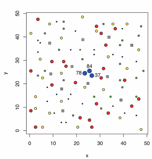
Figure 1. Study region with the sampling locations and the generated data. Filled circles are 97 considerd locations. Size of circles indicates the proportion of their values. $\boxplus$’s indicate the hold-out dataset locations.

First of all, we draw a sample of size $108$ from the normal distribution with mean $3$ and variance $0.2$ and save these values into a vector named $\bf{x}$. From now on, we will look at these data as a fixed (not random) and true values of a single covariate $x$. Then, we set parameters ${\beta_{0}}=0.5$, ${\beta_{1}}=2$, ${\sigma^{2}}=1$ and using an isotropic exponential covariance function with range parameter equal to $1.2$, we simulate a spatial dataset as a sample of response $Y\left(\cdot\right)$ on 108 considered locations with the linear trend ${\beta_{0}}+{\beta_{1}}{x\left({{s_{i}}}\right)}$. By leaving the above-mentioned $11$ locations and their related dataset, we use the rest of the dataset of size $97$ to fit the model. Since we investigated the potential of the proposed model to identify outliers, three locations ($37,78,84$) are selected and then contaminated adding $5$ units to the simulated data. From figure 1, one may observe a schematic description of the region that displays the sampling locations and the simulated data amounts.

[Figure 1 about here.]

In order to incorporate measurement error in the covariate $x$, after generating $\bf{u}$ as a sample of size 97 from $N\left(0,0.1\right)$ and setting $\bf{w}={\bf{x}}-\bf{u}$, hereafter we assume that we have no information about ${\bf{x}}$ and $\bf{u}$, and just observed $\bf{w}$. The prior distributions are as follows: $\mbox{\boldmath$\beta$\unboldmath}\sim{N_{2}}\left({\underline{0},{10^{3}}{I_{2}}}\right)$, ${\sigma^{2}}\sim HN\left({{0.02}}\right)$, ${\tau^{2}}\sim GIG\left({0,0.1,0.02}\right)$, ${\nu}\sim GIG\left({0,1,0.9}\right)$ and $\theta\sim Exp\left({0.82}\right)$. To implement computer programming using the publicly available R software, we need to set some initial (basic) values, so, for the two considered models, we set: $\beta_{0}=1.5$, $\beta_{1}=3$, $\sigma^{2}=2.8$, $\tau^{2}=3$, $\nu=0.1$, $\theta=5$ and the initial values for the latent variables $\varepsilon$ and $u$ are two samples of size 97 which have been generated from ${\varepsilon_{i}}\stackrel{{\scriptstyle iid}}{{\sim}}N\left({0,0.31}\right)$ and ${v_{i}}\stackrel{{\scriptstyle iid}}{{\sim}}N\left({0,0.31}\right)$, respectively.

Following consisting of comparing the performance of the GLG model with the Gaussian model $Y\left({s_{i}}\right)={\beta_{0}}+{\beta_{1}}{w}{\left({s_{i}}\right)}+\sigma{{\varepsilon\left({s_{i}}\right)}}-{\sigma_{u}}{\beta_{1}}u{\left({s_{i}}\right)}$, GM, hereafter. Results are based on $50,000$ draw from an MCMC chain after a burning period of $25,000$ iterations in which the taken lag value was $10$ to avoid the correlation problem in the generated chains. Convergence of the MCMC was verified through the Gelman and Rubin convergence diagnostics [1] using the R package coda. the Gelman and Rubin convergence diagnostics indicated convergence for each parameter and for a sample of the elements of the latent process. The results of models fitting are given in Table 1. According to this table, it is found that the value of DIC criterion for Gaussian log-Gaussian model is smaller than Gaussian model and it shows that the GLG model has a better performance.

[Table 1 about here.]

We now compare predictive performance of the two models Gaussian and GLG using the hold-out dataset. Here, we predicted $Y\left(s_{0_{i}}\right)$ for each sampling site $s_{0_{i}}$ in $11$ hold-out locations and then obtained the mean square error $\left({=\frac{1}{{11}}\sum\limits_{i=1}^{11}{{{\left[{Y\left({{s_{{0_{i}}}}}\right)-\widehat{Y\left({{s_{{0_{i}}}}}\right)}}\right]}^{2}}}}\right)$ the two models Gaussian and GLG as $3.5414$ and $0.2615$, respectively. So, the GLG model outperforms the response.

In the prior sensitivity analysis of the GLG model, we monitor the posterior distributions, focusing in one parameter at a time, say in parameter $\phi$, where its prior has been modified at that time. The absolute value of the induced change in the marginal posterior mean of $\phi$ divided by the standard deviation computed under the benchmark prior, is a simple measure which is named relative change and determines how the resulting posterior has changed. Whenever $\phi$ is a vector, the relative change is calculated for each element and the maximum relative change across elements is then reported. From Table 2, one can see list of the various values used for the alternative prior hyperparameters and the maximum (across priors) relative change as well, recorded for each parameter. This Table shows that the prior on the model parameters $\beta$ and $\sigma^{2}$ does not appear to play a very critical role in the presence of measurement error. However the prior on $\tau^{2}$ and $\theta$ is more important than the above-mentioned parameters, prior on $\tau^{2}$ is most noteworthy because of its effect on the inference on $\sigma^{2}$. Lastly, the influence of prior changes on $\nu$ is far and away the largest prior effect that occurs in this sensitivity analysis. This was not an unexpected subject from inception because the model by itself would be unable to demonstrate the treatment of the latent parameters. Table 3 which lists some alternatives basic values used for the sensitivity checking to the initials (in the GLG model) and their maximum relative changes as well, confirm that there is no longer any serious worry about the sensitivity to the initial values.

[Table 2 about here.]

[Table 3 about here.]

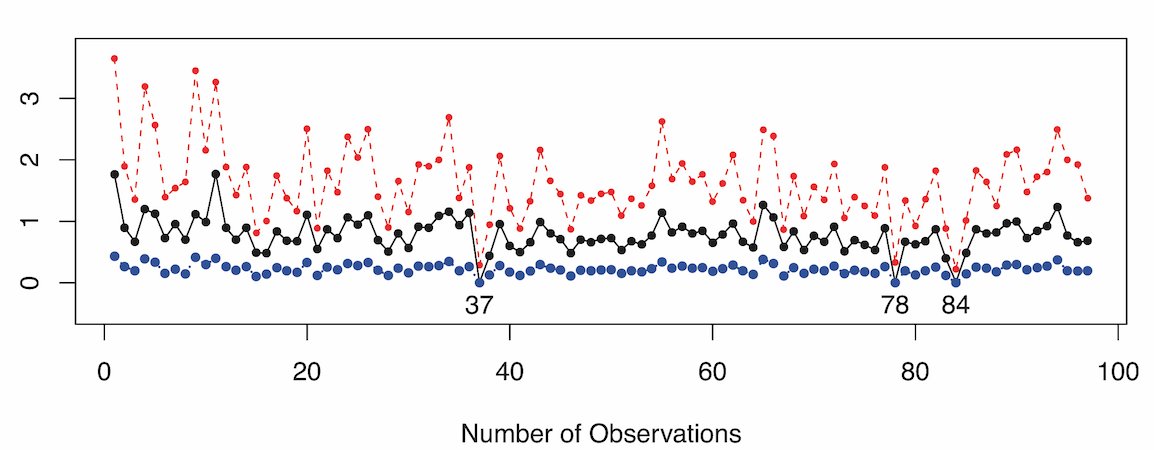
Figure 2. The HPD regions and the estimated values of $E\left(\lambda_{i}\left|{\bf y}\right.\right)$ under the GLG model. Dotted line: lower bound. Solid line: $E\left(\lambda\left|{\bf y}\right.\right)$. Dashed line: upper bound.

Now we intend to assess the ability of the proposed model to correctly identify outlying observations using the simulated data and the identifiability of the parameters as well. Although following Palacios and Steel [12] we can compute the Bayes factor in order to identify the outliers, this method is not computationally efficient. We against apply the Chen-Shao algorithm [8] to obtain the $95\%$ highest posterior density (HPD) credible intervals of $\lambda_{i}$. Figure 2 which presents the $95\%$ HPD regions and the posterior mean values of $\lambda_{i}$, confirms that three observations $37,78$ and $84$ have the smallest posterior mean values of mixing variables and very small HPD intervals.

[Figure 2 about here.]

Since the proposed model introduces the extra parameter $\tau^{2}$ beyond the parameterization of the GLG model (without measurement error), it is natural to examine to what extent information on this parameter can be recovered from data. Now, in order to address parameters identifiability, we focus on the parameters $\sigma^{2}$ and $\tau^{2}$, because we would expect inference to be most challenging for these parameters and we generate three data sets with different values for them. Then, the estimates of the model parameters are obtained. Table 4 displays the results.

[Table 4 about here.]

4. Nitrate Concentration

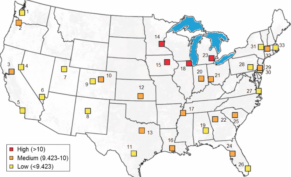
Figure 3. The nitrate concentration data (in $mg/L$) in the United States region. Filled boxes are 33 registration sites of monitoring.

Elevated nitrate concentrations in groundwater is a serious concern for governments around the world because groundwater provides drinking water for more than one-half of the Nation’s population [6], and is the sole source of drinking water for many rural communities and some large cities and nitrate is especially a problem as a contaminant in drinking water due to its harmful biological effects. The United States Environmental Protection Agency (EPA) established the current drinking water standard and health advisory level of $10mg/L$ nitrate based on the human health risks due to nitrate consumption. In this section which consists of an illustrative application of our methodology, we focus on nitrate pollution data come from a monitoring network composed of $33$ stations in $1990$ around the United States. The data contains nitrate ($\rm{NO_{3}^{-}}$), nitrite ($\rm{NO_{2}^{-}}$) and ammonium ($\rm{NH_{4}^{+}}$) concentration in $mg/L$, with $1mg/L$ and $0.5mg/L$ standard as the maximum contaminant levels, respectively, and also spatial coordinates in degrees. Figure 3 shows a schematic description of the region, locations of the stations and the nitrate concentration.

[Figure 3 about here.]

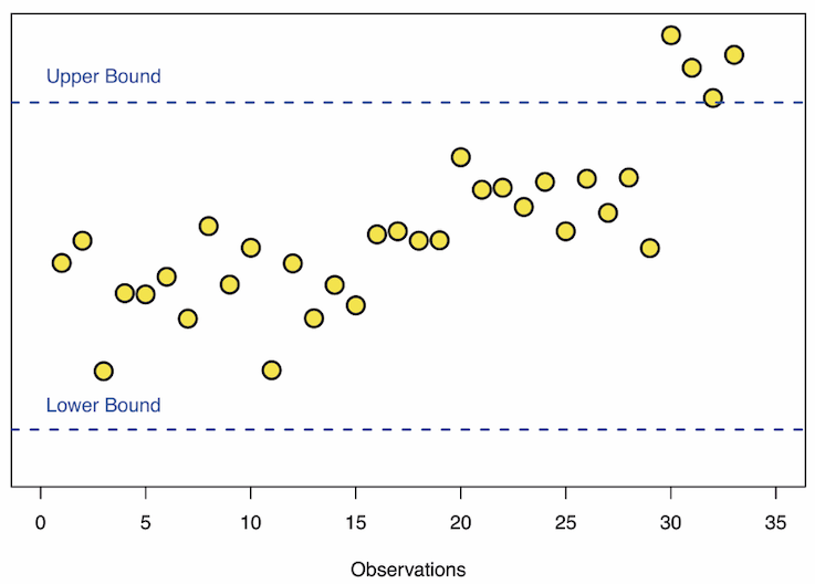
Figure 4. The Haining bounds.

As can easily be seen in this Figure, four locations $14,15,18$ and $23$ which are next to each other, have larger values compared to the rest. In fact, we are faced with a region with larger observational variance relative to the rest. To our knowledge, measuring the $\rm{NO_{2}^{-}}$ and $\rm{NH_{4}^{+}}$ concentration in groundwater is faced with measurement error, and so these aspects not only justify our methodology, but they are also a relevant issue for statistical applications. The main aims are to provide a reasonable prediction map based on information contained in the data. For this purpose, we view the data as a partial realization from a random field. Our initial exploratory analysis which was performed based on Haining method on outlier detection, confirms the existence of a region in the space with larger observational variance (Figure 4). The histogram and Q-Q plot of these data which have been shown in Figure 5 show a violation of the assumption of Gaussianity.

[Figure 4 about here.]

[Figure 5 about here.]

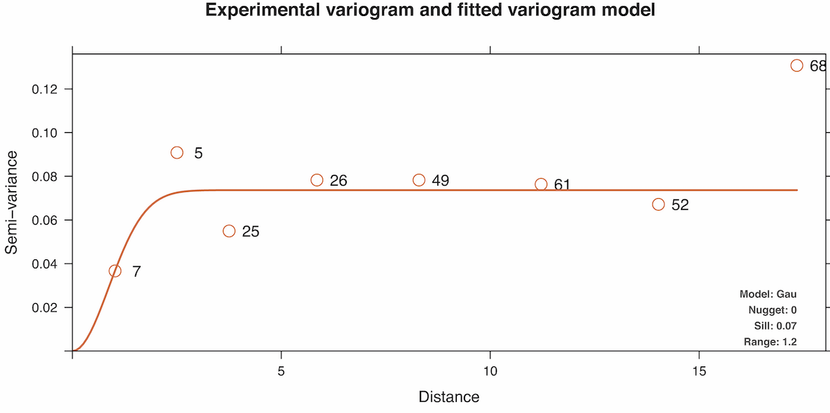
Figure 6. Robust empirical semivariograms.

[Figure 6 about here.]

Roughly speaking, plots of the empirical directional semivariograms (not shown here) provide no indication of the presence of anisotropy. Figure 6 which shows the highly robust empirical semivariogram [10] of data, confirms that there exists a strong spatial correlation as well as no nugget effect in the data set. To fit the linear model considered in this paper, we used the software package WinBUGS which has enabled complex models, that would be difficult or impossible to fit classically, to be fitted relatively straightforwardly using MCMC methods. The approach, based on Gibbs sampling, successively samples from the full conditional distribution of each parameter, given values of all other parameters in the model. Although the model we considered is a fairly complex model, WinBUGS is an efficient tool in such cases. The prior distributions are as follows: $\mbox{\boldmath$\beta$\unboldmath}\sim{N_{3}}\left({0,{{10}^{4}}{I_{3}}}\right)$, ${\sigma^{2}}\sim HN\left({{10}^{-2}}\right)$, ${\tau^{2}}\sim Inv-Gamma\left(1,{0.2}\right)$, ${\nu}\sim Inv-Gamma\left(1,{0.2}\right)$ and $\theta\sim Exp\left({0.85}\right)$.

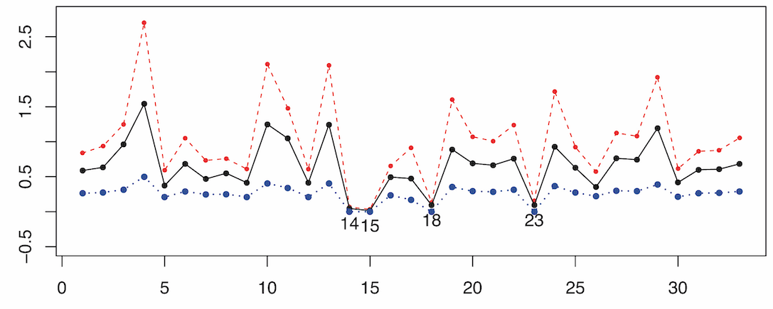
Figure 7. The HPD regions and the estimated values of $E\left(\lambda_{i}\left|{\bf y}\right.\right)$ under the GLG model. Dotted line: lower bound. Solid line: $E\left(\lambda\left|{\bf y}\right.\right)$. Dashed line: upper bound.

Table 5 reports the parameters estimation, their estimated variances and also their Monte Carlo error [2] under the GLG model. Figure 7 presents the $95\%$ HPD regions and the posterior mean values of ${\lambda_{i}}$ for $i=1,\ldots,33$ under the GLG model. As seen, the smallest posterior mean values of mixing variables were found to correspond to observations $14,15,18$ and $23$.

[Table 5 about here.]

[Figure 7 about here.]

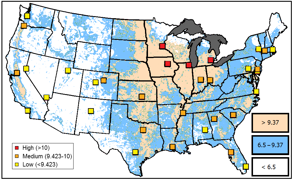
Figure 8. Map of predicted nitrate concentration.

Finally, the predictive map under the GLG model is shown in figure 8. According to this figure, the predictions are highest in the area which contains the aforementioned observations.

[Figure 8 about here.]

5. Conclusion

In this paper, we have proposed a spatial linear measurement error model to account for covariate measurement error and spatial correlation in spatial data. For this purpose, we adopted the Bayesian approach and utilized the Markov chain Monte Carlo algorithms and data augmentations to carry out calculations. Using simulated data, meaningful inference on parameters, prediction, sensitivity to the priors and identifiability was concluded.

Since all covariates in nitrate concentration faced with instrumental measurement error, this problem indicates that our methodology is well-suited to analyze these data. Obviously, the conclusions and the final suggestion in our case study do not constitute the general answer to the question about the best choice of computational methods. Recently, some studies have been performed to find replacing methods and it has led to new methods. For example, the Variational Bayes method is one of the most ones. Although this method requires more complex theoretic calculations, it could increase the speed of calculations.

As can be seen in Appendix, the elements of $\psi$ are not conditionally independent given other parameters and data and so in view of the large dimension of $\psi$ to dominate complexity, Palacios and Steel [12] partitioned the elements of $\psi$ in blocks, each of which corresponds to a cluster of observations that are relatively close together. Assessing the performance of this method is an interesting area to investigate in further research.

Appendix: The Conditional Distributions

Below is the full conditional distributions of all unobservable quantities to draw samples from $P\left({\mbox{\boldmath$\lambda$\unboldmath},\mbox{\boldmath$\varepsilon$\unboldmath},\eta\left|{\bf y}\right.}\right)$ in the Gibbs sampler framework. In what follows, we use the notation ${{\eta_{-\phi}}}$ to show the vector $\eta$ without $\phi$. Regardless of the details, the full conditional distributions are as follows:

• Latent variable $\psi$
  For each of the components of $\psi$ we can write

  $$P\left({{\psi_{i}}\left|{{\bf{y}},{\mbox{\boldmath$\psi$\unboldmath}_{-i}},\mbox{\boldmath$\varepsilon$\unboldmath},\eta}\right.}\right)\propto P\left({{\bf{Y}}\left|{\mbox{\boldmath$\psi$\unboldmath},\mbox{\boldmath$\varepsilon$\unboldmath},\eta}\right.}\right)P\left({{\psi_{i}}\left|{{\mbox{\boldmath$\psi$\unboldmath}_{-i}},\mbox{\boldmath$\varepsilon$\unboldmath},\eta}\right.}\right),$$ (7)

  where the first term in the above equation (i.e., the likelihood contribution) is proportional to product of probability density functions normal distribution truncated to $\left[0,\infty\right)$. To construct a suitable candidate generator, as recommended by Palacios and Steel [12], we approximate this distribution by log-normal distributions on $\lambda_{i}$. By matching the first two moments of $\lambda_{i}$ , we obtain, as an approximating distribution of the likelihood contribution to $\psi_{i}$, as, ${\psi_{i}}\left|{\varepsilon_{i}},\eta\right.\sim N\left({{m_{i}},s_{i}^{2}}\right)$, where ${m_{i}}=\ln\frac{{\varepsilon_{i}^{2}\left[{1+{h_{i}}\delta\left({{h_{i}}}\right)+h_{i}^{2}}\right]}}{{{\tau^{2}}{{\mbox{\boldmath$\beta$\unboldmath}}_{x}^{\prime}}{\mbox{\boldmath$\beta$\unboldmath}_{x}}{{\left[{\delta\left({{h_{i}}}\right)+{h_{i}}}\right]}^{4}}}}$, ${s_{i}^{2}}=4\ln\frac{{1+{h_{i}}\delta\left({{h_{i}}}\right)+h_{i}^{2}}}{{{{\left[{\delta\left({{h_{i}}}\right)+{h_{i}}}\right]}^{2}}}}$, $\delta\left({\cdot}\right)=\frac{{\phi\left({\cdot}\right)}}{{\Phi\left({\cdot}\right)}}$, $h_{i}=\frac{{{t_{{1_{i}}}}sign\left({{\varepsilon_{i}}}\right)}}{{\tau{{\left({{{\mbox{\boldmath$\beta$\unboldmath}}_{x}^{\prime}}{\mbox{\boldmath$\beta$\unboldmath}_{x}}}\right)}^{\frac{1}{2}}}}}$ and ${{\bf{t}}_{1}}=\frac{1}{\sigma}\left(\bf{y}-{{\rm W}^{*}}{\mbox{\boldmath$\beta$\unboldmath}}\right)$. Combining $\pi\left({{\psi_{i}}\left|{{\mbox{\boldmath$\psi$\unboldmath}_{-i}}}\right.}\right)\sim N\left({m_{i}^{*},s_{i}^{{*^{2}}}}\right)$ and $P\left({\psi_{i}}\left|{\varepsilon_{i}},\eta\right.\right)$, where $m_{i}^{*}$ and $s_{i}^{{*^{2}}}$ could be drive easily, we propose a candidate value for $\psi_{i}$, say $\psi_{i}^{cand}$ from

  $${\psi_{i}}\left|{{\bf{y}},{\mbox{\boldmath$\psi$\unboldmath}_{-i}},\mbox{\boldmath$\varepsilon$\unboldmath},\eta}\right.\sim N\left({\frac{{s_{i}^{2}m_{i}^{*}+s_{i}^{{*^{2}}}{m_{i}}}}{{s_{i}^{2}+s_{i}^{{*^{2}}}}},\frac{{s_{i}^{2}s_{i}^{{*^{2}}}}}{{s_{i}^{2}+s_{i}^{{*^{2}}}}}}\right).$$

• Latent variable $\varepsilon$
  Let ${{{t}}_{{1_{i}}}^{*}}={t_{{1_{i}}}}\sqrt{{\lambda_{i}}}$ for $i=1,2,\ldots,n$ and ${{A_{1}}=C_{\theta}^{-1}+\frac{{{\Lambda^{-1}}}}{{{\tau^{2}}{{\mbox{\boldmath$\beta$\unboldmath}}_{x}^{\prime}}{\mbox{\boldmath$\beta$\unboldmath}_{x}}}}}$. we obtain $\mbox{\boldmath$\varepsilon$\unboldmath}\left|{{\bf{y}},\mbox{\boldmath$\lambda$\unboldmath},\eta}\right.\sim{N_{n}}\left({A_{1}^{-1}{\bf{t}}_{1}^{*},A_{1}^{-1}}\right)$.

• The intercept
  The conditional distribution of the intercept parameter is obtained as

  $$N\left({\frac{1}{{\frac{n}{{{\tau^{2}}{\sigma^{2}}{{\mbox{\boldmath$\beta$\unboldmath}}_{x}^{\prime}}{\mbox{\boldmath$\beta$\unboldmath}_{x}}}}+\frac{1}{{{c_{1}}}}}}\frac{{\sum\limits_{i=1}^{n}{{t_{{2_{i}}}}}}}{{{\tau^{2}}{\sigma^{2}}{{\mbox{\boldmath$\beta$\unboldmath}}_{x}^{\prime}}{\mbox{\boldmath$\beta$\unboldmath}_{x}}}},\frac{1}{{\frac{n}{{{\tau^{2}}{\sigma^{2}}{{\mbox{\boldmath$\beta$\unboldmath}}_{x}^{\prime}}{\mbox{\boldmath$\beta$\unboldmath}_{x}}}}+\frac{1}{{{c_{1}}}}}}}\right),$$

  by setting ${{\bf{t}}_{2}}={\bf{y}}-{\rm W}{\mbox{\boldmath$\beta$\unboldmath}_{x}}-\sigma\frac{\mbox{\boldmath$\varepsilon$\unboldmath}}{{\sqrt{\mbox{\boldmath$\lambda$\unboldmath}}}}$.

• Parameter $\tau^{2}$

  $${{\tau^{2}}\left|{{\bf{y}},\mbox{\boldmath$\lambda$\unboldmath},\mbox{\boldmath$\varepsilon$\unboldmath},{\eta_{-{\tau^{2}}}}}\right.}\sim GIG\left({-\frac{n}{2},{\sqrt{c_{3}^{2}+\frac{{\sum\limits_{i=1}^{n}{{{\left({{t_{{2_{i}}}}-{\beta_{0}}}\right)}^{2}}}}}{{{\sigma^{2}}{{\mbox{\boldmath$\beta$\unboldmath}}_{x}^{\prime}}{\mbox{\boldmath$\beta$\unboldmath}_{x}}}}}},{c_{4}}}\right).$$

In the four last items, the full conditional distribution of parameters $\mbox{\boldmath$\beta$\unboldmath}_{x}$, $\sigma^{2}$, $\nu$ and $\theta$ are of nonstandard form, so a Metropolis-Hastings step or sampling- importance resampling (SIR) algorithm would be used. By choosing the SIR algorithm to draw samples from an unknown quantitiy, say $\phi$, first, an independent random sample $\left\{{{\phi_{{j}}}}\right\}_{j=1}^{m}$ is drawn from a proposal distribution $q$. A conservative candidate distribution for applying the SIR algorithm is the pre-specified prior on $\phi$. Then, second, a smaller sample is drawn with replacement from them with sample probabilities ${p_{j}}=\frac{{L\left({data\left|{{\phi_{{j}}}}\right.}\right)}}{{\sum\limits_{j}{L\left({data\left|{{\phi_{{j}}}}\right.}\right)}}}$, where ${L\left({data\left|{{\phi_{{j}}}}\right.}\right)}$ denotes the likelihood contribution in the full conditional distribution of $\phi$.

• Parameter $\mbox{\boldmath$\beta$\unboldmath}_{x}$
  If ${t_{{3_{i}}}}={y_{i}}-{\beta_{0}}-\sigma\frac{{{\varepsilon_{i}}}}{{\sqrt{{\lambda_{i}}}}}$ for $i=1,2,\ldots n$, then $\pi\left({{\mbox{\boldmath$\beta$\unboldmath}_{x}}\left|{{\bf{y}},\mbox{\boldmath$\lambda$\unboldmath},\mbox{\boldmath$\varepsilon$\unboldmath},{\eta_{-{\mbox{\boldmath$\beta$\unboldmath}_{x}}}}}\right.}\right)$ is proportional to

  $${\left({\frac{1}{{{{\mbox{\boldmath$\beta$\unboldmath}}_{x}^{\prime}}{\mbox{\boldmath$\beta$\unboldmath}_{x}}}}}\right)^{\frac{n}{2}}}\exp\left\{{-\frac{{{{\mbox{\boldmath$\beta$\unboldmath}}_{x}^{\prime}}{{\rm W}^{*}}^{\prime}{{\rm W}^{*}}{\mbox{\boldmath$\beta$\unboldmath}_{x}}-2{{\mbox{\boldmath$\beta$\unboldmath}}_{x}^{\prime}}{{\rm W}^{*}}^{\prime}{{\bf{t}}_{3}}}}{{2{\tau^{2}}{\sigma^{2}}{{\mbox{\boldmath$\beta$\unboldmath}}_{x}^{\prime}}{\mbox{\boldmath$\beta$\unboldmath}_{x}}}}}{-\frac{1}{{2{c_{1}}}}{{\mbox{\boldmath$\beta$\unboldmath}}_{x}^{\prime}}{\mbox{\boldmath$\beta$\unboldmath}_{x}}}\right\}$$

  and ${L\left({data\left|{{\beta_{{x_{j}}}}}\right.}\right)}={\left({\frac{1}{{{{\mbox{\boldmath$\beta$\unboldmath}}_{x}^{\prime}}{\mbox{\boldmath$\beta$\unboldmath}_{x}}}}}\right)^{\frac{n}{2}}}\exp\left\{{-\frac{{{{\mbox{\boldmath$\beta$\unboldmath}}_{x}^{\prime}}{{\rm W}^{*}}^{\prime}{{\rm W}^{*}}{\mbox{\boldmath$\beta$\unboldmath}_{x}}-2{{\mbox{\boldmath$\beta$\unboldmath}}_{x}^{\prime}}{{\rm W}^{*}}^{\prime}{{\bf{t}}_{3}}}}{{2{\tau^{2}}{\sigma^{2}}{{\mbox{\boldmath$\beta$\unboldmath}}_{x}^{\prime}}{\mbox{\boldmath$\beta$\unboldmath}_{x}}}}}\right\}$.

• Parameter $\sigma^{2}$
  $\pi\left({{\sigma^{2}}\left|{{\bf{y}},\mbox{\boldmath$\lambda$\unboldmath},\mbox{\boldmath$\varepsilon$\unboldmath},{\eta_{-{\sigma^{2}}}}}\right.}\right)$ is proportional to

  $${\left({\frac{1}{{{\sigma^{2}}}}}\right)^{\frac{n}{2}}}\exp\left\{-\frac{{{{\left({{c_{2}}{\sigma^{2}}}\right)}^{2}}}}{\pi}{-\frac{1}{{2{\sigma^{2}}{\tau^{2}}{{\mbox{\boldmath$\beta$\unboldmath}^{\prime}}_{x}}{\mbox{\boldmath$\beta$\unboldmath}_{x}}}}\sum\limits_{i=1}^{n}{{{\left({{t_{{4_{i}}}}-\sigma\frac{{{\varepsilon_{i}}}}{{\sqrt{{\lambda_{i}}}}}}\right)}^{2}}}}\right\},$$

  in which ${{\bf{t}}_{4}}={\bf{y}}-{{\rm W}^{*}}\mbox{\boldmath$\beta$\unboldmath}$ and ${L\left({data\left|{\sigma_{j}^{2}}\right.}\right)}={{{{\sigma_{j}^{-n}}}}}\exp\left\{{-\frac{\sum\limits_{i=1}^{n}{{{\left({{t_{{4_{i}}}}-\frac{{{\sigma_{j}}{\varepsilon_{i}}}}{{\sqrt{{\lambda_{i}}}}}}\right)}^{2}}}}{{2{\sigma_{j}^{2}}{\tau^{2}}{{\mbox{\boldmath$\beta$\unboldmath}}_{x}^{\prime}}{\mbox{\boldmath$\beta$\unboldmath}_{x}}}}}\right\}.$

• Parameter $\nu$
  We can write the full conditional distribution $\pi\left({\nu\left|{{\bf{y}},\mbox{\boldmath$\lambda$\unboldmath},\mbox{\boldmath$\varepsilon$\unboldmath},{\eta_{-\nu}}}\right.}\right)$ in proportion to

  $$\frac{1}{{{\nu^{\frac{n}{2}+1}}}}\exp\left\{{-\frac{1}{{2\nu}}{{\left({\ln\mbox{\boldmath$\lambda$\unboldmath}+\frac{\nu}{2}J}\right)}^{\prime}}C_{\theta}^{-1}\left({\ln\mbox{\boldmath$\lambda$\unboldmath}+\frac{\nu}{2}J}\right)}{-\frac{1}{2}\left[{\frac{{c_{5}^{2}}}{\nu}+c_{6}^{2}\nu}\right]}\right\},$$

  and so we are able to use the SIR algorithm with probabilities

  $${p_{j}}=\frac{{\nu_{j}^{-\frac{n}{2}}\exp\left\{{-\frac{1}{{2{\nu_{j}}}}{{\left({\ln{{\mbox{\boldmath$\lambda$\unboldmath}}}+\frac{{{\nu_{j}}}}{2}J}\right)}^{\prime}}C_{\theta}^{-1}\left({\ln{{\mbox{\boldmath$\lambda$\unboldmath}}}+\frac{{{\nu_{j}}}}{2}J}\right)}\right\}}}{{\sum\limits_{j=1}^{m}{\nu_{j}^{-\frac{n}{2}}\exp\left\{{-\frac{1}{{2{\nu_{j}}}}{{\left({\ln{{\mbox{\boldmath$\lambda$\unboldmath}}}+\frac{{{\nu_{j}}}}{2}J}\right)}^{\prime}}C_{\theta}^{-1}\left({\ln{{\mbox{\boldmath$\lambda$\unboldmath}}}+\frac{{{\nu_{j}}}}{2}J}\right)}\right\}}}}.$$

• Parameter $\theta$

  $$\pi\left({\theta\left|{{\bf{y}},\mbox{\boldmath$\lambda$\unboldmath},\mbox{\boldmath$\varepsilon$\unboldmath},{\eta_{-\theta}}}\right.}\right) \propto \exp\left\{{-\frac{1}{{2\nu}}{{\left({\ln\mbox{\boldmath$\lambda$\unboldmath}+\frac{\nu}{2}J}\right)}^{\prime}}C_{\theta}^{-1}\left({\ln\mbox{\boldmath$\lambda$\unboldmath}+\frac{\nu}{2}J}\right)}\right\}$$

  $$\times\exp\left\{{-\frac{1}{2}\mbox{\boldmath$\varepsilon$\unboldmath}^{\prime}C_{\theta}^{-1}\mbox{\boldmath$\varepsilon$\unboldmath}}\right\}{\nu^{-\frac{n}{2}}}{\left|{{C_{\theta}}}\right|^{-1}}$$

  $$\hskip 25.60747pt\times\exp\left\{{-\frac{{{c_{8}}}}{{med\left(d\right)}}\theta}\right\}.$$

  Since this full conditional distribution is of nonstandard form as well, so the SIR algorithm would be used again.

Table 1. The estimated value (EVal) and the estimated variance (EVar) of parameters and DIC criterion based on Gaussian and Gaussian log-Gaussian models.

		Gaussian		GLG
Parameter	Real value	EVal	EVar	EVal	EVar
${\beta_{0}}$	$0.5$	$-0.0521$	$1.7876$	$0.4286$	$0.7137$
${\beta_{1}}$	$2$	$3.112$	$2.2069$	$1.864$	$0.087$
${\sigma^{2}}$	$1$	$3.3652$	$2.8361$	$1.2504$	$1.4312$
${\tau^{2}}$	$0.1$	$1.63$	$1.9076$	$0.455$	$0.903$
$\nu$	$1$	-	-	$0.9781$	$1.8413$
$\theta$	$1.2$	$4.3619$	$2.8021$	$1.418$	$1.3056$
DIC		$367.07$		$295.11$

Table 2. Prior sensitivity analysis of the GLG model: setup of the experiment and maximum relative change (MRC).

Parameter	Hyperparameter	Benchmark	Alternatives	MRC
$\beta$	$c_{1}$	$10^{3}$	$10^{2},10^{4}$	$0.0206$
${\sigma^{2}}$	${c_{2}}$	$0.02$	$0.01,0.04$	$0.1718$
${\tau^{2}}$	$\left({c_{3}},{c_{4}}\right)$	$\left({0.1},{0.02}\right)$	$\left({0.2},{0.03}\right),\left({0.05},{0.01}\right)$	$0.3864$
$\nu$	$\left({c_{5}},{c_{6}}\right)$	$\left({1},{0.9}\right)$	$\left(0.5,1.1\right),\left(1.2,0.1\right)$	$3.021$
$\theta$	$c_{7}$	$0.82$	$0.71,1.18$	$0.6254$

Table 3. Initial sensitivity analysis of the GLG model: setup of the experiment and maximum relative change (MRC).

Parameter	Real value	Initial value	Alternatives	MRC
$\beta_{0}$	$0.5$	$1.5$	$0.2$ , $2.1$	$0.0117$
$\beta_{1}$	$2$	$3$	$1.11$ , $2.6$	$0.0183$
$\sigma^{2}$	$1$	$2.8$	$0.5$ , $1.5$	$0.0922$
$\tau^{2}$	$0.1$	$3$	$0.75$ , $1.3$	$0.1471$
$\nu$	$1$	$0.1$	$0.6$ , $1.4$	$0.2942$
$\theta$	$1.2$	$5$	$0.9$ , $1.05$	$0.233$

Table 4. Identifiability of the parameters $\sigma^{2}$ and $\tau^{2}$.

$\sigma^{2}$	True value	$0.74$	$1.1$	$1.28$
	Estimated value	$1.198$	$0.911$	$1.704$
$\tau^{2}$	True value	$0.08$	$0.1$	$0.19$
	Estimated value	$0.365$	$0.387$	$0.469$

(a)

(b)

Figure 5. (a) Histogram, (b) Q-Q plot.

Table 5. The estimated value (EVal), the estimated variance (EVar) and the Monte Carlo error (MC error) of parameters based on Gaussian log-Gaussian model.

Parameter	EVal	EVar	MC error
$\beta_{0}$	$7.988$	$0.858$	$0.02958$
$\beta_{1}$	$1.497$	$0.071$	$0.01837$
$\beta_{2}$	$0.5123$	$0.0923$	$0.01578$
$\sigma^{2}$	$2.526$	$1.8871$	$0.01817$
$\tau^{2}$	$0.981$	$1.5206$	$0.1413$
$\nu$	$1.86$	$1.9214$	$0.7338$
$\theta$	$0.9894$	$1.2984$	$0.09601$

References

• [1] Andrew Gelman and Donald B Rubin. Inference from iterative simulation using multiple sequences. Statistical science, pages 457–472, 1992.
• [2] I. Ntzoufras. Bayesian modeling using WinBUGS, volume 698. John Wiley & Sons, 2011.
• [3] Vahid Tadayon. Bayesian analysis of censored spatial data based on a non-gaussian model. Journal of Statistical Research, , 13 (2), 155-180,  2017.
• [4] S. M. Berry, R. J. Carroll, and D. Ruppert. Bayesian smoothing and regression splines for measurement error problems. Journal of the American Statistical Association, 97(457):160–169, 2002.
• [5] Vahid Tadayon. Analysis of gaussian spatial models with covariate measurement error. arXiv preprint arXiv:1811.05648, 2018.
• [6] Wayne B Solley, Robert R Pierce, and Howard A Perlman. Estimated use of water in the United States in 1995, volume 1200. US Geological Survey, 1998.
• [7] Vahid Tadayon. On an extension of stochastic approximation em algorithm for incomplete data problems.   arXiv preprint arXiv:1811.08595, 2018.
• [8] Ming-Hui Chen and Qi-Man Shao. Monte carlo estimation of bayesian credible and hpd intervals. Journal of Computational and Graphical Statistics, 8(1):69–92, 1999.
• [9] Vahid Tadayon and Majid Jafari Khaledi. Bayesian analysis of skew Gaussian spatial models based on censored data. Communications in Statistics-Simulation and Computation, 44(9):2431–2441, 2014.
• [10] Marc G Genton. Highly robust variogram estimation. Mathematical Geology, 30(2):213–221, 1998.
• [11] Vahid Tadayon and Abdolrahman Rasekh. Non-Gaussian covariate-dependent spatial measurement error model for analyzing big spatial data. Journal of Agricultural, Biological and Environmental Statistics,   doi: 10.1007/s13253-018-00341-3, 2018.
• [12] M. B. Palacios and M. F. J. Steel. Non-gaussian bayesian geostatistical modeling. Journal of the American Statistical Association, 101(474):604–618, 2006.
• [13] Vahid Tadayon and Mahmoud Torabi. Spatial models for non-gaussian data with covariate measurement error. Environmetrics,   doi: 10.1002/env.2545, 2018.
• [14] C.V. Deutsch and A.G. Journel. GSLIB: Geostatistical Software Library and User’s Guide. Oxford University Press, New York, 1992.