A Fast Iterative Algorithm for High-dimensional Differential Network
Abstract
Differential network is an important tool to capture the changes of conditional correlations under two sample cases. In this paper, we introduce a fast iterative algorithm to recover the differential network for high-dimensional data. The computation complexity of our algorithm is linear in the sample size and the number of parameters, which is optimal in the sense that it is of the same order as computing two sample covariance matrices. The proposed method is appealing for high-dimensional data with a small sample size. The experiments on simulated and real data sets show that the proposed algorithm outperforms other existing methods.
Keywords: ADMM, Differential network, Gaussian graphical model, High-dimensional data, Precision matrix
1 Introduction
Covariance matrices which describe the correlations between covariates play an important role in multivariate statistical analysis. For high-dimensional data where the number of covariates is large, it is challenging to estimate the covariance matrix. In literature, a large number of statistical methods have been proposed to estimate the covariance matrix (Bickel and Levina, 2008; Rothman et al., 2009; Cai and Liu, 2011) or its inverse which is usually called as the precision matrix (Meinshausen and Bühlmann, 2006; Jerome et al., 2008; Cai et al., 2011; Zhang and Zou, 2014). More details can be found in recent review works by Tong et al. (2014) or Fan et al. (2016).
In this work, we study the covariance structure for the two-sample cases. Suppose that we have observations from two groups of subjects: and whose population covariance matrices are and , respectively. Our interest is to estimate the differential network , which is the difference between two precision matrices. In biostatistics, the differential network describes the changes of conditional interdependencies between components under different environmental or genetic conditions. See Barabási and Oltvai (2004), Bandyopadhyay et al. (2010), Barabási et al. (2011), Gambardella et al. (2013), and Zhao et al. (2014) for example and the references therein. Another application of the differential network is the quadratic discriminant analysis in multivariate statistical analysis (Anderson, 2003). Under the Gaussian distribution assumption, the differential network is exactly the coefficients for the interaction terms between covariates. For quadratic discriminant analysis, it is necessary to recover the differential network (Li and Shao, 2015; Jiang et al., 2018).
In the past decades, a large number of statistical methods have been proposed to estimate which can be classified into two categories. The first one is to estimate precision matrices and separately, and then taking the difference yields the final estimation for the differential network. The methods for estimating a single precision matrix (Meinshausen and Bühlmann, 2006; Jerome et al., 2008; Cai et al., 2011; Zhang and Zou, 2014) can be used directly. The second approach is to jointly estimate precision matrices and (Julien et al., 2011; Jian et al., 2011; Zhu and Li, 2018). A joint loss function for the precision matrices is conducted and we can estimate the precision matrices simultaneously by penalizing the joint loss function. These methods assume that each precision matrix is sparse and can be recovered consistently which is too strong for many applications. Moreover, since our interest is only the differential network, it is not necessarily to recover each network for all the subjects.
Recently, Zhao et al. (2014) developed a direct estimator for the differential network under high-dimensional setting. Motivated by Cai et al. (2011), they proposed a Dantzig-typed estimator for the high-dimensional differential network. By studying high-dimensional quadratic discriminant analysis, Jiang et al. (2018) proposed a LASSO-typed estimator which regularized a convex loss function with a penalized term. Usually, the estimators of Zhao et al. (2014) and Jiang et al. (2018) are not symmetric and a further symmetrical step is needed for the final estimation. Yuan et al. (2017) conducted an one step symmetric estimator. Under mild conditions, these estimators are all shown to be consistent by assuming that the differential network matrix is sparse. Computationally, they all used the alternating direction method of multipliers (ADMM) (Boyd et al., 2011) to solve the optimization problems. In details, Zhao et al. (2014) used a proximal linearizion procedure to solve the Dantzig-typed optimization problem. The penalized problem of Jiang et al. (2018) can be solved by standard ADMM and Yuan et al. (2017) proposed a two step ADMM algorithm.
For high-dimensional data where , the computational complexity of Zhao et al. (2014) is while Jiang et al. (2018) and Yuan et al. (2017) improved the complexity to . In this paper, we introduce a fast iterative shrinkage-thresholding algorithm (Beck and Teboulle, 2009) to minimize loss functions defined in Yuan et al. (2017) and Jiang et al. (2018). The computational complexity of the new method is improved to around , which is the same as computing the two sample covariance matrices. Moreover, the proposed iterative shrinkage-thresholding algorithm is a first order method which is based on the gradients and avoids calculating the inverse of matrices. The theoretical convergence rate is also given in this paper. Lastly, simulation studies and real data analysis justify the advantages of our algorithm. An R package of our method has been developed and is available at http://math.sjtu.edu.cn/faculty/chengwang/pub.html.
The rest of the paper is organized as follows. In Section 2, we introduce the loss functions in existing methods and propose the new algorithm. Evaluations in simulated data are presented in Section 3 and in Section 4, the algorithm is applied to two real data sets to demonstrate its performance. The theoretical convergence rate of the algorithm are proved in Appendix.
2 Main Results
For any real matrix , we shall use to denote its Frobenius norm, to denote its spectral norm and denotes the sum of the absolute values of .
2.1 Existing Methods
Our interest is to estimate the differential network which is defined as the difference between two precision matrices. Noting
| (2.1) |
we can get
where denotes the Kronecker product and is the vectorization of a matrix. To estimate , following LASSO (Tibshirani, 1996), we can consider the penalized estimation
where are the sample covariance matrices and is a tuning parameter. Letting , we can get the estimation in matrix form
| (2.2) |
which is exactly the estimator proposed by Jiang et al. (2018). Here, the loss function
| (2.3) |
is convex with respect to which is appealing for optimization. Generally, the estimation is not symmetric and a further symmetrization is needed to obtain the final estimator. Yuan et al. (2017) considered a symmetric loss function
| (2.4) |
and proposed a symmetric estimation
| (2.5) |
Theoretically, assuming is sparse, Jiang et al. (2018) and Yuan et al. (2017) show that and are consistent estimators for the true differential network . Computationally, the loss functions are convex functions and standard ADMM (Boyd et al., 2011) can be used to solve the estimation (2.2) or (2.5). In details, for the loss function or , the augmented Lagrangian function is
where is the step size of ADMM. The iterative scheme of ADMM is
where is an element-wise soft thresholding operator. The related subproblem dominates the computation of each iteration since the other two subproblems are easy enough to calculate. Since is convex, it is equivalent to consider the equation
For the estimation (2.2), the equation is
| (2.6) |
and solving (2.5) is related to the equation
| (2.7) |
The equation (2.6) can be solved efficiently with the computation complexity and the explicit solution can be found in the Proposition 1 of Jiang et al. (2018) or the Lemma 1 of Yuan et al. (2017). For the equation (2.7), to derive the explicit solution, it is inevitable to calculate the inverse of a matrix whose complexity is . To obtain a computationally efficient algorithm, Yuan et al. (2017) introduced an auxiliary iterative update which solves the equation (2.6) twice and then combines the two solutions. In summary, the computation complexity of Jiang et al. (2018) or Yuan et al. (2017) is and an eigenvalue decomposition is necessary which will demand high computation memory.
2.2 New Algorithms
In this paper, we introduce a fast iterative shrinkage-thresholding algorithm (Beck and Teboulle, 2009) to solve the penalized estimation (2.2) and (2.5). Compared with ADMM which needs to solve equations or equivalently calculate the inverse of matrices, the shrinkage-thresholding algorithm is a first order method which is only based on function values and gradient evaluations. Specially, for the estimation (2.2) or (2.5), the gradient can be solved efficiently and then the computational complexity can be improved to where . Under the high dimension small sample size setting where , the computation complexity is linear in the sample size and the number of parameters, which is the same as computing the two sample covariance matrices.
For the optimization problem,
we consider the quadratic approximation at a given point ,
| (2.8) |
where is the Lipschitz constant for the gradient . Since (2.8) is a strongly convex function with respect to , the unique minimizer of for given is
Thus, we can solve the optimization problem sequentially
By the gradient descent algorithm for the convex functions, the sequence converges to the solution and following Beck and Teboulle (2009), we can further use an accelerated scheme to speed up the convergence. Details of the algorithm is summarized in Algorithm 1.
The main computational burden of this algorithm is Step 2 which involves the multiplication of the matrices. Specially, we need to calculate the gradients
where are all matrices. If we implement the algorithm naively, the computational complexity will be which is the same as the one of Jiang et al. (2018) or Yuan et al. (2017). For the high-dimensional data where , we have the formulas
where are the centered data matrix for the two subjects, respectively. Then the gradient can be calculated efficiently by using the facts
where the computational complexity can be reduced to .
For the fast iterative shrinkage-thresholding algorithm with accelerated scheme, the sequence of function values can converge to the optimal value at a linear convergence rate. That is , which is the best iteration complexity when only first order information is used (Nesterov, 1983). The following theorem gives the iteration complexity for the Algorithm 1 whose proof is postponed to Appendix for the sake of clarity.
Theorem 2.1
Let be generated by Algorithm 1 and . Then, for any ,
3 Simulation Studies
In this section, we conduct several simulations to demonstrate the performance of the proposed algorithm. In what follows, we refer to the method of Zhao et al. (2014) as “Dantzig”, the ADMM algorithm of Jiang et al. (2018) as “ADMM1” and the ADMM algorithm of Yuan et al. (2017) as “ADMM2”. The new proposed iterative shrinkage-thresholding algorithm are denoted as “New1” and “New2”. All the algorithms are terminated under the same stop condition .
For all of our simulations, we set the sample size and generate the data and from and , respectively. The true differential network is
and for the precision matrix , we consider two covariance structures:
-
•
Sparse case: . In details, and for all other . and for all other ;
-
•
Asymptotic sparse case: .
Table 1 summaries the computation time in seconds based on 10 replications where all methods are implemented in R with a PC with 3.40 GHz Intel Core i7-6700 CPU and 24GB memory. For all the methods, we solve a solution path corresponding to 50 lambda values ranging from to where is the maximum absolute elements of the differential sample covariance matrices corresponding to the estimation . From Table 1 we can see that for large , our proposed algorithms are much faster than the original ADMM methods whose complexity is and also the “Dantzig” method whose complexity is . Specially, based on ADMM, solving the symmetric estimation (2.5) is slower than calculating the estimation (2.2) since ADMM2 need to solve the equation (2.6) twice while ADMM1 only need to calculate (2.6) once. For the proposed shrinkage-thresholding algorithm, we can see that calculating the symmetric estimation uses less time which means the symmetry property help us get faster convergence rate.
| p=100 | p=200 | p=400 | p=600 | p=800 | |
| Sparse case | |||||
| Dantzig | 840.512(6.364) | ||||
| ADMM1 | 0.459(0.117) | 2.447(0.959) | 25.691(9.047) | 139.242(43.760) | 521.075(111.573) |
| ADMM2 | 1.748(0.384) | 8.879(1.146) | 62.252(11.657) | 272.317(57.756) | 847.754(59.007) |
| New1 | 0.773(0.158) | 1.819(0.318) | 8.984(1.795) | 26.505(9.277) | 94.504(28.198) |
| New2 | 0.702(0.104) | 1.797(0.205) | 8.263(1.284) | 24.919(4.594) | 65.408(9.630) |
| Asymptotic sparse case | |||||
| Dantzig | 890.869(8.029) | ||||
| ADMM1 | 0.613(0.108) | 4.584(2.136) | 44.633(11.330) | 238.78(56.298) | 1133.65(151.586) |
| ADMM2 | 2.444(0.454) | 13.066(2.752) | 99.831(17.401) | 391.057(74.248) | 1026.663(126.072) |
| New1 | 0.745(0.147) | 2.234(0.322) | 11.496(2.270) | 36.629(12.586) | 150.954(17.403) |
| New2 | 0.684(0.094) | 2.001(0.302) | 9.932(1.042) | 29.175(5.680) | 105.402(20.471) |
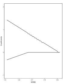
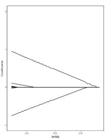
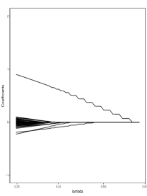
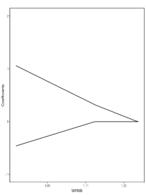
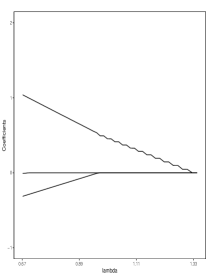
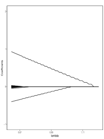
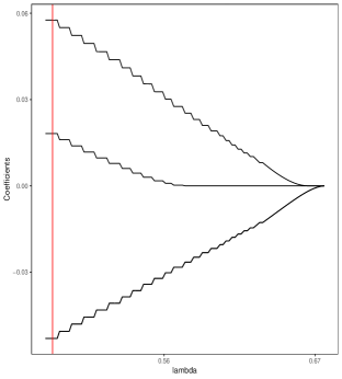
Figure 1 shows the solution paths of the symmetric estimation for the sparse case and the asymptotic sparse case with different data dimension . We can see that the penalized methods (2.5) does can recover the support of the differential network when the tuning parameter is suitably chosen.
 (A):
(B):
(C):
 (D):
(E):
(F):
4 Real Data Analysis
In this section we apply our algorithm to two real data sets.
4.1 Spambase Data Set
In this example, we model the differential network of spam and non-spam emails. The data is publicly available at https://archive.ics.uci.edu/ml/datasets/spambase, which includes 1813 spam emails and 2788 non-spam emails. The data set collects 56 attributes including the frequency of the words and the characters and also the length of the uninterrupted sequences of capital letters. More details can be found in the website.
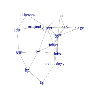
We standardize the data and use a non-paranormal transformation to relax the assumption of Gaussian distribution. Figure (2) illustrates the estimator given by our algorithm, where each node represents a specific feature. Our method indicates the existence of several hub features, including “direct”, “telnet”, “technology”, “labs” and “hp”. Therefore, there might exist covariance structure changes between spam and non-span emails. For example, since the data is donated by Hewlett-Packard Labs, the words “telnet”, “hp” and “technology” will have a higher frequency in non-spam emails which means these features can help researchers to label the emails.
4.2 Hepatocellular Carcinoma Data Set
As a second example, we apply our algorithm to mRNA expression data of liver cancer patients from International Cancer Genome Consortium which is available at https://icgc.org/icgc/cgp/66/420/824. Several pathways from the KEGG pathway database (Ogata et al., 1999; Kanehisa et al., 2012) were studied to determine the conditional dependency relationships between liver cancers and normal patterns.
To deal with the original data, we perform three steps. Firstly, we constrain the mRNAs in the following pathway: Pathways in cancer(05200), Transcriptional misregulation in cancer(05202), Viral carcinogenesis(05203), Chemical carcinogenesis(05204), Proteoglycans in cancer(05205), MicroRNAs in cancer(05206), Central carbon metabolism in cancer(05230), Choline metabolism in cancer(05231), and Hepatocellular carcinoma(05225). Secondly, we use the impute function from the R impute package to fill out the missing values. Thirdly, we standardize the data and use a non-paranormal transformation. This left us with 223 liver cancer patients and 222 normal patients with 1209 mRNAs in all.
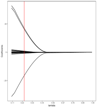
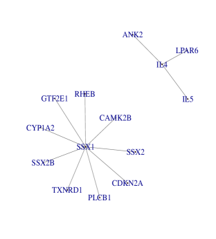
Figure (3) summarizes the estimation given by our algorithm, where each node represents a specific mRNA. This figure show that real transcription networks often contain hub nodes. Our method indicates that SSX1 is an important mRNA. Indeed, SSX1 is a valid treatment option for CTNNB1 mutation positive HCC patients, while CTNNB1 is one of major mutations. Moreover, SSX1 as an oncogene is functionally validated (Ding et al., 2014).
Acknowledgments
Yu is supported in part by 2016YFC0902403 of Chinese Ministry of Science and Technology, and by National Natural Science Foundation of China 11671256. Wang is partially supported by Shanghai Sailing Program 16YF1405700 and National Natural Science Foundation of China 11701367.
Appendix
By the main results of Beck and Teboulle (2009), to complete the proof of the Theorem 1, we only need to show that the loss function is convex which is the results of the following lemma.
Lemma 4.1
The loss function (2.3) is a smooth convex function, and its gradient is Lipschitz continuous with Lipschitz constant , that is
where is the largest eigenvalue of the sample covariance matrix for .
Proof: Since the loss function (2.3) is defined by
we can calculate the gradient of
and the Hessian matrix is . Since both covariance matrices and are definite positive matrix, the Hessian matrix is a definite positive matrix. Hence, the loss function is a smooth convex function.
Moreover, for any , we have
The proof is now completed.
References
- Anderson (2003) T. Anderson. An introduction to multivariate statistical analysis, 2003.
- Bandyopadhyay et al. (2010) S. Bandyopadhyay, M. Mehta, D. Kuo, M.-K. Sung, R. Chuang, E. J. Jaehnig, B. Bodenmiller, K. Licon, W. Copeland, M. Shales, et al. Rewiring of genetic networks in response to DNA damage. Science, 330(6009):1385–1389, 2010.
- Barabási and Oltvai (2004) A.-L. Barabási and Z. N. Oltvai. Network biology: understanding the cell’s functional organization. Nature Reviews Genetics, 5(2):101, 2004.
- Barabási et al. (2011) A.-L. Barabási, N. Gulbahce, and J. Loscalzo. Network medicine: a network-based approach to human disease. Nature Reviews Genetics, 12(1):56, 2011.
- Beck and Teboulle (2009) A. Beck and M. Teboulle. A fast iterative shrinkage-thresholding algorithm for linear inverse problems. SIAM Journal on Imaging Sciences, 2(1):183–202, 2009.
- Bickel and Levina (2008) P. J. Bickel and E. Levina. Regularized estimation of large covariance matrices. Annals of Statistics, 36(1):199–227, 2008.
- Boyd et al. (2011) S. Boyd, N. Parikh, E. Chu, B. Peleato, and J. Eckstein. Distributed optimization and statistical learning via the alternating direction method of multipliers. Foundations and Trends® in Machine Learning, 3(1):1–122, 2011.
- Cai and Liu (2011) T. Cai and W. Liu. Adaptive thresholding for sparse covariance matrix estimation. Journal of the American Statistical Association, 106(494):672–684, 2011.
- Cai et al. (2011) T. Cai, W. Liu, and X. Luo. A constrained minimization approach to sparse precision matrix estimation. Journal of the American Statistical Association, 106(494):594–607, 2011.
- Ding et al. (2014) X. Ding, Y. Yang, B. Han, C. Du, N. Xu, H. Huang, T. Cai, A. Zhang, Z.-G. Han, W. Zhou, and L. Chen. Transcriptomic characterization of hepatocellular carcinoma with ctnnb1 mutation. PLoS One, 9(5), 2014.
- Fan et al. (2016) J. Fan, Y. Liao, and H. Liu. An overview of the estimation of large covariance and precision matrices. The Econometrics Journal, 19(1):C1–C32, 2016.
- Gambardella et al. (2013) G. Gambardella, M. N. Moretti, R. De Cegli, L. Cardone, A. Peron, and D. Di Bernardo. Differential network analysis for the identification of condition-specific pathway activity and regulation. Bioinformatics, 29(14):1776–1785, 2013.
- Jerome et al. (2008) F. Jerome, H. Trevor, and T. Robert. Sparse inverse covariance estimation with the graphical lasso. Biostatistics, 9(3):432–441, 2008.
- Jian et al. (2011) G. Jian, L. Elizaveta, M. George, and Z. Ji. Joint estimation of multiple graphical models. Biometrika, 98(1):1–15, 2011.
- Jiang et al. (2018) B. Jiang, X. Wang, and C. Leng. A direct approach for sparse quadratic discriminant analysis. Journal of Machine Learning Research, 19(31):1–37, 2018.
- Julien et al. (2011) C. Julien, G. Yves, and A. Christophe. Inferring multiple graphical structure. Statistics and Computing, 21(4):537–553, 2011.
- Li and Shao (2015) Q. Li and J. Shao. Sparse quadratic discriminant analysis for high dimensional data. Statistica Sinica, 25:457–473, 2015.
- Meinshausen and Bühlmann (2006) N. Meinshausen and P. Bühlmann. High-dimensional graphs and variable selection with the lasso. Annals of Statistics, 34(3):1436–1462, 2006.
- Nesterov (1983) Y. Nesterov. A method for solving the convex programming problem with convergence rate . Soviet Math Dokl, 27:372–376, 1983.
- Rothman et al. (2009) A. J. Rothman, E. Levina, and J. Zhu. Generalized thresholding of large covariance matrices. Journal of the American Statistical Association, 104(485):177–186, 2009.
- Tibshirani (1996) R. Tibshirani. Regression shrinkage and selection via the lasso. Journal of the Royal Statistical Society, Series B, 58(1):267–288, 1996.
- Tong et al. (2014) T. Tong, C. Wang, and Y. Wang. Estimation of variances and covariances for high-dimensional data: a selective review. Wiley Interdisciplinary Reviews: Computational Statistics, 6(4):255–264, 2014.
- Yuan et al. (2017) H. Yuan, R. Xi, C. Chen, and M. Deng. Differential network analysis via the lasso penalized D-trace loss. Biometrika, 104(4):755–770, 2017.
- Zhang and Zou (2014) T. Zhang and H. Zou. Sparse precision matrix estimation via lasso penalized D-trace loss. Biometrika, 101(1):103––120, 2014.
- Zhao et al. (2014) S. D. Zhao, T. T. Cai, and H. Li. Direct estimation of differential networks. Biometrika, 101(2):253–268, 2014.
- Zhu and Li (2018) Y. Zhu and L. Li. Multiple matrix gaussian graphs estimation. Journal of the Royal Statistical Society, Series B, 2018.