Lagrangian stability of the Malvinas Current

Abstract

Deterministic and probabilistic tools from nonlinear dynamics are used to assess enduring near-surface Lagrangian aspects of the Malvinas Current. The deterministic tools are applied on a multi-year record of velocities derived from satellite altimetry data, revealing a resilient cross-stream transport barrier. This is composed of shearless-parabolic Lagrangian coherent structures (LCS), which, extracted over sliding time windows along the multi-year altimetry-derived velocity record, lie in near coincidental position. The probabilistic tools are applied on a large collection of historical satellite-tracked drifter trajectories, revealing weakly communicating flow regions on either side of the altimetry-derived barrier. Shearless-parabolic LCS are detected for the first time from altimetry data, and their significance is supported on satellite-derived ocean color data, which reveal shapes that quite closely resemble the peculiar V shapes, dubbed “chevrons,” that have recently confirmed the presence of similar LCS in the atmosphere of Jupiter. Finally, using in-situ velocity and hydrographic data, conditions for symmetric stability are found to be satisfied, suggesting a duality between Lagrangian and Eulerian stability for the Malvinas Current.

The Malvinas Current originates as a result of a pronounced northward turn of the northern edge of the Antarctic Circumpolar Current past the Drake Passage. Carrying within a substantial portion of the upper limb of the Atlantic Meridional Overturning Circulation [1], it represents a northward pathway for nutrient-rich subpolar water, making the western margin of the Argentine Basin a region of enhanced biological activity [2] and significant fisheries [3]. The Malvinas Current flows northward up to about 38^∘S, where it sharply turns eastward upon meeting the southward-flowing Brazil Current to form the Brazil–Malvinas Confluence [4], a region characterized by high mesoscale variability [5]. Lagrangian observations have suggested that the Malvinas Current is composed of a single barotropic jet extending down to 750-m depth or more for most of its northward path along the western boundary [6] as is constrained by potential vorticity conservation [7, 8]. High-resolution hydrographic data and direct current observations more recently suggested the presence multiple baroclinic jets in addition to the main barotropic one [9], confirming earlier inferences made from the analysis of the surface thermal structure [10].

The analysis of the surface thermal structure more specifically revealed regions of large temperature contrast along cores of high meridional velocity [9]. This finding is consistent with the expectation that the Malvinas Current should behave as barrier for cross-stream transport. This expectation is motivated by behavior of jetstreams in the lower stratosphere [11, 12, 13, 14, 15] and the weather layer of Jupiter [16, 17] as well as earlier speculation that western boundary currents such as the Gulf Stream should behave as transport barriers [18] and more recent work that has characterized zonal ocean currents as cross-stream mixing inhibitors [19], which has been partially verified by applying heuristic analyses involving satellite altimetry data, drifter trajectories, and ocean color imagery [20, 21, 22, 23]. Our goal in this paper is to test the above expectation and further assess its persistence over time.

To achieve our goal we use two types of tools from nonlinear dynamics, both especially designed to investigate global aspects of Lagrangian motion. One set of tools is deterministic, and build on geometric, observer-independent (or objective) notions of strain and shear. They target so-called Lagrangian coherent structures (LCS) [24] as organizers of the Lagrangian circulation. This is done by means of a collection of global variational principles that constitute the geodesic theory of LCS [25, 26, 27, 28, 29, 30, 31, 32, 33]. The deterministic tools are more effective when the velocity field is known as this can be integrated to generate the required flow map that needs to be subsequently differentiated with respect to initial positions.

The other set of tools considered is probabilistic. These tools root in ergodic theory and, under appropriate time-homogeneity assumptions, can unveil from the Lagrangian circulation statistically weak communicating flow regions that form the basis for the construction of Lagrangian geographies [34, 35, 36, 37]. The theoretical foundation for this is provided by a series of results from the study of autonomous dynamical systems using probability densities that have led to the notion of almost-invariant sets [38, 39, 40, 41, 42]. Central to this approach is the Perron–Frobenius (or transfer) operator [43] and the transition matrix, its discrete version that defines a Markov chain [44, 45, 46] on boxes covering the flow domain. The probabilistic tools do not require flow map differentiation and can be applied directly on Lagrangian trajectories that do not start simultaneously under the above assumptions.

The deterministic tools are applied on a multi-year record of velocities derived from satellite altimetry data, revealing a persisting cross-stream transport barrier associated with the Malvinas Current in the near surface ocean. This barrier is composed of shearless-parabolic LCS, which, extracted over sliding time windows along the multi-year altimetry-derived velocity record, lie in near-coincidental position. Shearless-parabolic LCS generalize the concept of twistless invariant KAM (Kolmogorov–Arnold–Moser) tori from time-periodic [47, 48] or quasiperiodic [49, 12] flows to finite-time-aperiodic flows. The probabilistic tools are applied on a large collection of historical satellite-tracked trajectories of drifters drogued at 15 m, revealing statistically weak communicating flow regions on either side of the altimetry-derived barrier.

Shearless-parabolic LCS are detected for the first time from altimetry data, and their significance is supported on satellite-derived ocean color data. Patterns revealed in such data are found to organize into V shapes nearly axially straddling the altimetry-derived LCS consistent with their shearless-parabolic nature [30]. Such V shapes have been to the best of our knowledge only reported to develop by clouds in the atmosphere of Jupiter at the boundaries of its characteristic zonal strips [50]. The significance of the enduring cross-stream transport barrier which characterizes the Malvinas Current is independently supported on drifter data. Furthermore, in-situ velocity and hydrographic data are used to suggest a duality between Lagrangian and Eulerian stability for the current.

The rest of the paper follows the standard organization into a methods section, a results section, and a summary and conclusions section. The various types of data considered are described as they are employed. Finally, the online Supplementary Information provides additional details on the deterministic and probabilistic tools as well as on the Eulerian stability result considered, thereby making the paper quite selfcontained.

Methods

Deterministic tools.

The deterministic procedure involved in shearless-parabolic LCS extraction is succinctly as follows (cf. Section A in the online Supplementary Information for an expanded discussion). Given an incompressible, two-dimensional velocity field $v(x,t)$, the fluid trajectory equation

$$\dot{x}=v(x,t)$$ (1)

is integrated over the time interval $[t_{0},t]$ to form the Cauchy–Green tensor

$$C_{t_{0}}^{t}(x_{0})=\operatorname{D}\!{F}_{t_{0}}^{t}(x_{0})^{\top}\operatorname{D}\!{F}_{t_{0}}^{t}(x_{0}),$$ (2)

where $F_{t_{0}}^{t}$ is the flow map that takes initial positions $x_{0}$ at $t_{0}$ to positions $x(t;x_{0},t_{0})$ at $t$. The eigenvalues and eigenvectors of this observer-independent (i.e., objective) measure of deformation, satisfying

$$0<\lambda_{1}(x_{0})\equiv\lambda_{2}(x_{0})^{-1}\leq 1,\quad\xi_{1}(x_{0})\perp\xi_{2}(x_{0}),$$ (3)

are then computed.

Time-$t_{0}$ positions of shearless-parabolic LCS are subsequently sought as material lines formed by chains of alternating segments of Cauchy–Green tensorlines everywhere tangent to $\xi_{1}(x_{0})$ and $\xi_{2}(x_{0})$, namely, curves $r(s)$ satisfying

$$r^{\prime}=\xi_{i}(r),\quad i=1,2.$$ (4)

The $\xi_{1}(x_{0})$- and $\xi_{2}(x_{0})$-line segments are chosen:

1. to connect wedge and trisector singularities where $C_{t_{0}}^{t}(x_{0})=\operatorname{Id}$, so the construction is structurally stable (i.e., robust under flow map perturbations); and

2. such that $\smash{\sqrt{\lambda_{1}(x_{0})}}\approx 1$ and $\smash{\sqrt{\lambda_{2}(x_{0})}}\approx 1$, respectively, so along-segment squeezing and stretching is kept close to neutral, thereby minimizing their hyperbolic nature.

A disk filled with tracer which is initially divided into two halves by one such shearless-parabolic LCS will, therefore, deform into a V shape axially straddling the LCS [30]. Observation of such behavior represents a more stringent test of the presence of a shearless-parabolic LCS with a cross-stream transport inhibitor effect than the observation of a large tracer contrast, which can be produced by LCS of any type.

Probabilistic tools.

Central to the probabilistic approach is a transition matrix $P\in\mathbb{R}^{N\times N}$ with components (cf. Section B in the online Supplementary Information for details)

$$P_{ij}:=\operatorname{\mathrm{Pr}}[\xi_{t+\mathcal{T}}\in B_{j}\mid\xi_{t}\in B_{i}]$$ (5)

for a given transition time $\mathcal{T}$ and any time $t$, which provides a discrete representation of a transfer operator for the passive evolution on a domain $X$ of tracers governed by a time-homogeneous advection–diffusion process. Drawn from a uniform distribution on $B_{i}$, $\xi_{t}$ is the initial position of a discrete-time trajectory $\{\xi_{t},\xi_{t+\mathcal{T}},\xi_{t+2\mathcal{T}},\dotsc\}$ described by a tracer particle that randomly jumps, according to the stochastic kernel of the advection–diffusion process, between boxes in a collection $\smash{\{B_{1},\dotsc,B_{N}\}}$ covering $X$. If $X$ is closed, then $\smash{\sum_{j=1}^{N}}P_{ij}=1$ for every $i$, i.e., $P$ is row-stochastic. By construction, $P$ defines a Markov chain with states represented by the boxes of the partition. The discrete representation of a tracer probability density $f(x)$, i.e., satisfying $\smash{\int_{X}}f(x)\operatorname{d}\!{x}=1$, is a probability vector $\mathbf{f}=(f_{1},\cdots,f_{N})$, where $f_{i}=\int_{B_{i}}f(x)\operatorname{d}\!{x}$ so $\smash{\sum_{i=1}^{N}}f_{i}=1$. This evolves $k\mathcal{T}$ units of time according to

$$\mathbf{f}^{(k)}=\mathbf{f}P^{k},\quad k=1,2,\dotsc.$$ (6)

Long-time asymptotic aspects of the evolution on the Markov chain described $P$ can be inferred from its spectral properties [51, 39, 41] as follows.

If $P$ is irreducible (i.e., all states in the Markov chain communicate) and aperiodic (i.e., no state is revisited cyclically), its dominant left eigenvector, $\mathbf{p}$, satisfies $\mathbf{p}P=\mathbf{p}$, can be chosen (componentwise) positive, and (scaled appropriately) represents a limiting invariant distribution, namely, $\mathbf{p}=\smash{\lim_{k\uparrow\infty}\mathbf{f}P^{k}}$ for any probability vector $\mathbf{f}$ (cf., e.g., Horn and Johnson [45]). In particular, $\mathbf{f}=\mathbf{1}/N$, where $\mathbf{1}=P\mathbf{1}$ is the right eigenvector corresponding to $\mathbf{p}$.

The left eigenvector of $P$ with $\lambda$ closest to 1, $\mathbf{l}_{2}$, is a signed vector which decays at the slowest rate [52, 53]. Sets where the magnitude of the components of $\mathbf{l}_{2}$ maximize are the most dynamically disconnected as a random walker starting there will take the longest time to transit to other sets. The corresponding right eigenvector, $\mathbf{r}_{2}$, is also a signed vector, but it typically includes well-defined plateaus. A random trajectory conditioned on starting in a set forming the support of a plateau is expected to distribute in the long run, albeit only temporarily, as $\mathbf{l}_{2}$ where it takes a single like sign [54, 34]. Such sets are therefore expected to form basins of attraction for time-asymptotic almost-invariant sets.

Decomposition of the ocean flow into weakly disjoint basins of attraction for almost-invariant attractors using the above spectral method has been shown to form the basis of a Lagrangian geography of the ocean, where the boundaries between basins are determined from the Lagrangian circulation itself, rather than from arbitrary geographical divisions [34, 35, 36]. The number of Lagrangian provinces will depend on the number of right eigenvectors considered. A large gap in the eigenspectrum of $P$ provides a cutoff criterion for eigenvector analysis, as provinces extracted from eigenvectors with eigenvalues on the right of the gap will have significantly shorter retention times than those extracted from eigenvectors on the left.

Results

Deterministic analysis.

The deterministic tools are applied on a velocity field derived from sea-surface height (SSH) in the region of interest, spanning $[70^{\circ}\text{W},50^{\circ}\text{W}]\times[55^{\circ}\text{S},30^{\circ}\text{S}]$. Specifically, we consider

$$v(x,t)=gf^{-1}\nabla^{\perp}\eta(x,t)$$ (7)

where $g$ is gravity, $f$ is the mean Coriolis parameter, and $\eta(x,t)$ is the superimposition on a mean dynamic topography [55] of a daily $0.25^{\circ}$-resolution SSH anomaly field constructed from along-track satellite altimetry measurements [56]. Such an altimetry-derived velocity reflects an integral dynamic effect of the density field near the ocean surface, i.e., above the thermocline [57].

Figure 1 illustrates the application of the deterministic procedure on $t_{0}=\text{12 Dec 2001}$ with $T=t-t_{0}=-15$ days, which was kept fixed throughout. Here and in the calculations that we describe below, the integration of trajectories (1) and tensorlines (4) are carried out using a stepsize-adapting fourth-order Runge–Kutta method. Unlike trajectory integration, tensorline integration involves stepwise orienting the eigenvector field(s). Interpolations are obtained using a cubic scheme. Flow map differentiation in (2) is performed using finite differences. The Lagrangian coherence horizon $|T|=15$ days was selected such that sufficiently long shearless-parabolic LCS can be extracted. Long LCS impact transport more effectively than short LCS, which tend to coexist with a much longer LCS for this $|T|$ choice and thus are ignored. As $|T|$ is increased, singularities of the Cauchy–Green tensor tend to proliferate, resulting typically only in very short shearless-parabolic LCS with small effect on transport. The (time) integration direction, in turn, has been conveniently adopted to enable comparison with observed (e.g., satellite-derived) tracer distributions. More specifically, a tracer distribution at any given time is the result of the action of the flow on the tracer up to that time.

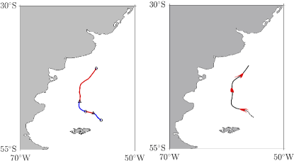
Figure 1: (left) Shearless-parabolic LCS extracted from altimetry-derived velocity on $t_{0}=\text{12 Dec 2001}$ using backward integration with $T=-15$ days. Portions of the LCS colored red and blue are nearly neutral squeezing and stretching tensorline segments of the Cauchy–Green tensor field, respectively, connecting wedge and trisector singularities of the field, indicated by triangles and circles, respectively. (right) Forward-advected images at $t_{0}$ of circles axially straddling the backward-advected image of the LCS at $t_{0}-|T|$.

Depicted in the left panel of Fig. 1 is the longest shearless-parabolic LCS found in the domain. The nearly neutral squeezing and stretching Cauchy–Green tensorline segments that form the LCS are shown in blue and red, respectively. The wedge and trisector singularities connected by these segments are indicated by triangles and circles, respectively. The shearless-parabolic nature of the extracted LCS is demonstrated in the right panel of Fig. 1, which shows the forward-advected image at time $t_{0}$ of three tracer disks axially straddling the backward-advected image of the LCS at $t_{0}-|T|$. Note that the disks deform, as expected, into V shapes which very closely axially straddle the LCS at $t_{0}$.

Figure 2 shows a satellite-derived ocean pseudo-true color image on $t_{0}=\text{12 Dec 2001}$ with the extracted shearless-parabolic LCS overlaid. The coloration in the image is determined by the interactions of incident light with particles present in the water, mainly pigment chlorophyll, sediments, and dissolved organic material. Thus patterns formed in an ocean color image can be thought, to first approximation, as developed by a passive tracer. Note the various V-shaped patches nearly axially straddling the extracted LCS. This provides strong independent observational support for the altimetry-inferred LCS and its shear-parabolic nature. Ocean color images showing V shapes of the type reported here are very rare; to the best of our knowledge we report their occurrence for the first time. Analogous V shapes, dubbed “chevrons,” have been relatively recently observed in cloud distributions in the weather layer of Jupiter at the boundaries between so-called belts and zones organized around zonal jets [50]. Jovian zonal jets have been rigorously characterized as shear-parabolic LCS [17] and earlier heuristically as twistless KAM tori [16].

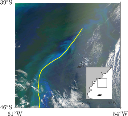
Figure 2: Ocean pseudo color image on 12 Dec 2001 derived from the Moderate Resolution Imaging Spectroradiometer (MODIS) aboard Terra with the shearless-parabolic LCS extracted from altimetry overlaid.

Shearless-parabolic LCS extraction was applied on sliding time windows $[t_{0}-|T|,t_{0}]$ with $t_{0}$ selected every two weeks since 15 Oct 2002 until 15 Sep 2005. During the period chosen, altimetry measurements were made by altimeters mounted on four satellites, thereby maximizing their availability and thus the quality of the derived velocity [58, 59].

The extracted shearless-parabolic LCS are depicted (in red) in Fig. 3 along with mean (over the LCS extraction period, 15 Oct 2002–15 Sep 2005) streamlines of the altimetry-derived flow. The latter were selected to fill a strip around the Eulerian axis of the Malvinas Current, here taken as the streamline where the mean velocity maximizes at 42^∘S. Note that LCS and streamlines do not coincide in position. Yet they run close inside the latitudinal band between about 38 and 49^∘S. This suggests that the Malvinas Current behaves, within that latitudinal band, as a quasi-steady shearless-parabolic LCS. As such, it inhibits cross-stream transport persistently over time, largely preventing Patagonian shelf water from mixing with off-shelf water. The rather tightly packed collection of LCS forms the Lagrangian axis (or, more accurately, core) of the current.

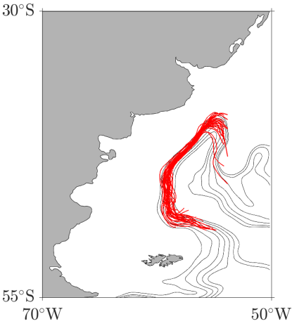
Figure 3: Mean (15 Oct 2002–15 Sep 2005) streamlines along the Malvinas current core (black) overlaid with shearless-parabolic LCS extracted over windows $[t_{0}+T,t_{0}]$ with $t_{0}$ sliding monthly over 30 Oct 2002–15 Sep 2005 and $T=-15$ days.

The cross-stream barrier nature of the Malvinas Current is verified explicitly by the ensemble-mean evolution of tracers under the altimetry-derived flow. Selected snapshots are shown in Fig. 4. The ensemble-mean tracer evolution was computed by evolving the tracers from the same initial location on the shelf northeast of the Malvinas Islands, every two months over 15 Oct 2002–15 Sep 2005, and then computing on a daily basis during roughly half a year the percentage of tracer particles visiting each 0.75^∘-side box of a grid covering the domain. Note that the ensemble-mean tracer transport across the LCS is negligible.

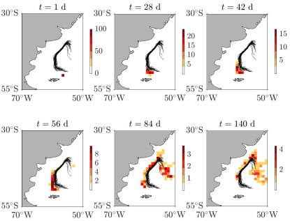
Figure 4: Snapshots of the ensemble-mean evolution over 15 Oct 2002–15 Sep 2005 of tracers under the altimetry-derived flow with the extracted shearless-parabolic LCS overlaid. The percentage of tracer particles visiting the boxes of a grid covering the domain is shown.

Practically all of the transport off the shelf takes place near 38^∘S, where the collection of extracted shearless-parabolic LCS are interrupted, prior most of them turn very briefly eastward and a few prolong a bit longer southeastward. The transport is directed eastward and then mainly southeastward, out of the domain through two exit routes, one at about 40^∘S and another one at 47^∘S or so. It is important to realize that this is not obvious from the inspection of the mean streamlines, which suggest mainly eastward transport for a tracer released on the shelf at 38^∘S, latitude at about which the Malvinas Current encounters the Brazil Current [4].

The close proximity of the shearless-parabolic LCS and the mean streamlines within 38 and 49^∘S suggests KAM-like behavior. In that latitudinal band, a decomposition of the flow into a steady (reference) component and a small unsteady (perturbation) component, certainly much smaller than near 38^∘S where mesoscale activity is known to be rather strong [5], may be envisioned as in earlier work [60], in principle enabling a near-integrable Hamiltonian system stability analysis [61]. However, the flow is not recurrent, neither in time nor in space. In addition, quite unlike KAM curves, only portions of the reference Hamiltonian level sets (mean streamlines) are seen to “survive” under perturbation (i.e., when motion is produced by the total flow). These important differences indicate that ocean jets can sustain robust barriers for transport far beyond theoretical expectation [49].

Probabilistic analysis.

The probabilistic tools are applied on daily interpolated trajectories produced by satellite-tracked drifting buoys from the NOAA Global Drifter Program [62] that have sampled the domain of interest. The drifter positions are satellite-tracked by the Argos system or GPS (Global Positioning System). The drifters follow the SVP (Surface Velocity Program) design, consisting of a surface spherical float which is drogued at 15 m, to minimize wind slippage and wave-induced drift [63]. The drogue may not be present for the whole extent of a trajectory record [64, 65]. We only consider trajectory portions during which the drogue is present, so a comparison with the altimetry-based results can be attempted.

We first cover the domain by 0.5^∘-side boxes. The size of the boxes was selected to maximize the grid’s resolution while each individual box is sampled by enough drifters. There are on average 28 drifters per box independent of the day over 1993–2013. The $(i,j)$th component of the transition matrix $P$ in (5) is estimated by counting the number of drifters which, visiting at any time $t$ box $B_{i}$, enter box $B_{j}$ at $t+\mathcal{T}$, and then dividing by the number of drifters in $B_{i}$.

Figure 5: (top) A portion of the discrete eigenspectrum of the drifter-based transition matrix $P$ showing the top 15 real eigenvalues. (middle) Left and right ($\mathbf{r}_{2}$) eigenvectors of $P$ with largest none unity eigenvalue ($\lambda_{2}=0.9946$). (bottom) Probability of a trajectory to be retained within regions where $\mathbf{r}_{2}<c$ if $c<0$ or $\mathbf{r}_{2}>c$ if $c>0$ conditioned on starting in those regions.

We have set $\mathcal{T}=2$ days. This in general guarantees interbox communication. Furthermore, $\mathcal{T}=2$ days is longer than the Lagrangian decorrelation timescale, which has been estimated to be of about 1 day [66]. Markovian dynamics can be expected to approximately hold as there is negligible memory farther than 2 days into the past. A similar reasoning was applied in earlier applications involving drifter data [67, 68, 35, 69, 36, 37]. Here the validity of the Markov model was estimated by checking that $\lambda(P(n\mathcal{T}))=\lambda(P(\mathcal{T}))^{n}$ holds well with $n$ up to 5 and consistent with this we have verified that the results presented below are largely insensitive to variations of $\mathcal{T}$ in the range 2–10 days.

We note that while the domain is open, $P$ has been constructed in such a way that it is row-stochastic by excluding all drifter trajectory pieces, which, starting inside the domain, terminate outside. It must be emphasized that this does not force trajectories to spuriously bounce back into the domain. The signature of inward motion is imprinted in the drifter trajectory data, so is in the resulting Markov-chain model. On the other hand, working with a row-stochastic $P$ facilitates the interpretation of the probabilistic tool results, albeit clearly not without exerting some care. Applying the Tarjan algorithm [70] on the directed graph associated with the corresponding Markov chain reveals the existence of a set of boxes in the southwestern corner of the domain that are not reachable from boxes in its complement. The constructed $P$ is thus reducible. Nevertheless, the complement of that set of boxes covers most of the domain and furthermore is absorbing. So excluding it to make $P$ irreducible is inconsequential.

With the above in mind, we show in the top panel of Fig. 5 a portion of the eigenspectrum of $P$ corresponding to the largest 10 real eigenvalues. The largest eigenvalue equals unity and is simple. Consequently, the associated left eigenvector, which we loosely refer to as $\mathbf{p}$, is invariant, yet it is not strictly positive. The right eigenvector is $\mathbf{1}$. Any probability vector forward evolves under left multiplication by $P$ into $\mathbf{p}$, whose components maximize along the eastern boundary of the domain. More specifically, this happens inside the regions delimited by the black curves in the middle-left panel of Fig. 5. A tracer, irrespective of how it is initialized in the domain, will thus in the long run accumulate in those regions of the eastern boundary. Physically this means that it will eventually exit the domain through those locations. Once the tracer gets attracted there (exists the domain) it will not recirculate back into the domain.

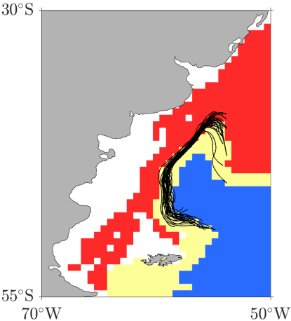
Figure 6: Lagrangian geography deduced from the structure of the dominant right eigenvector of the drifter-based transition matrix $P$ overlaid with all shearless-parabolic LCS extracted from satellite altimetry. Retention probability and time are maximized in the red and blue provinces, which represent the main Lagrangian provinces, while the yellow province represents a transition region with smaller retention probability and time (cf. Table 1).

The middle panel of Fig. 5 shows the left ($\mathbf{l}_{2}$) and right ($\mathbf{r}_{2}$) eigenvectors of $P$ corresponding to the second eigenvalue closest to 1 ($\lambda_{2}=0.9934$). Note the two regions where the magnitude of the components $\mathbf{l}_{2}$ maximize. The support of these small regions represent almost-invariant attracting sets for tracers initially distributed on the large regions where $\mathbf{r}_{2}$ takes constant values, which represent their basins of attraction. (The eigenvectors have been arbitrary assigned sings such that regions of $\mathbf{r}_{2}$ evolve to like signed regions of $\mathbf{l}_{2}$.) These almost-invariant attracting sets, centered at about 38.5 and 48^∘S at the eastern side of the domain, physically represent routes of escape out of the domain for tracers in the corresponding basins of attraction. Traces initially inside each basin will passively evolve toward the respective attractor, which, being almost invariant, will retain the tracers temporarily until they are eventually drained out of the domain. Thus while $\mathbf{p}$ indicates that tracers will eventually exit the domain through the eastern boundary, $\mathbf{l}_{2}$ reveals preferred exit paths depending on how they are initialized.

The eigenspectrum of $P$ in the portion shown in the top panel of Fig. 5 reveals a gap between $\lambda_{2}$ and $\lambda_{3}$. Indeed, there is a drop of 2.1702% from $\lambda_{2}$ to $\lambda_{3}$, while $\lambda_{1}$ and $\lambda_{2}$ only differ by 0.0066% and $\lambda_{3}$ through $\lambda_{5}$ are very similar, changing by just 0.0091% on average. This suggests that a minimal significant Lagrangian geography with sufficiently large weakly communicating provinces to substantively constrain connectivity in the domain can be constructed by inspecting $\mathbf{r}_{2}$. A geography composed of smaller and less isolated provinces may be obtained by inspecting additional right eigenvectors, but this is not pursued here as our interest is to independently verify the deterministic analysis of the altimetry data, which suggested weak communication between shelf water on the west of the Malvinas Current and the open-ocean water on the east.

	red	yellow	blue
$\rho$	0.9763	0.7797	0.9835
$\tau$	7.7952	1.1518	11.4850

Table 1: Retention probability ($\rho$) and time ($\tau$, in months) inside each of the three provinces of the Lagrangian geography in Fig. 6, which are labelled by their colors in the figure.

Shown in Fig. 6 is the constructed minimal Lagrangian geography. It includes three provinces, which are defined as follows. Rather than defining the Lagrangian provinces as sets where $\mathbf{r}_{2}$ takes one sign, as done in earlier work [34, 35, 36], here we define them as sets where the retention probability is maximized. More specifically, let $\mathcal{A}\subset\{1,\dotsc,N\}$ and define $A:=\smash{\bigcup_{i\in\mathcal{A}}}B_{i}\subset X$. If one conditions on a tracer trajectory to start in set $A$, the probability to be retained within $A$ after one application of $P$ is $\rho(A):=\smash{\sum_{i,j\in\mathcal{A}}}p_{i}P_{ij}/\smash{\sum_{i\in\mathcal{A}}}p_{i}$ [39, 41]. The bottom panel shows $\rho$ for $A(c):=\smash{\bigcup_{i:\mathbf{r}_{2}<c}}B_{i}$ if $c<0$ or $\smash{\bigcup_{i:\mathbf{r}_{2}>c}}B_{i}$ if $c>0$. We compute $\max_{c}\rho(A(c))=0.9835$ and $0.9763$ at at $c=c_{-}=-0.0016$ and $c=c_{+}=0.0219$, respectively. The sets $A_{\text{blue}}:=\smash{\bigcup_{i:\mathbf{r}_{2}<c_{-}}}B_{i}$ and $A_{\text{red}}:=\smash{\bigcup_{i:\mathbf{r}_{2}>c_{+}}}B_{i}$, depicted red and blue in Fig. 6, respectively, form the main Lagrangian provinces. The set depicted yellow, $A_{\text{yellow}}:=\smash{\bigcup_{i:c_{-}<\mathbf{r}_{2}<c_{+}}}B_{i}$, represents a transition province with smaller retention probability, $\rho(A_{\text{yellow}})=0.7797$.

Larger (smaller) retention probability is associated with longer (shorter) retention time. A simple measure of retention time is computed as follows. Consider $\mathbf{p}_{A}P|_{A}=\lambda_{A}\mathbf{p}_{A}$, where $P|_{A}$ is $P$ restricted to some set $A\subset X$ and $\lambda_{A}$ is the largest eigenvalue of $P|_{A}$. If $P$ is irreducible, $\lambda_{A}<1$ and $\mathbf{p}_{A}\geq 0$. Assume that a tracer trajectory starts in $A$. If the trajectory is conditioned on being retained in $A$, it will asymptotically distribute as $\mathbf{p}_{A}$, where $\mathbf{p}_{A}$ has been normalized to a probability vector. Such a $\mathbf{p}_{A}$ is called a quasi-stationary distribution (cf. Chapter 6.1.2 of Bremaud [71]). The expectation of the random time to exit $A$ is $\tau(A):=\mathcal{T}/(1-\lambda_{A})$ (cf. Section B.7 in the online Supplementary Information). Such a $\tau(A)$ provides an average measure of retention time in $A$. We compute $\tau(A_{\text{blue}})=11.5$ months and $\tau(A_{\text{red}})=7.7952$ months for the main Lagrangian provinces, and a much shorter retention time, $\tau(A_{\text{yellow}})=1.1518$ months, for the transition province.

Clearly, the partition of the flow domain provided by the drifter-based Lagrangian geography is indicative of low connectivity between shelf water and open-ocean water off the shelf, south of 38^∘S. Figure 7 provides confirmation for this inference from direct calculation. More specifically, this figure shows selected snapshots of the evolution under left multiplication by $P$ of a tracer probability initially on the shelf, northeast of the Malvinas archipelago. Note that up to day 56, the tracer probability propagates northeastward, predominantly confined within the transition province of the Lagrangian geography. The almost-invariant character of the boundaries of the Lagrangian provinces explains the small leakage of probability over the main provinces east and west of the transition province.

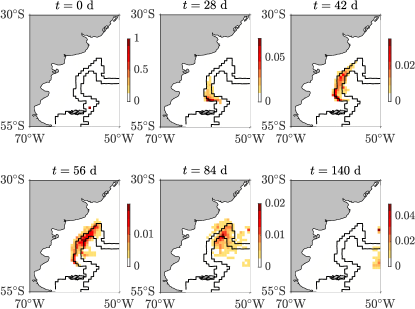
Figure 7: Snapshots of the drifter-based forward evolution of a probability density with the boundaries of the main Lagrangian provinces indicated.

The leakage continues past day 56 of evolution, becoming stronger as the Brazil–Malvinas Confluence near 38^∘s is reached. Time-asymptotically the probability that leaks to the west and east of the transition province accumulates in the southern and northern almost-invariant attractor, respectively (cf. Fig. 5, middle-left panel). These attractors, we reiterate, physically represent exit routes out of the domain.

We note that if the tracer probability were initialized inside the transition province of the Lagrangian geography where this turns (south)eastward at about 38^∘s, it would remain confined within for a shorter period of time before leaking out and being absorbed into the nearest almost-attracting set. The reason for this is the much closer proximity of the attractors to the transition province at these latitudes. The retention time measure $\tau(A_{\text{yellow}})=1.1518$ months, discussed above, is an average measure for the entire transition province. The average retention time within the portion of transition province that lies (roughly) inside the Brazil–Malvinas Confluence region is somewhat smaller than 1 week. By contrast, the average retention time in the complement of this set is nearly 5 weeks, which is very close to the average retention time in the whole transition province. This is consistent with the behavior just described. Also consistent with this is the strong mesoscale variability that affects the area where the Malvinas and Brazil currents meet. Diffusion is benefited from such variability, which contributes to shorten the retention time there.

To assess the latter, one can leverage on the computation of the flux across the boundary of a set $A(=\smash{\bigcup_{i\in\mathcal{A}}}B_{i})$, which is readily accomplished as follows [72]. Let $\partial\mathcal{A}(\subset\mathcal{A})$ be the index set of boxes on the boundary of $A$. The flux $\Phi(B_{j})$ through a boundary box $B_{j}$, with $j\in\partial\mathcal{A}$, can be calculated as $\Phi(B_{j})=\Phi_{\mathrm{out}}(B_{j})-\Phi_{\mathrm{in}}(B_{j})$, where $\Phi_{\mathrm{out}}(B_{j})=\smash{\mathcal{T}^{-1}}\cdot\operatorname{vol}(B_{j})\smash{\sum_{k\in\{1,\dotsc,N\}\setminus\mathcal{A}}}P_{jk}$ and $\Phi_{\mathrm{in}}(B_{j})=\smash{\mathcal{T}^{-1}}\cdot\smash{\sum_{k\in\{1,\dotsc,N\}\setminus\mathcal{A}}}\operatorname{vol}(B_{k})P_{kj}$. Figure 8 shows an evaluation of the flux formulas for the transition province ($A_{\text{yellow}}$), with $\operatorname{vol}(B_{i})$ estimated as $\operatorname{area}(B_{i})\cdot H$ where $H=15$ m is the drogue depth. Note that the flux through the boundary boxes of these sets tend to maximize inward or outward in the Brazil–Malvinas Confluence region.

Figure 8: (top) Drifter-based estimate of the flux across the boundaries of the transition province of the Lagrangian geography. (bottom) The flux shown as a function of arclength (increasing northward) along each boundary. The red (blue) curve corresponds to the boundary with the main province painted red (blue) in Fig. 6.

We note finally that despite the limitation provided by the number of drifters available, particularly over the continental shelf, the inferred Lagrangian provinces are in very good agreement with the biophysical provinces deduced by Longhurst [2] and more recently by Saraceno et al. [73, 74] using two independent methods.

Synthesis of deterministic and probabilistic analyses.

The results of the deterministic analysis of the altimetry data and the probabilistic analysis of the drifter data are largely consistent. They both independently indicate Lagrangian stability for the Malvinas Current, which largely behaves as a barrier that prevents shelf water to its west from being mixed with off-shelf water to its east. This is well demonstrated in Fig. 6, which shows that the shearless-parabolic LCS extracted from altimetry over sliding time windows along the multiyear record analyzed lie well within the transition province between the main Lagrangian provinces constructed from all available drifter data.

The off-shelf transport takes place near 38^∘S, where the Malvinas Current meets the Brazil Current (cf. Figs. 4 and 7). This region is characterized by strong mesoscale variability, which the probabilistic analysis showed to promote diffusion in the region. Consistent with this, the deterministic analysis revealed LCS prolonging only briefly southeastward at the Brazil–Malvinas Confluence latitude, thereby allowing unrestrained exchanges there. According to both the deterministic and probabilistic results, the off-shelf export eventually reaches the South Atlantic’s interior through two routes.

Lagrangian–Eulerian stability duality.

The reported Lagrangian stability of the Malvinas Current motivates the question of its stability in the Eulerian frame. A stability result for a general meandering meridional current with vertical shear is lacking. Yet the stability of a basic flow (steady solution) $V(x,z)$ in thermal-wind balance, where $x$ is cross-stream and $-z$ depth, of the $y$-independent, inviscid, unforced, nonhydrostatic, Boussinesq equations on an $f$ plane is well established [75, 76]. Both sufficient and necessary conditions for the symmetric stability of $V(x,z)$ under arbitrarily large and shaped perturbations are given by $N^{2}/(\partial_{z}V)^{2}>1/(1+\partial_{x}V/f)>0$, where $N^{2}$ is the square of the basic flow’s Brunt–Väisälä frequency. Note that symmetric stability requires both static stability ($N^{2}>0$) as well as inertial stability ($f^{2}+f\partial_{x}V)>0$). Assuming stable stratification, these conditions are equivalent to $fQ>0$, where $Q:=N^{2}(f+\partial_{x}V)-f(\partial_{z}V)^{2}$ is the basic flow’s potential vorticity, which is materially preserved. Clearly, $fQ<0$ is both necessary and sufficient for symmetric instability. This condition includes the necessary condition for instability under infinitesimally small normal-mode perturbations originally derived by Hoskins [77] (cf. Section C in the online Supplementary Information for a review of the results just described).

Using available direct high-resolution velocity measurements and temperature and salinity data collected by RSS Discovery in late December 1992 during WOCE cruise A11 along 45^∘S [78], we proceed to check if the Malvinas Current has any hope to be symmetrically stable. The WOCE-A11 transect lies across the Malvinas Current, which we assume to be represented as an along-stream-symmetric baroclinic parallel flow. The velocity data was collected by a hull mounted acoustic Doppler current profiler (ADCP) in a westward course. A section of meridional (nearly along-stream) velocity is shown in the top-left panel of Fig. 9. The temperature and salinity were obtained from conductivity-temperature-depth (CTD) casts occupied in a returned eastward course; the Brunt–Väisälä frequency, averaged along the section, is shown in the top-right panel Fig. 9. The bottom-left and bottom-right panels of Fig. 9 show along-section-mean $1/(1+\partial_{x}V/f)$ and $N^{2}/(\partial_{z}V)^{2}$, respectively. Note that the symmetric stability conditions are well satisfied on average across the Malvinas Current. This result together with those from the deterministic and probabilistic nonlinear dynamics analysis suggest a Lagrangian–Eulerian stability duality for the current.

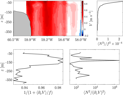
Figure 9: (top left) Meridional velocity section along 45^∘S across the Malvinas Current from a hull mounted ADCP collected on 28 Dec 1992 from RSS Discovery during WOCE cruise A11. (top right) Normalized by the Coriolis parameter squared, along-transect average of Brunt-Väis̈ala frequency squared computed using temperature and salinity from CTD casts during WOCE A11. (bottom left) Along-transect-average of the ratio of the Coriolis parameter and the vertical component of the absolute vorticity. (bottom right) Along-transect-average of Richardson number.

The above result is not obvious whatsoever. Indeed, it is well-known that unsteady laminar Eulerian flows can support irregular Lagrangian motion (chaotic Lagrangian motion generically in bounded, recurrent unsteady two-dimensional flows) [79]. But there are several caveats to have in mind. First, a priori conditions for stability/instability should be verified by the basic flow rather than the total flow and instantaneously as we have checked here. Yet Piola et al. [9] note that the ADCP velocity shear in the 100- through 390-m depth interval is virtually identical to the geostrophic shear derived from hydrography. This suggests that the ADCP velocity may be providing a reasonable representation of the basic velocity. Also, hydrographic data are not available with enough longitudinal resolution to check the symmetric stability conditions pointwise. And last but not least, there are not sufficient data to assess the extent to which along-stream symmetry holds for the Malvinas Current. This has most chances to be verified within 38–49^∘S, (co)incidentally where shearless-parabolic LCS and the mean streamlines were found to lie closest together.

Summary and final remarks

In this paper we have characterized the Malvinas Current as an enduring cross-stream transport barrier by applying nonlinear dynamics tools of two quite different types on independent datasets.

One type of tools used was deterministic, built on a geometric, objective (i.e., observer-independent) notion of material shear. These tools were applied on velocities derived from satellite altimetry, and revealed—for the first time from this dataset—Lagrangian coherent structures (LCS) of the shearless-parabolic class. Computed over sliding time windows along a multiyear period of satellite altimetry data with the highest density, the shearless-parabolic LCS were found to form an enduring near-surface Lagrangian axis for the Malvinas Current that largely inhibits shelf water on its western side from mixing with open-ocean water on its eastern side.

The other type of nonlinear dynamics tools employed was probabilistic, built on ergodic theory and describing tracer motion on a Markov chain. These were applied on available satellite-tracked drifter trajectories, revealing statistically weak communicating Lagrangian provinces separated by the LCS extracted from altimetry. This provided independent support for the enduring role of the Malvinas Current in the near surface as a cross-stream transport barrier.

The shear-parabolic nature of the Lagrangian axis of the Malvinas Current was supported on satellite-derived ocean color imagery. This revealed—for the first time to the best of our knowledge—V shapes nearly axially straddling current’s Lagrangian axis. Similar V shapes, referred to as “chevrons,” have been been relatively recently observed in clouds distributions in the weather layer of Jupiter, confirming the enduring nature of zonal jets there as barriers for meridional transport.

In-situ velocity and hydrographic data showed that conditions for symmetric stability are satisfied. This suggested a Lagrangian–Eulerian stability duality for the Malvinas Current, a nonobvious result given the known ability of laminar Eulerian flows to support irregular Lagrangian motion.

The gas giant’s chevrons have been connected to inertia–gravity wave motion [50]. Satellite imagery has recently revealed internal waves propagating along the Patagonian shelfbreak and continental slope in the opposite direction of the Malvinas Current [80]. The possible connection with the chevrons observed along the Lagrangian axis of the current deserves to be investigated. This is beyond the scope of this paper as also is investigating how representative the results here presented are of other western boundary currents. For instance, high-resolution measurements across the Gulf Stream suggest that symmetric stability is violated locally along submesoscale fronts in the upper ocean [81], which already indicates a potentially important difference with the Malvinas Current.

Author Contributions

FJBV performed the probabilistic dynamical system analysis and the Eulerian stability analysis, and wrote the manuscript; NB carried out the deterministic dynamical system analysis; MS compiled the hydrographic data used in the Eulerian stability analysis; MJO compiled the drifter trajectory data involved in the probabilistic dynamical system analysis; and FJBV, MS, and CS supervised NB’s work. All authors contributed to the interpretation of the results and reviewed the manuscript.

Additional Information

Competing interests: The authors declare no competing interests.

Online Supplementary Information for “Lagrangian stability of the Malvinas Current”

The Supplemtary Information includes three appendices providing additional details on the deterministic (A) and probabilistic (B) tools employed in the paper as well as on the Eulerian stability result considered (C). This is done with a goal in mid of making the paper sufficiently selfcontained.

Appendix A Deterministic tools

A.1 Flow map and Cauchy–Green strain tensor

Consider the motion equation for fluid particles,

$$\dot{x}=v(x,t),$$ (A.1)

where $v(x,t)$ is a two-dimensional incompressible velocity field. Solving this equation for fluid particles at positions $x_{0}$ at time $t_{0}$, one obtains a map that takes the particles to positions $x$ at a later time $t$, namely, $F_{t_{0}}^{t}(x_{0}):=x(t;x_{0},t_{0})$.

A fundamental objective measure of fluid deformation is given by the Cauchy–Green (CG) strain tensor,

$$C_{t_{0}}^{t}(x_{0}):=\operatorname{D}\!{F}_{t_{0}}^{t}(x_{0})^{\top}\operatorname{D}\!{F}_{t_{0}}^{t}(x_{0}).$$ (A.2)

Its eigenvalues and eigenvectors satisfy $0<\lambda_{1}(x_{0})\equiv\lambda_{2}(x_{0})^{-1}\leq 1$ and $\xi_{1}(x_{0})\perp\xi_{2}(x_{0})$, respectively.

A.2 Squeezelines, stretchlines, and singularities

It immediately follows that a well-behaved material curve that at $t_{0}$ is everywhere tangent to $\xi_{1}$ (resp., $\xi_{2}$) will pointwise squeeze (resp., stretch) over $[t_{0},t]$ by $|\operatorname{D}\!{F}_{t_{0}}^{t}(x_{0})\xi_{1}(x_{0})|=\smash{\sqrt{\lambda_{1}(x_{0})}}<1$ (resp., $|\operatorname{D}\!{F}_{t_{0}}^{t}(x_{0})\xi_{2}(x_{0})|$ $=\smash{\sqrt{\lambda_{2}(x_{0})}}>1$).

Good behavior of such squeezelines and stretchlines, i.e., solution curves $s\mapsto r(s)$ to

$$r^{\prime}=\xi_{i}(r),\quad i=1,2,$$ (A.3)

is guaranteed away from singular points $x_{*}$ where the CG tensor is isotropic. Singular points $x_{*}$ are such that $\lambda_{1}(x_{*})=\lambda_{2}(x_{*})$ (or, equivalently in the incompressible case, $C_{t_{0}}^{t}(x_{*})=\operatorname{Id}$) and thus $\xi_{1}(x_{*})$ and $\xi_{2}(x_{*})$ take arbitrary orientations.

Singularities of planar eigenvector fields are analogous to stationary points of planar vector fields [82, 83]. Unlike vector fields, eigenvector fields are bidirectional. However, curves tangent to them or tensorlines are well defined (away from singularities) and thus are referred to as line fields. Line fields on the plane admit two types of structurally stable singularities, namely, trisectors and wedges. A trisector singularity has three hyperbolic sectors, where tensorlines lead away from the singularity in both directions. A wedge singularity has a hyperbolic sector and a parabolic sector, where tensorlines lead away in one direction and toward the singularity in the other, possibly reduced to a single tensorline.

A.3 Shearless-parabolic LCS

The geodesic theory for Lagrangian coherent structures (LCS) of shearless-parabolic type, which are the focus here, seeks such LCS as material curves with neighborhoods showing no leading order change in along-curve-averaged Lagrangian shear [30].

The Lagrangian shear is defined as the tangential projection at time $t$ of the advected image under the linearized flow of a unit normal $n_{0}$ to a time-$t_{0}$ material curve at position $x_{0}$, i.e.,

$$\sigma_{t_{0}}^{t}(x_{0};e_{0}):=\langle\operatorname{D}\!{F}_{t_{0}}^{t}(x_{0})n_{0},e_{t}\rangle\equiv\frac{\langle e_{0},D_{t_{0}}^{t}(x_{0})e_{0}\rangle}{\sqrt{\langle e_{0},C_{t_{0}}^{t}(x_{0})e_{0}\rangle}},$$ (A.4)

where $e_{0}\perp n_{0}$, $e_{t}$ is the unit tangent to the advected curve at position $F_{t_{0}}^{t}(x_{0})$, and

$$D_{t_{0}}^{t}(x_{0}):=\smash{\frac{1}{2}}(C_{t_{0}}^{t}(x_{0})\Omega-\Omega C_{t_{0}}^{t}(x_{0}))$$ (A.5)

with $\Omega$ an anticlockwise rotation. A stationary solution $[s_{1},s_{2}]\mapsto r(s)\in\gamma$ to the above variational principle, namely, to

$$\delta\int_{s_{1}}^{s_{2}}\sigma_{t_{0}}^{t}\left(r,\frac{r^{\prime}}{|r^{\prime}|}\right)\operatorname{d}\!{s}=0$$ (A.6)

for all admissible variations of $\gamma$, satisfies (A.3) connecting CG singularities. As shown by Farazmand et al. [30], such admissible $\gamma$ variations are subjected to $C_{t_{0}}^{t}(r(s_{1}))\allowbreak=C_{t_{0}}^{t}(r(s_{2}))=\operatorname{Id}$, which makes the boundary terms vanish.

Shearless-parabolic LCS are then defined as [30]:

1. alternating chains of squeezeline and stretchline segments connecting trisector and wedge singularities such that

2. the squeezing (resp., stretching) along each squeezeline (resp., stretchline) segment is close to neutral.

Figure 10 shows a schematic depiction of a shearless-parabolic LCS formed by nearly neutral squeezing (blue) and stretching (red) tensorline segments of the CG tensor field that connect wedge and trisector singularities.

Condition 1) above guarantees both lack of shear (indeed, $\sigma(x_{0};\xi_{1})=0=\sigma(x_{0};\xi_{2})$) and structural stability. Indeed, as a consequence of the wedge geometry, there can be no unique connection between two wedges. On the other hand, as in the case of heteroclinic orbits between saddles of an planar vector field, trisector–trisector connections are structurally unstable. As a consequence, the only types of tensorlines connecting two CG singularities that are locally unique (i.e., there is a finite angle between the two connecting tensorlines) and structurally stable are trisector–wedge connections.

Condition 2) in turn guarantees parabolicity (as in the incompressible case tangential squeezing (resp., stretching) is balanced by normal repulsion (resp., attraction) exactly). A cartoon of

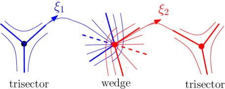
Figure 10: Cartoon of a shearless-parabolic LCS composed of nearly neutral squeezing (blue) and stretching (red) tensorline segments of the Cauchy–Green tensor field that connect wedge and trisector singularities.

Finally, we note that it can be shown [30] that the shearless-parabolic LCS are null-geodesics of a pseudo-Riemannian (Lorentzian) metric given by $g(\,\cdot\,,\,\cdot\,)(r)=\langle\,\cdot\,,D_{t_{0}}^{t}(r)\,\cdot\,\rangle\equiv 0$, which justifies calling the above a geodesic theory.

A.4 Some details on implementation

Singularities of the CG tensor points where the zero-level sets of the scalar functions $f=C_{11}-C_{22}$ and $g=C_{12}$ intersect, where $C_{ij}$ is the $(i,j)$th entry of $C$. These intersections can be found by linearly interpolating $f$ and $g$ along the edges of a numerical grid [28]. To filter out spurious intersections produced by numerical noise, Farazmand et al. [30] propose to consider only parts of the zero level set of $f$ and $g$ on which $|\lambda_{1}\lambda_{2}-1|>1$ holds. In this paper we further restrict the search of singularities to a band around the mean Eulerian axis of the Malvinas Current.

The classification of singularities may be conveniently carried out using the geometric procedure proposed by Farazmand et al. [30]. This procedure exploits the distinguishing geometric aspect of a trisector singularity with three separatrices emanating from it. Near the singularity, these separatrices are close to straight lines. As a consequence, the separatrices will be approximately perpendicular to a small circle centered at the singularity. With this in mind, a small circular neighbourhood of radius $r>0$ is selected around a singularity. With a rotating radius vector $\mathbf{r}$ of length $r$, one computes the absolute value of the cosine of the angle between $\mathbf{r}$ and $\xi_{1}$. The singularity is classified as a trisector if $\mathbf{r}$ is orthogonal to $\xi_{1}$ at exactly three points of the circle, and parallel to $\xi_{1}$ at three other points, which mark separatrices of the trisector. Singularities not passing this test for trisectors are classified as wedges.

The numerical detection of trisector–wedge connections proceeds by tracking the separatrices leaving a trisector, and monitoring whether they enter the attracting sector of a small circle surrounding a wedge.

Appendix B Probabilistic tools

B.1 Transfer operator

Assume that tracer evolution on a flow domain $X$ is governed by an advection–diffusion process. A tracer initially delta-concentrated at position $x\in X$ therefore evolves passively $\mathcal{T}$ units of time to a probability density $K(x,\cdot)\geq 0$. Normalizing so that the probability of getting somewhere from $x$ is 1, i.e., $\smash{\int_{X}K(x,y)\operatorname{d}\!{y}=1}$, $K(x,y)$ represents a stochastic kernel. A general initial density $f(x)\geq 0$, $\smash{\int_{X}f(x)\operatorname{d}\!{x}=1}$, evolves to

$$\mathscr{P}f(y)=\int_{X}K(x,y)f(x)\operatorname{d}\!{x},$$ (B.1)

where $\mathscr{P}$ is a linear transformation of the space of densities $D(X)$ to itself, a Markov operator known as the Perron–Frobenious operator or, more generally, a transfer operator [43]. Note that if $\xi_{t}$ is a random tracer position distributed a time $t$ uniformly in set $A\subset X$, i.e., $\xi_{t}\sim\smash{\frac{\mathbf{1}_{A}}{\operatorname{area}(A)}}$ where and $\mathbf{1}_{A}(x)=1$ for $x\in A$ and 0 otherwise, then the probability to be found in $B\subset X$ after $\mathcal{T}$ units of time is given by:

$$\operatorname{\mathrm{Pr}}[\xi_{t+\mathcal{T}}\in B\mid\xi_{t}\in A]=\frac{\int_{B}\mathscr{P}\frac{\mathbf{1}_{A}(y)}{\operatorname{area}(A)}\operatorname{d}\!{y}}{\int_{A}\frac{\mathbf{1}_{A}(x)}{\operatorname{area}(A)}\operatorname{d}\!{x}}=\frac{1}{\operatorname{area}(A)}\int_{A}\int_{B}K(x,y)\,\operatorname{d}\!{y}\operatorname{d}\!{x}.$$ (B.2)

Figure 11: The discrete action of the transfer operator $\mathscr{P}$ describing an advection–diffusion process in flow domain $X$ over the time interval $[t,t+\mathcal{T}]$ is represented by an $N\times N$ matrix $P$ of transitional probabilities of tracer particles of moving between boxes $\{B_{1},\dotsc,B_{N}\}$ covering $X$ from time $t$ to time $t+\mathcal{T}$.

B.2 Transition matrix

Suppose that we are presented with tracer data in the form of trajectories of individual tracer particles. One can evaluate the action of $\mathscr{P}$ on $f$ through a discretization of the Lagrangian dynamics using Ulam’s method [85]. This consists in partitioning the domain $X$ into a grid of $N$ connected boxes $\{B_{1},\dotsc,B_{N}\}$ and projecting functions in $D(X)$ onto a finite-dimensional space $V_{N}$ approximating $D(X)$ and spanned by indicator functions on the grid. Specifically, $f(x)\approx\sum_{1}^{N}f_{i}\smash{\frac{\mathbf{1}_{B_{i}}(x)}{\operatorname{area}(B_{i})}}$ where $f_{i}=\smash{\int_{B_{i}}}f(x)\operatorname{d}\!{x}$. The discrete action of $\mathscr{P}$ on $V_{N}$ is described by an $N\times N$ matrix, called a transition matrix, with components given by

$$P_{ij}=\int_{B_{j}}\mathscr{P}\frac{\mathbf{1}_{B_{i}}(y)}{\operatorname{area}(B_{i})}\operatorname{d}\!{y}=\operatorname{\mathrm{Pr}}[\xi_{t+\mathcal{T}}\in j\mid\xi_{t}\in B_{i}].$$ (B.3)

By considering a sufficiently large number of particles, the components of $P$ can be estimated as [36]

$$P_{ij}\approx\frac{\mbox{\# of particles in $B_{i}$ at any $t$ that evolve to $B_{j}$ at $t+T$}}{\mbox{\# of particles in $B_{i}$ at any $t$}}.$$ (B.4)

The matrix $P$ defines a Markov-chain representation of the dynamics, with the components $P_{ij}$ equal to one-step conditional transition probabilities of moving between boxes, which represent the states of the chain. The evolution of the discrete representation of $f(x)\in D(X)$, i.e., a vector $\mathbf{f}=(f_{1}\,\cdots\,f_{N})$ of probability since $\smash{\sum_{i=1}^{N}f_{i}=1}$, is calculated under left multiplication,

$$\mathbf{f}^{(k)}=\mathbf{f}P^{k},\quad k=1,2,\dotsc.$$ (B.5)

B.3 Irreducibility, aperiodicity, and attracting sets

Because the transition matrix $P$ is (row) stochastic, i.e., $\smash{\sum_{j=1}^{N}}P_{ij}$ for every $i$, the vector $\mathbf{1}$ of ones is a right eigenvector with eigenvalue $\lambda=1$ (i.e., $P\mathbf{1}=\mathbf{1}$), which is maximal. The associated nonunique left eigenvector $\mathbf{p}$ is invariant (because $\mathbf{p}P=\mathbf{p}$) and nonnegative (by the Perron–Frobenius theorem [45]).

If $P$ is irreducible (i.e., $\exists\,n_{ij}<\infty:\smash{(P^{n_{ij}})_{ij}>0}$, meaning that all states in the Markov chain communicate) and aperiodic (i.e., $\exists\,i:\gcd\{n\geq 0:(P^{n})_{ii}>0\}=1$, meaning that no state is revisited cyclically), then the eigenvalue $\lambda=1$ is simple, the corresponding left eigenvector $\mathbf{p}$ is strictly positive, and (scaled to a probability vector) $\smash{\mathbf{p}=\lim_{k\uparrow\infty}\mathbf{f}P^{k}}$ for any initial probability vector $\mathbf{f}$.

Suppose that $P$ is irreducible on some class of states $S\subset\{1,\dotsc,N\}$. We call $S$ an absorbing closed communicating class if $\smash{P_{ij}}=0$ for all $i\in S$, $j\notin S$, and $\smash{P_{ij}}>0$ for some $i\notin S$, $j\in S$; cf. Froyland et al. [34]. The set $B_{S}=\smash{\bigcup_{i\in S}}B_{i}\subset X$ forms an approximate time-asymptotic forward-invariant attracting set for trajectories starting in $\smash{X=\bigcup_{i=1}^{N}B_{i}}$

B.4 Communication

In practice a Markov chain can be viewed as a directed graph with vertices in the graph corresponding to states in the chain, and directed arcs in the graph corresponding to one-step transitions of positive probability. This allows one to apply Tarjan’s algorithm [70] to assess communication within a chain. Specifically, the Tarjan algorithm takes such a graph as input and produces a partition of the graph’s vertices into the graph’s strongly connected components. A directed graph is strongly connected if there is a path between all pairs of vertices. A strongly connected component of a directed graph is a maximal strongly connected subgraph and by definition also a maximal communicating class of the underlying Markov chain.

B.5 Almost-invariant sets

Revealing those regions in which trajectories tend to stay for a long time before entering another region is key to assessing connectivity in a flow. Such forward time-asymptotic almost-invariant sets and their corresponding backward-time basins of attraction can be framed [34] by inspecting eigenvectors of $P$ with $\lambda\approx 1$.

The magnitude of the eigenvalues quantifies the geometric rates at which eigenvectors decay. Those left eigenvectors with $\lambda$ closest to 1 are the slowest to decay and thus represent the most long-lived transient modes [52, 53]. For a given $\lambda\approx 1$, a forward time-asymptotic almost-invariant set will be identified with the support of similarly valued and like-sign elements in the left eigenvector. Regions where the magnitude of the left eigenvector is greatest are the most dynamically disconnected and take the longest times to transit to other almost-invariant sets.

B.6 Lagrangian geography

The multiple backward-time basins of attraction are identified by boxes where the corresponding right eigenvectors take approximately constant values (cf. Koltai [54] for the simpler single basin case). Decomposition of the ocean flow into weakly disjoint basins of attraction for time-asymptotic almost-invariant attracting sets using the above eigenvector method has been shown [34, 35, 36] to form the basis of a Lagrangian geography of the ocean, where the boundaries between basins are determined from the Lagrangian circulation itself, rather than from arbitrary geographical divisions.

The number of provinces in a geography will depend on the number of right eigenvectors considered. A large gap in the eigenspectrum of $P$ provides a cutoff criterion for eigenvector analysis, as provinces extracted from eigenvectors with eigenvalues on the right of the gap will have significantly shorter retention times than those extracted from eigenvectors on the left of the gap.

B.7 Retention time

Consider $\mathbf{p}_{A}P|_{A}=\lambda_{A}\mathbf{p}_{A}$, where $P|_{A}$ is $P$ restricted to some set $A\subset X$ and $\lambda_{A}$ is the largest eigenvalue of $P|_{A}$. If $P$ is irreducible, $\lambda_{A}<1$ and $\mathbf{p}_{A}\geq 0$. Assume that a tracer trajectory starts in $A$. If the trajectory is conditioned on being retained in $A$, it will asymptotically distribute as $\mathbf{p}_{A}$, where $\mathbf{p}_{A}$ has been normalized to a probability vector. Such a $\mathbf{p}_{A}$ is called a quasi-stationary distribution [71]. The probability of the random time $\mathfrak{T}$ to exit $A$ to be longer than $k\mathcal{T}$ is equal to the probability of the trajectory to remain in $A$ after $k$ applications of $P$, conditioned on being initially in $A$ and distributed as $\mathbf{p}_{A}$. This is thus

$$\operatorname{\mathrm{Pr}}[\mathfrak{T}>k\mathcal{T}]=\operatorname{\mathrm{Pr}}[\xi_{t+k\mathcal{T}}\in A\mid\xi_{t}\in A]=\frac{\sum_{i}(\mathbf{p}_{A}(P|_{A})^{k})_{i}}{\sum_{i}(\mathbf{p}_{A})_{i}}=\lambda_{A}^{k}.$$ (B.6)

Now note that

$$\sum_{0}^{\infty}\operatorname{\mathrm{Pr}}[\mathfrak{T}>k\mathcal{T}]=\sum_{0}^{\infty}k\operatorname{\mathrm{Pr}}[\mathfrak{T}=k\mathcal{T}].$$ (B.7)

Therefore, the expectation of the random exit time is

$$\operatorname{\mathrm{Ex}}[\mathfrak{T}]=\mathcal{T}\cdot\sum_{0}^{\infty}k\operatorname{\mathrm{Pr}}[\mathfrak{T}=k\mathcal{T}]=\mathcal{T}\cdot\sum_{0}^{\infty}\lambda_{A}^{k}=\frac{\mathcal{T}}{1-\lambda_{A}},$$ (B.8)

which provides an average measure of retention time in $A$.

Appendix C Symmetric stability

Here we adopt a coordinate system with $\mathbb{R}^{3}\{x,y,z\}$ with $z$ pointing upward. Dropping out $y$ dependencies, Cho et al. [75] show that the inviscid, unforced, nonhydrostatic, Boussinesq equations on an $f$ plane form a Lie–Poisson system on $\varphi:=(\omega_{y},m,b)$ with Hamiltonian (energy)

$$\mathscr{E}[\varphi]=-\int\big{(}\tfrac{1}{2}\psi\omega_{y}+fxm+zb\big{)}\operatorname{d}\!{x}\operatorname{d}\!{z}.$$ (C.1)

Here $\omega_{y}:=\partial_{z}u-\partial_{x}w$ is the vorticity in the $y$-direction, which in terms of the streamfuction $\psi$ reads $\omega_{y}=\nabla^{2}\psi$, where $\nabla:=(\partial_{x},\partial_{z})$; $m:=v+fx$, $b:=-g\rho/\rho_{0}$ is the buoyancy, where $g$ is gravity, and $\rho$ and $\rho_{0}$ density and reference (constant) density, respectively; and integration is on a closed domain or the whole plane with appropriate decaying conditions at infinity. Explicitly,

$$\partial_{t}\omega_{y} = [\omega_{y},\psi]+[m,fx]+[b,z],$$ (C.2)

$$\partial_{t}m = [m,\psi],$$ (C.3)

$$\partial_{t}b = [b,\psi],$$ (C.4)

using the Lie–Poisson bracket $\{\mathscr{A},\mathscr{B}\}:=\sum_{i}\int\varphi^{i}[\delta\mathscr{A}/\delta\varphi^{i},\delta\mathscr{B}/\delta\varphi^{i}]\operatorname{d}\!{x}\operatorname{d}\!{z}$ for admissible functionals $\mathscr{A},\mathscr{B}[\varphi]$ where $[\,,]$ is the Jacobian bracket.

The Casimirs of the systems are of the form

$$\mathscr{C}[\varphi]=\int C(m,b)\operatorname{d}\!{x}\operatorname{d}\!{z}$$ (C.5)

for all $C(\cdot,\cdot)$. Their conservation is a consequence of the material conservation of $m$ and $b$ by the flow. Note that the potential vorticity

$$q:=(\omega_{x},f+\omega_{z})\cdot\nabla b\equiv[m,b],$$ (C.6)

so is materially conserved.

A steady baroclinic parallel flow in thermal wind balance $f\partial_{z}V=\partial_{x}B$ represents an equilibrium of the system, including $V(x,z)=S_{0}^{2}z/f$ and $B(x,z)=S_{0}^{2}x+N_{0}^{2}z$ (where $S_{0}^{2}$ and $N_{0}^{2}>0$ are arbitrary constants) as originally considered by Hoskins [77]. Convexity of the conserved pseudoenergy

$$\mathscr{H}[\delta\varphi;\Phi]:=(\mathscr{E}+\mathscr{C})[\omega,m,b]-(\mathscr{E}+\mathscr{C})[0,M,B]$$ (C.7)

guarantees stability of the basic flow under finite-amplitude perturbations of arbitrary shape [86, 87].

Using

$$C(m,b)=\left(m+\frac{f}{\partial_{x}M\partial_{z}M}b\right)^{2}+\frac{\partial_{x}M}{Q}b^{2},$$ (C.8)

where

$$Q=[M,B]=N^{2}(f+\partial_{x}V)-f(\partial_{z}V)^{2}$$ (C.9)

is the basic flow’s potential vorticity with $N^{2}:=\partial_{z}B$ the basic flow’s Brunt–Väisälä frequency squared, Cho et al. [75] show that there exist constants $0<c_{-}\leq c_{+}<\infty$ such that

$$\|\delta\varphi\|^{2}_{t>t_{0}}\leq\mathscr{H}|_{t>t_{0}}=\mathscr{H}|_{t=t_{0}}\leq\frac{c_{+}}{c_{-}}\|\delta\varphi\|^{2}_{t=t_{0}}$$ (C.10)

where

$$\|\delta\varphi\|^{2}:=\frac{1}{2}\int\big{(}|\nabla\delta\psi|^{2}+c_{-}\delta m^{2}+c_{-}N^{-2}\delta b^{2}\big{)}\operatorname{d}\!{x}\operatorname{d}\!{z},$$ (C.11)

iff

$$\mathrm{Ri}:=\frac{N^{2}}{(\partial_{z}V)^{2}}>\frac{1}{1+\partial_{x}V/f}>0$$ (C.12)

where Ri is the Richardson number (cf. also Mu et al. [76]). Conditions (C.12) guarantee convexity of (C.7) and thus normed (i.e., Lyapunov) stability.

Cho et al. [75] use a virial functional [88] to further show that (C.12) are both sufficient and necessary conditions for stability. We note that, for a stably stratified fluid ($N^{2}>0$), (C.12) reduce to $fQ>0$, which is preserved under the flow. Thus $fQ<0$ is both necessary and sufficient for instability.

The necessary and sufficient condition for nonlinear stability $fQ>0$ clearly includes the sufficient condition for the stability of the basic state $V(x,z)=S_{0}^{2}z/f$ and $B(x,z)=S_{0}^{2}x+N_{0}^{2}z$ under $y$-independent infinitesimally small normal-mode perturbations originally derived by Hoskins [77].

References

- [1] Friocourt, Y., Drijfhout, S., Blanke, B. & Speich, S. Water mass export from Drake Passage to the Atlantic, Indian, and Pacific Oceans: A Lagrangian model analysis. J. Phys. Oceanogr. 35, 1206–1222 (2005).
- [2] Longhurst, A. Ecological Geography of the Sea (Academic Press, San Diego., San Diego, 1998).
- [3] Acha, E. M., Mianzan, H. W., Guerrero, R. A., Favero, M. & Bava, J. Marine fronts at the continental shelves of austral South America: Physical and ecological processes. J. Mar. Syst. 44, 83–105 (2004).
- [4] Matano, R. P. On the separation of the Brazil Current from the coast. Journal of Physical Oceanography 23, 79–90 (1993).
- [5] Goni, G. J., Kamholz, S., Garzoli, S. L. & Olson, D. B. Dynamics of the Brazil/Malvinas Confluence based on inverted echo sounders and altimetry. J. Geophys. Res. 101, 16273–16289 (1996).
- [6] Davis, R. E., Killworth, P. D. & Blundell, J. R. Comparison of Autonomous Lagrangian Circulation Explorer and fine resolution Antarctic model results in the South Atlantic. J. Geophys. Res. 101, 855–884 (1996).
- [7] Saraceno, M., Provost, C., Piola, A. R., Bava, J. & Gagliardini, A. Brazil Malvinas Frontal System as seen from 9 years of advanced very high resolution radiometer data. J. Geophys. Res. 109, C05027 (2004).
- [8] Piola, A. R. et al. Malvinas-slope water intrusions on the northern Patagonia continental shelf. Ocean Sci. 6, 345–359 (2010).
- [9] Piola, A. R., Franco, B. C., Palma, E. D. & Saraceno, M. Multiple jets in the Malvinas Current. J. Geophys. Res. 118, doi:10.1002/jgrc.20170. (2013).
- [10] Franco, B. C., Piola, A. R., Rivas, A. L., Baldoni, A. & Pisoni, J. P. Multiple thermal fronts near the Patagonian shelf break. Geophys. Res. Lett. 35, L02607 (2008).
- [11] Rypina, I. I. et al. On the Lagrangian dynamics of atmospheric zonal jets and the permeability of the stratospheric polar vortex. J. Atmos. Sci. 64, 3595–3610 (2007).
- [12] Beron-Vera, F. J., Olascoaga, M. J., Brown, M. G., Koçak, H. & Rypina, I. I. Invariant-tori-like Lagrangian coherent structures with application to geophysical flows. Chaos 20, 017514 (2010).
- [13] Beron-Vera, F. J. The role of jets as transport barriers in the Earth’s stratosphere. J. Phys.: Conf. Ser. 318, 072002 (2011).
- [14] Beron-Vera, F. J., Olascoaga, M. J., Brown, M. G. & Koçak, H. Zonal jets as meridional transport barriers in the subtropical and polar lower stratosphere. J. Atmos Sci. 69, 753–767 (2012).
- [15] Olascoaga, M. J. et al. Drifter motion in the Gulf of Mexico constrained by altimetric Lagrangian Coherent Structures. Geophys. Res. Lett. 40, 6171–6175 (2013).
- [16] Beron-Vera, F. J. et al. Zonal jets as transport barriers in planetary atmospheres. J. Atmos. Sci. 65, 3316–3326 (2008).
- [17] Hadjighasem, A. & Haller, G. Geodesic transport barriers in Jupiter’s atmosphere: a video-based analysis. SIAM Review 58, 69–89 (2016).
- [18] Bower, A. S., Rossby, H. T. & Lillibridge, J. L. The Gulf Stream—barrier or blender? J. Phys. Oceanogr. 15, 24–32 (1985).
- [19] Ferrari, R. & Nikurashin, M. Suppression of eddy diffusivity across jets in the Southern Ocean. Journal of Physical Oceanography 40, 1501–1519 (2010).
- [20] Marshall, J., Shuckburgh, E., Jones, H. & Hill, C. Estimates and implications of surface eddy diffusivity in the Southern Ocean derived from tracer transport. J. Phys. Oceanogr. 36, 1806–1821 (2006).
- [21] Beron-Vera, F. J. Mixing by low- and high-resolution surface geostrophic currents. J. Geophys. Res. 115, C10027 (2010).
- [22] Rypina, I. I., J.Pratt, L. & Lozier, M. S. Near-surface transport pathways in the North Atlantic Ocean: Looking for throughput from the Subtropical to the Subpolar Gyre. J. Phys. Oceanogr. 41, 911–925 (2011).
- [23] Huhn, F., von Kameke, A., Pérez-Muñuzuri, V., Olascoaga, M. J. & Beron-Vera, F. J. The impact of advective transport by the South Indian Ocean Countercurrent on the Madagascar plankton bloom. Geophys. Res. Lett. 39, L0662 (2012).
- [24] Haller, G. & Yuan, G. Lagrangian coherent structures and mixing in two-dimensional turbulence. Physica D 147, 352–370 (2000).
- [25] Haller, G. & Beron-Vera, F. J. Geodesic theory of transport barriers in two-dimensional flows. Physica D 241, 1680–1702 (2012).
- [26] Farazmand, M. & Haller, G. Attracting and repelling Lagrangian coherent structures from a single computation. Chaos 23, 023101 (2013).
- [27] Beron-Vera, F. J., Wang, Y., Olascoaga, M. J., Goni, G. J. & Haller, G. Objective detection of oceanic eddies and the Agulhas leakage. J. Phys. Oceanogr. 43, 1426–1438 (2013).
- [28] Haller, G. & Beron-Vera, F. J. Coherent Lagrangian vortices: The black holes of turbulence. J. Fluid Mech. 731, R4 (2013).
- [29] Haller, G. & Beron-Vera, F. J. Addendum to ‘Coherent Lagrangian vortices: The black holes of turbulence’. J. Fluid Mech. 755, R3 (2014).
- [30] Farazmand, M., Blazevski, D. & Haller, G. Shearless transport barriers in unsteady two-dimensional flows and maps. Physica D 278-279, 44–57 (2014).
- [31] Karrasch, D., Huhn, F. & Haller, G. Automated detection of coherent Lagrangian vortices in two-dimensional unsteady flows. Proc. Royal Soc. A 471, 20140639 (2014).
- [32] Karrasch, D. Attracting Lagrangian coherent structures on Riemannian manifolds. Chaos 25, 087411 (2015).
- [33] Haller, G. Climate, black holes and vorticity: How on Earth are they related? SIAM News 49, 1–2 (2016).
- [34] Froyland, G., Stuart, R. M. & van Sebille, E. How well-connected is the surface of the global ocean? Chaos 24, 033126 (2014).
- [35] Miron, P. et al. Lagrangian dynamical geography of the Gulf of Mexico. Scientific Reports 7, 7021 (2017).
- [36] Miron, P. et al. Lagrangian geography of the deep Gulf of Mexico. J. Phys. Oceanogr. doi:0.1175/JPO-D-18-0073.1 (2018).
- [37] Olascoaga, M. J. et al. Connectivity of Pulley Ridge with remote locations as inferred from satellite-tracked drifter trajectories. Journal of Geophysical Research 123, 5742–5750 (2018).
- [38] Dellnitz, M. & Junge, O. Almost invariant sets in Chua’s circuit. Internat. J. Bifur. Chaos 7, 2475–2485 (1997).
- [39] Dellnitz, M. & Junge, O. On the approximation of complicated dynamical behavior. SIAM J. Numer. Anal. 36, 491–515 (1999).
- [40] Froyland, G. & Dellnitz, M. Detecting and locating near-optimal almost-invariant sets and cycles. SIAM J. Sci. Comput. 24, 1839–1863 (2003).
- [41] Froyland, G. Statistically optimal almost-invariant sets. Physica D 200, 205–219 (2005).
- [42] Froyland, G. & Padberg, K. Almost-invariant sets and invariant manifolds — connecting probabilistic and geometric descriptions of coherent structures in flows. Physica D 238, 1507–1523 (2009).
- [43] Lasota, A. & Mackey, M. C. Chaos, Fractals, and Noise: Stochastic Aspects of Dynamics, vol. 97 of Applied Mathematical Sciences (Springer, New York, 1994), 2nd edn.
- [44] Kemeny, J. G. & Snell, J. L. Finite Markov Chains (Springer-Verlag, 1976).
- [45] Horn, R. A. & Johnson, C. R. Matrix Analysis (Cambridge University Press, 1990).
- [46] Norris, J. Markov Chains (Cambridge University Press, 1998).
- [47] del-Castillo-Negrete, D. & Morrison, P. J. Chaotic transport by Rossby waves in shear flow. Phys. Fluids A 5, 948–965 (1993).
- [48] Delshams, A. & de la Llave, R. KAM theory and a partial justification of Greene’s criterion for non-twist maps. SIAM J. Math. Anal. 31, 1,235–1,269 (2000).
- [49] Rypina, I. I. et al. Robust transport barriers resulting from strong Kolmogorov–Arnold–Moser stability. Phys. Rev. Lett. 98, 104102 (2007).
- [50] Simon-Miller, A. A. et al. Longitudinal variation and waves in Jupiter’s south equatorial wind jet. Icarus 218, 817–830 (2012).
- [51] Hsu, C. S. Cell-to-cell mapping. A Method of Global Analysis for Nonlinear Systems, vol. 64 of Applied Mathematical Sciences (Springer-Verlag, New York, 1987).
- [52] Froyland, G. Computer-assisted bounds for the rate of decay of correlations. Commun. Math. Phys. 189, 237–257 (1997).
- [53] Pikovsky, A. & Popovych, O. Persistent patterns in deterministic mixing flows. Europhys. Lett. 61, 625–631 (2003).
- [54] Koltai, P. A stochastic approach for computing the domain of attraction without trajectory simulation. In Dynamical Systems, Differential Equations and Applications, 8th AIMS Conference. Suppl., vol. 2, 854–863 (2011).
- [55] Rio, M.-H., Guinehut, S. & Gilles, L. New CNES–CLS09 global mean dynamic topography computed from the combination of GRACE data, altimetry, and in situ measurements. Journal of Geophysical Research 116, C07018 (2011).
- [56] Le Traon, P.-Y. et al. Use of satellite observations for operational oceanography: recent achievements and future prospects. Journal of Operational Oceanography 8, s12–s27 (2015).
- [57] Fu, L. L., Chelton, D. B., Le Traon, P.-Y. & Morrow, R. Eddy dynamics from satellite altimetry. Oceanography 23, 14–25 (2010).
- [58] Pascual, A., Faugere, Y., Larnicol, G. & Le Traon, P.-Y. Improved description of the ocean mesoscale variability by combining four satellite altimeters. Geophys. Res. Lett. 33, L02611 (2006).
- [59] Beron-Vera, F. J., Olascoaga, M. J. & Goni, G. J. Surface ocean mixing inferred from different multisatellite altimetry measurements. J. Phys. Oceanogr. 40, 2466–2480 (2010).
- [60] Samelson, R. M. Fluid exchange across a meandering jet. J. Phys. Oceanogr. 22, 431–440 (1992).
- [61] Arnold, V. I., Kozlov, V. V. & Neishtadt, A. I. Mathematical aspects of classical and celestial mechanics. In Dynamical Systems III, vol. 3 of Encyclopedia of Mathematical Sciencies, 518 (Springer-Verlag, Berlin Heidelberg, 2006), third edn.
- [62] Lumpkin, R. & Pazos, M. Measuring surface currents with Surface Velocity Program drifters: the instrument, its data and some recent results. In Griffa, A., Kirwan, A. D., Mariano, A., Özgökmen, T. & Rossby, T. (eds.) Lagrangian Analysis and Prediction of Coastal and Ocean Dynamics, chap. 2, 39–67 (Cambridge University Press, 2007).
- [63] Sybrandy, A. L. & Niiler, P. P. WOCE/TOGA Lagrangian drifter contruction manual. Tech. Rep. SIO Reference 91/6, Scripps Institution of Oceanography, La Jolla, California (1991).
- [64] Lumpkin, R. et al. Removing spurious low-frequency variability in drifter velocities. J. Atm. Oce. Tech. 30, 353–360 (2012).
- [65] Beron-Vera, F. J., Olascoaga, M. J. & Lumpkin, R. Inertia-induced accumulation of flotsam in the subtropical gyres. Geophys. Res. Lett. 43, 12228–12233 (2016).
- [66] LaCasce, J. H. Statistics from Lagrangian observations. Progr. Oceanogr. 77, 1–29 (2008).
- [67] Maximenko, A. N., Hafner, J. & Niiler, P. Pathways of marine debris derived from trajectories of Lagrangian drifters. Mar. Pollut. Bull. 65, 51–62 (2012).
- [68] van Sebille, E., England, E. H. & Froyland, G. Origin, dynamics and evolution of ocean garbage patches from observed surface drifters. Environ. Res. Lett. 7, 044040 (2012).
- [69] McAdam, R. & van Sebille, E. Surface connectivity and interocean exchanges from drifter-based transition matrices. Journal of Geophysical Research: Oceans 123, 514–532 (2018).
- [70] Tarjan, R. Depth-first search and linear graph algorithms. SIAM J. Comput. 1, 146–160 (1972).
- [71] Brémaud, P. Markov chains, vol. 31 of Gibbs Fields Monte Carlo Simulation Queues, Texts in Applied Mathematics (Springer, New York, 1999).
- [72] Dellnitz, M., Froyland, G., Horenkam, C., Padberg-Gehle, K. & Sen Gupta, A. Seasonal variability of the subpolar gyres in the southern ocean: a numerical investigation based on transfer operators. Nonlinear Process. Geophys. 16, 655–663 (2009).
- [73] Saraceno, M., Provost, C. & Piola, A. R. On the relationship of satellite retrieved surface temperature fronts and chlorophyll-a in the Western South Atlantic. J. Geophys. Res. 110, C11016 (2005).
- [74] Saraceno, M., Provost, C. & Lebbah, M. Biophysical Regions identification using an artificial neuronal network: a case study in the South Western Atlantic. Advances in Space Research 37, 793–805 (2006).
- [75] Cho, H. R., Shepherd, T. G. & Vladimirov, V. A. Application of the direct Liapunov method to the problem of symmetric stability in the atmosphere. Journal of the Atmospheric Sciences 50, 822–836 (1993).
- [76] Mu, M., Shepherd, T. G. & Swanson, K. On nonlinear symmetric stability and the nonlinear saturation of symmetric instability. J. Atmos. Sci. 53, 2918–2923 (1996).
- [77] Hoskins, B. J. The role of potential vorticty in symmetric stability and instability. Quart. J. R. Met. Soc. 100, 480–482 (1974).
- [78] Saunders, P. M. & King, B. A. Bottom currents derived from a shipborne ADCP on WOCE cruise A11 in the South Atlantic. J. Phys. Oceanogr. 25, 329–347 (1995).
- [79] Aref, H. Stirring by chaotic advection. J. Fluid Mech. 143, 1–21 (1984).
- [80] Magalhães, J. M. & da Silva, J. C. B. Internal waves along the Malvinas Current: Evidence of transcritical generation in satellite imagery. Oceanography 30, 110–119 (2017).
- [81] Thomas, L. N. et al. Symmetric instability, inertial oscillations, and turbulence at the gulf stream front. Journal of Physical Oceanography 46, 197–217 (2016).
- [82] Delmarcelle, T. & Hesselink, L. Topology of symmetric, second-order tensor fields. In Proceedings of the Conference on Visualization ’94, VIS ’94, 140–147 (IEEE Computer Society Press, 1994).
- [83] Kratz, A., Auer, C., Stommel, M. & Hotz, I. Visualization and analysis of second-order tensors: Moving beyond the symmetric positive-definite case. Computer Graphics Forum 32, 49–74 (2013).
- [84] Spivak, M. A Comprehensive Introduction to Differential Geometry, vol. 3 (Publish or Perish, Inc., 1999), 3rd edn.
- [85] Ulam, S. M. A Collection of Mathematical Problems. Interscience tracts in pure and applied mathematics (Interscience, 1960).
- [86] Arnold, V. I. Conditions for nonlinear stability of stationary plane curvilinear flows of an ideal fluid. Dokl. Akad. Nauk. SSSR 162, 975–978 (1965). Engl. transl. Sov. Math. 6: 773-777 (1965).
- [87] Holm, D. D., Marsden, J. E., Ratiu, T. & Weinstein, A. Nonlinear stability of fluid and plasma equilibria. Phys. Rep. 123, 1–116 (1985).
- [88] Chandrasekhar, S. Ellipsoidal figures of equilibrium (Yale University Press, 1969).