Floquet approach to $\mathbb{Z}_{2}$ lattice gauge theories with ultracold atoms in optical lattices

Quantum simulation has the potential to investigate gauge theories in strongly-interacting regimes, which are up to now inaccessible through conventional numerical techniques. Here, we take a first step in this direction by implementing a Floquet-based method for studying $\mathbb{Z}_{2}$ lattice gauge theories using two-component ultracold atoms in a double-well potential. For resonant periodic driving at the on-site interaction strength and an appropriate choice of the modulation parameters, the effective Floquet Hamiltonian exhibits $\mathbb{Z}_{2}$ symmetry. We study the dynamics of the system for different initial states and critically contrast the observed evolution with a theoretical analysis of the full time-dependent Hamiltonian of the periodically-driven lattice model. We reveal challenges that arise due to symmetry-breaking terms and outline potential pathways to overcome these limitations. Our results provide important insights for future studies of lattice gauge theories based on Floquet techniques.

Lattice gauge theories (LGTs) Wilson (1974); Kogut (1979) are fundamental for our understanding of quantum many-body physics across different disciplines ranging from condensed matter Wen (2004); Levin and Wen (2005); Lee et al. (2006); Ichinose and Matsui (2014) to high-energy physics Aoki et al. (2017). However, theoretical studies of LGTs can be extremely challenging in particular in strongly-interacting regimes, where conventional computational methods are limited Troyer and Wiese (2005); Alford et al. (2008). To overcome these limitations alternative numerical tools are currently developed, which enable out-of-equilibrium and finite density computations Buyens et al. (2016); Bañuls et al. (2017); Silvi et al. (2017); Gazit et al. (2017). In parallel, the rapid progress in the field of quantum simulation Weimer et al. (2010); Blatt and Roos (2012); Gross and Bloch (2017); Romero et al. (2017) has sparked a growing interest in designing experimental platforms to explore the rich physics of LGTs Tagliacozzo et al. (2013); Wiese (2013); Zohar et al. (2015); Dalmonte and Montangero (2016); Notarnicola et al. (2015); Kasper et al. (2017); Kuno et al. (2017); Zhang et al. (2018). State-of-the-art experiments are now able to explore the physics of static Aidelsburger et al. (2018) as well as density-dependent gauge fields Clark et al. (2018) and have engineered controlled few-body interactions Anderlini et al. (2007); Trotzky et al. (2008); Dai et al. (2017), which are the basis for many proposed schemes to realize LGTs. First studies of the Schwinger model have been performed with quantum-classical algorithms Klco et al. (2018) and a digital quantum computer composed of four trapped ions Martinez et al. (2016). The challenge for analog quantum simulators mainly lies in the complexity to engineer gauge-invariant interactions between matter and gauge fields.

Here, we explore the dynamics of a minimal model for $\mathbb{Z}_{2}$ LGTs coupled to matter with ultracold atoms in periodically-driven double-well potentials Barbiero et al. (2019). An alternative technique was recently proposed for digital quantum simulation Zohar et al. (2017). $\mathbb{Z}_{2}$ LGTs are of high interest in condensed matter physics Horn et al. (1979); Ju and Balents (2013); Gazit et al. (2017); González-Cuadra et al. (2019) and topological quantum computation Kitaev (2003). Our scheme is based on density-dependent laser-assisted tunneling techniques Keilmann et al. (2011); Greschner and Santos (2015); Bermudez and Porras (2015); Sträter et al. (2016). We use a mixture of bosonic atoms in two different internal states to encode the matter and gauge field degrees of freedom. The interaction between these states is engineered via resonant periodic modulation Goldman et al. (2015); Goldman and Dalibard (2014); Bukov et al. (2015); Eckardt (2017) of the on-site potential at the inter-species Hubbard interaction Ma et al. (2011); Chen et al. (2011); Meinert et al. (2016); Görg et al. (2019). By choosing suitable modulation parameters, the effective Floquet model exhibits a $\mathbb{Z}_{2}$ symmetry Barbiero et al. (2019). We present a detailed study of this effective Floquet model defined on a double well, which constitutes the basic building block of the LGT. We discuss the relation between the observed dynamics and the ideal model and reveal the potential impact of symmetry-breaking terms.

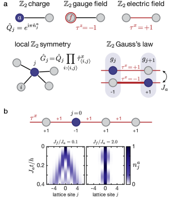
Figure 1: 1D $\mathbb{Z}_{2}$ lattice gauge theory coupled to matter. Circles indicate lattice sites, which are empty (gray) or occupied by a matter particle (blue). Red circles and the thickness of red links illustrate the expectation value of the link operators, $\tau^{z}$ and $\tau^{x}$. a Elementary ingredients: $\mathbb{Z}_{2}$ charge $\hat{Q}_{j}\!=\!\text{e}^{i\pi\hat{n}_{j}^{a}}$, $\mathbb{Z}_{2}$ gauge field $\hat{\tau}^{z}_{\langle j,j+1\rangle}$, $\mathbb{Z}_{2}$ electric field $\hat{\tau}^{x}_{\langle j,j+1\rangle}$, and local symmetry operator $\hat{G}_{j}$ with conserved quantities $g_{j}$. Here $i\!:\!\langle i,j\rangle$ denotes all lattice sites $i$ connected to site $j$ via a nearest-neighbor link, denoted as $\langle i,j\rangle$. Matter and gauge fields are implemented using two different species, denoted as $a$ (blue) and $f$ (red). Matter-gauge coupling occurs with strength $J_{a}$. b Dynamics of the 1D model (1) for different values of $J_{f}/J_{a}$ calculated with exact diagonalization of a system with 13 sites based on Eq. (1). The initial state is a single matter particle located on site $j\!=\!0$ and the gauge field is in an eigenstate of the electric field.

In order to understand the observed phenomena, it is instructive to consider the properties of an extended one-dimensional (1D) $\mathbb{Z}_{2}$ LGT, as captured by the Hamiltonian

$$\hat{H}_{\mathbb{Z}_{2}}\!=\! -\sum\limits_{j}J_{a}\left(\hat{\tau}_{\langle j,j+1\rangle}^{z}\hat{a}_{j}^{\dagger}\hat{a}_{j+1}^{\phantom{\dagger}}+\text{h.c.}\right)$$

$$-\sum\limits_{j}J_{f}\hat{\tau}_{\langle j,j+1\rangle}^{x}.$$ (1)

Here $\hat{a}_{j}^{\dagger}$ describes the creation of a matter particle on lattice site $j$ and the Pauli operators ${\bf\hat{\tau}}_{\langle j,j+1\rangle}$, defined on the links between neighboring lattice sites, encode the gauge field degrees of freedom. The elementary ingredients of this $\mathbb{Z}_{2}$ LGT are illustrated in Fig. 1a. Note that the illustrations of the $\mathbb{Z}_{2}$ gauge field and $\mathbb{Z}_{2}$ electric field are related to the physical implementation of the building block, which is discussed later in the text. The matter field has a charge $\hat{Q}_{j}\!=\!\text{e}^{i\pi\hat{n}_{j}^{a}}$ on site $j$, which is given by the parity of the site occupation, with $\hat{n}_{j}^{a}\!=\!\hat{a}_{j}^{\dagger}\hat{a}_{j}^{\phantom{\dagger}}$ the number operator. The dynamics of the matter field is coupled to the $\mathbb{Z}_{2}$ gauge field $\hat{\tau}^{z}_{\langle j,j+1\rangle}$ with an amplitude $J_{a}$. The energy scale associated with the electric field $\hat{\tau}^{x}_{\langle j,j+1\rangle}$ is $J_{f}$.

The model Hamiltonian (1) commutes with the lattice gauge transformations defined by the local symmetry operators

$$\hat{G}_{j}\!=\!\hat{Q}_{j}\prod_{i:\langle i,j\rangle}\hat{\tau}_{\langle i,j\rangle}^{x},\qquad\left[\hat{H},\hat{G}_{j}\right]\!=\!0\ \ \forall j,$$ (2)

where $\prod_{i:\langle i,j\rangle}$ denotes the product over all nearest-neighbor links connected to lattice site $j$. The eigenvalues of $\hat{G}_{j}$ are $g_{j}\!=\!\pm 1$. The dynamics of the model is constrained by $\mathbb{Z}_{2}$ Gauss’s law, $\hat{G}_{j}|\psi\rangle\!=\!g_{j}|\psi\rangle$, in analogy to electrodynamics. Since the local values $g_{j}$ are conserved, the motion of $\mathbb{Z}_{2}$ charges is coupled to a change of the $\mathbb{Z}_{2}$ electric field lines on the link connecting the two lattice sites. Gauss’s law effectively separates the Hilbert space into different subsectors, which are characterized by a set of conserved quantities $\{g_{j}\}$. The two configurations sketched in Fig. 1a (lower right) belong to the same subsector and illustrate the basic matter-gauge coupling according to Gauss’s law. Lattice sites with $g_{j}\!=\!-1$ are interpreted as local static background charges (Supplementary Information). Different subsectors can be explored by preparing suitable initial states.

In order to gain more insight into the physics of the 1D model (1), we consider a system initially prepared in an eigenstate of the electric field operator, with $\tau^{x}\!=\!+1$ on all links, and a single matter particle located on site $j=0$. For this initial state $g_{j}\!=\!+1$, $\forall j\neq 0$ and $g_{j}\!=\!-1$ for $j\!=\!0$ (Fig. 1b). In the limit of vanishing electric field energy $J_{f}\rightarrow 0$, the matter particle can tunnel freely along the 1D chain, thereby changing the electric field on all traversed links. For $J_{f}\neq 0$, tunneling of the matter particle is detuned due to the energy of the electric field and the matter particle is bound to the location of the static background charge at $j=0$. In this regime the energy of the system scales linearly with the distance between the static charge and the matter particle, which we interpret as a signature of confinement (Supplementary Information).

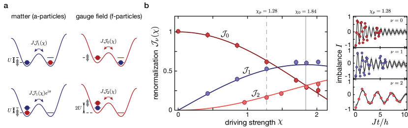
Figure 2: Driving scheme for $\mathbb{Z}_{2}$ LGTs on a double well. a Effective tunneling processes for the matter field (blue, $a$) and gauge field (red, $f$) particle. For $\phi=0$, hopping of $a$-particles occurs for resonant one-photon processes at $\hbar\omega\!\approx\!U$ with an effective amplitude $J\mathcal{J}_{1}(\chi)$, where $U$ is the inter-species on-site interaction. Depending on the position of the $f$-particle, the $a$-particle acquires a phase shift of $\pi$, which realizes the matter-gauge coupling. Tunneling of the $f$-particle is renormalized by zero- or induced via two-photon processes, with amplitudes $J\mathcal{J}_{0}(\chi)$ and $J\mathcal{J}_{2}(\chi)$ depending on the $a$-particle’s position. b Experimental results for the renormalization of the tunnel couplings $\mathcal{J}_{\nu}(\chi)$ for single-particle $\nu$-photon processes $\nu\!=\!\{0,1,2\}$, with $\omega\!=\!2\pi\times 4122\,$Hz and $J/h\!\approx\!0.5\,$kHz. The solid lines are the Bessel functions, where $\chi$ was calibrated by fitting the zeroth-order Bessel function to the dark red data points (Supplementary Information). The time traces of the imbalance $I$ are fitted with sinusoidal functions taking into account an inhomogeneous tilt distribution (solid black line) and shown for exemplary traces at $\chi_{p}\!=\!1.28$ (dashed vertical line, left panel) on the right. The error bars and the gray shading are the $1\sigma$-confidence interval obtained from a bootstrap analysis of 1000 repetitions (Supplementary Information). The solid gray vertical line marks the value $\chi_{0}$, where $\mathcal{J}_{0}(\chi_{0})\!=\!\mathcal{J}_{2}(\chi_{0})$.

Here, we engineer the elementary interactions of the $\mathbb{Z}_{2}$ model on a two-site lattice following Ref. Barbiero et al. (2019). The matter and gauge fields are implemented using two different species denoted as $a$- and $f$-particles, which are realized by two Zeeman levels of the hyperfine ground-state manifold of ⁸⁷Rb, $\left|a\right>\equiv\left|F\!=\!1,m_{F}\!=\!-1\right>$ and $\left|f\right>\equiv\left|F\!=\!1,m_{F}\!=\!+1\right>$. We prepare one $a$- and one $f$-particle in each two-site system. The matter field is associated with the $a$-particle. The $\mathbb{Z}_{2}$ gauge field is the number imbalance $\hat{\tau}^{z}_{\langle j,j+1\rangle}\!=\!\hat{n}^{f}_{j+1}-\hat{n}^{f}_{j}$ of the $f$-particle and the $\mathbb{Z}_{2}$ electric field corresponds to tunneling of the $f$-particle, $\hat{\tau}^{x}_{\langle j,j+1\rangle}\!=\!\hat{f}_{j}^{\dagger}\hat{f}_{j+1}^{\phantom{\dagger}}+\hat{f}_{j+1}^{\dagger}\hat{f}_{j}^{\phantom{\dagger}}$, where $\hat{f}_{j}^{\dagger}$ is the creation operator of an $f$-particle on site $j$ and $\hat{n}^{f}_{j}\!=\!\hat{f}_{j}^{\dagger}\hat{f}_{j}^{\phantom{\dagger}}$ is the corresponding number-occupation operator. An extension of our scheme to realize extended 1D LTGs is presented in the Supplementary Information. It requires exactly one $f$-particle per link, while the density of $a$-particles (fermions or hard-core bosons) can take arbitrary values.

The driving scheme is based on a species-dependent double-well potential with tunnel coupling $J$ between neighboring sites and an energy offset $\Delta_{f}$ only seen by the $f$-particle. Experimentally, it is realized with a magnetic-field gradient, making use of the opposite magnetic moments of the two states $|a\rangle$ and $|f\rangle$ (Supplementary Information). In the limit of strong on-site interactions $U\gg J$, first-order tunneling processes are suppressed but can be restored resonantly with a periodic modulation at the resonance frequency $\hbar\omega=\sqrt{U^{2}+4J^{2}}\approx U$. The full time-dependent Hamiltonian can be expressed as

$$\hat{H}(t)\!= -J\left(\hat{a}^{\dagger}_{2}\hat{a}^{\phantom{\dagger}}_{1}+\hat{f}^{\dagger}_{2}\hat{f}^{\phantom{\dagger}}_{1}+\textrm{h.c.}\right)$$ (3)

$$+U\sum\limits_{j\!=\!1,2}\hat{n}^{a}_{j}\hat{n}^{f}_{j}+\Delta_{f}\hat{n}_{1}^{f}$$

$$+A\cos{\left(\omega t+\phi\right)}\,(\hat{n}^{a}_{1}+\hat{n}^{f}_{1}),$$

where $A$ is the modulation amplitude and $\phi$ is the modulation phase. For resonant modulation $\hbar\omega\approx U$ and in the high-frequency limit $\hbar\omega\gg J$, the lowest order of the effective Floquet Hamiltonian contains renormalized tunneling matrix elements for both $a$- and $f$-particles Goldman and Dalibard (2014); Bukov et al. (2015); Eckardt (2017). For general modulation parameters, the amplitudes and phases are operator-valued and explicitly depend on the site-occupations. For certain values of the modulation phase ($\phi\!=\!0$ or $\pi$), however, these expressions simplify and realize the $\mathbb{Z}_{2}$ model. The driving scheme can be understood by considering the individual photon-assisted tunneling processes of $a$- and $f$-particles in situations, where one of the two particles is localized on a particular site of the double well. This generates an occupation-dependent energy offset for the other particle, which is equal to the on-site Hubbard interaction $U$ (Fig. 2a). For all configurations tunneling is resonantly restored for energy differences $\nu\hbar\omega$ between neighboring sites with renormalized tunneling $J\mathcal{J}_{\nu}(\chi)\text{e}^{i\nu\phi}$; here $\nu$ is an integer, $\mathcal{J}_{\nu}$ is the $\nu$th-order Bessel function of the first kind and $\chi\!=\!A/(\hbar\omega)$ the dimensionless driving parameter.

For $\phi=0$, we find that the strength of $a$-particle tunneling is density-independent $J_{a}=J|\mathcal{J}_{\pm 1}(\chi)|$, however, depending on the position of the $f$-particle, the on-site energy difference between neighboring sites is either $+U$ or $-U$ (Fig. 2a). This results in a sign-dependence of the renormalized tunneling $\pm J_{a}$, which stems from the property of odd Bessel functions $\mathcal{J}_{-\nu}(\chi)\!=\!(-1)^{\nu}\mathcal{J}_{\nu}(\chi)$ (Supplementary Information) and is central to our implementation of the $\mathbb{Z}_{2}$ symmetry Barbiero et al. (2019). It allows us to write the renormalized hopping of $a$-particles as $J_{a}\,\hat{\tau}^{z}_{\langle 1,2\rangle}$. Note that we drop the link-index from now on to simplify notations, ${\bf\hat{\tau}}\equiv{\bf\hat{\tau}}_{\langle 1,2\rangle}$.

Tunneling of $f$-particles becomes real-valued, with an amplitude that only weakly depends on the position of the $a$-particle. Due to the species-dependent tilt $\Delta_{f}=U$ the on-site energy difference between neighboring sites is either $\Delta_{f}\!-\!U\!=\!0$ or $\Delta_{f}\!+\!U\!=\!2U$ (Fig. 2a). Therefore, tunneling is renormalized via zero- and two-photon processes, resulting in the real-valued tunneling matrix elements $J\mathcal{J}_{0}(\chi)$ and $J\mathcal{J}_{2}(\chi)$. To lowest order, the effective double-well Hamiltonian takes the form

$$\hat{H}_{\text{eff}}\!=\!-J_{a}\,\hat{\tau}^{z}\left(\hat{a}^{\dagger}_{2}\hat{a}^{\phantom{\dagger}}_{1}+\hat{a}^{\dagger}_{1}\hat{a}^{\phantom{\dagger}}_{2}\right)-\hat{J}_{f}\,\hat{\tau}^{x},$$ (4)

where $\hat{J}_{f}$ depends on the position of the $a$-particle

$$\hat{J}_{f}\!=\!J\mathcal{J}_{0}(\chi)\,\hat{n}^{a}_{1}+J\mathcal{J}_{2}(\chi)\,\hat{n}^{a}_{2}.$$ (5)

The density dependence of $\hat{J}_{f}$ can be avoided by choosing the dimensionless driving strength $\chi$ such that $\mathcal{J}_{0}(\chi_{0})\!=\!\mathcal{J}_{2}(\chi_{0})$, which occurs, e.g. at $\chi_{0}\!\approx\!1.84$. Then, Eq. (4) reduces to the two-site version of the $\mathbb{Z}_{2}$ LGT described by Hamiltonian (1). Note that the double-well model defined in Eq. (4) is $\mathbb{Z}_{2}$-symmetric for all values of the driving strength $\chi$.

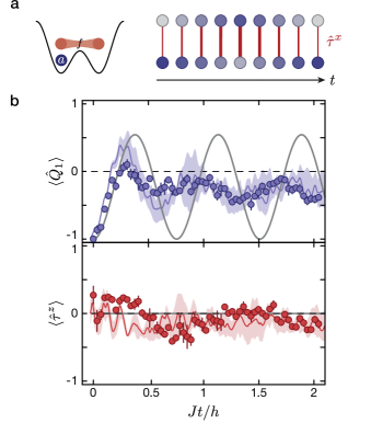
Figure 3: Dynamics of the matter-gauge system prepared initially in an eigenstate of the electric field $\hat{\tau}^{x}$. a Illustration of the gauge invariant initial state $\left|\psi_{0}^{x}\right>\!=\!|a,0\rangle\otimes\left(|f,0\rangle+|0,f\rangle\right)/\sqrt{2}$ and the expected dynamics according to Hamiltonian (4). b Measured expectation values of the $\mathbb{Z}_{2}$ charge $\langle\hat{Q}_{1}\rangle$ (blue points) and $\mathbb{Z}_{2}$ gauge field $\langle\hat{\tau}^{z}\rangle$ (red points) for $\omega\!=\!2\pi\!\times\!4320\,$Hz. Each data point represents the mean of at least three individual experimental results and the error bars denote the standard deviation. The blue and red lines and shadings show a numerical analysis using time-dependent exact-diagonalization, which includes averaging of the observables in the presence of an inhomogeneous tilt distribution $\Delta(x,y,z)$ approximated by a normal distribution with standard deviation $\Delta_{\sigma}/h\!=\!0.44(2)\,$kHz, which was independently calibrated (Supplementary Information). The blue and red solid line is the median and the shading represents the $1\sigma$-confidence interval obtained with a bootstrap analysis of 1000 repetitions. All calculations are performed using the independently calibrated experimental parameters, $J/h\!=\!587(3)\,$Hz, $\Delta_{f}/h\!=\!4.19(3)\,$kHz, $U/h\!=\!3.85(7)\,$kHz and taking into account additional terms that appear in the extended Bose-Hubbard model (Supplementary Information). The gray solid lines are the ideal dynamics according to Eq. (4) and Eq. (6).

The experimental setup consists of a 3D optical lattice generated at wavelength $\lambda_{s}\!=\!767\,$nm. Along the $x$-axis an additional standing wave with wavelength $2\lambda_{s}\!=\!1534\,$nm is superimposed to create a superlattice potential. For deep transverse lattices and suitable superlattice parameters, an array of isolated double-well potentials is realized, where all dynamics is restricted to the two double-well sites (Supplementary Information). The periodic drive is generated by modulating the amplitude of an additional lattice with wavelength $2\lambda_{s}$, whose potential maxima are aligned relative to the double-well potential in order to modulate only one of the two sites. This enables the control of the modulation phase, which is set to $\phi\!=\!0$ or $\pi$.

We first study the renormalization of the tunneling matrix elements for the relevant $\nu$-photon processes Keay et al. (1995); Lignier et al. (2007); Sias et al. (2008); Mukherjee et al. (2015); Meinert et al. (2016) with a single atom on each double well (Fig. 2b). For every measurement, the atom is initially localized on the lower-energy site with a potential energy difference $\Delta_{\nu}\!\approx\!\nu\hbar\omega$ to the higher-energy site, where $\nu\in\{0,1,2\}$. Then, the resonant modulation is switched on rapidly at frequency $\omega$ and we evaluate the imbalance $I\!=\!n_{2}-n_{1}$ as a function of the evolution time, where $n_{j}$ is the density on site $j$. These densities were determined using site-resolved detection methods Trotzky et al. (2008). Note, this technique provides an average of this observable over the entire 3D array of double-well potentials. Hence, an overall harmonic confinement and imperfect alignment of the lattice laser beams introduces an inhomogeneous tilt distribution $\Delta(x,y,z)$, which leads to dephasing of the averaged dynamics. The renormalized tunneling amplitude is obtained from the oscillation frequency of the imbalance and by numerically taking into account the tilt distribution $\Delta(x,y,z)$ [Fig. 2b]. We find that our data agrees well with the expected Bessel-type behavior for the $\nu$-photon processes (Supplementary Information). Moreover, these measurements enable us to directly determine the value of the modulation amplitude, for which $\mathcal{J}_{0}(\chi_{0})\!=\!\mathcal{J}_{2}(\chi_{0})$, as indicated by the vertical line in Fig. 2b.

In order to study the dynamics of the $\mathbb{Z}_{2}$ double-well model (4), we prepare two different kinds of initial states, where the gauge field particle is either prepared in an eigenstate of the electric field $\hat{\tau}^{x}$ (Fig. 3) or the gauge field operator $\hat{\tau}^{z}$ (Fig. 4a). In both cases the matter particle is initially localized on site $j\!=\!1$.

First, we consider the state $\left|\psi_{0}^{x}\right>\!=\!|a,0\rangle\otimes\left(|f,0\rangle+|0,f\rangle\right)/\sqrt{2}$ (Fig. 3a), where the gauge field particle is in a symmetric superposition between the two sites. This state is an eigenstate of $\hat{G}_{j}$ defined in Eq. (2). The corresponding eigenvalues are $g_{1}\!=\!-1$ and $g_{2}\!=\!+1$. After initiating the dynamics by suddenly turning on the resonant modulation, we expect that the matter particle starts to tunnel to the neighboring site ($j\!=\!2$) according to the matter-gauge coupling. Depending on the energy of the electric field $J_{f}$, this process can be energetically detuned and the matter particle does not fully tunnel to the other site. Solving the dynamics according to Hamiltonian (4) analytically, gives:

$$\langle\hat{Q}_{1}(t)\rangle \!=\!-\frac{J_{f}^{2}+J_{a}^{2}\cos\left(2t\sqrt{J_{f}^{2}+J_{a}^{2}}\right)}{J_{f}^{2}+J_{a}^{2}}.$$ (6)

The maximum value of $\langle\hat{Q}_{1}\rangle$ is limited to $(J_{a}^{2}-J_{f}^{2})/(J_{a}^{2}+J_{f}^{2})$. The experimental configuration is well suited to explore the regime $J_{f}/J_{a}=\mathcal{J}_{0}(\chi_{0})/\mathcal{J}_{1}(\chi_{0})\!\approx\!0.54$, which corresponds to an intermediate regime between the two limiting cases discussed in Fig. 1c. These cases can also be understood at the level of the two-site model. In the weak electric field regime ($J_{f}/J_{a}\ll 1$) the matter particle tunnels freely between the two sites, while in the limit of a strong electric field ($J_{f}/J_{a}\gg 1$) the matter particle remains localized.

In the experiment we can directly access the value of the charge operator $\hat{Q}_{j}\!=\!\text{e}^{i\pi\hat{n}_{j}^{a}}$ and the link operator $\hat{\tau}^{z}\!=\!\hat{n}^{f}_{2}-\hat{n}^{f}_{1}$ via site- and state-resolved detection techniques Trotzky et al. (2008). They provide direct access to the state-resolved density on each site of the double well $n_{j}^{a}$ and $n_{j}^{f}$, averaged over the entire 3D array of double-well realizations. The experimental results are shown in Fig. 3b for $U/J\!=\!6.6$ and $\phi\!=\!0$. As expected, we find that the charge oscillates, while the dynamics of the $f$-particle is strongly suppressed. We observe a larger characteristic oscillation frequency for the $a$-particle compared to the prediction of Eq. (6) [gray line, Fig. 3b]. This is predominantly caused by an inhomogeneous tilt distribution $\Delta(x,y,z)$ present in our system. Taking the inhomogeneity into account, the numerical analysis of the full time-dependence according to Eq. (3) [solid blue line, Fig. 3b] shows good agreement with the experimental results. The fast oscillations both in the data and the numerics are due to the micromotion at non-stroboscopic times.

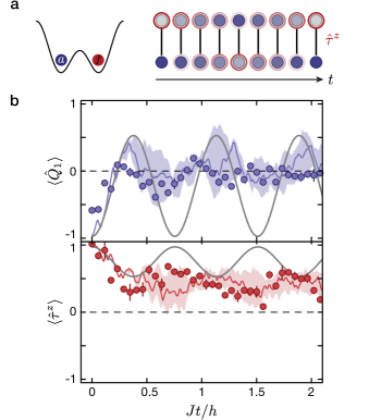
Figure 4: Dynamics of the matter-gauge system prepared initially in an eigenstate of the gauge field $\hat{\tau}^{z}$. a Schematic of the initial state $\left|\psi_{0}^{z}\right>\!=\!|a,0\rangle\otimes|0,f\rangle$ and the expected dynamics. Brightness of the red circles illustrate the expectation value of $\hat{\tau}^{z}$. b Measured expectation values of the $\mathbb{Z}_{2}$ charge $\langle\hat{Q}_{1}\rangle$ (blue points) and the $\mathbb{Z}_{2}$ gauge field $\langle\hat{\tau}^{z}\rangle$ (red points) for $\omega\!=\!2\pi\!\times\!4314\,$Hz. Each data point represents the mean of at least three individual experimental results and the error bars denote the standard deviation. The blue and red lines and shadings show a numerical analysis using time-dependent exact-diagonalization, with $J/h\!=\!578(3)\,$Hz, $\Delta_{f}/h\!=\!4.19(3)\,$kHz, $U/h\!=\!3.85(7)\,$kHz and $\Delta_{\sigma}/h\!=\!0.46(2)\,$kHz as explained in the caption of Fig. (3b) and the Supplementary Information. The blue and red solid line is the median and the shading represents the $1\sigma$-confidence interval obtained with a bootstrap analysis of 1000 repetitions. The gray solid lines are the ideal dynamics according to Eq. (4) and Eq. (6).

The $f$-particle is initially prepared in an eigenstate of the electric field operator $\hat{\tau}^{x}$, which corresponds to an equal superposition of the particle on both sites of the double-well potential, i.e. $\langle\hat{\tau}^{z}(t\!=\!0)\rangle\!=\!0$. The $\mathbb{Z}_{2}$ electric field follows the oscillation of the matter particle in a correlated manner to conserve the local quantities $g_{j}$. At the same time the expectation value of the gauge field $\langle\hat{\tau}^{z}(t)\rangle$ is expected to remain zero at all times. This is a non-trivial result, which is a direct consequence of the $\mathbb{Z}_{2}$-symmetry constraints. In contrast, a resonantly driven double-well system with $\Delta_{f}\!=\!0$, which does not exhibit $\mathbb{Z}_{2}$ symmetry, would show dynamics with equal oscillation amplitudes for the $a$- and $f$-particle. In the experiment we clearly observe suppressed dynamics for the $f$-particle, which is a signature of the experimental realization of the $\mathbb{Z}_{2}$ symmetry (Fig. 3b). Deviations between the time-dependent numerical analysis and the experimental results are most likely due to an imperfect initial state, residual energy offsets, and finite ramp times.

In a second set of experiments we study the dynamics where the gauge field particle is initialized in an eigenstate of the gauge field operator $\hat{\tau}^{z}$, while the matter particle is again localized on site $j\!=\!1$, $\left|\psi_{0}^{z}\right>\!=\!|a,0\rangle\otimes|0,f\rangle$ (Fig. 4a). Here, the system is in a coherent superposition of the two subsectors with $g_{1}=-g_{2}\!=\!\pm 1$ and the expectation value of the locally conserved operators are $\langle\hat{G}_{1}\rangle\!=\!\langle\hat{G}_{2}\rangle\!=\!0$. Note that there is no coupling between different subsectors according to Hamiltonian (4). The basic dynamics can be understood in the two limiting cases of the model. For $J_{f}\ll J_{a}$ the electric field vanishes and the system is dominated by the gauge field $\hat{\tau}^{z}$. In this limit, a system prepared in an eigenstate of $\hat{\tau}^{z}$ will remain in this eigenstate because $\hat{\tau}^{z}$ commutes with Hamiltonian (4) for $J_{f}\!=\!0$. In the opposite regime ($J_{f}\!\gg\!J_{a}$), where the electric field dominates, $\langle\hat{\tau}^{z}\rangle$ oscillates between the two eigenvalues. The dynamics of the $\mathbb{Z}_{2}$ charge on the other hand is still determined by Eq. (6). In the experiment we probe the intermediate regime at $J_{f}/J_{a}\!\approx\!0.54$ for $U/J\!=\!6.7$ and $\phi\!=\!\pi$ (Fig. 4b). The dynamics agrees with the ideal evolution (gray line, Fig. 4b) for short times. For longer times it deviates due to the averaging over the inhomogeneous tilt distribution $\Delta(x,y,z)$, which is well captured by the full time-dynamics according to Hamiltonian (3) [red and blue lines, Fig. 4b]. Notably, $\langle\hat{\tau}^{z}\rangle$ exhibits a non-zero average value.

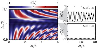
Figure 5: Finite-frequency corrections to the effective Floquet Hamiltonian (4). Stroboscopic dynamics of the expectation value of the local $\mathbb{Z}_{2}$-symmetry operator $\langle\hat{G}_{1}\rangle$ for $|\psi^{x}_{0}\rangle$, with $g_{1}=-1$, based on Hamiltonian (3) for different driving frequencies $\omega$. The panels on the right show examples of the time traces for $\hbar\omega\!\approx\!1.04\,U$ and $\hbar\omega\!=\!1.01\,U$.

An important requirement for quantum simulations of gauge theories is the exact implementation of the local symmetry constraints in order to assure that $\langle\hat{G}_{j}\rangle$ is conserved for all times. Since we do not have direct access to $\langle\hat{G}_{j}\rangle$ experimentally, we study the implications of symmetry-breaking terms numerically. The dominant contribution stems from the inhomogeneous tilt distribution $\Delta(x,y,z)$, which, however, can be avoided in future experiments by generating homogeneous box potentials. The second type of gauge-variant terms are coupling processes that do not fulfill the constraints of Gauss’s law. These are correlated two-particle tunneling and nearest-neighbor interactions, which are known to exist in interacting lattice models Scarola and Das Sarma (2005). For our experimental parameters these terms are on the order of $0.03\,J$ and can be neglected for the timescale of the observed dynamics (Supplementary Information). The same gauge-variant processes appear in the higher-order terms of the Floquet expansion for finite $U/J$  Goldman and Dalibard (2014); Bukov et al. (2015); Eckardt (2017). We study them analytically by calculating the first-order terms of the expansion and comparing them to numerics (Supplementary Information). In Fig. 5 we show the numerically-calculated dynamics for the initial state $|\psi^{x}_{0}\rangle$ (Fig. 3a) according to the full time-dependent Hamiltonian [Eq. (3)] for $U/J\!=\!7$, similar to the experimental values (Fig. 5). We find that in this regime the driving frequency is crucial and defines the timescale for which the $\mathbb{Z}_{2}$ symmetry of the model remains. In particular there is an optimal value around $\hbar\omega\!\approx\!1.01\,U$, where the value of $\langle\hat{G}_{1}\rangle$ deviates by $<10\%$ even for long evolution times.

In summary, we have studied the dynamics of a minimal model for $\mathbb{Z}_{2}$ LGTs. Our observations are well described by a full time-dependent analysis of the 3D system. Moreover, we find non-trivial dynamics of the matter and gauge field in agreement with predictions from the ideal $\mathbb{Z}_{2}$ LGT. We further reached a good understanding of relevant symmetry-breaking terms. The dominant processes we identified are species-independent energy offsets between neighboring sites and correlated two-particle tunneling terms Scarola and Das Sarma (2005), which can be suppressed in future experiments. We have further provided important insights into the applicability of Floquet schemes. While the Floquet parameters can be fine-tuned in certain cases to ensure gauge invariance, this complication can be avoided by reaching the high-frequency limit Goldman and Dalibard (2014); Bukov et al. (2015); Eckardt (2017) to minimize finite-frequency corrections. In experiments this could be achieved using Feshbach resonances to increase the inter-species scattering length. This, however, comes at the cost of enhanced correlated tunneling processes, which in turn can be suppressed by increasing the lattice depth (Supplementary Information). Numerical studies further indicate that certain experimental observables are robust to gauge-variant imperfections Banerjee et al. (2013); Kühn et al. (2014), which may facilitate future experimental implementations. We anticipate that the double-well model demonstrated in this work serves as a stepping stone for experimental studies of $\mathbb{Z}_{2}$ LGTs coupled to matter in extended 1D and 2D systems, which can be realized by coupling many double-well links along a 1D chain (Supplementary Information) or in a ladder configuration Barbiero et al. (2019). Finally, the use of state-dependent optical lattices could further enable an independent tunability of the matter- and gauge-particle tunneling terms.

V.1 Acknowledgements

We acknowledge insightful discussions with M. Dalmonte, A. Trombettoni and M. Lohse. This work was supported by the Deutsche Forschungsgemeinschaft (DFG, German Research Foundation) under project number 277974659 via Research Unit FOR 2414 and under project number 282603579 via DIP, the European Commission (UQUAM Grant No. 5319278) and the Nanosystems Initiative Munich (NIM, Grant No. EXC4). The work was further funded by the Deutsche Forschungsgemeinschaft (DFG, German Research Foundation) under Germany’s Excellence Strategy – EXC-2111 – 390814868. Work in Brussels was supported by the FRS-FNRS (Belgium) and the ERC Starting Grant TopoCold. F. G. additionally acknowledges support by the Gordon and Betty Moore foundation under the EPIQS program and from the Technical University of Munich – Institute for Advanced Study, funded by the German Excellence Initiative and the European Union FP7 under grant agreement 291763, from the DFG grant No. KN 1254/1-1, and DFG TRR80 (Project F8). F. G. and E. D. acknowledge funding from Harvard-MIT CUA, AFOSR-MURI Quantum Phases of Matter (grant FA9550-14-1-0035), AFOSR-MURI: Photonic Quantum Matter (award FA95501610323) and DARPA DRINQS program (award D18AC00014).

V.2 Author contributions

C.S., F.G., N.G. and M.A. planned the experiment and performed theoretical calculations. C.S. and M.B. performed the experiment and analyzed the data with M.A. All authors discussed the results and contributed to the writing of the paper.

V.3 Data availability

The data that support the plots within this paper and other findings of this study are available from the corresponding author upon reasonable request.

V.4 Code availability

The code that supports the plots within this paper are available from the corresponding author upon reasonable request.

S.XI Interpretation: static local background charges

Below Eq. (2) in the main text we introduced the notion of “static local background charges” for lattice sites, where $g_{j}=-1$. Here, we want to briefly explain this in a more formal manner. In this interpretation, we consider a second, immobile species $b$ of matter particles (corresponding to another particle flavor), which are localized on the sites with $g_{j}=-1$. If a single $b$ particle is localized on site $j$, it contributes to the $\mathbb{Z}_{2}$ charge $\hat{\tilde{Q}}_{j}=\exp[\mathrm{i}\pi(\hat{n}^{a}_{j}+\hat{n}^{b}_{j})]$, where $\hat{n}^{b}_{j}$ is the number operator for $b$ particles.

In particular, for the dynamics presented in Fig. 1b, this interpretation results in the following scenario: We initialize a single $a$-particle on the central site $j=0$ and the field in an eigenstate of the electric field, $\tau^{x}=1$, on all links. This results in $g_{j}=1$ on all sites except at $j=0$, where $g_{0}=-1$. Consequently, there is a static background charge localized at $j=0$. The $\mathbb{Z}_{2}$ Gauss’s law with the charge operator $\hat{\tilde{Q}}_{j}$ given above, then results in $\tilde{g}_{j}=1$ for all $j$, which is conventionally the physical subsector. Moreover, when the $a$-particle moves, it is connected by a string of $\mathbb{Z}_{2}$ electric-field lines to the localized $b$ particle. The energy cost of this electric field string leads to a linear string tension, which can be interpreted as a simple instant of confinement.

S.XII Effective Hamiltonian

S.XII.1 Floquet expansion

The $\mathbb{Z}_{2}$ double-well model realized in this work consists of a two-site potential with one $a$- and one $f$-particle implementing the matter and gauge field, respectively. Such a two-site two-particle model can be represented using the four basis states: $\left|1\right>\!=\!\left|a,0\right>\otimes\left|f,0\right>$, $\left|2\right>\!=\!\left|a,0\right>\otimes\left|0,f\right>$, $\left|3\right>\!=\!\left|0,a\right>\otimes\left|f,0\right>$ and $\left|4\right>\!=\!\left|0,a\right>\otimes\left|0,f\right>$, where the labels $a$ and $f$ before or after the comma mark the particle occupation on the left and right site. As described in the main text, a species-dependent energy offset $\Delta_{f}\!=\!U$ between the two sites and a species-independent resonant driving $A\cos(\omega t+\phi)$ of the on-site potential are applied, which leads to the time-dependent Hamiltonian (3) in the main text. In the new basis defined above, this Hamiltonian reads

$$\hat{H}(t)= -J\left(\left|3\right>\left<1\right|+\left|4\right>\left<2\right|+\left|4\right>\left<3\right|+\left|2\right>\left<1\right|+\mathrm{h.c.}\right)$$

$$+U\left(2\left|1\right>\left<1\right|+\left|3\right>\left<3\right|+\left|4\right>\left<4\right|\right)$$ (S.1)

$$+A\cos(\omega t+\phi)\left(2\left|1\right>\left<1\right|+\left|2\right>\left<2\right|+\left|3\right>\left<3\right|\right),$$

where the tunneling rate of both $a$- and $f$-particles is $J$ and the intra-species interaction energy is $U$.

The stroboscopic dynamics of such a time-dependent system can be described by an effective Floquet Hamiltonian represented by a series of time-independent terms in powers of $1/\omega$. The series can be truncated to lowest order in the high-frequency limit $\omega\rightarrow\infty$. Following the method presented in Goldman et al. (2015); Goldman and Dalibard (2014), we calculate the Floquet Hamiltonian $\hat{H}_{\mathrm{F}}$ up to first order. To this end, Eq. (S.1) is transformed by a unitary transformation $\left|\psi\right>\rightarrow\left|\psi^{\prime}\right>\!=\!\hat{R}(t)\left|\psi\right>$, such that the new Hamiltonian $\hat{\mathcal{H}}(t)$ does not contain divergent terms in the high-frequency limit:

$$\hat{\mathcal{H}}(t)=\hat{R}\hat{H}(t)\hat{R}^{\dagger}-\mathrm{i}\hat{R}\partial_{t}\hat{R}^{\dagger}=\sum\limits_{k\in\mathbb{Z}}\hat{\mathcal{H}}^{(k)}\mathrm{e}^{\mathrm{i}k\omega t}.$$ (S.2)

We express this transformed Hamiltonian in a Fourier-series with time-independent components $\hat{\mathcal{H}}^{(k)}$. For our model (S.1), we choose the transformation

$$\hat{R}(t)= \exp\Bigl{\{}+\mathrm{i}\omega t\left(2\left|1\right>\left<1\right|+\left|3\right>\left<3\right|+\left|4\right>\left<4\right|\right)$$ (S.3)

$$+\frac{\mathrm{i}A}{\hbar\omega}\sin(\omega t+\phi)\left(2\left|1\right>\left<1\right|+\left|2\right>\left<2\right|+\left|3\right>\left<3\right|\right)\Bigr{\}}$$

and obtain the following Fourier components

$$\hat{\mathcal{H}}^{(k)}= -J\,\Bigl{\{}\mathcal{J}_{-k-1}(\chi)\left|3\right>\left<1\right|\mathrm{e}^{\mathrm{i}(k+1)\phi}+\mathcal{J}_{k-1}(\chi)\left|1\right>\left<3\right|\mathrm{e}^{\mathrm{i}(k-1)\phi}+\mathcal{J}_{-k+1}(\chi)\left|4\right>\left<2\right|\mathrm{e}^{\mathrm{i}(k-1)\phi}+\mathcal{J}_{k+1}(\chi)\left|2\right>\left<4\right|\mathrm{e}^{\mathrm{i}(k+1)\phi}$$

$$+\mathcal{J}_{-k}(\chi)\left|4\right>\left<3\right|\mathrm{e}^{\mathrm{i}k\phi}+\mathcal{J}_{k}(\chi)\left|3\right>\left<4\right|\mathrm{e}^{\mathrm{i}k\phi}+\mathcal{J}_{-k-2}(\chi)\left|2\right>\left<1\right|\mathrm{e}^{\mathrm{i}(k+2)\phi}+\mathcal{J}_{+k-2}(\chi)\left|1\right>\left<2\right|\mathrm{e}^{\mathrm{i}(k-2)\phi}\Bigr{\}}$$ (S.4)

$$+(U-\hbar\omega)\delta_{k0}\,\Bigl{\{}2\left|1\right>\left<1\right|+\left|3\right>\left<3\right|+\left|4\right>\left<4\right|\Bigr{\}}.$$

Here $\mathcal{J}_{\nu}(\chi)$ is the $\nu$-th Bessel function of the first kind with the dimensionless driving strength $\chi\!=\!A/\hbar\omega$ and $\delta_{ij}$ the Kronecker delta. Note that in the finite-frequency regime the resonant driving frequency for a double well tilted by the energy difference $U$ is equal to the energy gap, $\hbar\omega\!=\!\sqrt{U^{2}+4J^{2}}\neq U$. In the high-frequency limit $U\gg J$, however, $\hbar\omega\simeq U$. The lowest orders of the Floquet Hamiltonian can be calculated using the components $\hat{\mathcal{H}}^{(k)}$ [Eq. (S.4)] according to

$$\hat{H}_{\mathrm{F}}=\hat{\mathcal{H}}^{(0)}+\frac{1}{\hbar\omega}\sum\limits_{k>0}\frac{1}{k}\left[\hat{\mathcal{H}}^{(+k)},\hat{\mathcal{H}}^{(-k)}\right]+\mathcal{O}\left(\frac{1}{\omega^{2}}\right).$$ (S.5)

S.XII.2 Floquet model in the infinite-frequency limit

In the limit $U/J\rightarrow\infty$, the resonant driving frequency is $\hbar\omega\!\simeq\!U$ and the diagonal terms in Eq. (S.4) vanish. The Floquet Hamiltonian (S.5) reduces to the lowest order

$$\hat{H}_{\mathrm{F}}^{0}= -J\big{\{}\mathcal{J}_{1}(\chi)\left|3\right>\left<1\right|\mathrm{e}^{\mathrm{i}(\pi+\phi)}+\mathcal{J}_{1}(\chi)\left|4\right>\left<2\right|\mathrm{e}^{-\mathrm{i}\phi}$$ (S.6)

$$+\mathcal{J}_{0}(\chi)\left|4\right>\left<3\right|+\mathcal{J}_{2}(\chi)\left|2\right>\left<1\right|\mathrm{e}^{2\phi}+\mathrm{h.c.}\bigr{\}},$$

referred to as zeroth-order Floquet Hamiltonian in the following. As discussed in the main text, different tunnel processes have different renormalizations with an additional phase factor depending on the modulation phase $\phi$. The tunnel processes $\left|3\right>\left<1\right|$ and $\left|4\right>\left<2\right|$ correspond to $a$-particle tunneling and $\left|4\right>\left<3\right|$ and $\left|2\right>\left<1\right|$ to $f$-particle tunneling. The $a$-particle’s tunneling rate is renormalized with the first-order Bessel function of the first kind $\mathcal{J}_{1}(\chi)$, while on the other hand the $f$-particle’s tunneling rate is renormalized depending on the $a$-particle’s position. The latter asymmetry can be resolved by choosing the driving strength such that $\mathcal{J}_{0}(\chi_{0})\!=\!\mathcal{J}_{2}(\chi_{0})$. This happens the first time at $\chi_{0}\approx 1.84$ (Fig. 2 in main text). When choosing the modulation phase $\phi\!=\!\{0,\pi\}$, the Floquet Hamiltonian (S.6) directly realizes the $\mathbb{Z}_{2}$ double well, where the $a$-particle’s tunnel phase is either $0$ or $\pi$ depending on the $f$-particle’s position, while tunneling of the $f$-particle is real-valued. This density-dependent phase shift reflects the sign of the effective energy offset $\pm U$ between neighboring sites experienced by the $a$-particle because of the reflection properties of the Bessel function $\mathcal{J}_{-1}(\chi)\!=\!\mathrm{e}^{\mathrm{i}\pi}\mathcal{J}_{1}(\chi)$.

S.XII.3 Floquet model including the first-order correction for finite-frequency drive

In experiments, it is generally challenging to work deep in the high-frequency limit, especially without the availability of Feshbach resonances; here, we work at $U/J\approx 6.6$. Consequently, higher order corrections become relevant. In order to study their impact on the dynamics we calculate the first-order terms of the Floquet expansion and include them in our calculations (Fig. S1). We restrict the derivation to stroboscopic time points $n\,T$ with $T\!=\!2\pi/\omega$, $n\in\mathbb{N}$ and set the driving phase to $\phi\!=\!0$.

The first-order term of the Floquet expansion can be calculated following Eq. (S.5). Note, the resonant driving frequency is now $\hbar\omega\!=\!\sqrt{U^{2}+4J^{2}}\neq U$ and the diagonal terms in $\hat{\mathcal{H}}^{0}$ become nonzero.

$$\hat{H}_{\mathrm{F}}= \begin{aligned} \hat{\mathcal{H}}^{(0)}+\frac{J^{2}}{\hbar\omega}\sum\limits_{k>0}\frac{1}{k}&\Bigl{\{}\left|3\right>\left<2\right|\bigl{(}\mathcal{J}_{-k-1}(\chi)\,\mathcal{J}_{-k-2}(\chi)+\mathcal{J}_{k}(\chi)\,\mathcal{J}_{k+1}(\chi)-\mathcal{J}_{k-1}(\chi)\,\mathcal{J}_{k-2}(\chi)-\mathcal{J}_{-k}(\chi)\,\mathcal{J}_{-k+1}(\chi)\bigr{)}+\mathrm{h.c.}\\ +&\left|4\right>\left<1\right|\bigl{(}\mathcal{J}_{-k+1}(\chi)\,\mathcal{J}_{k-2}(\chi)+\mathcal{J}_{-k}(\chi)\,\mathcal{J}_{k-1}(\chi)-\mathcal{J}_{k+1}(\chi)\,\mathcal{J}_{-k-2}(\chi)-\mathcal{J}_{+k}(\chi)\,\mathcal{J}_{-k-1}(\chi)\bigr{)}+\mathrm{h.c.}\Bigr{\}}\\ +\frac{J^{2}}{\hbar\omega}\sum\limits_{k>0}\frac{1}{k}&\Bigl{\{}\bigl{(}\left|1\right>\left<1\right|-\left|2\right>\left<2\right|\bigr{)}\bigl{(}\mathcal{J}_{k-1}(\chi)^{2}+\mathcal{J}_{k-2}(\chi)^{2}-\mathcal{J}_{-k-1}(\chi)^{2}-\mathcal{J}_{-k-2}(\chi)^{2}\bigr{)}\\ +&\bigl{(}\left|4\right>\left<4\right|-\left|3\right>\left<3\right|\bigr{)}\bigl{(}\mathcal{J}_{-k+1}(\chi)^{2}+\mathcal{J}_{-k}(\chi)^{2}-\mathcal{J}_{k+1}(\chi)^{2}-\mathcal{J}_{k}(\chi)^{2}\bigr{)}\Bigr{\}}\end{aligned}$$

$$= \hat{\mathcal{H}}^{(0)}+\hat{H}^{(1)}_{\mathrm{pair-hopping}}+\hat{H}^{(1)}_{\mathrm{detuning}}$$ (S.7)

The first-order correction contains two types of terms: a pair-tunneling term $\hat{H}^{(1)}_{\mathrm{pair-hopping}}$, which corresponds to tunneling of both particles, and a detuning term $\hat{H}^{(1)}_{\mathrm{detuning}}$, describing the deviation from the exact resonance condition.

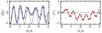
Figure S1: Finite-frequency corrections to the zeroth-order Floquet Hamiltonian. Solid lines are the time evolution of the charge $\langle\hat{Q}_{1}\rangle$ (blue) and gauge field $\langle\hat{\tau}^{z}\rangle$ (red) according to (S.8) with the two lowest-order terms of the effective Floquet Hamiltonian (S.7). Diamonds show the stroboscopic dynamics of the full time-dependent Hamiltonian (3) from the main text for resonant driving at $\hbar\omega\!=\!\sqrt{U^{2}+4J^{2}}\!\approx\!1.04\,U$ and $U/J\!=\!7$. Gray lines show the ideal solution Eq. (6) of the zeroth-order effective Hamiltonian (S.6) for $\phi=0$.

When calculating the time evolution including higher order terms, the time evolution operator $\hat{U}$ gets modified in general by both the transformation $\hat{R}$ and the kick operator $\hat{K}$ Goldman et al. (2015). However, for stroboscopic times the time-evolution operator reduces to

$$\hat{U}(0\rightarrow nT)=e^{-\mathrm{i}\hat{K}}e^{-\mathrm{i}\hat{H}_{\mathrm{F}}nT/\hbar}e^{\mathrm{i}\hat{K}}$$ (S.8)

and only depends on the stroboscopic kick operator

$$\hat{K}=\frac{1}{\mathrm{i}\hbar\omega}\sum\limits_{k>0}\frac{1}{k}\left(\hat{\mathcal{H}}^{(+k)}-\hat{\mathcal{H}}^{(-k)}\right)+\mathcal{O}\left(\frac{1}{\omega^{2}}\right).$$ (S.9)

In Fig. S1 the dynamics of the effective Floquet model including first-order corrections is compared to a full time-dependent analysis of Hamiltonian (3) from the main text. We find that for the experimental timescales and parameters, i.e. $U/J=7$, the effective model up to first order is sufficient to describe the dynamics of the system.

S.XIII Description of the experiment

S.XIII.1 Lattice setup

In the experiment, ultracold ⁸⁷Rb atoms in a three-dimensional (3D) optical lattice potential are used. The lattice consists of three mutually orthogonal standing waves with wavelength $\lambda_{\mathrm{s}}\!=\!767\,$nm and an additional lattice with $\lambda_{\mathrm{l}}\!=\!2\lambda_{\mathrm{s}}$ along the $x$-direction, which generates the superlattice potential

$$V_{\mathrm{SL}}(x)\!=\!V_{x,\mathrm{s}}\cos^{2}(k_{\mathrm{s}}x)+V_{x,\mathrm{l}}\cos^{2}(k_{\mathrm{l}}x+\varphi_{\mathrm{SL}}),$$ (S.10)

where $V_{x,\mu}$ denotes the lattice depth and $k_{\mu}\!=\!2\pi/\lambda_{\mu}$ is the wave number, with $\mu\in\{\mathrm{s},\mathrm{l}\}$. In addition, a standing wave with wavelength $\lambda_{\mathrm{l}}$ is superimposed, where the relative phase between the potentials is chosen such that the potential maxima affect only one of the double-well sites (Fig. S2). The overall potential is then given by

$$V(x)\!=\!V_{\mathrm{SL}}(x)+V_{\mathrm{mod}}\,\cos^{2}(k_{l}x-\pi/4),$$ (S.11)

with $V_{\mathrm{mod}}$ the lattice depth of the additional modulation lattice. A time-dependent modulation $V_{\mathrm{mod}}\!=\!V_{\mathrm{mod}}^{(0)}+A_{\mathrm{mod}}\cos(\omega t+\phi)$ around a mean value $V_{\mathrm{mod}}^{(0)}$ in combination with a suitable static superlattice phase $\varphi_{\mathrm{SL}}$ then generates the time-dependent Hamiltonian (S.1).

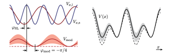
Figure S2: Lattice setup. A superlattice (black) is composed of a lattice with wavelength $\lambda_{\mathrm{s}}$ (blue) and a lattice with wavelength $\lambda_{\mathrm{l}}\!=\!2\lambda_{\mathrm{s}}$ (red) with a relative phase of $\varphi_{\mathrm{SL}}$. In addition, a second lattice with wavelength $\lambda_{\mathrm{l}}$ is superimposed with a relative phase of $\varphi_{\mathrm{mod}}\!=\!-\pi/4$, such that the on-site energy of the left double-well site can be modified by a change in the lattice depth $V_{\mathrm{mod}}$ [Eq. (S.11)] illustrated by the red and gray shadings. The dashed lines show the superlattice for $V_{\mathrm{mod}}=0$.

S.XIII.2 Measurement of the renormalization of the tunnel coupling in a driven double well

We experimentally determine the renormalization of the tunnel coupling of a single particle in a driven double well. The time-dependent Hamiltonian can be written in the basis, where the particle occupies the left $\left|L\right>$ or the right $\left|R\right>$ site of the double well:

$$\hat{H}_{\mathrm{1P}}(t)= -J^{\prime}\left(\left|L\right>\left<R\right|+\left|R\right>\left<L\right|\right)$$

$$+\left\{\Delta+A\cos(\omega t+\phi)\right\}\left|L\right>\left<L\right|,$$ (S.12)

where $J^{\prime}$ is the single-particle tunneling rate, $\Delta$ the energy offset between neighboring sites, $A$ the modulation amplitude, $\omega$ the modulation frequency and $\phi$ the modulation phase. In the high-frequency limit with resonant multi-frequency driving $\Delta\!=\!\nu\,\hbar\omega$, with $\nu\in\mathbb{Z}$, we find the Fourier components of the Floquet expansion analogous to Eq. (S.4)

$$\hat{\mathcal{H}}^{(k)}_{\mathrm{1P}}=-J^{\prime}\Bigl{\{} \mathcal{J}_{-k-\nu}(\chi)\,\mathrm{e}^{\mathrm{i}(k+\nu)\phi}\left|R\right>\left<L\right|+$$

$$\mathcal{J}_{+k-\nu}(\chi)\,\mathrm{e}^{\mathrm{i}(k-\nu)\phi}\left|L\right>\left<R\right|\Bigr{\}}.$$ (S.13)

In the infinite frequency limit $\omega\rightarrow\infty$, we can extract the renormalization of the tunnel coupling $\widetilde{J}_{\nu}\!=\!J^{\prime}|\mathcal{J}_{\nu}(\chi)|$, which scales with the $\nu$th-order Bessel function of the first kind.

We load atoms in the $\left|F\!=\!1,m_{F}\!=\!-1\right>$ state into a 3D optical lattice by performing an exponential-shaped ramp during a time segment of $50\,$ms; the final lattice depths $V_{x,\mathrm{l}}\!=\!30(1)\,E_{r,\mathrm{l}}$, $V_{y}\!=\!35(1)\,E_{r,\mathrm{s}}$ are reached within the $1/e$-time $\tau\!=\!5\,$ms, while the vertical lattice $V_{z}\!=\!50(1)\,E_{r,\mathrm{s}}$ is ramped up within $\tau_{z}\!=\!1.5\,$ms. The lattice depth is given in units of their respective recoil energy $E_{r,\mu}\!=\!\hbar^{2}k_{\mu}^{2}/2m$ with $m$ the mass of a rubidium atom and $\mu\!=\!\{\mathrm{s},\mathrm{l}\}$. Then, we use a filtering sequence to remove doubly-occupied sites by light assisted-collisions between atoms in the $|F\!=\!2,m_{F}\!=\!-1\rangle$ state. The subsequent part of the sequence is in principle not needed for this measurement but it is part of the final experimental sequence and it is kept in order to reach a comparable experimental situation. In this part the long-period lattice site is split within $15\,$ms by increasing $V_{x,\mathrm{s}}\!=\!30(1)\,E_{r,\mathrm{s}}$ together with the transversal lattices $V_{y,\mathrm{s}}\!=\!V_{z,\mathrm{s}}=60(2)\,E_{r,\mathrm{s}}$ and merged again in $15\,$ms by ramping down $V_{x,\mathrm{s}}\!=\!0$. Then, the modulation lattice is turned on at the mean value $V_{\mathrm{mod}}^{(0)}\!=\!15.0(2)\,E_{r,\mathrm{l}}$ in $20\,$ms and the superlattice phase $\varphi_{\mathrm{SL}}$ is tuned to a value such that $\Delta\gg J$. The particle localizes to one site during the subsequent splitting process, where the short lattice is ramped to $V_{x,\mathrm{s}}\!=\!40(1)\,E_{r,\mathrm{s}}$ in $10\,$ms. Subsequently, $\varphi_{\mathrm{SL}}$ is non-adiabatically changed to reach the final energy offset between the two sites $\Delta_{\nu}$ in $10\,$ms. The time evolution begins with a rapid coupling of the two sites by decreasing $V_{x,\mathrm{s}}\!=\!9.5(1)\,E_{r,\mathrm{s}}$ in $100\,\mu$s and starting the modulation with frequency $\omega\!=\!2\pi\times 4122\,$Hz. This procedure was repeated for various modulation amplitudes $A_{\mathrm{mod}}$. For the detection, we freeze the motion in $100\,\mu$s and use site-resolved band mapping to determine the site occupations $N_{\mathrm{L}}$ and $N_{\mathrm{R}}$ from which we determine the site imbalance $I\!=\!(N_{\mathrm{L}}-N_{\mathrm{R}})/(N_{\mathrm{L}}+N_{\mathrm{R}})$ Sebby-Strabley et al. (2006); Fölling et al. (2007).

For finite driving frequencies, corrections to the resonant driving condition have to be taken into account $\nu\hbar\omega\!=\!\sqrt{\Delta_{\nu}^{2}+4J^{2}}$ with $\nu\neq 0$. Thus, we have experimentally determined $\Delta_{\nu}$ using a spectroscopic measurement by varying the energy offset at constant driving frequency $\omega$. Measurements of a time-trace for different modulation amplitudes $A_{\mathrm{mod}}$ were performed for $\nu\in\{0,1,2\}$. Each resulting imbalance time-trace represents an average over the time-traces of all double wells in a 3D array. For technical reasons, each double well in this 3D array experiences different energy offsets between neighboring sites. To model this effect, we assume that these energy offsets are distributed according to

$$\mathcal{G}_{\Delta}(\delta)=\frac{1}{\sqrt{2\pi\Delta_{\sigma}^{2}}}\,\exp\left(-\frac{\delta^{2}}{2\Delta_{\sigma}^{2}}\right),$$ (S.14)

with a standard deviation $\Delta_{\sigma}$. Taking this effect into account, the renormalized tunneling rates $\widetilde{J}_{\nu}$ were extracted by fitting an average of $S\!=\!10$ sinusoidal functions

$$I_{\nu}(t)=\frac{A}{S}\sum\limits_{n\!=\!1}^{S}\sin\left(\sqrt{\delta_{n}^{2}+4\widetilde{J}_{\nu}^{2}}\,t/\hbar+\xi\right)+I_{0}$$ (S.15)

to the data, where $A$ is the oscillation amplitude, $\delta_{n}$ a random sample of the tilt distribution (S.14), $\widetilde{J}_{\nu}\!=\!J^{\prime}_{\nu}\mathcal{J}_{\nu}(\chi)$ is the renormalized tunnel coupling, $\xi$ is an initial phase due to the finite initialization ramp time, and $I_{0}$ the imbalance offset of the oscillation. The fit uses five free fit parameters: $\widetilde{J}_{\nu}$, $A$, $\Delta_{\sigma}$, $\xi$, and $I_{0}$. To estimate the confidence interval we performed a bootstrap analysis with $1000$ realizations for different sets of $\{\delta_{n}\}$, a Gaussian error in the detection of the imbalance of $0.05$ and randomly-guessed fit start values for $\widetilde{J}_{\nu}$. In Fig. 2 (main text), $\widetilde{J}_{\nu}$ is normalized to its respective bare tunnel coupling strength $J^{\prime}_{\nu}$ calculated from the double-well Wannier functions based on the calibrated lattice parameters: $J^{\prime}_{0}/h\!=\!490\,$Hz, $J^{\prime}_{1}/h\!=\!520\,$Hz and $J^{\prime}_{2}/h\!=\!563\,$Hz. They are slightly different for the three data sets, $\nu\!=\!\{0,1,2\}$. The data points and error bars in Fig. 2 show the median and the $1\sigma$-confidence interval from the bootstrap analysis. The conversion $\alpha$ of the driving amplitude $A\!=\!\alpha\,A_{\mathrm{mod}}$ is calibrated by a fit of the function $\mathcal{J}_{0}(\alpha_{\mathrm{fit}}\,A_{\mathrm{mod}}/\omega)$ to the experimental results for $\nu\!=\!0$. A comparison of the fitted to the calculated value results in $\alpha_{\mathrm{fit}}/\alpha_{\mathrm{calc}}\approx 1.09(2)$. The order of magnitude of this value is consistent for all measurements and is most likely attributed to the non-linear behavior of $\Delta(V_{\mathrm{mod}})$. In addition, also the tunneling rate depends on the value of the modulation lattice depth $J^{\prime}_{\nu}(V_{\mathrm{mod}})$ and changes therefore sightly during a driving period. These effects are especially important for large values $V_{\mathrm{mod}}\sim V_{x,\mathrm{l}}$, because the modulation lattice changes not only the on-site energy, but also the combined lattice potential’s shape $V(x)$.

S.XIII.3 Species-dependent energy offset
for the $\mathbb{Z}_{2}$ two-site model

The species-dependent energy offset is realized by a combination of a magnetic gradient and a superlattice with a relative phase $\varphi_{\mathrm{SL}}$. The magnetic gradient induces opposite energy offsets $\Delta_{\mathrm{M}}$ for the two hyperfine-states that encode the $a$- and $f$-particles, i.e. $\left|F\!=\!1,m_{F}\!=\!\mp 1\right\rangle$, because these states have opposite magnetic moments. The experimental implementation requires an energy offset of zero between neighboring sites for the $a$-particles. Thus, the species-independent energy offset from the superlattice potential is chosen, such that it compensates the tilt $\Delta_{\mathrm{M}}\!=\!-\Delta_{\mathrm{SL}}$. The energy offset between neighboring sites for the $f$-particles is then $\Delta_{f}\!=\!\Delta_{\mathrm{M}}+\Delta_{\mathrm{SL}}$, which needs to be matched with the interaction energy $U$.

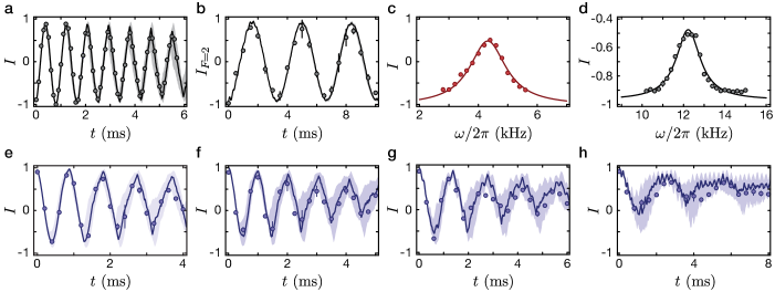
Figure S3: Parameter calibrations. a Tunnel oscillations in a symmetric double well for $V_{x,\mathrm{s}}\!=\!9.50(1)\,E_{r,\mathrm{s}}$, $V_{x,\mathrm{l}}\!=\!35(1)\,E_{r,\mathrm{l}}$, and $V_{\mathrm{mod}}\!=\!0$. The resulting single-particle tunneling rate is $J^{\prime}/h\!=\!574(3)\,$Hz. b Superexchange oscillations. c The spectroscopic measurement of the tilt $\Delta_{f}\!=\!\Delta_{\mathrm{M}}+\Delta_{\mathrm{SL}}$ leads to the resonance $\omega\!=\!2\pi\times 4.32(2)\,$kHz. d A spectroscopic measurement of the tilt induced only by the modulation lattice $V^{(0)}_{\mathrm{mod}}\!=\!15.0(1)\,E_{r,\mathrm{l}}$ leads to a resonance $\omega_{\mathrm{mod}}\!=\!2\pi\times 12.23(2)\,$kHz. e Tunnel oscillations in a symmetric configuration for the final lattice parameters $V_{x,\mathrm{s}}\!=\!9.50(1)\,E_{r,\mathrm{s}}$, $V_{x,\mathrm{l}}\!=\!35(1)\,E_{r,\mathrm{l}}$, and $V_{\mathrm{mod}}^{(0)}\!=\!15.0(2)\,E_{r,\mathrm{l}}$ in the presence of the magnetic gradient. The particle experiences a potential equivalent to the one seen by the $a$-particle. The resulting tunneling rate is $J^{\prime}/h\!=\!523(3)\,$Hz. f-h Driven tunnel oscillations in the same configuration as e for $\chi\approx 0.61$ in f, $\chi\approx 1.23$ in g, $\chi\approx 1.84$ in h.

S.XIII.4 Tight-binding description of the two-site two-particle model

The working principle of the experimental implementation for the $\mathbb{Z}_{2}$ two-site model is discussed in detail in the main text. Here, we present a tight-binding description including the full set of experimental parameters and terms from the extended Bose-Hubbard model, which are known to exist for interacting particles in lattices Scarola and Das Sarma (2005). The extended Bose-Hubbard model takes into account that the Wannier functions $w_{\mathrm{\mu}}(r)$ of particles on different sites $\mu$ overlap. Hence, this leads to nearest-neighbor interactions $u_{\text{LR}}\!=\!g\int|w_{\mathrm{L}}(r)|^{2}|w_{\mathrm{R}}(r)|^{2}\,\mathrm{d}r^{3}$ and density-assisted tunneling, where the tunnel matrix element $J\!=\!J^{\prime}+\delta j$ gets modified by $\delta j\!=\!g\int w_{\mathrm{L}}^{*2}(r)w_{\mathrm{L}}(r)w_{\mathrm{R}}(r)\,\mathrm{d}r^{3}$. In addition, two-particle hopping processes arise with a strength $u_{\text{LR}}$, where either two particles on the same site tunnel simultaneously to a neighboring site, or two neighboring particles exchange their positions. Note, the two-particle hopping processes directly break the $\mathbb{Z}_{2}$ symmetry but for our parameters the value is small, $u_{\mathrm{LR}}/J\approx 0.03$, compared to the experimental timescales. All terms of the extended Bose-Hubbard model are proportional to the effective interaction strength $g\!=\!4\pi\hbar^{2}a_{\mathrm{s}}/m$, with $a_{\mathrm{s}}$ the inter-species s-wave scattering length and $m$ the mass of a rubidium atom. In summary, the time-dependent Hamiltonian (3) generalizes to

$$H(t)= -J\bigl{(}\left|3\right>\left<1\right|+\left|4\right>\left<2\right|+\left|4\right>\left<3\right|+\left|2\right>\left<1\right|$$ (S.16)

$$\qquad+\mathrm{h.c.}\bigl{)}$$

$$+U\bigl{(}\left|1\right>\left<1\right|+\left|4\right>\left<4\right|\bigl{)}$$

$$+A\cos(\omega t)\bigl{(}\left|1\right>\left<1\right|+\left|2\right>\left<2\right|+\left|3\right>\left<3\right|\bigl{)}$$

$$+\Delta_{\mathrm{SL}}\bigl{(}\left|1\right>\left<1\right|+\left|2\right>\left<2\right|+\left|3\right>\left<3\right|\bigl{)}$$

$$+\Delta_{\mathrm{M}}\bigl{(}\left|1\right>\left<1\right|-\left|2\right>\left<2\right|+\left|3\right>\left<3\right|\bigl{)}$$

$$+u_{\mathrm{LR}}\bigl{(}\left|1\right>\left<4\right|+\left|2\right>\left<3\right|+\left|4\right>\left<1\right|+\left|3\right>\left<2\right|$$

$$\qquad+\left|2\right>\left<2\right|+\left|3\right>\left<3\right|\bigr{)}.$$

To realize the $\mathbb{Z}_{2}$ two-site model, all parameters in Hamiltonian (S.16) need to be calibrated separately. Especially, the magnetic gradient needs to be matched with the superlattice energy offset $\Delta_{\mathrm{M}}\!=\!-\Delta_{\mathrm{SL}}$ to obtain zero tilt for the $a$-particles. This leads to a tilt $\Delta_{f}\!=\!\Delta_{\mathrm{SL}}+\Delta_{\mathrm{M}}$ for the $f$-particles, which needs to be matched with the interaction energy $\Delta_{f}\!=\!U$. Furthermore, we drive the system resonantly at $\hbar\omega\!=\!\sqrt{\Delta_{f}^{2}+4J^{2}}$. In the following we describe how the parameters are calibrated.

S.XIII.5 Parameter calibrations

Tunnel coupling in a symmetric double well — A single particle is localized on one site of a double well with superlattice parameters $V_{x,\mathrm{l}}\!=\!35(1)\,E_{r,\mathrm{l}}$ and $V_{x,\mathrm{s}}\!=\!9.5(1)\,E_{r,\mathrm{s}}$. From the measured tunnel oscillation frequency (Fig. S3a) we infer a precise value of the lattice depth $V_{x,\mathrm{s}}$. The measurement sequence is analogous to the sequence for the renormalized tunnel coupling discussed before, where we measure the site-imbalance at various times. This time trace was then modeled using a two-site Bose-Hubbard Hamiltonian, including Gaussian distributed energy offsets $\mathcal{G}_{\Delta}(\delta)$ [see Eq. (S.14)]. To this end, time traces for $256$ randomly-sampled values $\delta_{n}$ were calculated and its median least-square fitted to the measured data set. The results for the free parameters of this fit are $V_{x,\mathrm{s}}\!=\!9.50(1)\,E_{r,\mathrm{s}}$ and a tilt distribution with a standard deviation of $\Delta_{\sigma}/h\!=\!0.44(4)\,$kHz.

On-site interaction energy — The on-site interaction energy $U$ was calibrated by a measurement of superexchange oscillations. To this end, we localize two distinguishable particles to the left and right site of a double well. Then we couple the two sites and observe the oscillations of individual species. For a known single-particle tunneling rate, the interaction energy can be inferred from the measured oscillation frequency, which scales as $J^{\prime 2}/U$. In the experiment, the on-site interaction energy depends strongly on the chosen lattice parameters, thus a measurement in the final configuration is preferred. Directly using $a$- and $f$-particles is not possible as they have opposite magnetic moments and the $f$-particle experiences an energy offset between neighboring sites. However, we can use a microwave-driven adiabatic passage to transfer the $f$-particle to the state $\left|F\!=\!2,\,m_{F}\!=\!+1\right>$ in the $F\!=\!2$ manifold, such that it has the same magnetic moment as the $a$-particle. In this configuration we can measure site-imbalance traces of the superexchange oscillations by $F$-state selective imaging (Fig. S3b) and calibrate the interaction energy $U=3.85(7)\,$kHz.

Magnetic and superlattice tilts — The energy offset between neighboring sites of the double well is given by a combination of the magnetic gradient, the tilted superlattice potential and the modulation lattice. The modulation lattice is static at $V_{\mathrm{mod}}^{(0)}\!=\!15.0(2)\,E_{r,\mathrm{l}}$ and the resulting tilt can be fully compensated by the superlattice phase (Fig. S2). Starting form this situation, we introduce a magnetic gradient and measure the imbalance $I_{a}$ of a single $a$-particle. At the superlattice phase where $I_{a}\!=\!0$ the tilts are identical $\Delta_{\mathrm{SL}}\!=\!\Delta_{\mathrm{M}}$. Then we measure the energy offset $\Delta_{f}\!=\!\Delta_{\mathrm{SL}}+\Delta_{\mathrm{M}}$ introduced for the $f$-particles by modulation spectroscopy with the modulation lattice (Fig. S3c). From the measurement we fit the resonance frequency $\omega$. This procedure was iteratively applied until the condition $U\!=\!\Delta\!=\!\sqrt{\hbar^{2}\omega^{2}-4J^{2}}$ was fulfilled.

Characterization of the modulation amplitude — First, $V_{\mathrm{mod}}$ was determined by a spectroscopic measurement of the energy difference between neighboring sites induced exclusively by the modulation lattice. Therefore, a single particle was loaded to the lower site of a double well with $\varphi_{\mathrm{SL}}\!=\!0$ and $V_{\mathrm{mod}}\approx 15\,E_{r,\mathrm{l}}$ at a fixed modulation lattice phase of $-\pi/4$ (Fig. S3d). From this outcome a first estimate of the modulation amplitude can be made, however, more accurate results can be gained by determining the oscillation frequency of driven tunnel oscillations. We choose $\nu\!=\!0$ as in this case the driving is always resonant and the observable depends strongly on the driving strength. We start with zero driving $A\!=\!0$ and verify that the oscillation frequency in the combined potential agrees with the theoretical expectations (Fig. S3e). Then, we measure a set of driven tunnel oscillations at $A\neq 0$ (Fig. S3f-h). The driving amplitude was then fitted to match the measured oscillation frequencies. In this model we also take inhomogeneous energy offsets into account, which are modeled to be Gaussian distributed [Eq. (S.14)].

Initial state preparation — As discussed in the main text, we first prepare an initial state $\left|\psi_{0}^{x}\right>\!=\!(\left|1\right>+\left|2\right>)/\sqrt{2}\!=\!|a,0\rangle\otimes\left(|f,0\rangle+|0,f\rangle\right)/\sqrt{2}$, where the $f$-particle is in an eigenstate of the electric field operator $\hat{\tau}^{x}$ and the $a$-particle is localized to the left site of the double well. This initial state probes a single subsector of the model. Experimentally we achieve this by realizing the groundstate of a specially-designed static model. To this end, we start with two distinguishable atoms $a$ and $f$ on a single long period lattice site (sequence of the $\mathbb{Z}_{2}$ double-well model, see below). Then, the magnetic gradient and the superlattice phase are adjusted according to the calibrations above. We set an initial value of the modulation lattice and create the two sites by adiabatically increasing the short lattice to $V_{x,\mathrm{s}}\!=\!9.5E_{r,\mathrm{s}}$. The initial value of the modulation lattice is chosen such that the imbalance of the $f$-particles is zero. The prepared initial state is the groundstate of the system in this configuration $\left|\psi^{x}_{\mathrm{init}}\right>\approx 0.70\left|1\right>+0.71\left|2\right>+0.087\left|3\right>+0.036\left|4\right>$.

Furthermore, we prepare the localized initial state $\left|\psi_{0}^{z}\right>\!=\!\left|2\right>\!=\!|a,0\rangle\otimes|0,f\rangle$. Therefore, we instead use $V_{\mathrm{mod}}^{(0)}$ as initial value for the modulation lattice. The corresponding experimental initial state is $\left|\psi^{z}_{\mathrm{init}}\right>\approx 0.071\left|1\right>+0.98\left|2\right>+0.025\left|3\right>+0.15\left|4\right>$.

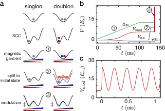
Figure S4: Experimental sequence. a Separate illustrations of the individual experimental steps for singly- and doubly-occupied double wells. The dots denote atoms in the $F\!=\!1$ manifold of ⁸⁷Rb in the $m_{F}\!=\!-1$ (blue), $m_{F}\!=\!0$ (gray) and $m_{F}\!=\!+1$ (red) state. The red and blue triangles illustrate the respective potential induced by the magnetic gradient. b Parameter ramps for the numbered steps in a. c Measured modulation lattice intensity, with sudden jump at $t\!=\!0$.

S.XIII.6 Experimental sequence for the $\mathbb{Z}_{2}$ two-site model

The experimental sequence for the data presented in Fig. 3 and 4 in the main text starts by loading atoms in the $\left|F\!=\!1,m_{F}\!=\!-1\right>$ state into a 3D optical lattice with lattice depths $V_{x,\mathrm{l}}\!=\!30(1)\,E_{r,\mathrm{l}}$, $V_{y}\!=\!35(1)\,E_{r,\mathrm{s}}$ and $V_{z}\!=\!50(2)\,E_{r,\mathrm{s}}$. These initial ramps are exponentially shaped and carried out in a time-segment of $50\,\textrm{ms}$ length. The $1/e$-time of the exponential ramp is $\tau\!=\!5\,$ms for the horizontal lattices ($x$, $y$) and $\tau_{z}\!=\!1.5\,$ms for the vertical lattice ($z$). This loading procedure was optimized for a maximal amount of doubly-occupied sites, while loading a negligible amount of tripply- and a small amount of singly-occupied sites. Later, each doubly-occupied site will realize a $\mathbb{Z}_{2}$ two-site model with both an $a$- and an $f$-particle. To create these distinguishable atoms, we use coherent spin-changing collisions (SCC) Widera et al. (2005) to transfer atom pairs to the $\left|F\!=\!1,m_{F}\!=\!\pm 1\right>$ states (Fig. S4a). To this end, we first apply a series of microwave-driven adiabatic passages to transfer the atoms to the $\left|F\!=\!1,m_{F}\!=\!0\right>$ state. Subsequently, the short lattice in $x$-direction was ramped up to $V_{x,\mathrm{s}}\!=\!40(1)\,E_{r,\mathrm{s}}$ within $15\,\textrm{ms}$ with a superlattice phase $\varphi_{\mathrm{SL}}$, such that both particles are localized to a single site of the double well. At the same time the lattice depths along the orthogonal directions are raised to $V_{y}\!=\!100(5)\,E_{r,\mathrm{s}}$ and $V_{z}\!=\!120(6)\,E_{r,\mathrm{s}}$ to further increase the on-site interaction energy. Finally, an adiabatic passage of microwave-mediated SCC was performed within $100\,$ms. Note, single atoms on a double well are not affected by SCC and remain in the $\left|F\!=\!1,m_{F}\!=\!0\right>$ state, which allows us to independently detect singly- and doubly-occupied sites. After the SCC sequence, the double-well sites are merged again in $15\,\textrm{ms}$ by adiabatically switching off $V_{x,\mathrm{s}}\!=\!0$. Then, a magnetic field gradient of $B^{\prime}/h\approx 5.9(3)\,\mathrm{kHz}/\lambda_{\mathrm{s}}$ was applied within $120\,\textrm{ms}$. Simultaneously, the modulation lattice is turned on to $V_{\mathrm{mod}}\!=\!6.0(1)\,E_{r,\mathrm{l}}$ and the superlattice phase ramped up to the final value. The initial state is prepared by ramping up $V_{x,\mathrm{s}}\!=\!9.50(1)\,E_{r,\mathrm{s}}$ in $10\,$ms as described above. Then, the modulation is started with a sudden jump ($50\,\upmu$s) of the modulation intensity to obtain the correct initial driving phase of $\phi\!=\!0$ (Fig. S4c). The modulation is performed with an amplitude of $A_{\mathrm{mod}}\!=\!9.0(1)\,E_{r,\mathrm{l}}$ around a mean value of $V_{\mathrm{mod}}^{(0)}\!=\!15.0(1)\,E_{r,\mathrm{l}}$ and a driving frequency of $\omega\!=\!2\pi\times 4320\,$Hz. The initial state evolves in this driven model, for different times $t$, approximating the time-dynamics in the $\mathbb{Z}_{2}$ two-site model. Subsequently, the tunneling dynamics was inhibited by rapidly increasing the potential barrier between the two sites $V_{x,\mathrm{s}}\!=\!40(1)\,E_{r,\mathrm{s}}$ in $50\,\upmu$s, followed by a site-resolved band-mapping detection in combination with a Stern-Gerlach species separation Sebby-Strabley et al. (2006); Fölling et al. (2007); Trotzky et al. (2008).

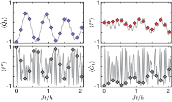
Figure S5: Time evolution for a single $\mathbb{Z}_{2}$ two-site model. Solid lines are the expectation values for the time evolution of the $\mathbb{Z}_{2}$ charge $\langle\hat{Q}_{1}\rangle$, the $\mathbb{Z}_{2}$ gauge field $\langle\hat{\tau}^{z}\rangle$, the $\mathbb{Z}_{2}$ electric field $\langle\hat{\tau}^{x}\rangle$, and the $\mathbb{Z}_{2}$ symmetry operator $\langle\hat{G}_{1}\rangle$. The parameters are identical to the ones used in Fig. 4. Note, the traces are for a single double well and not averaged over a distribution of tilts. Diamonds are stroboscopic time points.

S.XIV Numeric time evolution

The analysis of the effective Floquet model is compared to a full, time-dependent numerical analysis of the two-site two-particle model. We use formulation (S.16), which is very close to the experimental realization including the superlattice, magnetic gradient and first-order corrections to the Bose-Hubbard model.

We use the experimentally calibrated parameters $J^{\prime}$, $U$, $\Delta_{\mathrm{M}}$, $\Delta_{\mathrm{SL}}$, and $\omega$ together with calculated extended Bose-Hubbard parameters $\delta j$ and $u_{\mathrm{LR}}$ to perform a numerical time evolution. The time evolution is performed using the Trotter method by applying the quasi-static time evolution operator $\hat{U}_{n}\!=\!\exp\{-\mathrm{i}\,H(t_{n})\Delta t/\hbar\}$ for each time point $t_{n}\!=\!n\,\Delta t$ with $n\in\mathbb{N}$. The time step $\Delta t\!=\!2\pi/(s\omega)$ is chosen to subsample the driving frequency with $s\sim 50$. For the initial state $\left|\psi^{x}_{\mathrm{init}}\right>$, the groundstate of the configuration for the initial state preparation is chosen as explained above.

A single calculated time-trace shows strong oscillatory behavior (Fig. S5), which is not present in the stroboscopic calculation of the Floquet Hamiltonian and can be attributed to the micromotion. The micromotion is an additional dynamics with a period equal to the driving frequency.

The experimentally measured observables are averaged over many realizations of double wells. Due to inhomogeneities in the energy offsets between neighboring sites, the traces of individual double wells are different. We model these inhomogeneties with a Gaussian distribution of tilts as described in Eq. (S.14) with a standard deviation of $\Delta_{\sigma}$, extracted from the measurement of tunnel oscillations. From this distribution we randomly draw $1000$ tilt values and average the observables.

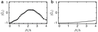
Figure S6: Symmetry breaking due to finite-frequency and extended Bose-Hubbard corrections. a The solid line is the time evolution according to the time-evolution operator (S.8) of the expectation value of the $\mathbb{Z}_{2}$ symmetry operator $\langle\hat{G}_{1}\rangle$ including the two lowest-order terms of the effective Floquet Hamiltonian (S.7). Diamonds show the stroboscopic dynamics of the full time-dependent Hamiltonian (3) from the main text for resonant driving at $\hbar\omega\!=\!\sqrt{U^{2}+4J^{2}}\!\approx\!1.04\,U$ and $U/J\!=\!7$. The gray line shows the ideal solution Eq. (6). The corresponding dynamics of $\langle\hat{Q}_{1}\rangle$ and $\langle\hat{\tau}^{z}\rangle$ are shown in Fig. S1. b Time evolution of the expectation value of the $\mathbb{Z}_{2}$ symmetry operator $\langle\hat{G}_{1}\rangle$ including additional terms from the extended Bose-Hubbard model with a strength $u_{\mathrm{LR}}\!=\!0.03\,J$ to the effective Floquet model in the infinite-frequency limit. For all calculations the initial state was $\left|\psi^{x}_{\mathrm{init}}\right>\!=\!(\left|1\right>+\left|2\right>)/\sqrt{2}$.

S.XV Symmetry-breaking correction terms in the experimental realization

It is essential for experimental realizations of LGTs that the underlying gauge symmetry is sufficiently conserved during the experiment. This puts high requirements on experimental implementations to suppress symmetry-breaking terms. In the presented scheme, we find two main sources for symmetry breaking: finite-frequency corrections to the effective Floquet Hamiltonian and first-order corrections to the Bose-Hubbard model.

The first-order correction to the Floquet Hamiltonian for finite-frequency drive was derived above [Eq. (S.7)]. The corrections contain diagonal detuning, correlated hopping and direct exchange coupling terms, which scale as $J^{2}/(\hbar\omega)$. The driving frequency is connected to the interaction energy in this realization. Therefore, the corrections can be reduced by either increasing the interaction energy or decreasing the tunnel coupling $J$. The effect on the $\mathbb{Z}_{2}$ symmetry is studied in Fig. S6a for $U/J\!=\!7$, similar to the experimental parameters, and an initial state in the $g_{1}\!=\!-1$ subsector.

The additional terms from the extended Bose-Hubbard model were introduced in Eq. (S.16) and are nearest-neighbor interactions, correlated tunneling and a direct exchange coupling. The terms scale with the square overlap of neighboring Wannier functions, $u_{\text{LR}}\!=\!g\int|w_{\mathrm{L}}(r)|^{2}|w_{\mathrm{R}}(r)|^{2}\,\mathrm{d}r^{3}$, and vanish therefore faster than the tunnel coupling $J$, when reducing the Wannier overlap. In Fig. S6b the correction terms were added to the infinite-frequency Floquet model with strength $u_{\mathrm{LR}}\!=\!0.03\,J$ and the time evolution of the expectation value of $\hat{G}$ was calculated numerically.

Both symmetry-breaking terms can be reduced by increasing the short period lattice potential depth, as the Wannier function overlap between neighboring sites reduces, while the on-site overlap and therefore the interaction energy increases. In Fig. S7, the relative scaling of the correction terms with $V_{x,\mathrm{s}}$ are shown. Note, to keep the ratio between the inter-double well tunneling rate $J_{i}$ and the tunneling rate $J$ constant for comparability, the long period lattice depth was scaled accordingly with $V_{x,\mathrm{l}}\propto\sqrt{V_{x,\mathrm{s}}}$.

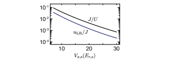
Figure S7: Suppressing the corrections. Scaling of the tight-binding parameters $J/U$ and $u_{\mathrm{LR}}/J$ with $V_{x,\mathrm{s}}$ and $V_{x,\mathrm{l}}\sim\sqrt{V_{x,\mathrm{s}}}$ for an initial ratio of $V_{x,\mathrm{s}}/V_{x,\mathrm{l}}=9.5/35$. This relative scaling keeps the ratio of the inter- to the intra-double well tunneling constant.

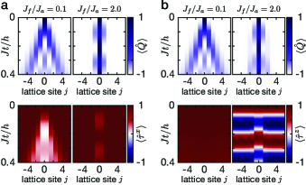
Figure S8: Numerical time evolution of a 1D $\mathbb{Z}_{2}$ chain with one matter particle. Dynamics of the matter particle and $\mathbb{Z}_{2}$ degrees-of-freedom for two different initial states calculated using exact diagonalization on a system with 13 sites based on Eq. (1). The matter particle is initially localized on site $j\!=\!0$. a All links are initialized in $\tau^{x}_{\langle j,j+1\rangle}\!=\!+1$. b All links are initialized in $\tau^{z}_{\langle j,j+1\rangle}\!=\!+1$.

S.XVI $\mathbb{Z}_{2}$ LGT in 1D

S.XVI.1 The ideal 1D model

The $\mathbb{Z}_{2}$ double well is a minimal two-site model, which consists of one link and a single matter particle. A direct generalization of this model arises when extending the double well to a chain by adding more links, an experimental scheme to realize such a system is introduced below. We discuss the dynamics for the resulting $\mathbb{Z}_{2}$ chain described by Eq. (1) in the main text in different regimes $J_{f}/J_{a}$ and for two initial states analogous to the ones used in the main text to study the two-site model. The dynamics of the system is analyzed by a calculation of the numerical time evolution with a Hamiltonian for $13$ sites. Initially, the matter particle is always in the center of the system labeled $j\!=\!0$.

We first start with an initial state, where all links are in the groundstate of the electric field operator $-\hat{\tau}^{x}_{\langle j,j+1\rangle}$. Therefore $\tau^{x}_{\langle j,j+1\rangle}\!=\!+1$ for all sites $j$. Together with the matter particle at site $j\!=\!0$, this leads to $g_{j}\!=\!+1$ for all $j\neq 0$ and a local static charge at $j\!=\!0$ described by $g_{0}\!=\!-1$. As $\hat{G}$ commutes with the Hamiltonian (1), the static charges $g_{j}$ are conserved. Thus, when the matter particle traverses a link its electric field value needs to change. This process is associated with an energy cost proportional to $J_{f}$. Figure S8a summarizes the result for two different regimes. In the regime $J_{f}\ll J_{a}$, the energy cost of flipping a traversed link, changing the value of $\tau^{x}$, is small and the matter particle can freely expand, which is clearly visible in the expectation value of $\hat{Q}_{j}$. The same cone shape is visible in the expectation value of the electric field operator $\langle\hat{\tau}^{x}\rangle$. Inside the cone $\langle\hat{\tau}^{x}\rangle\approx 0$ because the particle either traversed the link or not. In the opposite regime, where $J_{f}>J_{a}$, the energy cost for flipping $\tau^{x}$ is high, and also linearly increases with the number of traversed links. Therefore, the matter particle stays confined to the local static charge at site $j\!=\!0$.

Analog to the experiment on the two-site model, an initial state is examined, where each link is in an eigenstate of the gauge field operator $\hat{\tau}^{z}$. In this situation, instead of a single subsector a superposition of many subsectors is probed. We again investigate the two different regimes and present the results in Fig. S8b. In the regime $J_{f}\ll J_{a}$, the matter particle still expands freely, while we again observe confinement of the matter particle in the regime $J_{f}>J_{a}$. The expectation value of the electric field operator $\langle\hat{\tau}^{x}\rangle\!=\!0$ for all sites and times. The expectation value of the gauge field operator $\langle\hat{\tau}^{z}\rangle$, on the other hand, shows dynamics. This dynamics can be explained on the level of a single link prepared in one of the eigenstates of $\hat{\tau}^{z}$. The coupling $-J_{f}\hat{\tau}^{x}$ leads to Rabi oscillations between $\tau^{z}\!=\!\pm 1$. In the presence of the matter particle the Rabi oscillations are detuned, which leads to faster oscillations with a reduced amplitude.

S.XVI.2 1D model with super-sites

Super-site Hamiltonian — The $\mathbb{Z}_{2}$ double-well model is based on inter-species on-site interactions between $f$- and $a$-particles. Simply connecting two double-wells by introducing a joint site shared by both leads to an ambiguous situation: The $a$-particle can then no longer distinguish to which link the $f$-particles belong, unless different species $f$ and $f^{\prime}$ are used on alternating links.

To resolve this complication, the $\mathbb{Z}_{2}$ double wells can be connected via a tunnel coupling $J_{c}$ of the $a$-particle from the right site of the left double-well ($2j$) to the left site of the right double-well ($2j+1$). Hence, the individual building blocks remain functional. The resulting chain of coupled double-well building blocks can then be understood as a 1D model of super-sites at positions $j$. Each super-site consists of matter creation operators $\hat{a}_{j}^{\dagger}$ and $\hat{b}_{j}^{\dagger}$, describing the $a$-particles on sites $2j$ and $2j+1$, respectively. In this language, the super-sites are connected by a link with a gauge field $\hat{\tau}^{z}_{\langle j,j\pm 1\rangle}$. The corresponding Hamiltonian is

$$\hat{H}^{\mathrm{s}}_{\mathrm{1D}}= \sum\limits_{j}\left[-J^{\mathrm{s}}_{a}\,\hat{a}^{\dagger}_{j+1}\hat{\tau}^{z}_{\langle j,j+1\rangle}\hat{b}^{\phantom{\dagger}}_{j}-J^{\mathrm{s}}_{c}\,\hat{a}^{\dagger}_{j}\hat{b}^{\phantom{\dagger}}_{j}+\mathrm{h.c.}\right]$$

$$-\sum\limits_{j}J^{\mathrm{s}}_{f}\,\hat{\tau}^{x}_{\langle j,j+1\rangle}.$$ (S.17)

When replacing the $\mathbb{Z}_{2}$ charge by the super-site charge

$$\hat{Q}^{\mathrm{s}}_{j}=\mathrm{e}^{\mathrm{i}\pi(\hat{n}^{a}_{j}+\hat{n}^{b}_{j})},$$ (S.18)

which depends on the matter particle occupation on the super-site $\hat{n}^{s}_{j}=\hat{n}^{a}_{j}+\hat{n}^{b}_{j}$, then $\hat{H}_{\mathrm{1D},\,ab}$ is $\mathbb{Z}_{2}$ gauge-invariant with respect to the super-sites and commutes with the gauge transformation $[\hat{H}^{\mathrm{s}}_{\mathrm{1D}},\hat{G}^{\mathrm{s}}_{jb}]=0$ for all $j$.

Figure S9: Illustration of the super-site model. Each site in the 1D $\mathbb{Z}_{2}$ chain is replaced by a super-site with two physical sites $a$ and $b$. They are coupled by a tunneling rate $J^{\mathrm{s}}_{\mathrm{c}}$. The links between the super-sites have a $\mathbb{Z}_{2}$ degree-of-freedom and are realized by the building blocks.

Ideal model limit of the super-site Hamiltonian — The super-site Hamiltonian reduces to the 1D model Eq. (1) in the main text, if $J^{\mathrm{s}}_{c}\gg J^{\mathrm{s}}_{a}$. In this limit, each super-site forms an energetically lower (upper) orbital $\hat{h}_{j,\pm}=(\hat{a}_{j}\pm\hat{b}_{j})/\sqrt{2}$ with on-site energies described by $-J^{\mathrm{s}}_{c}(\hat{h}_{j,+}^{\dagger}\hat{h}_{j,+}-\hat{h}_{j,-}^{\dagger}\hat{h}_{j,-})=-J^{\mathrm{s}}_{c}(\hat{n}^{h}_{j,+}-\hat{n}^{h}_{j,-})$. Couplings between those higher and lower bands can be neglected in this limit $J^{\mathrm{s}}_{a}\ll J^{\mathrm{s}}_{c}$ and the effective Hamiltonian becomes

$$\hat{H}^{\mathrm{s}}_{\mathrm{1D}}= -J^{\mathrm{s}\star}_{a}\sum\limits_{j}\sum_{\mu=\pm}\mu\left[\,\hat{h}^{\dagger}_{j+1,\mu}\hat{\tau}^{z}_{\langle j,j+1\rangle}\hat{h}^{\phantom{\dagger}}_{j,\mu}+\mathrm{h.c.}\right]$$

$$-J^{\mathrm{s}}_{c}\sum\limits_{j}\left(\hat{n}^{h}_{j,+}-\hat{n}^{h}_{j,-}\right)$$

$$-J^{\mathrm{s}}_{f}\sum\limits_{j}\hat{\tau}^{x}_{\langle j,j+1\rangle},$$ (S.19)

where $J^{\mathrm{s}\star}_{a}=J^{\mathrm{s}}_{a}/2$. At low energies, or in properly prepared states, the higher band remains unoccupied, $\hat{n}^{h}_{j,-}=0$ for all $j$ and as a function of time. This yields a 1D $\mathbb{Z}_{2}$ LGT as discussed in the main text,

$$\hat{H}^{\mathrm{s}}_{\mathrm{1D}}= -J^{\mathrm{s}\star}_{a}\sum\limits_{j}\left[\,\hat{h}^{\dagger}_{j+1,+}\hat{\tau}^{z}_{\langle j,j+1\rangle}\hat{h}^{\phantom{\dagger}}_{j,+}+\mathrm{h.c.}\right]$$

$$-J^{\mathrm{s}}_{c}\sum\limits_{j}\hat{n}^{h}_{j,+}-J^{\mathrm{s}}_{f}\sum\limits_{j}\hat{\tau}^{x}_{\langle j,j+1\rangle}.$$ (S.20)

If Hubbard interactions $\hat{n}^{a}_{j}(\hat{n}^{a}_{j}-1)U_{a}/2$ and $\hat{n}^{b}_{j}(\hat{n}^{b}_{j}-1)U_{b}/2$ are present initially, which are weak compared to the super-site tunneling $U_{a,b}\ll|J^{\mathrm{s}}_{c}|$, they cannot cause significant mixing of the symmetric and anti-symmetric super-site orbitals. Projecting them to the lower band yields a new term

$$\hat{H}=\sum_{j}\frac{1}{2}U^{*}\hat{n}^{h}_{j,+}(\hat{n}^{h}_{j,+}-1)+\delta\mu\sum_{j}\hat{n}^{h}_{j,+}$$ (S.21)

with an effective Hubbard interaction $U^{\star}=(U_{a}+U_{b})/4$ and renormalization of the chemical potential by $\delta\mu=-(U_{a}+U_{b})/8$. Thus, if in addition to $U_{a,b}\ll|J_{c}|$ it also holds $|J^{\mathrm{s}}_{a}|\ll U^{\star}$, we can treat the resulting model by assuming that $\hat{h}_{j,+}$ are hard-core bosons.

Because the model in Eq. (S.17) has local $\mathbb{Z}_{2}$ gauge symmetries on the super-sites, the properties of its eigenstates are qualitatively similar to those of the simplified one-band model in Eq. (S.20), even if $J^{\mathrm{s}}_{c}$ is comparable to $J^{\mathrm{s}}_{a}$. To demonstrate this, we repeated the simulations from Fig. 1 in the main text, but in a more realistic super-site model. We compare cases where $J_{a}$ in the ideal model from the main text is equal to $J^{\mathrm{s}\star}_{a}$ in the super-site Hamiltonian. We find similar behavior for different values of the super-site coupling $J^{\mathrm{s}}_{c}$ (Fig. S10) after releasing a $\mathbb{Z}_{2}$ charge on the central super-site. Already for small values of the super-site coupling $J^{\mathrm{s}}_{c}=J^{\mathrm{s}}_{a}$ in the super-site model Eq. (S.17), we find a good quantitative agreement with the ideal 1D model introduced in Eq. (1) in the main text.

Floquet scheme — The super-site model above can be realized by a Floquet scheme. In the following we present one possible microscopic approach, as illustrated in Fig. S11, which is closely related to the proposal from Ref. Barbiero et al. (2019), using the same notations as in Eq. (S.17). On the double-well building blocks the processes are identical to the ones described in the main text, which we already implemented experimentally.

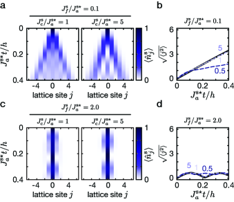
Figure S10: Numerical time evolution of the 1D $\mathbb{Z}_{2}$ super-site chain with one matter particle. Dynamics of the matter particle calculated using exact diagonalization of a system with 12 $\mathbb{Z}_{2}$ building blocks connected by 11 super-sites based on Eq. (S.17), with $J^{\mathrm{s}\star}_{a}=J^{\mathrm{s}}_{a}/2$. The initial state is a matter particle localized on site $j\!=\!0$ and all links are initialized in $\tau^{x}_{\langle j,j+1\rangle}\!=\!+1$. a Super-site occupation $n^{\mathrm{s}}_{j}$ in a regime with low electric field strength $J^{\mathrm{s}}_{f}/J^{\mathrm{s}\star}_{a}=0.1$ for different values of the super-site tunnel coupling $J^{\mathrm{s}}_{c}$. b Root-mean-square distance to the initial position $\sqrt{\left<j^{2}\right>}$. The values of $J^{\mathrm{s}}_{c}/J^{\mathrm{s}\star}_{a}$ are indicated next to the curves. A free expansion is observed already for $J^{\mathrm{s}}_{c}/J^{\mathrm{s}\star}_{a}\gtrsim 1$, which agrees well with the ideal evolution expected from the ideal 1D model captured by Eq. (1) in the main text (black thick line). c-d Results in the regime $J^{\mathrm{s}}_{f}/J^{\mathrm{s}\star}_{a}=2$ analogous to a-b.

We start from the following static Hamiltonian,

$$\hat{H}_{0}=-J^{0}_{f}\sum_{j}\hat{\tau}^{x}_{\langle j+1,j\rangle}+\frac{\Delta_{f}}{2}\sum_{j}\hat{\tau}^{z}_{\langle j+1,j\rangle}-J^{0}_{a}\sum_{j}\left(\hat{a}_{j+1}^{\dagger}\hat{b}_{j}+\mathrm{h.c.}\right)-J^{0}_{c}\sum_{j}\left(\hat{b}_{j}^{\dagger}\hat{a}_{j}+\mathrm{h.c.}\right)\\ +\Delta_{a}^{\prime}\sum_{j}\left[2j\hat{n}^{a}_{j}+(2j+1)\hat{n}^{b}_{j}\right]-\frac{\Delta_{a}}{2}\sum_{j}\left[\hat{n}^{a}_{j}-\hat{n}^{b}_{j}\right]+\frac{U}{2}\sum_{j}\left[(1-\hat{\tau}^{z}_{\langle j+1,j\rangle})\hat{n}^{b}_{j}+(1+\hat{\tau}^{z}_{\langle j+1,j\rangle})\hat{n}^{a}_{j+1}\right].$$ (S.22)

The first term corresponds to tunneling $J^{0}_{f}$ of the $f$-particles between the super-sites, which is initially suppressed by the gradient $\Delta_{f}$. The next two terms are bare tunnel couplings of the $a$-particles between and within the super-sites. They are initially suppressed by the following two terms: a linear gradient $\Delta_{a}^{\prime}$ and an alternating potential $\pm\Delta_{a}/2$ on the two inequivalent positions in the super-site. The last term corresponds to local inter-species Hubbard interactions between $a$ and $f$ particles on all sites.

To obtain the $\mathbb{Z}_{2}$ gauge invariant super-site model, we supplement $\hat{H}_{0}$ by the following driving terms,

$$\hat{H}_{\omega}(t)=\bigl{(}V_{\omega}^{a}\cos(\omega t)+V_{2\omega}^{a}\cos(2\omega t)\bigr{)}\sum_{j}\left[2j\hat{n}^{a}_{j}+(2j+1)\hat{n}^{b}_{j}\right]+\frac{\Delta_{f}^{\omega}}{2}\cos(\omega t)\sum_{j}\hat{\tau}^{z}_{\langle j+1,j\rangle}\\ -\biggl{(}\frac{\Delta_{a}^{\omega}}{2}\cos(\omega t)+\frac{\Delta_{a}^{2\omega}}{2}\cos(2\omega t)\biggr{)}\sum_{j}\left[\hat{n}^{a}_{j}-\hat{n}^{b}_{j}\right],$$ (S.23)

which will be used to restore tunnel couplings of the $a$- and $f$-particles. The first term corresponds to a modulated linear gradient seen by the $a$-particles. The other two terms are modulated alternating potentials seen by the $f$- and $a$-particles, respectively. The modulations at two frequencies $\omega$ and $2\omega$ are used to control both the amplitude and phase of the resulting effective Floquet Hamiltonian, see Refs. Barbiero et al. (2019); Görg et al. (2019).

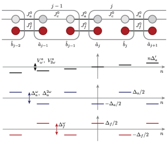
Figure S11: Floquet implementation of the super-site model. The super-sites are illustrated by the gray boxes. They consist of $a$ and $b$ sites, which are separately illustrated for $a$- and $f$-particles. The super-site tunnel coupling for the $a$-particles is $J^{0}_{c}$ and assumed to be negligible for the $f$-particles. The $a$-particles are exposed to a linear potential $n\Delta^{\prime}_{a}/2$, which is modulated by $\omega$ and $2\omega$ with a strength $V_{\omega}^{a}$ and $V_{2\omega}^{a}$. In addition, they experience a staggered potential $\pm\Delta_{a}$ between neighboring sites, which is also modulated by $\omega$ and $2\omega$ with the strength $\Delta^{\omega}_{a}$ and $\Delta^{2\omega}_{a}$. The $f$-particles experience an opposite staggered potential with $\Delta_{f}$. This potential is modulated with frequency $\omega$ and amplitude $\Delta^{\omega}_{f}$.

Following the scheme proposed in Ref. Barbiero et al. (2019), we require the following resonance conditions:

$$\hbar\omega=\Delta_{f} =U$$ (S.24)

$$\Delta_{a}=\Delta_{a}^{\prime} =U/2$$ (S.25)

$$\Delta_{a}^{2\omega}=V_{2\omega}^{a} \equiv V_{2\omega}^{x}/2$$ (S.26)

$$V_{\omega}^{a}-\Delta_{a}^{\omega}=\Delta_{f}^{\omega} \equiv V_{\omega}^{y}$$ (S.27)

$$V_{\omega}^{a}+\Delta_{a}^{\omega} \equiv V_{\omega}^{x}.$$ (S.28)

The last three lines include the three amplitudes $V_{2\omega}^{x}$, $V_{\omega}^{x}$ and $V_{\omega}^{y}$ which are fixed by

$$x^{(1)}=V_{\omega}^{x}/(\hbar\omega) \simeq 1.71$$ (S.29)

$$x^{(2)}=V_{2\omega}^{x}/(\hbar\omega) \simeq 1.05$$ (S.30)

$$y^{(1)}=V_{\omega}^{y}/(\hbar\omega) \simeq 1.84$$ (S.31)

These are solutions to $\mathcal{J}_{0}(y^{(1)})=\mathcal{J}_{2}(y^{(1)})$ and $\lambda_{0}=\lambda_{1}=\lambda_{2}\equiv\lambda_{012}$ where $\lambda_{n}=\sum_{\ell=-\infty}^{\infty}\mathcal{J}_{n-2\ell}(x^{(1)})\mathcal{J}_{\ell}(x^{(2)}/2)$.

In the large frequency limit, and under the above conditions, the effective Floquet Hamiltonian becomes Goldman et al. (2015)

$$\hat{H}_{\rm eff}=-J^{0}_{f}\sum_{j}\hat{\tau}^{x}_{\langle j+1,j\rangle}\hat{\Lambda}^{y}_{\langle j+1,j\rangle}-J^{0}_{c}\sum_{j}\lambda^{x}\left(\hat{a}^{\dagger}_{j}\hat{b}_{j}+\mathrm{h.c.}\right)\\ -J^{0}_{a}\sum_{j}\lambda^{y}\left(\hat{a}_{j+1}^{\dagger}\hat{\tau}^{z}_{\langle j+1,j\rangle}\hat{b}_{j}+\mathrm{h.c.}\right).$$ (S.32)

The renormalization of tunneling amplitudes is given by

$$\hat{\Lambda}^{y}_{\langle j+1,j\rangle}=\frac{1}{2}\left(1-(-1)^{\hat{n}^{a}_{j+1}+\hat{n}^{b}_{j}}\right)\mathcal{J}_{0}(y^{(1)})\\ +\frac{1}{2}\left(1+(-1)^{\hat{n}^{a}_{j+1}+\hat{n}^{b}_{j}}\right)\mathcal{J}_{1}(y^{(1)}),$$ (S.33)

$\lambda^{x}=\lambda_{012}\simeq 0.37$ and $\lambda^{y}=\mathcal{J}_{1}(y^{(1)})\simeq 0.58$.

One easily confirms that Hamiltonian (S.32) is $\mathbb{Z}_{2}$ gauge invariant if the super-site gauge operator is used,

$$\hat{G}_{j,ab}=\hat{Q}_{j,ab}\hat{\tau}^{x}_{\langle j-1,j\rangle}\hat{\tau}^{x}_{\langle j,j+1\rangle}.$$ (S.34)

The effective Hamiltonian (S.32) is similar to the super-site model in Eq. (S.17), except for the fact that the renormalization of the $f$-particle tunneling, $\hat{\Lambda}^{y}_{\langle j+1,j\rangle}$, is operator-valued and depends on the $\mathbb{Z}_{2}$ charges on the adjacent sites. This is not expected to change the physics of the model. If required, two-frequency driving can also be used for the $f$-particles to obtain a situation where $\hat{\Lambda}^{y}\to\Lambda^{y}$ becomes a $\mathbb{C}$ number.

To illustrate the accuracy of our Floquet scheme, in Fig. S12 we repeat our calculations from Fig. S10 starting from the microscopic model. The parameters in Eqs. (S.22), (S.23) are chosen such that the effective couplings in Eq. (S.32) correspond to the parameters we used in the super-site model Eq. (S.17). For $U=10J^{0}_{a}$ in the microscopic Hamiltonian, we find that the $\mathbb{Z}_{2}$ gauge invariance remains valid for long times and the observed dynamics is similar to our expectation from the super-site model. In Fig. S13 we also performed simulations starting from an initial state with two fermionic $\mathbb{Z}_{2}$ charges $a$ located next to each other, connected by a $\mathbb{Z}_{2}$ electric field line. In this case, too, the gauge invariance of the model remains intact for long times. This establishes the proposed Floquet scheme as a realistic method to implement and realize dynamics in models with local $\mathbb{Z}_{2}$ gauge constraints.

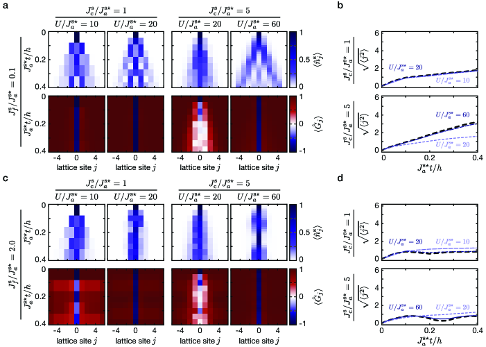
Figure S12: Numerical time evolution of the full time-dependent model with one particle. Dynamics of the matter particle calculated by numerically solving the time-dependent model according to Eqs. (S.22) and (S.23), fulfilling the resonance conditions Eqs. (S.24) – (S.31) and setting $J_{a}^{0}=2J_{a}^{\mathrm{s}\star}/\mathcal{J}_{1}(y^{(1)})$, $J_{c}^{0}=J_{c}/\lambda^{x}$ and $J_{f}^{0}=J_{f}/\mathcal{J}_{1}(y^{(1)})$. The system consists of 10 $\mathbb{Z}_{2}$ building blocks and 9 super-sites. The edges of the 1D chain have therefore only a single site. The initial state is a matter particle localized on site $j\!=\!0$ and all links are initialized in $\tau^{x}_{\langle j,j+1\rangle}\!=\!+1$. a Matter particle dynamics and expectation value of the local symmetry operator $\langle\hat{G}_{j}\rangle$ in a regime with low electric field strength $J^{\mathrm{s}}_{f}/J^{\mathrm{s}\star}_{a}=0.1$ for different inter-species interaction energies $U$. b Root-mean-square distance to the initial position $\sqrt{\left<j^{2}\right>}$ of the matter particle dynamics from a in comparison to the high-frequency limit. The results in the high-frequency limit are shown by thick dashed black lines. c-d Results in the regime $J^{\mathrm{s}}_{f}/J^{\mathrm{s}\star}_{a}=2$ analogous to a-b.

—

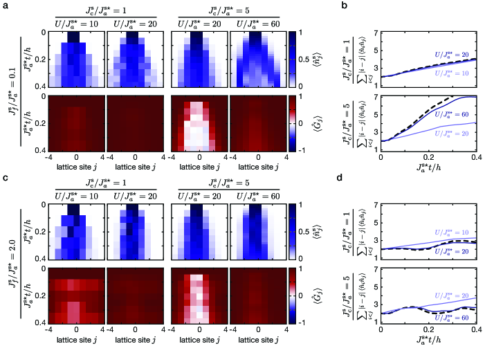
Figure S13: Numerical time evolution of the full time-dependent model with two particles. Dynamics of two matter particles calculated by numerically solving the time-dependent model according to Eqs. (S.22) and (S.23), fulfilling the resonance conditions Eqs. (S.24) – (S.31) and setting $J_{a}^{0}=2J_{a}^{\mathrm{s}\star}/\mathcal{J}_{1}(y^{(1)})$, $J_{c}^{0}=J_{c}/\lambda^{x}$ and $J_{f}^{0}=J_{f}/\mathcal{J}_{1}(y^{(1)})$. The system consists of 8 $\mathbb{Z}_{2}$ building blocks and 9 super-sites. The system’s edge is therefore a super-site. The initial state is a matter particle localized on site $j\!=\!0$ and a second matter particle at site $j\!=\!-1$. The link between the two sites is $\tau^{x}_{\langle-1,0\rangle}\!=\!-1$. All other links are initialized in $\tau^{x}_{\langle j,j+1\rangle}\!=\!+1$. a Matter particle dynamics and expectation value of the local symmetry operator $\langle\hat{G}_{j}\rangle$ in a regime with low electric field strength $J^{\mathrm{s}}_{f}/J^{\mathrm{s}\star}_{a}=0.1$ for different inter-species interaction energies $U$. b Time evolution of the distance between the two particles measured by $\sum_{i<j}|i-j|\langle\hat{n}_{i}\hat{n}_{j}\rangle$ for the data shown in a, in comparison to the high frequency-limit. The results in the high-frequency limit are shown by thick black lines. c-d Results in the regime $J^{\mathrm{s}}_{f}/J^{\mathrm{s}\star}_{a}=2$ analogous to a-b.

References

- Wilson (1974) Kenneth G. Wilson, “Confinement of quarks,” Phys. Rev. D 10, 2445–2459 (1974).
- Kogut (1979) John B. Kogut, “An introduction to lattice gauge theory and spin systems,” Rev. Mod. Phys. 51, 659–713 (1979).
- Wen (2004) Xiao-Gang Wen, Quantum Field Theory of Many-body Systems (Oxford University Press, 2004).
- Levin and Wen (2005) Michael Levin and Xiao-Gang Wen, “Colloquium: Photons and electrons as emergent phenomena,” Rev. Mod. Phys. 77, 871–879 (2005).
- Lee et al. (2006) Patrick A. Lee, Naoto Nagaosa, and Xiao-Gang Wen, “Doping a Mott Insulator: Physics of High Temperature Superconductivity,” Rev. Mod. Phys. 78, 17–85 (2006).
- Ichinose and Matsui (2014) Ikuo Ichinose and Tetsuo Matsui, “Lattice gauge theory for condensed matter physics: ferromagnetic superconductivity as its example,” Mod. Phys. Lett. B 28, 1430012 (2014).
- Aoki et al. (2017) S. Aoki, Y. Aoki, D. Bečirević, C. Bernard, T. Blum, G. Colangelo, M. Della Morte, P. Dimopoulos, S. Dürr, H. Fukaya, M. Golterman, Steven Gottlieb, S. Hashimoto, U. M. Heller, R. Horsley, A. Jüttner, T. Kaneko, L. Lellouch, H. Leutwyler, C.-J. D. Lin, V. Lubicz, E. Lunghi, R. Mawhinney, T. Onogi, C. Pena, C. T. Sachrajda, S. R. Sharpe, S. Simula, R. Sommer, A. Vladikas, U. Wenger, and H. Wittig, “Review of lattice results concerning low-energy particle physics,” Eur. Phys. J. C 77, 112 (2017).
- Troyer and Wiese (2005) Matthias Troyer and Uwe-Jens Wiese, “Computational Complexity and Fundamental Limitations to Fermionic Quantum Monte Carlo Simulations,” Phys. Rev. Lett. 94, 170201 (2005).
- Alford et al. (2008) Mark G. Alford, Andreas Schmitt, Krishna Rajagopal, and Thomas Schäfer, “Color superconductivity in dense quark matter,” Rev. Mod. Phys. 80, 1455–1515 (2008).
- Buyens et al. (2016) Boye Buyens, Frank Verstraete, and Karel Van Acoleyen, “Hamiltonian simulation of the Schwinger model at finite temperature,” Phys. Rev. D 94, 085018 (2016).
- Bañuls et al. (2017) Mari-Carmen Bañuls, Krzysztof Cichy, J. Ignacio Cirac, Karl Jansen, Stefan Kühn, and Hana Saito, “Towards overcoming the Monte Carlo sign problem with tensor networks,” EPJ Web Conf. 137, 04001 (2017).
- Silvi et al. (2017) Pietro Silvi, Enrique Rico, Marcello Dalmonte, Ferdinand Tschirsich, and Simone Montangero, “Finite-density phase diagram of a non-abelian lattice gauge theory with tensor networks,” Quantum 1, 9 (2017).
- Gazit et al. (2017) Snir Gazit, Mohit Randeria, and Ashvin Vishwanath, “Emergent Dirac fermions and broken symmetries in confined and deconfined phases of gauge theories,” Nat. Phys. 13, 484–490 (2017).
- Weimer et al. (2010) Hendrik Weimer, Markus Müller, Igor Lesanovsky, Peter Zoller, and Hans Peter Büchler, “A Rydberg quantum simulator,” Nat. Phys. 6, 382–388 (2010).
- Blatt and Roos (2012) Rainer Blatt and Christian F. Roos, “Quantum simulations with trapped ions,” Nat. Phys. 8, 277–284 (2012).
- Gross and Bloch (2017) Christian Gross and Immanuel Bloch, “Quantum simulations with ultracold atoms in optical lattices,” Science 357, 995–1001 (2017).
- Romero et al. (2017) Guillermo Romero, Enrique Solano, and Lucas Lamata, “Quantum simulations with photons and polaritons,” (2017) Chap. Quantum Simulations with Circuit Quantum Electrodynamics, pp. 153–180.
- Tagliacozzo et al. (2013) Luca Tagliacozzo, Alessio Celi, Alejandro Zamora, and Maciej Lewenstein, “Optical abelian lattice gauge theories,” Ann. Phys. (New York) 330, 160–191 (2013).
- Wiese (2013) Uwe-Jens Wiese, “Ultracold quantum gases and lattice systems: quantum simulation of lattice gauge theories,” Ann. Phys. (Berlin) 525, 777–796 (2013).
- Zohar et al. (2015) Erez Zohar, J. Ignacio Cirac, and Benni Reznik, “Quantum simulations of lattice gauge theories using ultracold atoms in optical lattices,” Rep. Prog. Phys. 79, 014401 (2015).
- Dalmonte and Montangero (2016) Marcello Dalmonte and Simone Montangero, “Lattice gauge theory simulations in the quantum information era,” Contemp. Phys. 57, 388–412 (2016).
- Notarnicola et al. (2015) Simone Notarnicola, Elisa Ercolessi, Paolo Facchi, Giuseppe Marmo, Saverio Pascazio, and Francesco V. Pepe, “Discrete Abelian gauge theories for quantum simulations of QED,” J. Phys. A Math. Theor. 48, 30FT01 (2015).
- Kasper et al. (2017) Valentin Kasper, Florian Hebenstreit, Fred Jendrzejewski, Markus K. Oberthaler, and Jürgen Berges, “Implementing quantum electrodynamics with ultracold atomic systems,” New J. Phys. 19, 023030 (2017).
- Kuno et al. (2017) Yoshihito Kuno, Shinya Sakane, Kenichi Kasamatsu, Ikuo Ichinose, and Tetsuo Matsui, “Quantum simulation of ()-dimensional gauge-higgs model on a lattice by cold Bose gases,” Phys. Rev. D 95, 094507 (2017).
- Zhang et al. (2018) Jin Zhang, Judah Unmuth-Yockey, Johannes Zeiher, Alexei Bazavov, Shan-Wen Tsai, and Yannick Meurice, “Quantum simulation of the universal features of the polyakov loop,” Phys. Rev. Lett. 121, 223201 (2018).
- Aidelsburger et al. (2018) Monika Aidelsburger, Sylvain Nascimbène, and Nathan Goldman, “Artificial gauge fields in materials and engineered systems,” C. R. Physique 19, 394–432 (2018).
- Clark et al. (2018) Logan W. Clark, Brandon M. Anderson, Lei Feng, Anita Gaj, Kathryn Levin, and Cheng Chin, “Observation of density-dependent gauge fields in a bose-einstein condensate based on micromotion control in a shaken two-dimensional lattice,” Phys. Rev. Lett. 121, 030402 (2018).
- Anderlini et al. (2007) Marco Anderlini, Patricia J. Lee, Benjamin L. Brown, Jennifer Sebby-Strabley, William D. Phillips, and J. V. Porto, “Controlled exchange interaction between pairs of neutral atoms in an optical lattice,” Nature 448–456, 452 (2007).
- Trotzky et al. (2008) Stefan Trotzky, Patrick Cheinet, Simon Fölling, Michael Feld, Ute Schnorrberger, Ana Maria Rey, Anatoli Polkovnikov, Eugene A. Demler, Mikhail D. Lukin, and Immanuel Bloch, “Time-Resolved Observation and Control of Superexchange Interactions with Ultracold Atoms in Optical Lattices,” Science 319, 295–299 (2008).
- Dai et al. (2017) Han-Ning Dai, Bing Yang, Andreas Reingruber, Hui Sun, Xiao-Fan Xu, Yu-Ao Chen, Zhen-Sheng Yuan, and Jian-Wei Pan, “Four-body ring-exchange interactions and anyonic statistics within a minimal toric-code Hamiltonian,” Nat. Phys. 13, 1195–1200 (2017).
- Klco et al. (2018) Natalie Klco, Eugene F. Dumitrescu, Alex J. McCaskey, Titus D. Morris, Raphael C. Pooser, Mikel Sanz, Enrique Solano, Pavel Lougovski, and Martin J. Savage, “Quantum-classical computation of schwinger model dynamics using quantum computers,” Phys. Rev. A 98, 032331 (2018).
- Martinez et al. (2016) Esteban A. Martinez, Christine A. Muschik, Philipp Schindler, Daniel Nigg, Alexander Erhard, Markus Heyl, Philipp Hauke, Marcello Dalmonte, Thomas Monz, Peter Zoller, and Rainer Blatt, “Real-time dynamics of lattice gauge theories with a few-qubit quantum computer,” Nature 534, 516–519 (2016).
- Barbiero et al. (2019) Luca Barbiero, Christian Schweizer, Monika Aidelsburger, Eugene Demler, Nathan Goldman, and Fabian Grusdt, “Coupling ultracold matter to dynamical gauge fields in optical lattices: From flux attachment to lattice gauge theories,” Science Advances 5 (2019), 10.1126/sciadv.aav7444.
- Zohar et al. (2017) Erez Zohar, Alessandro Farace, Benni Reznik, and J. Ignacio Cirac, “Digital quantum simulation of lattice gauge theories with dynamical fermionic matter,” Phys. Rev. Lett. 118, 070501 (2017).
- Horn et al. (1979) David Horn, Marvin Weinstein, and Shimon Yankielowicz, “Hamiltonian approach to lattice gauge theories,” Phys. Rev. D 19, 3715–3731 (1979).
- Ju and Balents (2013) Hyejin Ju and Leon Balents, “Finite-size effects in the spin liquid on the kagome lattice,” Phys. Rev. B 87, 195109 (2013).
- González-Cuadra et al. (2019) Daniel González-Cuadra, Alexandre Dauphin, Przemyslaw R. Grzybowski, Maciej Lewenstein, and Alejandro Bermudez, “Symmetry-Breaking Topological Insulator in the Bose-Hubbard Model ,” Phys. Rev. B 99, 045139 (2019).
- Kitaev (2003) Alexei Y. Kitaev, “Fault-tolerant quantum computation by anyons,” Ann. Phys. (New York) 303, 2–30 (2003).
- Keilmann et al. (2011) Tassilo Keilmann, Simon Lanzmich, Ian McCulloch, and Marco Roncaglia, “Statistically induced phase transitions and anyons in 1d optical lattices,” Nature Commun. 2, 361 (2011).
- Greschner and Santos (2015) Sebastian Greschner and Luis Santos, “Anyon hubbard model in one-dimensional optical lattices,” Phys. Rev. Lett. 115, 053002 (2015).
- Bermudez and Porras (2015) Alejandro Bermudez and Diego Porras, “Interaction-dependent photon-assisted tunneling in optical lattices: a quantum simulator of strongly-correlated electrons and dynamical gauge fields,” New. J. Phys. 17, 103021 (2015).
- Sträter et al. (2016) Christoph Sträter, Shashi C. L. Srivastava, and André Eckardt, “Floquet realization and signatures of one-dimensional anyons in an optical lattice,” Phys. Rev. Lett. 117, 205303 (2016).
- Goldman et al. (2015) Nathan Goldman, Jean Dalibard, Monika Aidelsburger, and Nigel R. Cooper, “Periodically driven quantum matter: The case of resonant modulations,” Phys. Rev. A 91, 033632 (2015).
- Goldman and Dalibard (2014) Nathan Goldman and Jean Dalibard, “Periodically driven quantum systems: Effective hamiltonians and engineered gauge fields,” Phys. Rev. X 4, 031027 (2014).
- Bukov et al. (2015) Marin Bukov, Luca D’Alessio, and Anatoli Polkovnikov, “Universal high-frequency behavior of periodically driven systems: from dynamical stabilization to Floquet engineering,” Adv. Phys. 64, 139–226 (2015).
- Eckardt (2017) André Eckardt, “Colloquium: Atomic quantum gases in periodically driven optical lattices,” Rev. Mod. Phys. 89, 011004 (2017).
- Ma et al. (2011) Ruichao Ma, M. Eric Tai, Philipp M. Preiss, Waseem S. Bakr, Jonathan Simon, and Markus Greiner, “Photon-Assisted Tunneling in a Biased Strongly Correlated Bose Gas,” Phys. Rev. Lett. 107, 095301 (2011).
- Chen et al. (2011) Yu-Ao Chen, Sylvain Nascimbène, Monika Aidelsburger, Marcos Atala, Stefan Trotzky, and Immanuel Bloch, “Controlling correlated tunneling and superexchange interactions with ac-driven optical lattices,” Phys. Rev. Lett. 107, 210405 (2011).
- Meinert et al. (2016) Florian Meinert, Manfred J. Mark, Katharina Lauber, Andrew J. Daley, and Hanns-Christoph Nägerl, “Floquet Engineering of Correlated Tunneling in the Bose-Hubbard Model with Ultracold Atoms,” Phys. Rev. Lett. 116, 205301 (2016).
- Görg et al. (2019) Frederik Görg, Kilian Sandholzer, Joaquín Minguzzi, Rémi Desbuquois, Michael Messer, and Tilman Esslinger, “Realization of density-dependent Peierls phases to engineer quantized gauge fields coupled to ultracold matter,” Nat. Phys. 15, 1–7 (2019).
- Keay et al. (1995) Brian J. Keay, Stefan Zeuner, S. James Allen, Kevin D. Maranowski, Art C. Gossard, Uddalak Bhattacharya, and Marc J. W. Rodwell, “Dynamic Localization, Absolute Negative Conductance, and Stimulated, Multiphoton Emission in Sequential Resonant Tunneling Semiconductor Superlattices,” Phys. Rev. Lett. 75, 4102–4105 (1995).
- Lignier et al. (2007) Hans Lignier, Carlo Sias, Donatella Ciampini, Yeshpal Singh, Alessandro Zenesini, Olivier Morsch, and Ennio Arimondo, “Dynamical control of matter-wave tunneling in periodic potentials,” Phys. Rev. Lett. 99, 220403 (2007).
- Sias et al. (2008) Carlo Sias, Hans Lignier, Yeshpal Singh, Alessandro Zenesini, Donatella Ciampini, Olivier Morsch, and Ennio Arimondo, “Observation of Photon-Assisted Tunneling in Optical Lattices,” Phys. Rev. Lett. 100, 63 (2008).
- Mukherjee et al. (2015) Sebabrata Mukherjee, Alexander Spracklen, Debaditya Choudhury, Nathan Goldman, Patrik Öhberg, Erika Andersson, and Robert R. Thomson, “Modulation-assisted tunneling in laser-fabricated photonic Wannier–Stark ladders,” New J. Phys. 17, 115002 (2015).
- Scarola and Das Sarma (2005) Vito W. Scarola and Sankar Das Sarma, “Quantum phases of the extended bose-hubbard hamiltonian: Possibility of a supersolid state of cold atoms in optical lattices,” Phys. Rev. Lett. 95, 033003 (2005).
- Banerjee et al. (2013) Debasish Banerjee, Michael Bögli, Marcello Dalmonte, Enrique Rico, Pascal Stebler, Uwe-Jens Wiese, and Peter Zoller, “Atomic quantum simulation of and non-abelian lattice gauge theories,” Phys. Rev. Lett. 110, 125303 (2013).
- Kühn et al. (2014) Stefan Kühn, J. Ignacio Cirac, and Mari-Carmen Bañuls, “Quantum simulation of the schwinger model: A study of feasibility,” Phys. Rev. A 90, 042305 (2014).
Supplementary Information for:

References

- Goldman et al. (2015) N. Goldman, J. Dalibard, M. Aidelsburger, and N. R. Cooper, Phys. Rev. A 91, 033632 (2015).
- Goldman and Dalibard (2014) N. Goldman and J. Dalibard, Phys. Rev. X 4, 031027 (2014).
- Sebby-Strabley et al. (2006) J. Sebby-Strabley, M. Anderlini, P. S. Jessen, and J. V. Porto, Phys. Rev. A 73, 033605 (2006).
- Fölling et al. (2007) S. Fölling, S. Trotzky, P. Cheinet, M. Feld, R. Saers, A. Widera, T. Müller, and I. Bloch, Nature 448, 1029 (2007).
- Scarola and Das Sarma (2005) V. W. Scarola and S. Das Sarma, Phys. Rev. Lett. 95, 033003 (2005).
- Widera et al. (2005) A. Widera, F. Gerbier, S. Fölling, T. Gericke, O. Mandel, and I. Bloch, Phys. Rev. Lett. 95, 190405 (2005).
- Trotzky et al. (2008) S. Trotzky, P. Cheinet, S. Fölling, M. Feld, U. Schnorrberger, A. M. Rey, A. Polkovnikov, E. A. Demler, M. D. Lukin, and I. Bloch, Science 319, 295 (2008).
- Barbiero et al. (2019) L. Barbiero, C. Schweizer, M. Aidelsburger, E. Demler, N. Goldman, and F. Grusdt, Science Advances 5 (2019), 10.1126/sciadv.aav7444.
- Görg et al. (2019) F. Görg, K. Sandholzer, J. Minguzzi, R. Desbuquois, M. Messer, and T. Esslinger, Nat. Phys. 15, 1 (2019).