Spectral Graph Analysis: A Unified Explanation and Modern Perspectives

Abstract

Complex networks or graphs are ubiquitous in sciences and engineering: biological networks, brain networks, transportation networks, social networks, and the World Wide Web, to name a few. Spectral graph theory provides a set of useful techniques and models for understanding ‘patterns of interconnectedness’ in a graph. Our prime focus in this paper is on the following question: Is there a unified explanation and description of the fundamental spectral graph methods? There are at least two reasons to be interested in this question. Firstly, to gain a much deeper and refined understanding of the basic foundational principles, and secondly, to derive rich consequences with practical significance for algorithm design. However, despite half a century of research, this question remains one of the most formidable open issues, if not the core problem in modern network science. The achievement of this paper is to take a step towards answering this question by discovering a simple, yet universal statistical logic of spectral graph analysis. The prescribed viewpoint appears to be good enough to accommodate almost all existing spectral graph techniques as a consequence of just one single formalism and algorithm.

1 Introduction

How can we efficiently represent a graph to characterize its intrinsic structure, is the “Holy-Grail” question that every graph-analyst wrestles with. Spectral graph theory provides an elegant framework and a formal mathematical language to address this key question, which has produced impressive results across a range of application domains including computer vision, neuroimaging, web search, smart grid, social network, recommender systems, high-dimensional modeling, and many others. Over the past few decades, researchers have made dramatic strides toward developing a suite of spectral graph analysis techniques (e.g., Laplacian, Modularity, Diffusion map, regularized Laplacian, Google PageRank model) with increasing sophistication and specialization. However, no single algorithm can be regarded as a panacea for dealing with the evolving complexities of modern graphs. Therefore, the most important and pressing question for the field today appears to be whether we can develop a unifying language to establish “bridges” between a body of heavily-used spectral graph analysis techniques, and thus provide logically connected means for reaching different ends. Undoubtedly, any such formulation would be of great theoretical significance and practical value, that will ultimately provide the applied data scientists clear guidance and a systematic strategy for selecting the proper spectral tools to arrive at a confident conclusion.

To that end, this work attempts to unify the theories of spectral graph analysis, embracing the existing paradigm by purely statistical means. Another benefit of this new viewpoint is that it provides surprising insights into the design of fast and scalable algorithms for large graphs, which are otherwise hard to guess using previous understanding.

1.1 Spectral Graph Analysis: A Practitioner’s Guide

The way spectral graph analysis is currently taught and practiced can be summarized as follows (also known as spectral heuristics[1, 2]):

1. Let $\mathcal{G}=(V,E)$ denotes a (possibly weighted) undirected graph with a finite set of vertices $|V|=n$, and a set of edges $E$. Represent the graph using weighted adjacency matrix $A$ where $A(x,y;\mathcal{G})=w_{xy}$ if the nodes $x$ and $y$ are connected by an edge and $0$ otherwise; weights are non-negative and symmetric. The degrees of the vertices are defined as ${\bm{d}}=A{\mathbf{1}}_{n}$ and $D={\rm diag}(d_{1},\ldots,d_{n})\in{\mathbb{R}}^{n\times n}$.

2. Define “suitable” spectral graph matrix (also known as graph “shift” operator). Most popular and successful ones are listed below:

   • $\mathcal{L}=D^{-1/2}AD^{-1/2}$     Chung (1997)[3].

   • $\mathcal{B}=A\,-\,N^{-1}{\bm{d}}{\bm{d}}^{T}$     Newman (2006)[4].

   • $\mathcal{T}=D^{-1}A$     Coifman and Lafon (2006)[5].

   • Type-I Reg. $\mathcal{L}_{\tau}=$ $D_{\tau}^{-1/2}A\,D_{\tau}^{-1/2}$      Chaudhuri et al. (2012)[6].

   • Type-II Reg. $\mathcal{L}_{\tau}=D_{\tau}^{-1/2}\,A_{\tau}\,D_{\tau}^{-1/2}$   Amini et al. (2013)[7].

   • Google’s PageRank $\mathcal{T}_{\alpha}=\alpha D^{-1}A+(1-\alpha)F$   Brin and Page (1999)[8].

   where $\tau,\alpha>0$ regularization parameters, $A_{\tau}=A+(\tau/n){\bf 1}{\bf 1}^{T}$, $D_{\tau}$ is a diagonal matrix with elements $A_{\tau}{\mathbf{1}}_{n}$, $F\in{\mathbb{R}}^{n\times n}$ with all entries $1/n$, and $N={\rm Vol}(\mathcal{G})=\sum_{x,y}A(x,y)$.

3. Perform spectral decomposition of the matrix selected at step 2, whose eigenvectors form an orthogonal basis of ${\mathbb{R}}^{n}$. Spectral graph theory seeks to understand the interesting structure of a graph by using leading nontrivial eigenvectors and eigenvalues, first recognized by Fiedler (1973)[9], which provide the basis for performing harmonic analysis on graphs.

4. Compute graph Fourier transform (GFT) by expanding functions defined over the vertices of a graph as a linear combination of the selected eigenbasis (from step 3) and carry out learning tasks such as regression, clustering, classification, smoothing, kriging, etc.

1.2 Motivating Questions: “Algorithm of Algorithms”

The theory and practice of graph data analysis remain very much unsystematic due to the paucity of attention thus far devoted to their foundational issues; the diversity of poorly related graph learning algorithms attests to this fact. Graph signal processing engineers are often left bewildered by the vastness of the existing literature and hugely diverse zoo of methods (developed by the machine learning community, applied harmonic analysts, physicists, and statisticians). As a further negative repercussion, the existing dry mechanical treatment provides the practitioners with absolutely no clue (other than making blind guesses/trial-and-error approach) on how to adapt the existing theory and algorithms for yet-unseen complex graph problems.

This has led to a need to develop a broader perspective on this topic, lest we be guilty of not seeing the forest for the trees. The question of how different spectral graph techniques can naturally emerge from some underlying basic principles, plays a key role in clarifying the mystery of why and when to use them. The reality is we still lack general tools and techniques to attack this question in a systematic way. Given the very different character of the existing spectral models, it seems that new kinds of abstractions need to be formulated to address this fundamental challenge. What would these abstractions look like? All this suggests that a new theory is needed, not just modification of the old.

One such promising framework is discussed in this paper, which takes inspiration from the celebrated history of nonparametric spectral analysis of time series [10, 11, 12]. The prescribed viewpoint, as described in Section 2, draws on an exciting confluence of modern nonparametric methods, mathematical approximation theory, and Fourier harmonic analysis to unveil a more simple conceptual structure of this subject, avoiding undue complexities. Listed below are highlights of the theoretical and practical significance of this work:

• It confers the power to unify disparate methods (see Fig. 1) of graph data analysis in surprising ways; this is discussed in Sections 3 - 5.

• it opens up several possibilities for constructing specially-designed more efficient spectral learning algorithms for complex networks; an example is given in Section 6, which achieves more than a 350x speedup over conventional methods.

• Finally, in the broader context, it allows to bridge the gap between the two modeling cultures: Statistical (based on nonparametric function approximation and smoothing methods) and Algorithmic (based on matrix theory and numerical linear algebra based techniques)–a job far from trivial.

Basic Notation. For an undirected graph $\mathcal{G}$ we use the following probabilistic notation. Define network probability mass function by $P(x,y;\mathcal{G})=A(x,y;\mathcal{G})/$ $\sum_{x,y}A(x,y;\mathcal{G})$; Vertex probability mass function by $p(x;\mathcal{G})=\sum_{y}P(x,y;\mathcal{G})$ with the associated quantile function $Q(u;\mathcal{G})$. The network cumulative distribution function will be denoted by $F(x;\mathcal{G})=$ $\sum_{j\leq x}p(j;\mathcal{G})$. Finally, define the important Graph Interaction Function by ${\rm GIF}(x,y;\mathcal{G})$$=P(x,y;\mathcal{G})/p(x;\mathcal{G})p(y;\mathcal{G}),$ $x,y\in V(\mathcal{G})$.

2 Methods: Fundamentals of Statistical Spectral Graph Analysis

2.1 Graph Correlation Density Field

Wiener’s generalized harmonic analysis [13] formulation on spectral representation theory of time series starts by defining the autocorrelation function (ACF) of a signal. In particular, Wiener-Khinchin theorem asserts ACF and the spectral density are Fourier duals of each other. Analogous to Wiener’s correlation technique, we describe a new promising starting point, from which we can develop the whole spectral graph theory systematically by bringing nonparametric function estimation and harmonic analysis perspectives. Both statistical and probabilistic motivations will be given.

Definition 1.

(GraField) For given discrete graph $\mathcal{G}$ of size $n$, the piecewise-constant bivariate kernel function $\mathscr{C}:[0,1]^{2}\rightarrow{\mathbb{R}}_{+}\cup\{0\}$, called GraField, is defined almost everywhere through

$$\mathscr{C}(u,v;\mathcal{G})\,=\,{\rm GIF}\big{[}Q(u;\mathcal{G}),Q(v;\mathcal{G})\big{]}\,=\,\dfrac{P\big{(}Q(u;\mathcal{G}),Q(v;\mathcal{G})\big{)}}{p\big{(}Q(u;\mathcal{G})\big{)}p\big{(}Q(v;\mathcal{G})\big{)}},\leavevmode\nobreak\ \leavevmode\nobreak\ \leavevmode\nobreak\ 0<u,v<1.$$ (2.1)

Theorem 1.

GraField defined in Eq. (2.1) is a positive piecewise-constant kernel satisfying

$$\iint_{[0,1]^{2}}\mathscr{C}(u,v;\mathcal{G})\;\mathrm{d}u\;\mathrm{d}v\,\leavevmode\nobreak\ =\sum_{(i,j)\in\{1,\ldots,n\}^{2}}\iint_{I_{ij}}\mathscr{C}(u,v;\mathcal{G})\;\mathrm{d}u\;\mathrm{d}v\leavevmode\nobreak\ =\leavevmode\nobreak\ 1,$$

where

$$I_{ij}(u,v)=\left\{\begin{array}[]{ll}\,1,\nobreak\leavevmode\nobreak\leavevmode&{\rm if}\leavevmode\nobreak\ (u,v)\in\left(F(i-1;X),F(i;X)\right]\times\left(F(j-1;Y),F(j;Y)\right]\\ \,0,\nobreak\leavevmode\nobreak\leavevmode&\mbox{elsewhere}.\end{array}\right.$$

The bivariate step-like shape of the GraField kernel is governed by the (piecewise-constant left continuous) quantile functions $Q(u;\mathcal{G})$ and $Q(v;\mathcal{G})$ of the discrete vertex probability measures. As a result, in the continuum limit (let $(\mathcal{G}_{n})_{n\geq 0}$ be a sequence of graphs whose number of vertices tends to infinity $n\rightarrow\infty$), the shape of the piecewise-constant discrete $\mathscr{C}_{n}$ approaches a “continuous field” over unit interval – a self-adjoint compact operator on square integrable functions (defined on the graph) with respect to vertex probability measure $p(x;\mathcal{G})$ (see Section 4.2 for more details).

Motivation 1.

We start with a diffusion based probabilistic interpretation of the GraField kernel. The crucial point to note is that the “slices” of the $\mathscr{C}$ (2.1) can be expressed as $p(y|x;\mathcal{G})/p(y;\mathcal{G})$ in the vertex domain, where the conditional distribution $p(y|x;\mathcal{G})=P(y,x;\mathcal{G})/p(x;\mathcal{G})$, can be interpreted as transition probability from vertex $x$ to vertex $y$ in one time step. This alternative viewpoint suggests a connection with the random walk on the graph with $p(y;\mathcal{G})$ being the stationary probability distribution on the graph, as $\lim_{t\rightarrow\infty}p(t,y|x;\mathcal{G})=p(y;\mathcal{G})$ regardless of the initial starting point $x$ (moreover, for connected graphs the stationary distribution is unique). Here $p(t,y|x;\mathcal{G})$ denotes the probability distribution of a random walk landing at location $y$ at time $t$, starting at the vertex $x$. See Lovász (1993) [14] for an excellent survey on the theory of random walks on graphs.

The GraField function $\mathscr{C}(u,v;\mathcal{G})$ measures how the transition probability $p(y|x;\mathcal{G})$ is different from the “baseline” stationary distribution (long-run stable behavior) $p(y;\mathcal{G})$. That comparison ratio is the fundamental interaction function for graphs which we denote by ${\rm GIF}(x,y;\mathcal{G})$. This probabilistic interpretation along with Theorem 2 and 5 will allow us to integrate the diffusion map [5] technique into our general framework.

Motivation 2.

GraField compactly represents the affinity or strength of ties (or interactions) between every pair of vertices in the graph. To make this clear, let us consider the following adjacency matrix of a social network representing $4$ employees of an organization

$$A=\left({\large\begin{smallmatrix}0\leavevmode\nobreak\ \leavevmode\nobreak\ &2\leavevmode\nobreak\ \leavevmode\nobreak\ &0\leavevmode\nobreak\ \leavevmode\nobreak\ &0\\[3.0pt] 2\leavevmode\nobreak\ \leavevmode\nobreak\ &0\leavevmode\nobreak\ \leavevmode\nobreak\ &3\leavevmode\nobreak\ \leavevmode\nobreak\ &3\\[3.0pt] 0\leavevmode\nobreak\ \leavevmode\nobreak\ &3\leavevmode\nobreak\ \leavevmode\nobreak\ &0\leavevmode\nobreak\ \leavevmode\nobreak\ &3\\[3.0pt] 0\leavevmode\nobreak\ \leavevmode\nobreak\ &3\leavevmode\nobreak\ \leavevmode\nobreak\ &3\leavevmode\nobreak\ \leavevmode\nobreak\ &0\end{smallmatrix}}\right),$$

where the weights reflect numbers of communications (say email messages or coappearances in social events etc.). Our interest lies in understanding the strength of association between the employees, denoted as ${\rm Strength}(x,y)$ for $x,y\in V$. Looking at the matrix $A$ (or equivalently based on the histogram network estimator $p(x,y;\mathcal{G})=A/N$ with $N=\sum_{x,y}A(x,y)=22$) one might be tempted to conclude that the link between employee $1$ and $2$ is the weakest, as they have communicated only twice, whereas employees $2,3,$ and $4$ constitute strong ties, as they have interacted more frequently. Now, the surprising fact is that (i) ${\rm Strength}(1,2)$ is twice that of ${\rm Strength}(2,3)$ and ${\rm Strength}(2,4)$; also (ii) ${\rm Strength}(1,2)$ is $1.5$ times of ${\rm Strength}(3,4)$! To understand this paradox, compute the empirical GraField kernel matrix (Definition 1) with $(x,y)$th entry $N{\cdot}A(x,y;\mathcal{G})/d(x)d(y)$

$$\mathscr{C}=\left({\large\begin{smallmatrix}0\leavevmode\nobreak\ &22/8\leavevmode\nobreak\ &0\leavevmode\nobreak\ &0\\[3.0pt] 22/8\leavevmode\nobreak\ &0\leavevmode\nobreak\ &22/16\leavevmode\nobreak\ &22/16\\[3.0pt] 0\leavevmode\nobreak\ &22/16\leavevmode\nobreak\ &0\leavevmode\nobreak\ &22/12\\[3.0pt] 0\leavevmode\nobreak\ &22/16\leavevmode\nobreak\ &22/12\leavevmode\nobreak\ &0\end{smallmatrix}}\right).$$

This toy example is in fact a small portion (with members $1,9,31$ and $33$) of the famous Zachary’s karate club data [15], where the first two members were from Mr. Hi’s group and the remaining two were from John’s group. The purpose of this illustrative example is not to completely dismiss the adjacency or empirical graphon [16] based analysis but to caution the practitioners so as not to confuse the terminology “strength of association” with “weights” of the adjacency matrix – the two are very different objects. Existing literature uses them interchangeably without paying much attention. The crux of the matter is: association does not depend on the raw edge-density, it is a “comparison edge-density” that is captured by the GraField.

Motivation 3.

GraField can also be viewed as properly “renormalized Graphon,” which is reminiscent of Wassily Hoeffding’s “standardized distributions” idea [17]. Thus, it can be interpreted as a discrete analogue of copula (the Latin word copula means “a link, tie, bond”) density for random graphs that captures the underlying correlation field. We study the structure of graphs in the spectral domain via this fundamental graph kernel $\mathscr{C}$ that characterizes the implicit connectedness or tie-strength between pairs of vertices.

Fourier-type spectral expansion results of the density matrix $\mathscr{C}$ are discussed in the ensuing section, which is at the heart of our approach. We will demonstrate that this correlation density operator-based formalism provides a useful perspective for spectral analysis of graphs that allows both unification and extension.

2.2 Karhunen-Loéve  Representation of Graph

We define the Karhunen-Loéve  (KL) representation of a graph $\mathcal{G}$ based on the spectral expansion of its GraField function $\mathscr{C}(u,v;\mathcal{G})$. Schmidt decomposition [18] of $\mathscr{C}$ yields the following spectral representation theorem of the graph.

Theorem 2.

The square integrable graph correlation density kernel $\mathscr{C}:[0,1]^{2}\rightarrow{\mathbb{R}}_{+}\cup\{0\}$ of two-variables admits the following canonical representation

$$\mathscr{C}(u,v;\mathcal{G}_{n})\,=\,1\,+\,\sum_{k=1}^{n-1}\lambda_{k}\phi_{k}(u)\phi_{k}(v),$$ (2.2)

where the non-negative $\lambda_{1}\geq\lambda_{2}\geq\cdots\lambda_{n-1}\geq 0$ are singular values and $\{\phi_{k}\}_{k\geq 1}$ are the orthonormal singular functions $\langle\phi_{j},\phi_{k}\rangle_{\mathscr{L}^{2}[0,1]}=\delta_{jk},$ for $j,k=1,\ldots,n-1$, which can be evaluated as the solution of the following integral equation relation

$$\int_{[0,1]}\left[\mathscr{C}(u,v;\mathcal{G}_{n})-1\right]\phi_{k}(v)\;\mathrm{d}v\,=\,\lambda_{k}\phi_{k}(u),\leavevmode\nobreak\ \leavevmode\nobreak\ \leavevmode\nobreak\ \leavevmode\nobreak\ k=1,2,\ldots,n-1.$$ (2.3)

Remark 1.

By virtue of the properties of KL-expansion [19], the eigenfunction basis $\phi_{k}$ satisfying (2.3) provides the optimal low-rank representation of a graph in the mean square error sense. In other words, $\{\phi_{k}\}$ bases capture the graph topology in the smallest embedding dimension and thus carries practical significance for graph compression (this will be more evident in Section 6). Hence, we can call those functions the optimal coordinate functions or Fourier representation bases. Accordingly, the fundamental statistical modeling problem hinges on finding approximate solutions to the optimal graph coordinate system $\{\phi_{1},\ldots,\phi_{n-1}\}$ satisfying the integral equation (2.3).

2.3 Nonparametric Spectral Approximation

We view the spectral graph learning algorithm as a method of approximating $(\lambda_{k},\phi_{k})_{k\geq 1}$ that satisfies the integral equation (2.3), corresponding to the graph kernel $\mathscr{C}(u,v;\mathcal{G})$. In practice, often the most important features of a graph can be well characterized and approximated by a few top (dominating) singular-pairs. The statistical estimation problem can be summarized as follows:

$$\leavevmode\nobreak\ \leavevmode\nobreak\ \leavevmode\nobreak\ \leavevmode\nobreak\ A_{n\times n}\leavevmode\nobreak\ \leavevmode\nobreak\ \mapsto\leavevmode\nobreak\ \leavevmode\nobreak\ \mathscr{C}\leavevmode\nobreak\ \leavevmode\nobreak\ \mapsto\leavevmode\nobreak\ \leavevmode\nobreak\ \left\{\big{(}\widehat{\lambda}_{1},\widehat{\phi}_{1}\big{)},\ldots,\big{(}\widehat{\lambda}_{n-1},\widehat{\phi}_{n-1}\big{)}\right\}\leavevmode\nobreak\ \text{that satisfies Eq.}\leavevmode\nobreak\ \eqref{eq:IE}.\leavevmode\nobreak\ \leavevmode\nobreak\ \leavevmode\nobreak\ \leavevmode\nobreak\ \leavevmode\nobreak\ \leavevmode\nobreak\$$

This allows to recast the conventional matrix calculus-based graph learning approaches as a functional statistical problem. Projection Methods for Eigenvector Approximation

The Fourier-type nonparametric spectral approximation method starts by choosing an orthogonal basis $\xi_{j}$ of the Hilbert space $\mathscr{L}^{2}(F;\mathcal{G})$ satisfying

$$\sum_{x}\xi_{j}(x;\mathcal{G})\,\xi_{k}(x;\mathcal{G})\,p(x;\mathcal{G})\leavevmode\nobreak\ =\leavevmode\nobreak\ 0,\leavevmode\nobreak\ \leavevmode\nobreak\ \text{for}\,j\neq k.$$

Define $\eta$-functions (quantile domain unit bases), generated from mother $\xi_{j}$ by

$$\eta_{j}(u;\mathcal{G})\leavevmode\nobreak\ =\leavevmode\nobreak\ \xi_{j}\big{[}Q(u;\mathcal{G})\big{]},\leavevmode\nobreak\ \leavevmode\nobreak\ \leavevmode\nobreak\ 0<u<1,\leavevmode\nobreak\ \leavevmode\nobreak\$$

as piecewise-constant (left-continuous) functions over the irregular grid $\{0,p(1),p(1)+p(2),\ldots,$ $\sum_{j=1}^{n}p(j)=1\}$ satisfying $\langle\eta_{j},\eta_{k}\rangle_{\mathscr{L}^{2}[0,1]}=0$, if $j\neq k$. Approximate the unknown eigenvectors by the projection, $\mathcal{P}_{n}\phi_{k}$, on the span$\{\eta_{j},j=1,\ldots,n\}$ defined by

$$\phi_{k}(u)\,\approx\,\mathcal{P}_{n}\phi_{k}\,=\,\sum_{j=1}^{n}\theta_{jk}\,\eta_{j}(u),\leavevmode\nobreak\ \leavevmode\nobreak\ \leavevmode\nobreak\ 0<u<1$$ (2.4)

where $\theta_{jk}$ are the unknown coefficients to be estimated.

Definition 2 (GraField density matrix).

We introduce a generalized concept of matrices associated with graphs called the G-matrix. Define discrete graph transform with respect to an orthonormal system $\eta$ as

$$\mathcal{M}[j,k;\eta,\mathcal{G}]\leavevmode\nobreak\ =\leavevmode\nobreak\ \Big{\langle}\eta_{j},\int_{0}^{1}(\mathscr{C}-1)\eta_{k}\Big{\rangle}_{\mathscr{L}^{2}[0,1]}\leavevmode\nobreak\ \leavevmode\nobreak\ \leavevmode\nobreak\ \text{for}\leavevmode\nobreak\ j,k=1,\ldots,n.$$ (2.5)

Equivalently, we can define the discrete graph transform to be the coefficient matrix of the orthogonal series expansion of the GraField kernel $\mathscr{C}(u,v;\mathcal{G})$ with respect to the product bases $\{\eta_{j}\otimes\eta_{k}\}_{1\leq j,k\leq n}$. As a practical significance, this generalization provides a systematic recipe for converting the graph problem into a “suitable” matrix problem:

$$\leavevmode\nobreak\ \leavevmode\nobreak\ \leavevmode\nobreak\ \mathcal{G}(V,E)\leavevmode\nobreak\ \leavevmode\nobreak\ \leavevmode\nobreak\ \longrightarrow\leavevmode\nobreak\ \leavevmode\nobreak\ \leavevmode\nobreak\ A_{n\times n}\leavevmode\nobreak\ \leavevmode\nobreak\ \leavevmode\nobreak\ \leavevmode\nobreak\ \longrightarrow\leavevmode\nobreak\ \leavevmode\nobreak\ \leavevmode\nobreak\ \leavevmode\nobreak\ \mathscr{C}(u,v;\mathcal{G})\leavevmode\nobreak\ \leavevmode\nobreak\ \leavevmode\nobreak\ \leavevmode\nobreak\ \xrightarrow[\,\,{\rm Eq.}\,(\ref{eq:ogt})]{\{\eta_{1},\ldots,\eta_{n}\}}\leavevmode\nobreak\ \leavevmode\nobreak\ \leavevmode\nobreak\ \leavevmode\nobreak\ \mathcal{M}(\eta,\mathcal{G})\,\in\,{\mathbb{R}}^{n\times n}.\leavevmode\nobreak\ \leavevmode\nobreak\ \leavevmode\nobreak\ \leavevmode\nobreak\ \leavevmode\nobreak\ \leavevmode\nobreak\$$

Theorem 3.

The G-matrix (2.5) can also be interpreted as a “covariance” operator for a discrete graph by recognizing the following equivalent representation

$$\mathcal{M}[j,k;\eta\mapsto\xi,\mathcal{G}]=\iint_{[0,1]^{2}}\big{(}\mathscr{C}(u,v;\mathcal{G})-1\big{)}\eta_{j}(u;\mathcal{G})\eta_{k}(v;\mathcal{G})\;\mathrm{d}u\;\mathrm{d}v=\operatorname{Cov}\left[\xi_{j}(X;\mathcal{G}),\xi_{k}(X;\mathcal{G})\right],\leavevmode\nobreak\ \leavevmode\nobreak\ 1\leq j,k\leq n.$$

This dual-representation can be proved using the basic quantile mechanics fact that $Q(F(X))=X$ holds with probability $1$ [20]. Next, we present a general approximation scheme that provides an effective method of discrete graph analysis in the frequency domain.

Theorem 4 (Nonparametric spectral approximation).

The Fourier coefficients $\{\theta_{jk}\}$ of the projection estimators (2.4) of the GraField eigenfunctions (eigenvalues and eigenvectors), satisfying the integral equation (2.3), can be obtained by solving the following generalized matrix eigenvalue problem:

$$\hskip 151.76744pt\mathcal{M}\Theta\,=\,S\Theta\Delta,$$ (2.6)

where $\mathcal{M}_{jl}=\big{\langle}\eta_{j},\int_{0}^{1}(\mathscr{C}-1)\eta_{l}\big{\rangle}_{\mathscr{L}^{2}[0,1]}$, $\Theta_{jl}=\theta_{jl},\Delta_{jl}=\delta_{jl}\lambda_{l}$, and $S_{jl}=\big{\langle}\eta_{j},\eta_{l}\big{\rangle}_{\mathscr{L}^{2}[0,1]}$.

Proof.

To prove define the residual of the governing equation (2.3) by expanding $\phi_{k}$ as series expansion (2.4),

$$R_{k}(u)\leavevmode\nobreak\ \equiv\leavevmode\nobreak\ \sum_{j}\theta_{jk}\Big{[}\int_{0}^{1}\big{(}\mathscr{C}(u,v;\mathcal{G})-1\big{)}\eta_{j}(v)\;\mathrm{d}v\,-\,\lambda_{k}\eta_{j}(u)\Big{]}\,=\,0.$$ (2.7)

Now for complete and orthonormal $\{\eta_{l}\}$ requiring the error $R_{k}(u)$ to be zero is equivalent to the statement that $R(u)$ is orthogonal to each of the basis functions

$$\big{\langle}R_{k}(u),\eta_{l}(u)\big{\rangle}_{\mathscr{L}^{2}[0,1]}\leavevmode\nobreak\ =\leavevmode\nobreak\ 0,\leavevmode\nobreak\ \leavevmode\nobreak\ \leavevmode\nobreak\ \leavevmode\nobreak\ \leavevmode\nobreak\ \leavevmode\nobreak\ k=1,\ldots,n.$$ (2.8)

This leads to the following set of equations:

$$\sum_{j}\theta_{jk}\Big{[}\iint\limits_{[0,1]^{2}}\big{(}\mathscr{C}(u,v;\mathcal{G})-1\big{)}\eta_{j}(v)\eta_{l}(u)\;\mathrm{d}v\;\mathrm{d}u\Big{]}\leavevmode\nobreak\ -\leavevmode\nobreak\ \lambda_{l}\sum_{j}\theta_{jl}\big{[}\int_{0}^{1}\eta_{j}(u)\eta_{l}(u)\;\mathrm{d}u\big{]}\leavevmode\nobreak\ =\leavevmode\nobreak\ 0.$$ (2.9)

Complete the proof by writing (2.9) in a compact matrix format: $\mathcal{M}\Theta\,=\,S\Theta\Delta$. ∎

Few notes on the significances of Theorem 4:

• The fundamental idea behind the Rietz-Galerkin [21] style approximation scheme for solving variational problems in Hilbert space played a pivotal inspiring role to formalize the statistical basis of the proposed computational approach.

• Theorem 4 plays a key role in our statistical reformulation. In particular, we will show how the fundamental equation (2.6) provides the desired unity among different spectral graph techniques by systematically constructing a “suitable” class of coordinate functions.

• Our nonparametric spectral approximation theory based on eigenanalysis of G-Matrix, remains unchanged for any choice $\eta$-function, which paves the way for the generalized harmonic analysis of graphs.

• In statistical terms, the search for the new spectral methods amounts to different (wise) choices of $\eta$-functions, and nonparametric estimation methods of GraField $\mathscr{C}_{n}$. This systematic view on extending the capability of traditional graph analysis methods (cf. Section 6 for an example) is one of the amusing advantages of our viewpoint, which allows us to discover many “mysterious similarities” among classical and modern spectral graph analysis algorithms (Fig 1 gives the schematic description). This is carried out in Sections 4-5.

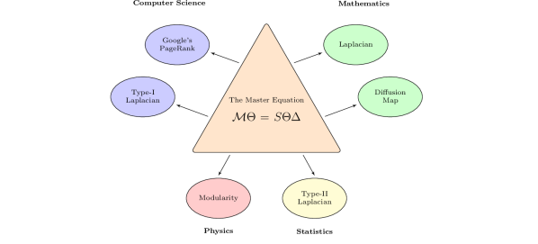
Figure 1: The uniting power of our theory that integrates wide-range of spectral graph methods invented by various researchers from different disciplines.

3 Unified Computing Algorithm

Here we provide the universal construction principle whose significance stems from two considerations: (i) All known spectral graph techniques (shown in Figure 1) are just different manifestations of the following single general algorithm, as shown in Sections 4-5. (ii) What is even more surprising is the fact that this same general recipe can also be used to design faster, more accurate custom-made graph-mining algorithms, as described in Section 6.

Algorithm 1. A Unified Algorithm of Spectral Graph Analysis

 Step 1. Let $\{\xi_{j}(x;\mathcal{G})\}_{1\leq j\leq n}$ to be a discrete orthonormal basis of $\mathscr{L}^{2}(F)$ Hilbert space (The vertex probability measure) satisfying the following conditions:

$$\sum\nolimits_{x}\xi_{j}(x;\mathcal{G})\,\xi_{k}(x;\mathcal{G})\,p(x;\mathcal{G})\,=\,\delta_{jk}.$$

Step 2. $\xi\mapsto\eta$ via quantile transform: Construct $\eta_{j}(u;\mathcal{G}):=\xi_{j}(Q(u;\mathcal{G}))$ on the unit interval $0\leq u\leq 1$.

Step 3. Transform coding of graphs. Construct generalized spectral graph matrix or G-matrix $\mathcal{M}(\xi;\mathcal{G})\in{\mathbb{R}}^{n\times n}$ by:

$$\mathcal{M}[j,k;\xi,\mathcal{G}]\,=\Big{\langle}\eta_{j},\int_{0}^{1}(\mathscr{C}-1)\eta_{k}\Big{\rangle}_{L^{2}[0,1]}=\,\sum_{\ell,m}\xi_{j}(\ell;\mathcal{G})\xi_{k}(m;\mathcal{G})P(\ell,m;\mathcal{G}).$$ (3.1)

$\mathcal{M}(\xi;\mathcal{G})$ can be viewed as a transform coefficient matrix of the orthogonal series expansion of $\mathscr{C}(u,v;\mathcal{G})$ with respect to the product bases $\{\eta_{j}\otimes\eta_{k}\}_{1\leq j,k\leq n}$. Step 4. Perform the singular value decomposition (SVD) of $\mathcal{M}(\xi;\mathcal{G})=U\Lambda U^{T}$ $=\sum_{k}u_{k}\lambda_{k}u_{k}^{T}$, where $u_{ij}$ are the elements of the singular vector of moment matrix $U=(u_{1},\ldots,u_{n})$, and $\Lambda={\rm diag}(\lambda_{1},\ldots,\lambda_{n})$, $\lambda_{1}\geq$ $\cdots\lambda_{n}\geq 0$. Step 5. Obtain approximate Karhunen-Loéve  basis (or simply the graph representation basis) of the graph $\mathcal{G}$ by taking the following linear combination:

$$\widetilde{\phi}_{k}\,=\,\sum_{j=1}^{n}u_{jk}\xi_{j},\,\leavevmode\nobreak\ {\rm for}\,\,k=1,\ldots,n-1,$$

which can be directly used for subsequent signal processing on graphs.  

4 Empirical Spectral Graph Analysis

Three popular traditional spectral graph analysis models will be synthesized in this section as a special case of the master equation (Eq. 2.6 of Theorem 4) and the previous algorithm.

4.1 Laplacian Spectral Analysis

Laplacian is probably the most heavily used spectral graph technique in practice [3, 22, 23, 24, 25]. Here we will demonstrate for the first time how the Laplacian of a graph naturally originates by purely statistical reasoning, totally free from the classical combinatorial based logic.

Degree-Adaptive Block-pulse Basis Functions. One of the fundamental, yet universally valid (for any graph) choice for $\{\eta_{j}\}_{1\leq j\leq n}$ is the indicator top hat functions (also known as block-pulse basis functions, or in short BPFs). However, instead of defining the BPFs on a uniform grid (which is the usual practice) here (following Sec 2.3) we define them on the non-uniform mesh $0=u_{0}<u_{1}\cdots<u_{n}=1$ over [0,1], where $u_{j}=\sum_{x\leq j}p(x;X)$ with local support

$$\eta_{j}(u)=\left\{\begin{array}[]{ll}p^{-1/2}(j)\nobreak\leavevmode\nobreak\leavevmode&\mbox{for $u_{j-1}<u\leq u_{j}$};\\ 0\nobreak\leavevmode\nobreak\leavevmode&\mbox{elsewhere}.\end{array}\right.$$ (4.1)

They are disjoint, orthogonal, and a complete set of functions satisfying

$$\int_{0}^{1}\eta_{j}(u)\;\mathrm{d}u=\sqrt{p(j)},\leavevmode\nobreak\ \leavevmode\nobreak\ \,\int_{0}^{1}\eta_{j}^{2}(u)\;\mathrm{d}u=1,\leavevmode\nobreak\ \leavevmode\nobreak\ \text{and}\leavevmode\nobreak\ \leavevmode\nobreak\ \int_{0}^{1}\eta_{j}(u)\eta_{k}(u)\;\mathrm{d}u=\delta_{jk}.$$

It is interesting to note that the shape (amplitudes and block lengths) of our specially designed BPFs depend on the specific graph structure via $p(x;\mathcal{G})$ as shown in Fig 2. In order to obtain the spectral domain representation of the graph, it is required to estimate the spectra of GraField kernel $\phi_{k}$, by representing them as block pulse series. The next result describes the required computational scheme for estimating the unknown expansion coefficients $\{\theta_{jk}\}$.

Theorem 5.

Let $\phi_{1},\ldots,\phi_{n}$ the canonical Schmidt bases of $\mathscr{L}^{2}$ graph kernel $\mathscr{C}(u,v;\mathcal{G})$, satisfying the integral equation (2.3). Then the empirical solution of (2.3) for block-pulse orthogonal series approximated (4.1) Fourier coefficients $\{\theta_{jk}\}$ can equivalently be written down in closed form as the following matrix eigen-value problem

$$\mathcal{L}^{*}\Theta\,=\,\Theta\Lambda,$$ (4.2)

where $\mathcal{L}^{*}=\mathcal{L}-uu^{T}$, $\mathcal{L}$ is the Laplacian matrix, $u=D_{p}^{1/2}1_{n}$, and $D_{p}={\rm diag}(p_{1},\ldots,p_{n})$.

Proof.

Recall that the discrete GraField kernel ${\rm GIF}(j,k;\mathcal{G})=P(j,k;\mathcal{G})/$ $p(j;\mathcal{G})p(k;\mathcal{G})$ and the tensor product bases $\eta_{j}(u)\otimes\eta_{k}(v)$ take the value $p^{-1/2}(j;\mathcal{G})\times$ $p^{-1/2}(k;\mathcal{G})$ over the rectangle $I_{jk}(u,v)$ for $0<u,v<1$. Substituting this into the master equation (2.9) leads to the following system of linear algebraic equations expressed in the vertex domain:

$$\sum_{j}\theta_{jk}\left[\dfrac{p(j,l)}{\sqrt{p(j)p(l)}}\,-\,\sqrt{p(j)}\sqrt{p(l)}\,-\,\lambda_{l}\delta_{jl}\right]\leavevmode\nobreak\ =\leavevmode\nobreak\ 0.$$ (4.3)

The next step of the proof involves empirical plugin nonparametric estimation as the estimating equation (4.3) contains unknown network and vertex probability mass functions which need to be estimated from the data. The most basic nonparametric estimates are $\widetilde{P}(j,k;\mathcal{G})=A[j,k;\mathcal{G}]/N$ and $\widetilde{p}(j;\mathcal{G})=d(j;\mathcal{G})/N$. By plugging these empirical estimators into Eq. (4.3), said equation can be rewritten as the following compact matrix form:

$$\left[\mathcal{L}-N^{-1}\sqrt{{\bm{d}}}\sqrt{{\bm{d}}}^{T}\right]\tilde{\Theta}=\tilde{\Theta}\tilde{\Lambda},$$ (4.4)

where $\mathcal{L}=D^{-1/2}AD^{-1/2}$ is the graph Laplacian matrix and $\sqrt{{\bm{d}}}=(\sqrt{d_{1}},\ldots,\sqrt{d_{n}})^{T}$. This also leads to an explicit expression for the degree-adaptive BPFs-approximated Karhunen-Loéve  basis $\widetilde{\Phi}=D_{\tilde{p}}^{-1/2}\widetilde{\Theta}$ by combining (2.4) and (4.1). ∎

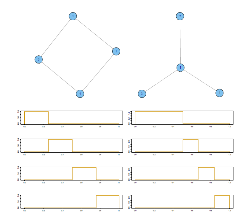
Figure 2: Two graphs and their corresponding degree-adaptive block-pulse functions. The amplitudes and the block length of the indicator basis functions (4.1) depends on the degree distribution of that graph.

Remark 2.

Theorem 5 allows us to interpret the graph Laplacian as the empirical G-matrix $\widetilde{\mathcal{M}}(\eta,\mathcal{G})$ under degree-adaptive indicator basis choice for the $\eta$ shape function. Our technique provides a completely nonparametric statistical derivation of an algorithmic spectral graph analysis tool. The plot of $\widetilde{\lambda}_{k}$ versus $k$ can be considered as a “raw periodogram” analogue for graph data analysis.

4.2 Diffusion Map

We provide a statistical derivation of Coifman’s diffusion map [5] algorithm, which hinges upon the following key result.

Theorem 6.

The empirical GraField admits the following vertex-domain spectral diffusion decomposition at any finite time $t$

$$\dfrac{\widetilde{p}(t,y|x;\mathcal{G})}{\widetilde{p}(y;\mathcal{G})}\leavevmode\nobreak\ =\leavevmode\nobreak\ 1+\sum_{k}\tilde{\lambda}_{k}^{t}\tilde{\phi}_{k}(x)\tilde{\phi}_{k}(y),$$ (4.5)

where $\widetilde{\phi}_{k}=D_{\tilde{p}}^{-1/2}u_{k}$, ($u_{k}$ is the $k$th eigenvector of the Laplacian matrix $\mathcal{L}$), $\widetilde{p}(y|x;\mathcal{G})=\mathcal{T}(x,y)$, $\mathcal{T}=$ $D^{-1}A$ denotes the one-step transition matrix of a random walk on $\mathcal{G}$ with stationary distribution $\tilde{p}(y;\mathcal{G})=d(y;\mathcal{G})/N$ and $p(t,y|x;\mathcal{G})$ is the kernel of the t-th power of $p(y|x;\mathcal{G})$ for $t\geq 0$.

Proof.

We see that from Theorem 5 that the Laplacian approximated GraField  eigen basis is given by $\widetilde{\phi}_{k}=D_{\tilde{p}}^{-1/2}u_{k}$, where $u_{k}$ is the $k$th eigenvector of the Laplacian matrix $\mathcal{L}$. This, together with Theorem 2, immediately imply the following vertex-domain spectral decomposition result of the empirical GraField:

$$\dfrac{\widetilde{p}(y|x;\mathcal{G})}{\widetilde{p}(y;\mathcal{G})}\leavevmode\nobreak\ =\leavevmode\nobreak\ 1+\sum_{k}\tilde{\lambda}_{k}\tilde{\phi}_{k}(x)\tilde{\phi}_{k}(y).$$ (4.6)

This significance of this identity is that it automatically yields the (appropriately normalized) diffusion kernel whose continuous analogue is known as Laplace-Beltrami operator. As $p(y|x;\mathcal{G})$ can be interpreted as the probability of transition in one time step from node $x$ to node $y$, the conclusion is immediate by applying the spectral theory on the $t$-th power of $p(y|x;\mathcal{G})$. For an alternative proof of the expansion (4.6) see Appendix section of Coifman and Lafon (2006) [5] by noting $\widetilde{\phi}_{k}$ are the right eigenvectors of random walk Laplacian $\mathcal{T}$. ∎

Remark 3.

In light of Theorem 6, define diffusion map coordinates at time $t$ as the mapping from $x$ to the vector

$$x\longmapsto\Big{(}\lambda_{1}^{t}\phi_{1}(x),\ldots,\lambda_{k}^{t}\phi_{k}(x)\Big{)},\leavevmode\nobreak\ \leavevmode\nobreak\ \leavevmode\nobreak\ \leavevmode\nobreak\ x\in\{1,2,\ldots,n\},$$

which can be viewed as an approximate ‘optimal’ Karhunen-Loéve  representation basis and thus can be used for non-linear embedding of graphs. Define diffusion distance, a measure of similarity between two nodes of a graph, as the Euclidean distance in the diffusion map space

$$D_{t}^{2}(x,x^{\prime})\leavevmode\nobreak\ =\leavevmode\nobreak\ \sum_{j\geq 1}\lambda_{j}^{2t}\big{\{}\phi_{j}(x)\,-\,\phi_{j}(x^{\prime})\big{\}}^{2}.\leavevmode\nobreak\ \leavevmode\nobreak\ \leavevmode\nobreak\ \leavevmode\nobreak\ \leavevmode\nobreak\ \leavevmode\nobreak\ \leavevmode\nobreak\ \leavevmode\nobreak\ \leavevmode\nobreak\ \leavevmode\nobreak\ \leavevmode\nobreak\$$ (4.7)

This procedure is known as diffusion map, which has been extremely successful tool for manifold learning. Our approach provides an additional insight and justification for the (Laplace-Beltrami) diffusion coordinates by interpreting it as the strength of connectivity profile for each vertex, thus establishing a close connection with empirical GraField.

4.3 Modularity Spectral Analysis

Theorem 7.

To approximate the KL graph basis $\phi_{k}=\sum_{j}\theta_{jk}\eta_{j}$, choose $\eta_{j}(u)=\mathbf{I}(u_{j-1}<u\leq u_{j})$ to be the characteristic function satisfying

$$\int_{0}^{1}\eta_{j}(u)\;\mathrm{d}u\leavevmode\nobreak\ =\leavevmode\nobreak\ \int_{0}^{1}\eta^{2}_{j}(u)\;\mathrm{d}u\leavevmode\nobreak\ =\leavevmode\nobreak\ \,p(j;\mathcal{G}).$$

Then the corresponding empirically estimated spectral graph equation (2.9) can equivalently be reduced to the following generalized eigenvalue equation:

$$\mathcal{B}\Theta\,=\,D\Theta\Lambda,$$ (4.8)

where the matrix $\mathcal{B}$ is given by $A-\frac{1}{{\rm Vol}(\mathcal{G})}{\bm{d}}{\bm{d}}^{T}$, and ${\bm{d}}=A1_{n}$ is the degree vector.

Remark 4.

The matrix $\mathcal{B}$, known as modularity matrix, was introduced by Newman (2006) [4] from an entirely different motivation. Our analysis reveals that the Laplacian and Modularity based spectral graph analyses are equivalent in the sense that they inherently use the same underlying basis expansion (one is a rescaled version of the other) to approximate the optimal graph bases.

Summary of Section 4. Solutions (eigenfunctions) of the GraField estimating equation based on the G-matrix under the proposed specialized nonparametric approximation scheme provides a systematic and unified framework for spectral graph analysis. As an application of this general formulation, we have shown how one can synthesize the well-known Laplacian, diffusion map, and modularity spectral algorithms and view them as “empirical” spectral graph analysis methods. It is one of those rare occasions where one can witness the convergence of statistical, algorithmic and geometry-motivated computational models.

5 Smoothed Spectral Graph Analysis

Smoothness is a universal requirement for constructing credible nonparametric estimators. Spectral graph analysis is also no exception. An improved smooth version of raw-empirical spectral graph techniques will be discussed, revealing a simple and straightforward statistical explanation of the origin of regularized Laplacian techniques. This, as we shall see, also opens up several possibilities for constructing new types of spectral regularization schemes, which seems difficult to guess using previous understanding.

5.1 High-dimensional Undersampled Regime

Recall from Theorem 4 that the generalized matrix eigenvalue equation (2.6) depends on the unknown network and vertex probability mass functions. This leads us to the question of estimating the unknown distribution $P=(p_{1},p_{2},\ldots,p_{n})$ (support size = size of the graph = $n$) based on $N$ sample, where $N=\sum_{i=1}^{n}d_{i}=2|E|$. Previously (Theorems 5-7) we have used the unsmoothed maximum likelihood estimate (MLE) ${\widetilde{p}}(x;\mathcal{G})$ to construct our empirical spectral approximation algorithms, which is the unique minimum variance unbiased estimator. Under standard asymptotic setup, where the dimension of the parameter space $n$ is fixed and the sample size $N$ tends to infinity, the law of large numbers ensures optimality of ${\widetilde{p}}$. As a consequence, empirical spectral analysis techniques are expected to work quite well for dense graphs.

Estimation of probabilities from sparse data. However, the raw ${\widetilde{p}}$ is known to be strictly sub-optimal [26] and unreliable in the high-dimensional sparse-regime where $N/n=O(1)$ (i.e., when parameter dimension and the sample size are comparably large). This situation can easily arise for modern day large sparse graphs where the ratio $N/n$ is small and there are many nodes with low degree, as is the case of degree sparsity. The naive MLE estimator can become unacceptably noisy (high variability) due to the huge size and sparse nature of the distribution. In order to reduce the fluctuations of “spiky” empirical estimates, some form of “smoothing” is necessary. The question remains: How to tackle this high-dimensional discrete probability estimation problem, as this directly impacts the quality of our nonparametric spectral approximation.

Our main purpose in the next section is to describe one such promising technique for smoothing raw-empirical probability estimates, which is flexible and in principle can be applied to any sparse data.

5.2 Spectral Smoothing

We seek a practical solution for circumventing this problem that lends itself to fast computation. The solution, that is both the simplest and remarkably serviceable, is the Laplace/Additive smoothing [27] and its variants, which excel in sparse regimes [28, 26]. The MLE and Laplace estimates of the discrete distribution $p(j;\mathcal{G})$ are respectively given by

$\text{Raw-empirical MLE estimates}:\leavevmode\nobreak\ \leavevmode\nobreak\ \leavevmode\nobreak\ \leavevmode\nobreak\ \leavevmode\nobreak\ \leavevmode\nobreak\ {\widetilde{p}}(j;\mathcal{G})\,=\,\dfrac{d_{j}}{N}\,;\leavevmode\nobreak\ \leavevmode\nobreak\ \leavevmode\nobreak\ \leavevmode\nobreak\ \leavevmode\nobreak\ \leavevmode\nobreak\ \leavevmode\nobreak\ \leavevmode\nobreak\ \leavevmode\nobreak\ \leavevmode\nobreak\ \leavevmode\nobreak\ \leavevmode\nobreak\ \leavevmode\nobreak\ \leavevmode\nobreak\ \leavevmode\nobreak\ \leavevmode\nobreak\ \leavevmode\nobreak\ \leavevmode\nobreak\ \leavevmode\nobreak\ \leavevmode\nobreak\ \leavevmode\nobreak\ \leavevmode\nobreak\ \leavevmode\nobreak\ \leavevmode\nobreak\ \leavevmode\nobreak\ \leavevmode\nobreak\ \leavevmode\nobreak\ \leavevmode\nobreak\ \leavevmode\nobreak\ \leavevmode\nobreak\ \leavevmode\nobreak\ \leavevmode\nobreak\ \leavevmode\nobreak\ \leavevmode\nobreak\ \leavevmode\nobreak\$
$\leavevmode\nobreak\ \leavevmode\nobreak\ \leavevmode\nobreak\ \leavevmode\nobreak\ \leavevmode\nobreak\ \leavevmode\nobreak\ \leavevmode\nobreak\ \leavevmode\nobreak\ \,\text{Smooth Laplace estimates}:\leavevmode\nobreak\ \leavevmode\nobreak\ \leavevmode\nobreak\ \leavevmode\nobreak\ \leavevmode\nobreak\ \leavevmode\nobreak\ \leavevmode\nobreak\ \leavevmode\nobreak\ \leavevmode\nobreak\ \leavevmode\nobreak\ \leavevmode\nobreak\ \leavevmode\nobreak\ \widehat{p}_{\tau}(j;\mathcal{G})\,=\,\dfrac{d_{j}+\tau}{N+n\tau}$         $(j=1,\ldots,n)$. Note that the smoothed distribution $\widehat{p}_{\tau}$ can be expressed as a convex combination of the empirical distribution ${\widetilde{p}}$ and the discrete uniform distribution $1/n$

$$\widehat{p}_{\tau}(j;\mathcal{G})\,=\,\dfrac{N}{N+n\tau}\,\,{\widetilde{p}}(j;\mathcal{G})\,+\,\dfrac{n\tau}{N+n\tau}\,\left(\dfrac{1}{n}\right),\leavevmode\nobreak\ \leavevmode\nobreak\ \leavevmode\nobreak\$$ (5.1)

which provides a Stein-type shrinkage estimator of the unknown probability mass function $p$. The shrinkage significantly reduces the variance, at the expense of slightly increasing the bias.

Choice of $\tau$. The next issue is how to select the “flattening constant” $\tau$. The following choices of $\tau$ are most popular in the literature[28]:

$$\tau=\left\{\begin{array}[]{ll}1&\mbox{Laplace estimator};\\ 1/2&\mbox{Krichevsky\textendash Trofimov estimator};\\ 1/n&\mbox{Perks estimator};\\ \sqrt{N}/n&\mbox{Minimax estimator (under $L^{2}$ loss)}.\end{array}\right.$$

Remark 5.

Under increasing-dimension asymptotics, this class of estimator is often difficult to improve without imposing additional smoothness constraints on the vertex probabilities. The latter may not be a valid assumption as nodes of a graph offer no natural order in general.

With this understanding, smooth generalizations of empirical spectral graph techniques will be discussed, which have a close connection with recently proposed spectral regularized techniques.

5.3 Type-I Regularized Graph Laplacian

Construct $\tau$-regularized smoothed empirical $\eta_{j;\tau}$ basis function by replacing the amplitude $p^{-1/2}(j)$ by $\hat{p}_{\tau}^{-1/2}(j)$ following (5.1). Incorporating this regularized trial basis, we have the following modified G-matrix based linear algebraic estimating equation (2.6):

$$\sum_{j}\theta_{jk}\left[\dfrac{\widetilde{p}(j,k)}{\sqrt{\hat{p}_{\tau}(j)\hat{p}_{\tau}(k)}}\,-\,\sqrt{\hat{p}_{\tau}(j)}\sqrt{\hat{p}_{\tau}(k)}\,-\,\lambda_{k}\delta_{jk}\right]\leavevmode\nobreak\ =\leavevmode\nobreak\ 0.$$ (5.2)

The following theorem follows easily from the preceding calculation.

Theorem 8.

The $\tau$-regularized block-pulse series based spectral approximation scheme is equivalent to representing or embedding discrete graphs in the continuous eigenspace of

$$\text{Type-I Regularized Laplacian}\leavevmode\nobreak\ \leavevmode\nobreak\ =\leavevmode\nobreak\ \leavevmode\nobreak\ D_{\tau}^{-1/2}\,A\,D_{\tau}^{-1/2},\leavevmode\nobreak\ \leavevmode\nobreak\ \leavevmode\nobreak\ \leavevmode\nobreak\ \leavevmode\nobreak\ \leavevmode\nobreak\ \leavevmode\nobreak\ \leavevmode\nobreak\ \leavevmode\nobreak\ \leavevmode\nobreak\ \leavevmode\nobreak\ \leavevmode\nobreak\$$ (5.3)

where $D_{\tau}$ is a diagonal matrix with $i$-th entry $d_{i}+\tau$.

Remark 6.

It is interesting to note that this exact regularized Laplacian formula was proposed by Chaudhuri et al. (2012) [6] as well as Qin and Rohe (2013) [29], albeit from a very different motivation.

5.4 Type-II Regularized Graph Laplacian

Theorem 9.

Estimate the joint probability $p(j,k;\mathcal{G})$ by extending the formula given in (5.1) for the two-dimensional case as follows:

$$\widehat{p}_{\tau}(j,k;\mathcal{G})\,\,=\,\,\dfrac{N}{N+n\tau}\,\,{\widetilde{p}}(j,k;\mathcal{G})\,+\,\dfrac{n\tau}{N+n\tau}\,\left(\dfrac{1}{n^{2}}\right),\leavevmode\nobreak\ \leavevmode\nobreak\ \leavevmode\nobreak\ \leavevmode\nobreak\ \leavevmode\nobreak\ \leavevmode\nobreak\$$ (5.4)

which is equivalent to replacing the original adjacency matrix by $A_{\tau}=A+(\tau/n){\bf 1}{\bf 1}^{T}$. This modification via smoothing in the estimating equation (5.2) leads to the following spectral graph matrix

$$\text{Type-II Regularized Laplacian}\leavevmode\nobreak\ \leavevmode\nobreak\ =\leavevmode\nobreak\ \leavevmode\nobreak\ D_{\tau}^{-1/2}\,A_{\tau}\,D_{\tau}^{-1/2}.\leavevmode\nobreak\ \leavevmode\nobreak\ \leavevmode\nobreak\ \leavevmode\nobreak\ \leavevmode\nobreak\ \leavevmode\nobreak\ \leavevmode\nobreak\ \leavevmode\nobreak\ \leavevmode\nobreak\ \leavevmode\nobreak\ \leavevmode\nobreak\ \leavevmode\nobreak\$$ (5.5)

Remark 7.

Exactly the same form of regularization of Laplacian graph matrix (5.5) was proposed by Amini et al. (2013) [7] as a fine-tuned empirical solution.

5.5 Google’s PageRank Method

Smoothing of network and vertex probability distributions appearing in generalized matrix equation (2.6) resulted in Type-I and Type-II regularized Laplacian methods. The third possibility is to directly smooth the conditional or transitional probability matrix to develop a regularized version of random walk Laplacian (which we call Type-III regularized Laplacian) method for large sparse graphs. Smoothing conditional probability function. Consider a random walk on $\mathcal{G}$ with transition probability $\mathcal{T}(i,j;\mathcal{G})=\Pr(X_{t+1}=j|X_{t}=i)\geq 0$. Note that the smoothing (5.4) can equivalently be represented as

$$\widehat{\mathcal{T}}_{\tau}(i,j;\mathcal{G})\,\,=\,\,\dfrac{A(i,j;\mathcal{G})+\tau/n}{d_{i}+\tau}\,\,=\,\,(1-\alpha_{\tau})\widetilde{\mathcal{T}}(i,j;\mathcal{G})\,+\,\alpha_{\tau}\left(\dfrac{1}{n}\right),$$ (5.6)

where the degree-adaptive regularization parameter $\alpha_{\tau}=\tau(d_{i}+\tau)^{-1}$ and empirical transition matrix $\widetilde{\mathcal{T}}=D^{-1}A$.

Theorem 10.

Smooth each row of empirical random walk Laplacian $\widetilde{\mathcal{T}}$ (as it is a row-stochastic or row-Markov matrix) via Stein-like shrinkage to construct an equivalent and more simplified (non-adaptive) estimator:

$$\text{Type-III Regularized Laplacian}\leavevmode\nobreak\ \leavevmode\nobreak\ =\leavevmode\nobreak\ \leavevmode\nobreak\ (1-\alpha)\widetilde{\mathcal{T}}\,+\,\alpha F,\leavevmode\nobreak\ \leavevmode\nobreak\ \leavevmode\nobreak\ \leavevmode\nobreak\ 0<\alpha<1,$$ (5.7)

where $F$ is a rank-one matrix given by $\frac{1}{n}{\bf 1}{\bf 1}^{T}$.

Remark 8.

The non-adaptive regularized random-walk Laplacian matrix $\mathcal{T}_{\alpha}$ (5.7) was introduced by Larry Page and Sergey Brin in 1996 [8] and is called the Google’s PageRank matrix. What seems natural enough from our nonparametric smoothing perspective, is in fact known to be highly surprising adjustment–the “Teleportation trick”.

‘Teleporting is the essential distinguishing feature of the PageRank random walk that had not appeared in the literature before’ – Vigna (2005)[30].

Remark 9.

The Google’s PageRank matrix (which is different from the empirical random walk Laplacian in an important way) is probably the most famous, earliest, and spectacular example of spectral regularization that was originally introduced to counter the problem of dangling nodes (nodes with no outgoing edges) by “connecting” the graph. As a result the random walk can teleport to a web page uniformly at random (or adaptively based on degree-weights) whenever it hits a dead end. The steady state vector describes the long term visit rate–the PageRank score, computed via eigen-decomposition of $\mathcal{T}_{\alpha}$.

5.6 Other Generalizations

The beauty of our statistical argument is that it immediately opens up several possibilities to construct new types of spectral regularization schemes, which are otherwise hard to guess using previous understanding. Two such promising techniques are discussed here. The first one deals with Stein smoothing with data-driven shrinkage parameter. We refine the smooth nonparametric spectral graph models (discussed in previous Sections 5.2-5.5) by wisely choosing the regularization parameter $\tau$: from fixed $\tau$ to data-driven $\widehat{\tau}$. Quite surprisingly, the explicit formula of the empirical optimal $\widehat{\tau}^{*}$ can be derived by minimizing the squared error loss risk function, as given in the following theorem.

Theorem 11.

Under the mean square error (MSE) risk function, the Stein-optimal shrinkage parameter and its consistent estimator is given by

$$\widehat{\tau}^{*}\leavevmode\nobreak\ =\leavevmode\nobreak\ \dfrac{N^{2}-\sum_{i=1}^{n}d_{i}^{2}}{n\sum_{i=1}^{n}d_{i}^{2}-N^{2}}.$$ (5.8)

Proof.

Our theory of determining optimal shrinkage parameter starts by explicitly writing down the risk function:

$${\rm MSE}(\widehat{p}_{\tau},p)\,:=\,R(\tau)\,=\,\sum_{i=1}^{n}\mathbb{E}\big{(}\widehat{p}_{\tau}(i;\mathcal{G})-p(i;\mathcal{G})\big{)}^{2},$$

Replacing by $\widehat{p}_{\tau}(i;\mathcal{G})$ by (5.1), after some routine calculations, we get

$$R(\tau)\,=\,\Big{(}1-\dfrac{2n\tau}{N+n\tau}\Big{)}{\rm Var}({\widetilde{p}}(i;\mathcal{G}))\,+\,\Big{(}\dfrac{n\tau}{N+n\tau}\Big{)}^{2}\mathbb{E}\big{(}{\widetilde{p}}(i;\mathcal{G})-1/n\big{)}^{2},$$ (5.9)

Analytically minimizing the total risk function (5.9) with respect to $\tau$ by setting $R^{\prime}(\tau)$ = 0, leads to the following optimal choice:

$$\tau^{*}\,=\,\frac{N}{n}\times\dfrac{\sum_{i=1}^{n}{\rm Var}({\widetilde{p}}(i;\mathcal{G}))}{\sum_{i=1}^{n}\big{[}\mathbb{E}({\widetilde{p}}(i;\mathcal{G})-1/n)^{2}-{\rm Var}({\widetilde{p}}(i;\mathcal{G}))\big{]}}.$$ (5.10)

As variance of the MLE estimate ${\rm Var}({\widetilde{p}}(i;\mathcal{G}))=p(i;\mathcal{G})(1-p(i;\mathcal{G}))/N$, we can further simplify the formula (5.10) as

$$\tau^{*}\,=\,\dfrac{1-\sum_{i=1}^{n}p^{2}(i;\mathcal{G})}{n\sum_{i=1}^{n}p^{2}(i;\mathcal{G})-1}.$$

The proof follows by replacing the unknown network probabilities by their empirical counterparts ${\widetilde{p}}(i;\mathcal{G})=d_{i}/N$. ∎

Remark 10.

The significance of this result lies in the fact that the optimal regularization parameter $\tau$ can be determined with no additional computation in a completely data-driven fashion. The formula (5.8) provides an analytic expression that guarantees to minimize the MSE avoiding the need of computationally expensive cross-validation like methods. It is shown in Supplementary Appendix D that proposed method performs 100x faster and uses 1000x less memory for moderately large problems than the current best practice.

While the Laplace or additive smoothing performs well in general, there are situations where they perform poorly [31]. The Good-Turing estimator [32] is often the next best choice which is given by

$$\widehat{p}_{{\rm GT}}(i;\mathcal{G})\leavevmode\nobreak\ =\leavevmode\nobreak\ \dfrac{\varpi_{d_{i}+1}}{\varpi_{d_{i}}}\cdot\dfrac{d_{i}+1}{N},$$ (5.11)

where $\varpi_{d_{k}}$ denotes the number of nodes with degree $k$. An excellent discussion on this topic can be found in Orlitsky et al. (2003) [33]. One can plug in the estimate (5.11) into the equation (5.2) to generate new spectral graph regularization technique. Summary of Section 5. We wish to emphasize that our novelty lies in addressing the open problem of obtaining a rigorous interpretation and extension of spectral regularization. To the best of our knowledge this is the first work that provides a more formal and intuitive understanding of the foundation of spectral regularization. We have shown how the regularization naturally arises as a consequence of high-dimensional discrete data smoothing.

6 Going Beyond: An Enhanced Method for Accelerated Graph-Learning

Traditional spectral graph analysis techniques do not scale gracefully with the size of the graph, which caused a major practical obstacle to applying them for large-scale problems. As the size of the datasets is growing rapidly, the key challenge is to find an improved representation of graphs that allows compression. In the following, we demonstrate through examples, how our general theory can be used to find such custom-designed compressors for fast and efficient spectral graph analysis.

6.1 Motivating Example and Challenges

We consider the voting records of the US Senate covering the period from the inauguration of George H. W. Bush in January 1989 to the end of Bill Clinton’s term in January 2001 (retrieved from www.voteview.com). Table 1 portrays a snapshot of the dataset, where $n=2678$ bills were submitted over the period and binary voting decisions ($1$ for yes, $0$ for no) were recorded from each of the $100$ seats.

Table 1: Data corresponding to the voting record of the US Senate covering the period from Jan 1989 to Jan 2001. Source: www.voteview.com.

Time	Bills	Senate Seats
		1	2	3	$\cdots$	98	99	100
1989-02-28	1	0	1	1	$\cdots$	1	0	1
1989-02-28	2	0	1	0	$\cdots$	1	0	0
$\vdots$		$\vdots$		$\vdots$		$\vdots$		$\vdots$
2000-12-05	2677	1	1	1	$\cdots$	0	1	1
2000-12-07	2678	1	1	1	$\cdots$	0	1	1

Previously[34, 35] this dataset was analyzed for studying changes in voting patterns to better understand the political polarization among Republican and Democratic senators in the U.S. Congress. Broadly speaking, this problem falls under the category of high-dimensional change-point detection, a critical task in many fields, including econometrics, signal processing, climatology, genomics, neuroscience, speech recognition, and medical monitoring. We observe an ordered sequence of $d$-dimensional data ${\bf Z}_{t}=(Z_{t1},Z_{t2},\ldots,Z_{td})^{\prime}$ for $t=1,\ldots,n$ and the interest lies in tracking $\{{\bf Z}_{t};t=1,\ldots,n\}$ for possible distributional shift:

$$\hskip 108.405pt{\bf Z}_{t}=\left\{\begin{array}[]{ll}F_{1}&\mbox{if $1\leq t\leq\tau_{1}$}\\ F_{2}&\mbox{if $\tau_{1}<t\leq\tau_{2}$}\\ \vdots&\leavevmode\nobreak\ \leavevmode\nobreak\ \leavevmode\nobreak\ \leavevmode\nobreak\ \vdots\\ F_{k}&\mbox{if $\tau_{k}<t\leq\tau_{k+1}=n$},\end{array}\right.$$

where the locations ($\tau_{i};i=1,\ldots,k$), the number of change points $k$, and the distributions $F_{i},$ $i=1,\ldots,k$ in $\mathbb{R}^{d}$ are all unknown. The goal is simple: to develop a fully nonparametric algorithm for automatic detection of multiple change-points. One way to attack this problem is to transform it into a graph problem. For the Senate data, we construct a network of size $n$ with vertices as the time points (or, equivalently, the bills), and the level of agreement between two voting records was calculated using the Pearson-$\phi^{2}$ coefficient, a measure of association for two binary variables. This time-indexed graph, which we call $\mathbb{T}$-graph, encodes the temporal dynamics of the high-dimensional data. In particular, the problem of finding the change-points (splitting the data into different homogeneous time segments) can now be viewed as a spectral clustering exercise on the $\mathbb{T}$-graph. For more discussion on spectral clustering see Supplementary Appendix B.

As we attempt to partition the network based on $\widetilde{\phi}_{1}$, the leading singular vector of the Laplacian matrix as depicted in Fig. 3, we almost immediately hit a wall. The challenge comes from two principal directions: statistical and computational. The general-purpose Laplacian yields an extremely noisy embedding (the blue dots in Fig. 3). As a result, the spectral clustering completely fails to segment the time periods into homogeneous blocks to identify the ‘smooth’ transition of the voting patterns around Jan, 1995. The problem is further aggravated by the fact that the classical spectral-partitioning methods are prohibitively expensive, with an $O(n^{2})$ cost. In particular, explicitly computing the SVD of the $n\times n$ Laplacian matrix may not be practical or even feasible for massive-scale problems. Rather than implementing off-the-shelf existing methods in a brute-force manner, one may wonder whether there exists any elegant approach for smoothed and accelerated spectral graph learning. What if we could take advantage of the ‘internal structure’ of the problem? Note that our $\mathbb{T}$-graph is endowed with a special structure, not an arbitrary one. The nodes have some kind of natural ordering, which introduces a smoothly varying shape in the Laplacian singular vector, as is clearly visible in Fig. 3. Once we recognize this, the following question becomes obvious: how to build an efficient and robust computational algorithm that can leverage the special structure of the $\mathbb{T}$-graph? This is where our new statistical point of view comes in handy .

6.2 Compressive Trial-Basis Design

The key is to intelligently design the trial-basis functions that take into account the additional structure of the problem. In particular, $\{\phi_{k}\}$ must be compressible in the new basis, i.e., we need fewer terms (say, $m$, where $m\ll n)$ in the expansion (2.4) to achieve the target accuracy. One such discrete-orthonormal system (called LP-graph basis) is given below, inspired by the recent work of Mukhopadhyay, Parzen, and their colleague[36, 37, 38].

To set the stage, we start with a brief overview of the manufacturing process for an arbitrary discrete random variable $X$ with pmf $p(x;X)$ and cdf $F(x;X)$. Construct the basis functions of $X$ by Gram Schmidt orthonormalization of powers of $T_{1}(x;X)$, given by

$$T_{1}(x;X)\,=\,\dfrac{\sqrt{12}[F^{\rm{mid}}(x;X)-.5]}{\sqrt{1-\sum_{x}p^{3}(x;X)}},$$ (6.1)

where $F^{\rm{mid}}(x;X)=F(x;X)-.5p(x;X)$ denotes the mid-distribution function. It is easy to verify that these basis functions satisfy the desired orthonormality conditions (see Sec 2.3):

$$\sum_{i}T_{j}(x_{i};X)p(x_{i};X)=0,\sum_{i}T^{2}_{j}(x_{i};X)p(x_{i};X)=1,\sum_{i}T_{j}(x_{i};X)T_{k}(x_{i};X)p(x_{i};X)=0.$$ (6.2)

We define LP orthonormal basis in the unit interval (rescaling operation) by evaluating $T_{j}$ at $Q(u;X)$, quantile function of the random variable $X$

$$S_{j}(u;X)\,=\,T_{j}(Q(u;X);X),\leavevmode\nobreak\ \leavevmode\nobreak\ 0<u<1.$$ (6.3)

For undirected weighted graph $\mathcal{G}$, construct the data-adaptive basis $\{S_{j}(u;\mathcal{G})\}$ by choosing the discrete distribution to be the empirical vertex probability mass function ${\widetilde{p}}(x;\mathcal{G})=\sum_{y=1}^{n}A(x,y;\mathcal{G})/{\rm Vol}(\mathcal{G})$, where ${\rm Vol}(\mathcal{G})=\sum_{x,y}A(x,y;\mathcal{G})$. The Eq (6.2) guarantees that the orthonormal system is automatically degree-weighted. One notable aspect of the LP-graph basis is its nonparametric nature (not fixed like discrete Fourier basis, wavelets, or curvelets, etc.), in the sense that its shape depends on the given graph structure.

6.3 LP-Frequency Domain Analysis

To prepare for the main result, here we introduce a Fourier-like transform, called LP-transform coding of graphs, define by

$$\operatorname{LP}[j,k;\mathcal{G}]\,\leavevmode\nobreak\ \leavevmode\nobreak\ =\,\leavevmode\nobreak\ \leavevmode\nobreak\ \big{\langle}T_{j},T_{k}\big{\rangle}_{L^{2}({\widetilde{p}})}\,\leavevmode\nobreak\ \leavevmode\nobreak\ =\,\leavevmode\nobreak\ \leavevmode\nobreak\ \big{\langle}S_{j},\int_{0}^{1}\mathscr{C}\,S_{k}\big{\rangle}_{L^{2}[0,1]}\leavevmode\nobreak\ \leavevmode\nobreak\ \leavevmode\nobreak\ \leavevmode\nobreak\ (j,k=1,\ldots,m).$$ (6.4)

This is in fact the G-matrix with respect to an LP-orthonormal system (3.1). As a practical significance, this provides a systematic recipe for converting the graph problem into a “suitable” data-driven reduced dimensional ($m\ll n$) matrix problem:

$$\leavevmode\nobreak\ \leavevmode\nobreak\ \leavevmode\nobreak\ \mathcal{G}(V,E)\leavevmode\nobreak\ \leavevmode\nobreak\ \leavevmode\nobreak\ \longrightarrow\leavevmode\nobreak\ \leavevmode\nobreak\ \leavevmode\nobreak\ A_{n\times n}\leavevmode\nobreak\ \leavevmode\nobreak\ \leavevmode\nobreak\ \leavevmode\nobreak\ \longrightarrow\leavevmode\nobreak\ \leavevmode\nobreak\ \leavevmode\nobreak\ \leavevmode\nobreak\ \mathscr{C}(u,v;\mathcal{G})\leavevmode\nobreak\ \leavevmode\nobreak\ \leavevmode\nobreak\ \leavevmode\nobreak\ \xrightarrow[\,\,{\rm Eq.}\,(\ref{eq:LPT})]{\{S_{1},\ldots,S_{m}\}}\leavevmode\nobreak\ \leavevmode\nobreak\ \leavevmode\nobreak\ \leavevmode\nobreak\ \operatorname{LP}\,\in\,{\mathbb{R}}^{m\times m}.\leavevmode\nobreak\ \leavevmode\nobreak\ \leavevmode\nobreak\ \leavevmode\nobreak\ \leavevmode\nobreak\ \leavevmode\nobreak\$$

The purpose of the next result is to describe how to obtain smooth $\widehat{\phi}_{k}$ by performing SVD on the smaller-dimensional $\operatorname{LP}_{m\times m}$ matrix instead of operating on the $n\times n$ dimensional Laplacian matrix, thereby significantly accelerating the computation. In other words, how to estimate the unknown coefficients of (2.4) when we approximate $\phi_{k}(u)$ by $\sum_{j=1}^{m}\theta_{jk}S_{j}(u)$? The following theorem allows us to pin down the formula.

Theorem 12.

Let $\phi_{1},\ldots,\phi_{k_{0}}$ be the top $k_{0}$ canonical Schmidt bases of $\mathscr{L}^{2}$ graph kernel $\mathscr{C}(u,v;\mathcal{G})$, satisfying the integral equation (2.3). Then the empirical solution of (2.3) for LP-orthogonal series approximated (6.3) Fourier coefficients $\{\theta_{jk}\}$ can equivalently be written down in closed form as the following matrix eigen-value problem:

$$\hskip 144.54pt\operatorname{LP}\Theta\,=\,\Theta\Sigma,$$ (6.5)

which leads to the smooth estimate $\widehat{\Phi}=SU_{\operatorname{LP}}$, where $\Phi=[\phi_{1},\ldots,\phi_{k_{0}}]$, $S=[S_{1},\ldots,S_{m}]$, and $U_{\operatorname{LP}}\in{\mathbb{R}}^{m\times m}$ are the matrix of singular vectors of $\operatorname{LP}$ with singular values $\sigma_{1}\geq$ $\cdots\sigma_{m}\geq 0$ and $\Sigma={\rm diag}(\sigma_{1},\ldots,\sigma_{m})$.

Consequently, we represent the graph in the “LP-space,” since important structural information can be compressed into fewer discrete LP-transform coefficients. As an immediate result, we obtain the following reduced-order spectral algorithm.

Algorithm 2: LP-Nonparametric Spectral Learning of $\mathbb{T}$-Graph

 Step 1. Inputs: $A$: the weighted adjacency matrix; $m$: LP-smoothing parameter; $k_{0}$: the desired number of top singular vectors to be approximated. Step 2. Construct the piecewise-constant orthonormal LP-graph polynomial basis $\{S_{1}(u;\mathcal{G}),$ $\ldots,S_{m}(u;\mathcal{G})\}$ using the recipe of Section 6.2: Step 3. Compute $m\times m$ LP-graph transform matrix by the empirical estimate of (6.4):

$$\operatorname{LP}[j,k;\mathcal{G}]\,=\,\mathop{\sum\sum}_{x,y\in V(\mathcal{G})}{\widetilde{p}}(x,y;\mathcal{G})\,S_{j}[\widetilde{F}(x;\mathcal{G})]\,S_{k}[\widetilde{F}(y;\mathcal{G})],\leavevmode\nobreak\ \leavevmode\nobreak\ \leavevmode\nobreak\ 1\leq j,k\leq m.$$

Step 4. Perform the singular value decomposition (SVD) of $\operatorname{LP}=U_{\operatorname{LP}}\Lambda U_{\operatorname{LP}}^{T}=\sum_{k}u_{k}\sigma_{k}u_{k}^{T}$, where $u_{ij}$ are the elements of the singular vector of moment matrix $U_{\operatorname{LP}}=(u_{1},\ldots,u_{m})$, and $\Lambda={\rm diag}(\sigma_{1},\ldots,\sigma_{m})$, $\sigma_{1}\geq$ $\cdots\sigma_{m}\geq 0$. Step 5. Obtain the LP-smoothed graph-Fourier basis by

$$\widehat{\phi}_{k}\,=\,\sum_{j=1}^{m}u_{jk}S_{j},\,\leavevmode\nobreak\ {\rm for}\,\,k=1,\ldots,k_{0}.$$

These “generalized graph-coordinates” can now be used directly for subsequent learning.  

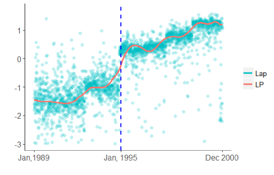
Figure 3: Spectral plot for Senate data. The ‘spiky’ blue dots denote the Laplacian eigenmap, and the ‘smooth’ red line is the LP-approximated graph-Fourier basis. The dashed blue line indicates the estimated change point (Jan 19, 1995), which is almost indistinguishable from the true change point Jan 17, 1995, when the partisan polarization reached a historically high level.

6.4 US Senate Data Analysis

Our LP-nonparametric spectral approximation algorithm yields the ‘smooth’ red curve in Fig 3. Contrast this with the noisy Laplacian singular embedding. Applying k-means clustering on the estimated $\widehat{\phi}_{1}$ (see Supp Fig. 9 for more details) produces two groups with the change point at January 19th, 1995 (1235th record). This comes close to January 17th, 1995 at the beginning of the tenure of the 104th Congress, when Republicans took control the US House of Representatives for the first time since 1956. According to Moody and Mucha (2013)[34], this time period witnessed historically high level of partisan polarization not seen in nearly 100 years.

The specially-designed LP-basis functions require only $m$ coefficients (here we have used $m=15$) instead of $n$ to approximate the Karhunen-Loéve  graph-basis and achieve a remarkable compression ratio of $2678/15=178.53$. This reduces the memory footprint and speeds up the computation. For the Senate data, LP delivers 350x speedup compared to the Laplacian-based traditional method!

Summary of Section 6. Three unique benefits of our nonparametric spectral algorithm are: compressibility, smoothness, and structure-awareness. Additional simulation results are reported in Supplementary Appendix E to highlight the robustness and computational efficiency of the proposed scheme.

7 Concluding Remarks

Our research takes aim at some foundational questions about complex network modeling that are still unsolved. The prescribed approach brings a fresh statistical perspective to accomplish the miracle of unifying and generalizing the existing paradigm, leading to fundamentally new theoretical and algorithmic developments. It was a great surprise for us to be able to deduce existing techniques (which are often viewed as spectral heuristic-based empirical mystery facts) from some underlying basic principles in a self-consistent way. However, from a practical standpoint, we have shown how this new way of thinking about graphs can provide the adequate guidance for designing next-generation computational tools for large-scale problems. It is our hope that a comprehensive understanding gained from this new perspective will provide useful insights for analyzing a wealth of new phenomena that arise in modern network science [39, 40, 41, 42].

Author contributions statement

S.M. conceived the research and wrote the paper. K.W. managed the data collection. S.M. and K.W. conducted the analyses, building the models, and prepared the figures. All authors reviewed the manuscript.

Additional information

Supplementary information: Available online along with all datasets used in the paper. It contains five real data applications, simulation results, further details on the methods and mathematical proofs. Competing Interests: The authors declare no competing interests.

References

- [1] Spielman, D. A. Spectral graph theory and its applications. In 48th Annual IEEE Symposium on Foundations of Computer Science, 29–38 (2007).
- [2] Von Luxburg, U. A tutorial on spectral clustering. \JournalTitleStatistics and computing 17, 395–416 (2007).
- [3] Chung, F. R. Spectral graph theory, vol. 92 (American Mathematical Soc., 1997).
- [4] Newman, M. E. Finding community structure in networks using the eigenvectors of matrices. \JournalTitlePhysical review E 74, 036104 (2006).
- [5] Coifman, R. R. & Lafon, S. Diffusion maps. \JournalTitleApplied and computational harmonic analysis 21, 5–30 (2006).
- [6] Chaudhuri, K., Graham, F. C. & Tsiatas, A. Spectral clustering of graphs with general degrees in the extended planted partition model. \JournalTitleJournal of Machine Learning Research Workshop and Conference Proceedings 35, 1–23 (2012).
- [7] Amini, A. A., Chen, A., Bickel, P. J. & Levina, E. Pseudo-likelihood methods for community detection in large sparse networks. \JournalTitleThe Annals of Statistics 41, 2097–2122 (2013).
- [8] Brin, S. & Page, L. The anatomy of a large-scale hypertextual web search engine. \JournalTitleComputer networks 56, 3825–3833 (1999).
- [9] Fiedler, M. Algebraic connectivity of graphs. \JournalTitleCzechoslovak Mathematical Journal 23, 298–305 (1973).
- [10] Blackman, R. B. & Tukey, J. W. The measurement of power spectra from the point of view of communications engineering (New York, Dover, 1958).
- [11] Tukey, J. W. Data analysis and the frontiers of geophysics: More can be learned from data by wise use of spectrum analysis, choice of expression, and straggling values. \JournalTitleScience 148, 1283–1289 (1965).
- [12] Parzen, E. The role of spectral analysis in time series analysis. \JournalTitleReview of the International Statistical Institute 125–141 (1967).
- [13] Wiener, N. Generalized harmonic analysis. \JournalTitleActa mathematica 55, 117–258 (1930).
- [14] Lovász, L. Random walks on graphs. \JournalTitleCombinatorics, Paul erdos is eighty 2, 1–46 (1993).
- [15] Zachary, W. W. An information flow model for conflict and fission in small groups. \JournalTitleJournal of anthropological research 33, 452–473 (1977).
- [16] Lovász, L. & Szegedy, B. Limits of dense graph sequences. \JournalTitleJournal of Combinatorial Theory, Series B 96, 933–957 (2006).
- [17] Hoeffding, W. Massstabinvariante korrelationstheorie. \JournalTitleSchriften des Mathematischen Seminars und des Instituts fur Angewandte Mathematik der Universitat Berlin 5, 179–233. (1940).
- [18] Schmidt, E. Zur Theorie der linearen und nicht linearen Integralgleichungen Zweite Abhandlung. \JournalTitleMathematische Annalen 64, 433–476 (1907).
- [19] Loève, M. Probability Theory; Foundations, Random Sequences (New York: D. Van Nostrand Company, 1955).
- [20] Parzen, E. Nonparametric statistical data modeling (with discussion). \JournalTitleJournal of the American Statistical Association 74, 105–131 (1979).
- [21] Galerkin, B. Series development for some cases of equilibrium of plates and beams (in Russian). \JournalTitleWjestnik Ingenerow Petrograd 19, 897–908 (1915).
- [22] Tenenbaum, J. B., De Silva, V. & Langford, J. C. A global geometric framework for nonlinear dimensionality reduction. \JournalTitlescience 290, 2319–2323 (2000).
- [23] Shi, J. & Malik, J. Normalized cuts and image segmentation. \JournalTitleIEEE Transactions on Pattern analysis and Machine intelligence 22, 888–905 (2000).
- [24] Belkin, M. & Niyogi, P. Laplacian eigenmaps and spectral techniques for embedding and clustering. \JournalTitleNIPS 14, 585–591 (2001).
- [25] Christiano, P., Kelner, J. A., Madry, A., Spielman, D. A. & Teng, S.-H. Electrical flows, laplacian systems, and faster approximation of maximum flow in undirected graphs. In Proceedings of the forty-third annual ACM symposium on Theory of computing, 273–282 (ACM, 2011).
- [26] Witten, I. H. & Bell, T. The zero-frequency problem: estimating the probabilities of novel events in adaptive text compression. \JournalTitleInformation Theory, IEEE Transactions on 37, 1085–1094 (1991).
- [27] Laplace, P. S. A philosophical essay on probabilities, translated from the 6th French edition by Frederick Wilson Truscott and Frederick Lincoln Emory (Dover Publications, New York, 1951).
- [28] Fienberg, S. E. & Holland, P. W. Simultaneous estimation of multinomial cell probabilities. \JournalTitleJournal of the American Statistical Association 68, 683–691 (1973).
- [29] Qin, T. & Rohe, K. Regularized spectral clustering under the degree-corrected stochastic blockmodel. In Advances in Neural Information Processing Systems, 3120–3128 (2013).
- [30] Vigna, S. Trurank: taking pagerank to the limit. \JournalTitle14th international conference on World Wide Web 976–977 (2005).
- [31] Gale, W. & Church, K. What is wrong with adding one. \JournalTitleCorpus-based research into language 1, 189–198 (1994).
- [32] Good, I. J. The population frequencies of species and the estimation of population parameters. \JournalTitleBiometrika 40, 237–264 (1953).
- [33] Orlitsky, A., Santhanam, N. P. & Zhang, J. Always good turing: Asymptotically optimal probability estimation. \JournalTitleScience 302, 427–431 (2003).
- [34] Moody, J. & Mucha, P. J. Portrait of political party polarization. \JournalTitleNetwork Science 1, 119–121 (2013).
- [35] Roy, S., Atchadé, Y. & Michailidis, G. Change point estimation in high dimensional markov random-field models. \JournalTitleJournal of the Royal Statistical Society: Series B 79, 1187–1206 (2017).
- [36] Mukhopadhyay, S. & Parzen, E. Nonlinear time series modeling: A unified perspective, algorithm, and application. \JournalTitleJournal of Risk and Financial Management: Special Issue on “Applied Econometrics”. 8, 1–18 (2018).
- [37] Mukhopadhyay, S. & Parzen, E. LP approach to statistical modeling. \JournalTitlearXiv:1405.2601 (2014).
- [38] Mukhopadhyay, S. & Fletcher, D. Generalized empirical Bayes modeling via frequentist goodness-of-fit. \JournalTitleNature Scientific Reports 8 (9983), 1–15 (2018).
- [39] Wang, H. & Marron, J. Object oriented data analysis: Sets of trees. \JournalTitleThe Annals of Statistics 1849–1873 (2007).
- [40] Lazer, D. et al. Life in the network: the coming age of computational social science. \JournalTitleScience 323, 721 (2009).
- [41] Kolaczyk, E. D. Topics at the Frontier of Statistics and Network Analysis:(re) visiting the Foundations (Cambridge University Press, 2017).
- [42] Wasserman, L. Topological data analysis. \JournalTitleAnnual Review of Statistics and Its Application (2016).
Acknowledgements
The first author benefited greatly from many fruitful discussions and exchanges of ideas he had at the John W. Tukey 100th Birthday Celebration meeting, Princeton University September 18, 2015. This research was also presented at the Parzen Memorial Lecture, 2017 Joint Statistical Meetings–Baltimore, Maryland. We dedicate this research to the beloved memory of Emanuel (Manny) Parzen, 1929–2016.