A Scale-Separated Approach for Studying Coupled Ion and Electron Scale Turbulence

Abstract

Multiple space and time scales arise in plasma turbulence in magnetic confinement fusion devices because of the smallness of the square root of the electron-to-ion mass ratio $\left(m_{\rm{e}}/m_{\rm{i}}\right)^{1/2}$ and the consequent disparity of the ion and electron thermal gyroradii and thermal speeds. Direct simulations of this turbulence that include both ion and electron space-time scales indicate that there can be significant interactions between the two scales. The extreme computational expense and complexity of these direct simulations motivates the desire for reduced treatment. By exploiting the scale separation between ion and electron scales, and expanding the gyrokinetic equations for the turbulence in $\left(m_{\rm{e}}/m_{\rm{i}}\right)^{1/2}$, we derive such a reduced system of gyrokinetic equations that describes cross-scale interactions. The coupled gyrokinetic equations contain novel terms which provide candidate mechanisms for the observed cross-scale interaction. The electron scale turbulence experiences a modified drive due to gradients in the ion scale distribution function, and is advected by the ion scale $E\times B$ drift, which varies in the direction parallel to the magnetic field line. The largest possible cross-scale term in the ion scale equations is sub-dominant in our $\left(m_{\rm{e}}/m_{\rm{i}}\right)^{1/2}$ expansion. Hence, in our model the ion scale turbulence evolves independently of the electron scale turbulence. To complete the scale-separated approach, we provide and justify a parallel boundary condition for the coupled gyrokinetic equations in axisymmetric equilibria based on the standard “twist-and-shift” boundary condition. This approach allows one to simulate multi-scale turbulence using electron scale flux tubes nested within an ion scale flux tube.

Keywords: Gyrokinetics, Turbulence, Multi-Scale, Cross-Scale Interaction, Transport, Magnetic Confinement Fusion

Prepared for submission to: Plasma Phys. Control. Fusion

1 Introduction

Anomalous transport of heat and particles is a major limiting factor in the performance of tokamaks. The dominant transport mechanism is turbulence arising from micro-instabilities that are driven by macroscopic gradients of the plasma profiles. Whilst the plasma profiles have length scales of order the size of the device $a$ in all directions, the characteristic turbulent wavenumbers perpendicular and parallel to the magnetic field $k_{\perp}$ and $k_{\|}$ typically satisfy $k_{\perp}\rho_{\rm{th}}\sim 1$ and $k_{\|}a\sim 1$ respectively, where $\rho_{\rm{th}}$ is the thermal gyroradius of a particular particle species. In many existing experimental devices, and in projected reactor conditions, $\rho_{\rm{th}}/a\ll 1$ due to the strong confining magnetic field. Consequently, one can assume a separation of spatial scales between the plasma equilibrium and the fluctuations in the plane perpendicular to the magnetic field line. In addition, the equilibrium profiles typically evolve much more slowly than the turbulence, which fluctuates at a characteristic frequency $\omega\sim v_{\rm{th}}/a$, where $v_{\rm{th}}$ the thermal speed. Therefore, one can assume scale-separation in time. Using the assumptions of scale-separation in space and in time it is possible to derive separate but coupled evolution equations for the plasma profiles and the turbulent fluctuations [1, 2, 3, 4, 5, 6, 7].

Whilst the turbulence is often scale-separated from the profiles, the turbulence itself contains subsidiary scales due to the presence of multiple species, which introduces multiple thermal speeds $v_{\rm{th},\nu}=\sqrt{2T_{\nu}/m_{\nu}}$ and multiple thermal gyroradii $\rho_{\rm{th},\nu}=v_{\rm{th},\nu}/\Omega_{\nu}$, where $T_{\nu}$ is the species temperature, $m_{\nu}$ is the species mass, and $\Omega_{\nu}=Z_{\nu}eB/m_{\nu}c$ is the species cyclotron frequency, where $Z_{\nu}$ is the species charge number, $e$ is the proton charge, $B$ is the magnetic field strength and $c$ is the speed of light. Ions and electrons have vastly different masses, $m_{\rm{i}}\gg m_{\rm{e}}$. In the core of a magnetic confinement fusion device ions and electrons typically have temperatures of the same order $T_{\rm{i}}\sim T_{\rm{e}}\sim T$. As a consequence, distinct micro-instabilities exist at the ion scale, where $\omega\sim v_{\rm{th,i}}/a$ and $k_{\perp}\rho_{\rm{th,i}}\sim 1$, and at the electron scale, where $\omega\sim v_{\rm{th,e}}/a$ and $k_{\perp}\rho_{\rm{th,e}}\sim 1$, due to the differing dynamics at each scale. The turbulence arising from the micro-instabilities can thus be scale-separated and have a multi-scale character.

Until recently, the main paradigm for understanding turbulent transport was that the transport was due to the larger wavelength modes in the turbulence (cf. [8, 9, 10]), $k_{\perp}\rho_{\rm{th,i}}\lesssim 1$; i.e., where ion physics plays an important role. This paradigm and the computational cost of multi-scale simulations, where one must resolve a wide range of space-time scales, has meant that investigations into turbulent transport have mostly studied ion scale turbulence in isolation through single-scale simulation and theory with the implicit assumption that there are no interactions between fluctuations at the disparate ion and electron scales in the turbulence. Electron scale turbulence has, until recently, been studied independently of the ion scale turbulence under the same implicit assumption that there is no significant interaction between the ion and electron scales. This assumption is likely to be valid when the ion scale turbulence is suppressed but is otherwise questionable. Examples may be found in [11, 12, 13, 14, 15, 16, 17]. Nonetheless, it is known that electron scale turbulence can drive experimentally relevant levels of transport in some cases [13]. Electron scale transport has been observed on NSTX [18], and is a candidate for anomalous transport on MAST [14, 17].

Without directly simulating or observing the full multi-scale turbulence, it is difficult to assess to what extent there are cross scale interactions in the turbulence, and whether or not all scales will contribute significantly to the transport. Unfortunately, studying multi-scale turbulence through direct simulation is made very challenging by the size of $\left(m_{\rm{e}}/m_{\rm{i}}\right)^{1/2}$ for a realistic deuterium plasma, $\left(m_{\rm{e}}/m_{\rm{i}}\right)^{1/2}\sim 1/60$, which determines the separation of $\rho_{\rm{th,e}}/\rho_{\rm{th,i}}\sim\left(m_{\rm{e}}/m_{\rm{i}}\right)^{1/2}$ and $v_{\rm{th,i}}/v_{\rm{th,e}}\sim\left(m_{\rm{e}}/m_{\rm{i}}\right)^{1/2}$. For example, if one wanted to extend the resolution of a well-resolved ion scale simulation to capture both the $a/v_{\rm{th,i}}$ and $a/v_{\rm{th,e}}$ time scales then one must increase the resolution in time by approximately $v_{\rm{th,e}}/v_{\rm{th,i}}\sim\left({m_{\rm{i}}}/{m_{\rm{e}}}\right)^{1/2}$. To resolve length scales perpendicular to the magnetic field line comparable to both $\rho_{\rm{th,i}}$ and $\rho_{\rm{th,e}}$ one must increase the resolution in both the perpendicular directions by $\rho_{\rm{th,i}}/\rho_{\rm{th,e}}\sim\left({m_{\rm{i}}}/{m_{\rm{e}}}\right)^{1/2}$. Overall the increased cost scales like $\left({m_{\rm{i}}}/{m_{\rm{e}}}\right)^{3/2}$. For the deuterium mass a well resolved multi-scale simulation could be expected to cost $60^{3}$ more than the well resolved ion scale simulation. This cost is currently prohibitive for routine investigation.

The earliest attempts to study multi-scale turbulence via direct simulation were made in [19, 20, 21] using unphysically small ion to electron mass ratio. Recently, with improvements in computing power, it has been possible to perform small numbers of direct multi-scale simulations with the deuterium [22, 23, 24, 25] and hydrogen [26, 27] mass ratio. The multi-scale simulations allow us to observe features of multi-scale turbulence: there can be a scale-separation; the electron scale heat flux can be comparable to the ion scale heat flux, and even necessary to match experimental results [24]; and there are nontrivial interactions between the ion and electron scale. In [19, 20, 26, 25, 24] it is shown that the ion scale fluctuations can affect the electron scale fluctuations. This is demonstrated in Figure 3 of [24], where we see that varying the ion temperature gradient drastically changes the electron scale fluctuations. As the ion response at electron scales is negligible, the only mechanism through which the ion temperature gradient can affect the electron scale fluctuations is by cross-scale interactions. Further evidence for this cross-scale interaction appears in Figure 2 of [26], where high-$k_{\perp}$ modes in the multi-scale simulation are suppressed compared to the modes in the high-$k_{\perp}$ single scale simulation. We also note that the electron scale turbulence can affect the ion scale turbulence. The presence of the electron scale turbulence can increase ion scale fluctuation amplitudes compared to an ion scale only simulation [25, 26, 22]; see, e.g., Figure 2b of [26] and Figure 3 of [22]. In [27] the electron scale turbulence is able to effectively suppress the microtearing mode, which exists in the low-$k_{\perp}$ range.

We note that using unphysically large values of $\left(m_{\rm{e}}/m_{\rm{i}}\right)^{1/2}$ can lead to qualitatively unrealistic results in numerical experiments [28, 23]. For example, in Figure 3 of [23] we see that there are clearly defined, separated, ion and electron scale peaks in the electron heat flux for the physical mass ratio $\left(m_{\rm{e}}/m_{\rm{i}}\right)^{1/2}=1/60$. However, in the case with $\left(m_{\rm{e}}/m_{\rm{i}}\right)^{1/2}=1/20$ we see only a single peak in the electron heat flux spectrum, indicating that for the unphysical value of $\left(m_{\rm{e}}/m_{\rm{i}}\right)^{1/2}$, for the parameters considered in [23], the ion and electron scales can no longer be distinguished or separated.

Direct multi-scale simulations demonstrate that there is a rich variety of physics to investigate. However, the high computational cost and the difficulty of diagnosing direct multi-scale simulations means that there is a need for analytic theory to help provide a theoretical understanding of the mechanisms of the cross-scale interactions. In this paper we will assume scale-separation between the ion and electron scales in the turbulence. By treating $\left(m_{\rm{e}}/m_{\rm{i}}\right)^{1/2}$ as an asymptotically-small parameter we expand the gyrokinetic equation for the turbulence to find separate but coupled evolution equations for the ion and electron scale turbulence. These equations may be solved using a system of coupled flux tubes, visualised in Figure 1. This approach is reminiscent of the approach taken in [1, 2, 3, 4, 5, 6, 7] to study the evolution of the turbulence and the profiles in a scale-separated way.

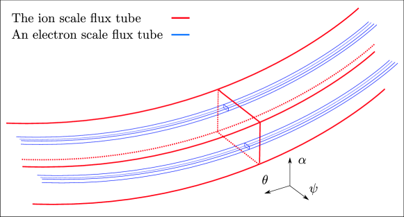
Figure 1: Diagram illustrating how electron scale flux tubes (blue) may be nested within a larger ion scale flux tube (red). The coordinates $(\psi,\alpha,\theta)$ denote the usual magnetic-field-following radial, binormal, and parallel-to-the-field coordinates.

The remainder of the paper is organised as follows. In Section 2 we review the concepts used to derive the gyrokinetic equation that will be necessary for our separation of the ion and electron scales. In Section 3 we state our orderings for length and time scales and present the formalism which we will use to separate the ion and electron scales. We also introduce the method of multiple scales as a technique for deriving the coupled gyrokinetic equations and we define an electron scale average, which, along with the assumption of statistical periodicity of the electron scale turbulence, allows us to uniquely decompose the turbulence into ion and electron scale pieces. In Section 4 we apply the electron scale average to find the coupled ion scale and electron scale gyrokinetic equations, and retain the largest possible cross-scale interaction terms in our expansion in $\left(m_{\rm{e}}/m_{\rm{i}}\right)^{1/2}$. We do this without explicitly assuming the size of the fluctuations, to allow for the possibility of exotic orderings for the sizes of the fluctuations in the presence of cross-scale coupling. In Section 5 we use the electron scale average to find the quasineutrality relations which close the coupled equations. By using dominant balance arguments, we find in Section 6 the only self-consistently-allowed ordering for the size of the ion and electron scale fluctuations: the usual gyro-Bohm ordering. We show that it is possible to neglect the non-adiabatic response of the ion species at electron scales, which is necessary for a local description of the electron scale. In Section 7 we use our results to obtain the maximally-ordered, scale-separated, coupled gyrokinetic equations. At the ion scale we retain the usual ion physics. However, the equation for electrons at ion scales is averaged over the particle orbits in the direction parallel to the magnetic field. The ion scale fluctuations evolve independently of the electron scale turbulence, because there are no cross-scale terms appearing in the ion scale equations. At the electron scale the response of the ion species can be modelled as Maxwell-Boltzmann. The electron equation at electron scales contains two new terms which depend on gradients of ion scale fluctuations. There is an $E\times B$ advection due to the ion scale potential, which varies in the direction parallel to the magnetic field line. The effect of the $E\times B$ advection is to shear electron scale eddies in the parallel-to-the-field direction by differential flows. The gradient of the equilibrium distribution function, the usual drive of instability, is modified by the gradient of the ion scale, electron distribution function. In Section 8 we provide and justify a parallel boundary condition for the electron scale gyrokinetic equation, consistent with the “twist-and-shift” boundary condition [29] for the ion scale turbulence in a local flux tube domain. Finally, in Section 9 we discuss the insights drawn from our scale-separated approach and the physics of the new cross-scale terms that explicitly appear in the coupled equations.

2 The Gyrokinetic Equation

The multi-scale equations that describe the interaction between turbulent fluctuations at ion scales and turbulent fluctuations at electron scales are obtained from the $\delta f$ gyrokinetic equation via an asymptotic expansion in the electron-ion mass ratio. This is a subsidiary expansion within the gyrokinetic ordering [30, 31, 1, 32, 33, 4]. As such, we begin by briefly presenting the steps in the derivation of the $\delta f$ gyrokinetic equation, which describes the evolution of turbulent “fluctuations” around a slowly changing “equilibrium” plasma profile in a plasma which is strongly magnetised. In this paper we only consider electrostatic fluctuations, where we can express the electric field $\bi{E}$ purely in terms of the electrostatic potential $\Phi$, i.e.

$$\bi{E}=-\nabla\Phi.$$ (1)

We specialise to a toroidal geometry. Hence the magnetic field $\bi{B}$ can always be written as

$$\bi{B}=\nabla\alpha\times\nabla\psi,$$ (2)

where the flux label $\psi$ and field line label $\alpha$ will act as our coordinates perpendicular to the field line. We will take the poloidal angle $\theta$ as the coordinate which determines position along the field line.

The $\delta f$ gyrokinetic equation is derived by assuming a separation of space and time scales between the equilibrium profile and fluctuating parts of the particle distribution function. Explicitly, we take

$$\rho_{\rm{th},\nu}/a\rightarrow 0$$ (3)

and

$$\Omega_{\nu}\gg\omega\gg\tau_{\rm{P}}^{-1},$$ (4)

where $a$ is a characteristic equilibrium scale length, $\omega$ is a typical fluctuation frequency and $\tau_{\rm{P}}$ is a characteristic timescale of the equilibrium profiles. It is conventional to order the collision frequency $\nu_{\rm{C}}\sim\omega$ as a maximal ordering to allow for the possibility of both collisionless and collisional plasmas. As the electron-ion mass ratio is treated as an order unity parameter in the gyrokinetic ordering the gyrokinetic equation for each species has the same form. We thus simplify notation by suppressing the species index $\nu$ where it does not introduce ambiguity. We assume that the distribution function $f$ and the electrostatic potential $\Phi$ have negligible amplitude at scales intermediate to $\rho_{\rm{th},\nu}$ and $a$. Moreover, we assume there is no direct cascade of energy between the scales. It is then possible to split the distribution function $f$,

$$f=F+\delta f,$$ (5)

with $F$ and $\delta f$ the equilibrium and fluctuating parts of the distribution function respectively. We introduce a turbulent average $\left\langle{\cdot}\right\rangle^{\mbox{turb}}$, which averages over spatial scales and time scales which are intermediate to the fluctuation and equilibrium scales, such that

$$F=\left\langle{f}\right\rangle^{\mbox{turb}},$$ (6)

with the assumption of statistical periodicity

$$\left\langle{\delta f}\right\rangle^{\mbox{turb}}=0.$$ (7)

Note that (7) can be satisfied by imposing periodicity on the turbulence in the plane perpendicular the magnetic field. This is justified by noting that the turbulent fluctuations should have the same statistics everywhere in a domain that is asymptotically small compared to $a$. This can be ensured by deriving local evolution equations for the turbulence, choosing a simulation domain larger than the correlation length of the turbulence, and imposing periodicity as the boundary condition in the perpendicular domain. We are able to make the assumption of statistical periodicity because of our assumptions of scale separation. This is in contrast to the study of neutral fluids, where the turbulence is universal and the inertial range spans the outer scale to the dissipation scale. As there is no scale-separation in neutral fluids, sub-grid models for neutral fluid turbulence are derived using large eddy simulation (LES) approaches (see e.g. [34, 35, 36]). Let time be $t$, $\nabla$ be the gradient operator, $\bi{b}$ be the unit vector in the direction of the magnetic field, and $\bi{I}$ be the identity matrix. Then $\nabla_{\|}=\bi{b}\cdot\nabla$ is the derivative parallel to the magnetic field, and $\nabla_{\perp}=(\bi{I}-\bi{b}\bi{b})\cdot\nabla$ is the derivative perpendicular to the magnetic field. With these definitions the gyrokinetic orderings for $F$, $\delta f$ and the fluctuating electrostatic potential $\phi$ are

$$\nabla_{\|}F\sim\nabla_{\perp}F\sim\frac{F}{a},\quad\frac{\partial F}{\partial t}\sim\frac{F}{\tau_{\rm{P}}},$$

$$\nabla_{\|}{\delta f}\sim\frac{\delta f}{a},\quad\nabla_{\perp}{\delta f}\sim\frac{\delta f}{\rho_{\rm{th}}},\quad\frac{\partial\delta f}{\partial t}\sim\omega\delta f,$$ (8)

$$\frac{\delta f}{F}\sim\frac{e\phi}{T}\sim\frac{\rho_{\rm{th}}}{a}.$$

The ordering (8) indicates that the fluctuations are highly anisotropic with respect to the magnetic field and evolve rapidly in time compared to the equilibrium.

The gyrokinetic ordering (8) is motivated by particle motion in magnetic confinement fusion devices, which consists of rapid helical motion following magnetic field lines. Particles stream along the field at thermal speed time scales $a/v_{\rm{th}}\sim\omega^{-1}$, which are much longer than the gyration time scale $\Omega^{-1}$, i.e. $\Omega^{-1}\ll a/v_{\rm{th}}$. In order to separate the rapid gyration from the particle streaming it is convenient to use gyrokinetic variables [30, 33] rather than the particle position ${\bi{r}}$ and particle velocity $\bi{v}$. We will use the guiding centre ${\bi{R}}={\bi{r}}-\bm{\rho}_{\nu}$, where $\bm{\rho}_{\nu}=\bi{b}\times\bi{v}/\Omega_{\nu}$ is the vector gyroradius; the particle energy $\varepsilon=m_{\nu}v^{2}/2$, where $v=|\bi{v}|$; the sign of the parallel velocity $\sigma=v_{\|}/|v_{\|}|$, where $v_{\|}=\bi{b}\cdot\bi{v}$; the pitch angle $\lambda=v_{\perp}^{2}/v^{2}B$, where $v_{\perp}=|\bi{v}-v_{\|}\bi{b}|$; and the gyrophase $\gamma$, which identifies the angular position of a particle in its gyromotion, and which is defined by

$$\tan{\gamma}=\frac{\bi{e}_{2}\cdot\bi{v}}{\bi{e}_{1}\cdot\bi{v}},$$ (9)

where $\bi{e}_{1}$ and $\bi{e}_{2}$ are unit vectors which form an orthonormal basis with $\bi{b}$. We define $\bi{e}_{1}$ and $\bi{e}_{2}$ in terms of $\psi$ and $\alpha$ in A. In these variables, variation on $\Omega^{-1}$ time scales occurs only through $\gamma$, over which one can conveniently average. We define the gyroaverage $\left\langle{\cdot}\right\rangle^{\gamma}$ as

$$\left\langle{\cdot}\right\rangle^{\gamma}=\frac{1}{2\pi}\int^{2\pi}_{0}\cdot\;d\gamma.$$ (10)

Note that the gyroaverage is taken at fixed $\varepsilon$, $\sigma$, and $\lambda$. In addition, either ${\bi{r}}$ or ${\bi{R}}$ is held fixed during the gyroaveraging; we will state explicitly whether ${\bi{r}}$ or ${\bi{R}}$ is held fixed in each gyroaverage.

To find equations which determine $\delta f$ and $F$ we use the turbulent average (6), the assumption of statistical periodicity (7), the orderings (8), the gyroaverage (10), and the Fokker-Planck equation for the plasma. We find that the equilibrium piece of the distribution function $F=F_{0}$, where $F_{0}$ is a maxwellian distribution of velocities. The fluctuating piece of the distribution function $\delta f$ is determined by the gyrokinetic equation, which is written in terms of the non-adiabatic response

$$h({\bi{R}},\varepsilon,\lambda,\sigma)=\delta f({\bi{r}},\bi{v})+\frac{Ze\phi({\bi{r}})}{T}F_{0}.$$ (11)

Note that $h$ is independent of $\gamma$ when $h$ is regarded as a function of ${\bi{R}}$. The dependence on $\gamma$ in $\delta f$ arises due to $\bm{\rho}$ in the transformation between ${\bi{r}}$ and ${\bi{R}}$. In terms of $h$, the gyrokinetic equation is

$$\frac{\partial h}{\partial t}+v_{\|}\bi{b}\cdot\nabla\theta\frac{\partial h}{\partial\theta}+(\bi{v}^{M}+\bi{v}^{E})\cdot\nabla h+\bi{v}^{E}\cdot\nabla F_{0}=\frac{ZeF_{0}}{T}\frac{\partial\varphi}{\partial t}+C_{\rm{l}},$$ (12)

where $\varphi=\left\langle{\phi}\right\rangle^{\gamma}_{{\bi{R}}}$ is the gyroaverage of the fluctuating potential at fixed ${\bi{R}}$, $C_{\rm{l}}$ is the gyroaveraged, linearised Fokker-Planck collision operator for the species, $\bi{v}^{M}=(v_{\perp}^{2}/2\Omega)\bi{b}\times\nabla B+(v_{\|}^{2}/\Omega)\bi{b}\times\bi{b}\cdot\nabla\bi{b}$ is the magnetic drift velocity, and

$$\bi{v}^{E}=\frac{c}{B}\bi{b}\times\nabla\varphi$$ (13)

is the gyroaveraged $E\times B$ velocity. To close the gyrokinetic equations for each species one requires an equation for the field; this is the quasineutrality relation,

$$\sum_{\nu}Z_{\nu}e\int d^{3}\bi{v}\big{|}_{\bi{r}}h_{\nu}({\bi{R}},\varepsilon,\lambda,\sigma)=\sum_{\nu}\frac{Z_{\nu}^{2}e^{2}n_{\nu}}{T_{\nu}}\phi({\bi{r}}),$$ (14)

where $n_{\nu}=\int d^{3}\bi{v}F_{0\nu}$ is the equilibrium plasma density. Where it does not introduce ambiguity, we will suppress $({\bi{R}},\varepsilon,\lambda,\sigma)$ dependences and species indices. We will take the collisionless limit $\nu_{\rm{C}}\ll\omega$ in this paper for simplicity; we demonstrate how the effects of collisions may be included within the scale-separated framework in L. It is important to note that in gyrokinetics we implicitly assume that the typical velocity scale of the distribution function for a given species $\delta v_{\nu}\sim v_{\rm{th},\nu}$. In a truly collisionless system $\delta f$ and $F$ could develop arbitrarily small velocity space structures through phase mixing [37, 38, 39, 40, 41, 42, 43, 44], i.e. $\delta v\rightarrow 0$ as $\nu_{\rm{C}}\rightarrow 0$. The presence of the collision operator $C$, a diffusive operator in velocity space, provides the necessary, and physical, regularisation of $\delta f$ and $F$ [45, 46]. In the $\delta f$ gyrokinetic approach, equations (12) and (14) are solved in a field-following domain, termed a flux tube. We use the field-aligned coordinate system $(\psi,\alpha,\theta)$, which is theoretically convenient and allows for an efficient simulation domain which captures the structure of anisotropic, magnetised plasma turbulence with minimal resolution. The flux tube has a narrow extent around a central field line but extends for (typically) a $2\pi$ poloidal circuit along the field line. The assumptions of scale separation in the plane perpendicular to $\bi{B}$, and statistical periodicity (7), permit the use of periodic boundary conditions in the $(\psi,\alpha)$ plane. However, we must also specify a boundary condition in the poloidal angle $\theta$ that gives the location along the magnetic field. The relevant physical boundary condition is periodicity in $\theta$, but this must be applied at fixed toroidal angle $\zeta$ – not at fixed field line label $\alpha$. The presence of shear in the pitch of the magnetic field makes enforcement of this boundary condition non-trivial. The standard flux tube parallel boundary condition is the so-called “twist-and-shift” boundary condition [29].

The gyrokinetic system (12) and (14) is the starting point for our model. Note that the gyrokinetic ordering allows for the possibility that the fluctuations have multiple distinct space and time scales arising from differences in the thermal speed $v_{\rm{th},\nu}$ and thermal gyroradius $\rho_{\rm{th},\nu}$ of each species. Indeed, equilibrium gradients in plasma density and temperature drive instabilities with distinct spatial scales of the ion and electron gyroradii, with corresponding time scales of $a/v_{\rm{th,i}}$ and $a/v_{\rm{th,e}}$, respectively. We suppose the existence of an ion scale (IS) and a separated electron scale (ES) within the turbulence. The separation between the scales is governed by the mass ratio $\left(m_{\rm{e}}/m_{\rm{i}}\right)^{1/2}\sim\rho_{\rm{th,e}}/\rho_{\rm{th,i}}\sim v_{\rm{th,i}}/v_{\rm{th,e}}$, which we treat as an asymptotic expansion parameter; i.e., $\left(m_{\rm{e}}/m_{\rm{i}}\right)^{1/2}\rightarrow 0$. We will assume that fluctuations in the scales intermediate to the IS and ES have vanishing amplitude. Note that our expansion in $\left(m_{\rm{e}}/m_{\rm{i}}\right)^{1/2}$ is a subsidiary expansion within gyrokinetics, so it satisfies $\rho_{\rm{th},\nu}/a\ll\left(m_{\rm{e}}/m_{\rm{i}}\right)^{1/2}$.

We proceed in analogy to the derivation of the coupled equilibrium-fluctuation equations to derive scale-separated, coupled IS-ES equations. These equations contain the physics of nonlocal (in wave number) cross-scale interaction. We propose an extension of the “twist-and-shift” flux tube parallel boundary condition to allow for efficient simulation of the IS-ES equations in a system of coupled flux tubes. We find the IS-ES equations are parallelisable in the sense that the ES equations may be integrated at multiple radial locations within the IS domain without reference to one another.

3 Separation of Scales within the Turbulence

We assume a separation of scales between IS fluctuations and ES fluctuations in the turbulence, i.e., $\left(m_{\rm{e}}/m_{\rm{i}}\right)^{1/2}\rightarrow 0$. We make the assumption that the turbulent fluctuations have negligible amplitude at scales intermediate to the IS and ES. This allows us to decompose the fluctuating distribution function $\delta f$ into

$$\delta f=\overline{\delta f}+\widetilde{\delta f},$$ (15)

where $\overline{\delta f}$ and $\widetilde{\delta f}$ are the fluctuating IS and ES pieces of the particle distribution function, respectively. In order to find evolution equations for $\overline{\delta f}$ and $\widetilde{\delta f}$ we introduce an ES average $\left\langle{\cdot}\right\rangle^{\mbox{ES}}$, which averages over spatial scales and time scales which are intermediate to the IS and ES , such that

$$\left\langle{\delta f}\right\rangle^{\mbox{ES}}=\overline{\delta f},$$ (16)

with the assumption of statistical periodicity

$$\left\langle{\widetilde{\delta f}}\right\rangle^{\mbox{ES}}=0.$$ (17)

This assumption allows us to asymptotically expand the gyrokinetic equation and find unique asymptotic series for $\overline{\delta f}$ and $\widetilde{\delta f}$ in the limit $\left(m_{\rm{e}}/m_{\rm{i}}\right)^{1/2}\rightarrow 0$, and is analogous to the assumption of statistical periodicity (7).

One could derive the coupled multi-scale equations with an implicit assumption of statistical periodicity, as e.g., in [4]. However, here we explicitly show how (17) is satisfied by introducing fast and slow variables for space and time after the method of multiple scales (cf. [47]) and then homogenising the system. This approach clarifies how to deal with the nonlocal nature of gyrokinetics introduced by the gyroaverage.

In analogy to $\delta f$ gyrokinetics, we adopt the following orderings for space and time scales,

$$\nabla_{\parallel}\overline{\delta f}\sim\frac{\overline{\delta f}}{a},\quad\nabla_{\perp}\overline{\delta f}\sim\frac{\overline{\delta f}}{\rho_{\rm{th,i}}},\quad\frac{\partial\overline{\delta f}}{\partial t}\sim\frac{v_{\rm{th,i}}}{a}\overline{\delta f},$$

$$\nabla_{\parallel}\widetilde{\delta f}\sim\frac{\widetilde{\delta f}}{a},\quad\nabla_{\perp}\widetilde{\delta f}\sim\frac{\widetilde{\delta f}}{\rho_{\rm{th,e}}},\quad\frac{\partial\widetilde{\delta f}}{\partial t}\sim\frac{v_{\rm{th,e}}}{a}\widetilde{\delta f}.$$ (18)

Note that we assume that the parallel scale is always set by the machine size, and hence we do not assume separation of scales in the parallel direction. These assumptions will be justified a posteriori using a critical balance argument. Our ordering (18) assumes spatial isotropy in the turbulence in the plane perpendicular to the magnetic field line; this assumption excludes structures which have scales of size $\rho_{\rm{th,i}}$ in one direction perpendicular to the magnetic field, but scales of size $\rho_{\rm{th,e}}$ in another. In particular, this assumption excludes electron temperature gradient (ETG) streamers [11, 12, 13] if their radial extent scales like $\rho_{\rm{th,i}}$ rather than $\rho_{\rm{th,e}}$. Using the orderings (18) we proceed to find coupled IS-ES equations including all terms which might be relevant to leading order. We then use dominant balance arguments to find orderings for the size of the fluctuations consistent with (18), and neglect the terms in the coupled IS-ES equations which are small.

We introduce a fast spatial variable ${\bi{r}_{\rm{f}}}$ and a slow spatial variable ${\bi{r}_{\rm{s}}}$ in the 2-D plane perpendicular to the field line, such that all ES variation in the solution appears through dependence on ${\bi{r}_{\rm{f}}}$, and all IS variation appears through dependence on ${\bi{r}_{\rm{s}}}$. Functions of ${\bi{r}}$ will become functions of $(\theta,{\bi{r}_{\rm{s}}},{\bi{r}_{\rm{f}}})$, where the perpendicular and parallel spatial dependence is explicitly written out. We will also introduce fast and slow guiding centre coordinates, ${\bi{R}_{\rm{f}}}={\bi{r}_{\rm{f}}}-\bm{\rho}_{\nu}$ and ${\bi{R}_{\rm{s}}}={\bi{r}_{\rm{s}}}-\bm{\rho}_{\nu}$, respectively. We introduce the fast and slow times ${t_{\rm{f}}}$ and ${t_{\rm{s}}}$, respectively. Functions of $t$ will become functions of $({t_{\rm{s}}},{t_{\rm{f}}})$. Note that the slow variables do not contain equilibrium variation, as this is ordered out in deriving the gyrokinetic equation. We will assume periodicity of the fluctuations in ${\bi{r}_{\rm{s}}}$ to be consistent with the separation of scales between the fluctuations and the equilibrium assumed in $\delta f$ gyrokinetics via condition (7). The gyrokinetic equation must be modified so that,

$$\delta f(t,{\bi{r}})\rightarrow\delta f({t_{\rm{s}}},{t_{\rm{f}}},\theta,{\bi{r}_{\rm{s}}},{\bi{r}_{\rm{f}}}),$$ (19)

$$\nabla_{\perp}\rightarrow\nabla_{\rm{s}}+\nabla_{\rm{f}},\quad\nabla_{\rm{s}}\sim\rho_{\rm{th,i}}^{-1},\quad\nabla_{\rm{f}}\sim\rho_{\rm{th,e}}^{-1},$$ (20)

$$\frac{\partial}{\partial t}\rightarrow\frac{\partial}{\partial{t_{\rm{s}}}}+\frac{\partial}{\partial{t_{\rm{f}}}},\quad\frac{\partial}{\partial{t_{\rm{s}}}}\sim\frac{v_{\rm{th,i}}}{a},\quad\frac{\partial}{\partial{t_{\rm{f}}}}\sim\frac{v_{\rm{th,e}}}{a}.$$ (21)

We then perform an asymptotic expansion on the resulting equations in the mass ratio $\left(m_{\rm{e}}/m_{\rm{i}}\right)^{1/2}$ to find the leading order, asymptotically valid equations. With the introduction of the new variables we may explicitly define the ES average,

$$\overline{\delta f}({t_{\rm{s}}},\theta,{\bi{r}_{\rm{s}}})=\left\langle{\delta f({t_{\rm{s}}},{t_{\rm{f}}},\theta,{\bi{r}_{\rm{s}}},{\bi{r}_{\rm{f}}})}\right\rangle^{\mbox{ES}}=$$

$$\frac{1}{\tau_{\rm{c}}A_{\rm{e}}}\int^{{t_{\rm{s}}}+\tau_{\rm{c}}/2}_{{t_{\rm{s}}}-\tau_{\rm{c}}/2}d{t_{\rm{f}}}\int^{\psi_{\rm{s}}+\Delta_{\psi}/2}_{\psi_{\rm{s}}-\Delta_{\psi}/2}d\psi_{\rm{f}}\int^{\alpha_{\rm{s}}+\Delta_{\alpha}/2}_{\alpha_{\rm{s}}-\Delta_{\alpha}/2}d\alpha_{\rm{f}}\;\mathcal{J}\;\delta f({t_{\rm{s}}},{t_{\rm{f}}},\theta,{\bi{r}_{\rm{s}}},{\bi{r}_{\rm{f}}}),$$ (22)

where $\tau_{\rm{c}}$ is a time intermediate to the ES and IS correlation times; $\Delta_{\psi}$ and $\Delta_{\alpha}$ are intermediate to the ES and IS correlation lengths and angles in the $\psi$ and $\alpha$ directions, respectively; $\psi_{\rm{f}}$ and $\psi_{\rm{s}}$ are the fast and slow flux labels, respectively; $\alpha_{\rm{f}}$ and $\alpha_{\rm{s}}$ are the fast and slow field line labels, respectively; $\mathcal{J}$ is the Jacobian of the transformation from ${\bi{r}_{\rm{f}}}\rightarrow(\psi_{\rm{f}},\alpha_{\rm{f}})$, and

$$A_{\rm{e}}=\int^{\psi_{\rm{s}}+\Delta_{\psi}/2}_{\psi_{\rm{s}}-\Delta_{\psi}/2}d\psi_{\rm{f}}\int^{\alpha_{\rm{s}}+\Delta_{\alpha}/2}_{\alpha_{\rm{s}}-\Delta_{\alpha}/2}d\alpha_{\rm{f}}\;\mathcal{J}.$$ (23)

Note that we regard ${\bi{r}_{\rm{f}}}={\bi{r}_{\rm{f}}}(\psi_{\rm{f}},\alpha_{\rm{f}})$ and ${\bi{r}_{\rm{s}}}={\bi{r}_{\rm{s}}}(\psi_{\rm{s}},\alpha_{\rm{s}})$ in the integration in (22) and (23). To satisfy (17) for every $({t_{\rm{s}}},\theta,{\bi{r}_{\rm{s}}})$, we impose that the fluctuations are periodic in the fast variable ${\bi{r}_{\rm{f}}}$. In particular we assume that

$$\delta f({t_{\rm{s}}},{t_{\rm{f}}},\theta,{\bi{r}_{\rm{s}}},{\bi{r}_{\rm{f}}})=\delta f({t_{\rm{s}}},{t_{\rm{f}}},\theta,{\bi{r}_{\rm{s}}},{\bi{r}_{\rm{f}}}+j\Delta_{\psi}\bi{e}_{\psi}+l\Delta_{\alpha}\bi{e}_{\alpha}),$$ (24)

where $j$, $l$ are any integers, $\bi{e}_{\psi}=(\bi{b}\times\nabla\alpha)/|\nabla\psi\cdot\bi{b}\times\nabla\alpha|$, and $\bi{e}_{\alpha}=(\nabla\psi\times\bi{b})/|\nabla\psi\cdot\bi{b}\times\nabla\alpha|$.

The ES average (22) is an average over areas perpendicular to the magnetic field line, and times intermediate to $a/v_{\rm{th,i}}$ and $a/v_{\rm{th,e}}$, with the average taken at fixed $\theta$, $\varepsilon$, $\lambda$, and $\sigma$. To find the scale-separated, leading order equation for electrons at IS it is also necessary to average the IS electron gyrokinetic equation over electron orbits parallel to the magnetic field line, cf.[48]. This necessity arises because electron parallel streaming, which introduces frequencies of order $v_{\rm{th,e}}/a$, is faster than any other IS dynamics, which by assumption have frequencies of order $v_{\rm{th,i}}/a\ll v_{\rm{th,e}}/a$. Naively this would appear to break our ordering, as it would seem we would need to include ES timescales in the IS equation. Furthermore, it is known that rapid electron streaming can lead to very long tails in ballooning modes due to the passing electron response [49]. The long ballooning tails result in very fine radial structure in the turbulence near low order mode rational surfaces [50]. This problem is resolved by treating electron parallel streaming at IS as being asymptotically faster than IS frequencies, consistent with our expansion. To find the leading order equation for the electron distribution function at IS we introduce the orbital average $\left\langle{\cdot}\right\rangle^{\rm{o}}$. After [51] we define the orbital average $\left\langle{\cdot}\right\rangle^{\rm{o}}$ in the passing and trapped parts of velocity space separately. In the passing region of velocity space

$$\left\langle{\cdot}\right\rangle^{\rm{o}}=\frac{\int d\alpha_{\rm{s}}d\theta\;\cdot/v_{\|}\bi{b}\cdot\nabla\theta}{\int d\alpha_{\rm{s}}d\theta/v_{\|}\bi{b}\cdot\nabla\theta},$$ (25)

where the integration $\int d\alpha_{\rm{s}}d\theta$ is taken over the whole flux surface. In the trapped region of velocity space

$$\left\langle{\cdot}\right\rangle^{\rm{o}}=\frac{\sum_{\sigma}\int^{\theta^{+}}_{\theta^{-}}d\theta\;\cdot/|v_{\|}|\bi{b}\cdot\nabla\theta}{2\int^{\theta^{+}}_{\theta^{-}}d\theta/|v_{\|}|\bi{b}\cdot\nabla\theta},$$ (26)

where the limits in the integration $\theta^{+}$ and $\theta^{-}$ are the upper and lower bounce points of the trapped particle, respectively. Note that the orbital average commutes with fast and slow spatial derivatives,

$$\nabla_{\rm{s}}\left\langle{\cdot}\right\rangle^{\rm{o}}=\left\langle{\nabla_{\rm{s}}\cdot}\right\rangle^{\rm{o}}$$ (27)

and

$$\nabla_{\rm{f}}\left\langle{\cdot}\right\rangle^{\rm{o}}=\left\langle{\nabla_{\rm{f}}\cdot}\right\rangle^{\rm{o}}$$ (28)

as $v_{\|}\bi{b}\cdot\nabla\theta$ contains only equilibrium spatial variation. With the definitions (25) and (26) we show in C.1 that the orbital average $\left\langle{\cdot}\right\rangle^{\rm{o}}$ has the very useful property

$$\left\langle{v_{\|}\bi{b}\cdot\nabla\theta\frac{\partial H}{\partial\theta}}\right\rangle^{\rm{o}}=0$$ (29)

for any $H(\theta,{\bi{R}_{\rm{s}}},\varepsilon,\lambda,\sigma)$. The property (29) will allow us to use the orbital average $\left\langle{\cdot}\right\rangle^{\rm{o}}$ to eliminate parallel streaming from the electron equation at IS.

4 Coupled Gyrokinetic Equations

In this Section we will use the ideas of Section 3 to find the scale-separated IS and ES gyrokinetic equations, where the largest possible cross-scale terms are retained. We take this approach, as it will allow us to consider whether or not the presence of cross-scale interaction can lead to novel mass ratio orderings for the sizes of the fluctuations.

We now apply the ES average (22) to the gyrokinetic equation (12) to find the IS gyrokinetic equation. The resulting gyrokinetic equation is a function of ${\bi{R}_{\rm{s}}}$. We suppress species indices, but note that what is done here applies to both ion and electron species. Upon averaging, the gyrokinetic equation is,

$$\frac{\partial\overline{h}}{\partial{t_{\rm{s}}}}+v_{\|}\bi{b}\cdot\nabla\theta\frac{\partial\overline{h}_{\rm{i}}}{\partial\theta}+\bi{v}^{M}\cdot\nabla_{\rm{s}}\overline{h}+\left\langle{\bi{v}^{E}\cdot\nabla h}\right\rangle^{\mbox{ES}}+\overline{\bi{v}}^{E}\cdot\nabla F_{0}=\frac{ZeF_{0}}{T}\frac{\partial\overline{\varphi}}{\partial{t_{\rm{s}}}},$$ (30)

where

$$\overline{\bi{v}}^{E}=\frac{c}{B}\bi{b}\times\nabla_{\rm{s}}\overline{\varphi},$$ (31)

and

$$\overline{\varphi}=\left\langle{\overline{\phi}}\right\rangle^{\gamma}_{{\bi{R}_{\rm{s}}}}=\left\langle{\left\langle{\phi}\right\rangle^{\mbox{ES}}}\right\rangle^{\gamma}_{{\bi{R}_{\rm{s}}}}.$$ (32)

Note that whilst the gyroaveraged potential $\varphi$ is a function of ${\bi{R}_{\rm{f}}}$, the potential $\phi$ is a function of ${\bi{r}_{\rm{f}}}$. To obtain (30)-(32), we used the fact that the the ES average can be taken over either the real space variable ${\bi{r}_{\rm{f}}}$ or the guiding centre ${\bi{R}_{\rm{f}}}$, and that the ES average commutes with the gyroaverage,

$$\left\langle{\left\langle{\cdot}\right\rangle^{\mbox{ES}}}\right\rangle^{\gamma}_{{\bi{R}_{\rm{f}}},{\bi{R}_{\rm{s}}}}=\left\langle{\left\langle{\cdot}\right\rangle^{\gamma}_{{\bi{R}_{\rm{f}}},{\bi{R}_{\rm{s}}}}}\right\rangle^{\mbox{ES}},$$ (33)

where the notation $\left\langle{\cdot}\right\rangle^{\gamma}_{{\bi{R}_{\rm{f}}},{\bi{R}_{\rm{s}}}}$ indicates a gyroaverage with both ${\bi{R}_{\rm{f}}}$ and ${\bi{R}_{\rm{s}}}$ held fixed. Both of these properties are proven in B. The linear terms in (30) are simply filtered versions of the terms in the $\delta f$ gyrokinetic equation (12). However, the nonlinear term yields a new, cross-scale coupling term. As shown in D.1, the form of this new term is

$$\left\langle{\bi{v}^{E}\cdot\nabla h}\right\rangle^{\mbox{ES}}=\overline{\bi{v}}^{E}\cdot\nabla_{\rm{s}}\overline{h}+\nabla_{\rm{s}}\cdot\left\langle{\tilde{h}\frac{c}{B}\bi{b}\times(\nabla_{\rm{s}}+\nabla_{\rm{f}})\tilde{\varphi}}\right\rangle^{\mbox{ES}},$$

where $\overline{\bi{v}}^{E}\cdot\nabla_{\rm{s}}\overline{h}$ is the usual $E\times B$ nonlinearity appearing in the IS gyrokinetic equation in the absence of cross-scale coupling. Dropping the $\nabla_{\rm{s}}\tilde{\varphi}$ term since it is a factor $\left(m_{\rm{e}}/m_{\rm{i}}\right)^{1/2}$ smaller than the $\nabla_{\rm{f}}\tilde{\varphi}$ term, we find

$$\left\langle{\bi{v}^{E}\cdot\nabla h}\right\rangle^{\mbox{ES}}=\overline{\bi{v}}^{E}\cdot\nabla_{\rm{s}}\overline{h}+\nabla_{\rm{s}}\cdot\left\langle{\tilde{\bi{v}}^{E}\tilde{h}}\right\rangle^{\mbox{ES}},$$ (34)

where

$$\tilde{\bi{v}}^{E}=\frac{c}{B}\bi{b}\times\nabla_{\rm{f}}\tilde{\varphi}.$$ (35)

After filtering with the ES average, the IS equations for ions and electrons in the presence of cross-scale coupling are therefore

$$\frac{\partial\overline{h}_{\rm{i}}}{\partial{t_{\rm{s}}}}+v_{\|}\bi{b}\cdot\nabla\theta\frac{\partial\overline{h}_{\rm{i}}}{\partial\theta}+\bi{v}^{M}_{\rm{i}}\cdot\nabla_{\rm{s}}\overline{h}+\overline{\bi{v}}^{E}_{\rm{i}}\cdot\nabla_{\rm{s}}\overline{h}_{\rm{i}}$$

$$+\nabla_{\rm{s}}\cdot\left\langle{\tilde{\bi{v}}^{E}_{\rm{i}}\tilde{h}_{\rm{i}}}\right\rangle^{\mbox{ES}}+\overline{\bi{v}}^{E}_{\rm{i}}\cdot\nabla F_{0i}=\frac{Z_{\rm{i}}eF_{0i}}{T}\frac{\partial\overline{\varphi}_{\rm{i}}}{\partial{t_{\rm{s}}}},$$ (36)

and

$$\frac{\partial\overline{h}_{\rm{e}}}{\partial{t_{\rm{s}}}}+v_{\|}\bi{b}\cdot\nabla\theta\frac{\partial\overline{h}_{\rm{e}}}{\partial\theta}+\bi{v}^{M}_{\rm{e}}\cdot\nabla_{\rm{s}}\overline{h}_{\rm{e}}+\overline{\bi{v}}^{E}_{\rm{e}}\cdot\nabla_{\rm{s}}\overline{h}_{\rm{e}}$$

$$+\nabla_{\rm{s}}\cdot\left\langle{\tilde{\bi{v}}^{E}_{\rm{e}}\tilde{h}_{\rm{e}}}\right\rangle^{\mbox{ES}}+\overline{\bi{v}}^{E}_{\rm{e}}\cdot\nabla F_{0e}=-\frac{eF_{0e}}{T}\frac{\partial\overline{\varphi}_{\rm{e}}}{\partial{t_{\rm{s}}}}.$$ (37)

The only modifications to the usual IS gyrokinetic equations are the inclusion of $\nabla_{\rm{s}}\cdot\left\langle{\tilde{\bi{v}}^{E}_{\rm{i}}\tilde{h}_{\rm{i}}}\right\rangle^{\mbox{ES}}$ in (36), and $\nabla_{\rm{s}}\cdot\left\langle{\tilde{\bi{v}}^{E}_{\rm{e}}\tilde{h}_{\rm{e}}}\right\rangle^{\mbox{ES}}$ in (37). The terms $\nabla_{\rm{s}}\cdot\left\langle{\tilde{\bi{v}}^{E}_{\rm{i}}\tilde{h}_{\rm{i}}}\right\rangle^{\mbox{ES}}$ and $\nabla_{\rm{s}}\cdot\left\langle{\tilde{\bi{v}}^{E}_{\rm{e}}\tilde{h}_{\rm{e}}}\right\rangle^{\mbox{ES}}$ physically represent the divergence of the spatial fluxes of $\overline{h}_{\rm{i}}$ and $\overline{h}_{\rm{e}}$ due to ES fluctuations. The reader will notice that (37) contains electron parallel streaming $v_{\|}\bi{b}\cdot\nabla\theta{\partial\overline{h}_{\rm{e}}}/{\partial\theta}$. As a consequence, equation (37) is not properly scale-separated, as the equation still contains $a/v_{\rm{th,e}}$ time scales and $\rho_{\rm{th,e}}$ spatial scales. In our asymptotic expansion the leading order equation for electrons at IS is

$$v_{\|}\bi{b}\cdot\nabla\theta\frac{\partial\overline{h}_{\rm{e}}}{\partial\theta}=0.$$ (38)

To solve this equation we decompose

$$\overline{h}_{\rm{e}}=\overline{h}_{\rm{e}}^{(0)}({\bi{R}_{\rm{s}}},\varepsilon,\lambda,\sigma)+\overline{h}_{\rm{e}}^{(1)}(\theta,{\bi{R}_{\rm{s}}},\varepsilon,\lambda,\sigma),$$ (39)

where $\overline{h}_{\rm{e}}^{(0)}\sim e\overline{\phi}/T$ and $\overline{h}_{\rm{e}}^{(1)}\sim\left(m_{\rm{e}}/m_{\rm{i}}\right)^{1/2}\overline{h}_{\rm{e}}^{(0)}$. Note $\overline{h}_{\rm{e}}^{(0)}$ has no dependence on $\theta$. We see that if we explicitly make the decomposition (39) when solving (37) then we can formally order

$$v_{\|}\bi{b}\cdot\nabla\theta\frac{\partial\overline{h}_{\rm{e}}}{\partial\theta}=v_{\|}\bi{b}\cdot\nabla\theta\frac{\partial\overline{h}_{\rm{e}}^{(1)}}{\partial\theta}\sim\frac{v_{\rm{th,i}}}{a}\overline{h}_{\rm{e}}^{(0)}\sim\bi{v}^{M}_{\rm{e}}\cdot\nabla_{\rm{s}}\overline{h}_{\rm{e}}.$$ (40)

We take only the leading order piece of the electron distribution function $\overline{h}_{\rm{e}}=\overline{h}_{\rm{e}}^{(0)}$. Defining the non-zonal piece of the distribution function to be the piece which contains variation in $\alpha_{\rm{s}}$, we show in C.2 that $\overline{h}_{\rm{e}}^{(0)}=0$ for the non-zonal passing piece of the electron distribution function. This is a result of the usual “twist-and-shift” boundary condition [29] which connects modes of different radial wavenumber, with the observation that modes which have very high radial wavenumber should have $h\rightarrow 0$. To obtain the equation for the non-zero piece of $\overline{h}_{\rm{e}}^{(0)}$ we need to eliminate the parallel streaming term $v_{\|}\bi{b}\cdot\nabla\theta{\partial\overline{h}_{\rm{e}}^{(1)}}/{\partial\theta}$ from (37). We achieve this by averaging over the rapid parallel orbits of the electrons in (37). We use the orbital average, defined in (25) and (26), and the properties (29),

$$\left\langle{\overline{h}_{\rm{e}}^{(0)}}\right\rangle^{\rm{o}}=\overline{h}_{\rm{e}}^{(0)}$$ (41)

and [52, 53]

$$\left\langle{\bi{v}^{M}\cdot\nabla\psi}\right\rangle^{\rm{o}}=0,$$ (42)

shown in C.3. The resulting, scale-separated, equation for the leading order piece of the electron distribution function at IS, $\overline{h}_{\rm{e}}=\overline{h}_{\rm{e}}^{(0)}$, is

$$\frac{\partial\overline{h}_{\rm{e}}}{\partial{t_{\rm{s}}}}+\left\langle{\bi{v}^{M}_{\rm{e}}\cdot\nabla\alpha}\right\rangle^{\rm{o}}\frac{\partial\overline{h}_{\rm{e}}}{\partial\alpha_{\rm{s}}}+\left\langle{\overline{\bi{v}}^{E}_{\rm{e}}\cdot\nabla_{\rm{s}}\overline{h}_{\rm{e}}}\right\rangle^{\rm{o}}+\left\langle{\overline{\bi{v}}^{E}_{\rm{e}}\cdot\nabla F_{0e}}\right\rangle^{\rm{o}}$$

$$+\nabla_{\rm{s}}\cdot\left\langle{\left\langle{\tilde{\bi{v}}^{E}_{\rm{e}}\tilde{h}_{\rm{e}}}\right\rangle^{\mbox{ES}}}\right\rangle^{\rm{o}}=-\frac{eF_{0e}}{T_{\rm{e}}}\frac{\partial\left\langle{\overline{\varphi}_{\rm{e}}}\right\rangle^{\rm{o}}}{\partial{t_{\rm{s}}}},$$ (43)

where it is understood that $\overline{h}_{\rm{e}}=0$ for the non-zonal passing piece of the electron distribution function.

To find the ES equation we subtract the IS equation (30) from the full equation (12). Again, the linear terms follow easily and the nonlinear term provides new cross-scale coupling terms:

$$\frac{\partial\tilde{h}}{\partial{t_{\rm{s}}}}+\frac{\partial\tilde{h}}{\partial{t_{\rm{f}}}}+v_{\|}\bi{b}\cdot\nabla\theta\frac{\partial\tilde{h}}{\partial\theta}+\bi{v}^{M}\cdot(\nabla_{\rm{s}}+\nabla_{\rm{f}})\tilde{h}+\left[\bi{v}^{E}\cdot\nabla h-\left\langle{\bi{v}^{E}\cdot\nabla h}\right\rangle^{\mbox{ES}}\right]$$

$$+\left(\frac{c}{B}\bi{b}\times\left(\nabla_{\rm{s}}+\nabla_{\rm{f}}\right)\tilde{\varphi}\right)\cdot\nabla F_{0}=\frac{ZeF_{0}}{T}\left(\frac{\partial\tilde{\varphi}}{\partial{t_{\rm{s}}}}+\frac{\partial\tilde{\varphi}}{\partial{t_{\rm{f}}}}\right).$$ (44)

We can further simplify (44) by neglecting sub-dominant terms in $\left(m_{\rm{e}}/m_{\rm{i}}\right)^{1/2}$; i.e., $\nabla_{\rm{s}}+\nabla_{\rm{f}}\approx\nabla_{\rm{f}}$, $\partial/\partial t_{s}+\partial/\partial t_{f}\approx\partial/\partial t_{f}$, and $v_{\|}\bi{b}\cdot\nabla\theta{\partial\tilde{h}_{\rm{i}}}/{\partial\theta}\ll\bi{v}^{M}\cdot\nabla_{\rm{f}}\tilde{h}_{\rm{i}}$ in the equation for ions. As shown in D.2, the nonlinear term reduces to

$$\bi{v}^{E}\cdot\nabla h-\left\langle{\bi{v}^{E}\cdot\nabla h}\right\rangle^{\mbox{ES}}=\tilde{\bi{v}}^{E}\cdot\nabla_{\rm{f}}\tilde{h}+\overline{\bi{v}}^{E}\cdot\nabla_{\rm{f}}\tilde{h}+\tilde{\bi{v}}^{E}\cdot\nabla_{\rm{s}}\overline{h},$$ (45)

where $\tilde{\bi{v}}^{E}\cdot\nabla_{\rm{f}}\tilde{h}$ is the usual $E\times B$ nonlinearity appearing in the ES gyrokinetic equation in the absence of cross-scale coupling. Combining these results, the ES equation (44), for electrons, becomes

$$\frac{\partial\tilde{h}_{\rm{e}}}{\partial{t_{\rm{f}}}}+v_{\|}\bi{b}\cdot\nabla\theta\frac{\partial\tilde{h}_{\rm{e}}}{\partial\theta}+(\bi{v}^{M}_{\rm{e}}+\overline{\bi{v}}^{E}_{\rm{e}})\cdot\nabla_{\rm{f}}\tilde{h}_{\rm{e}}$$

$$+\tilde{\bi{v}}^{E}_{\rm{e}}\cdot\nabla_{\rm{f}}\tilde{h}_{\rm{e}}+\tilde{\bi{v}}^{E}_{\rm{e}}\cdot(\nabla F_{0e}+\nabla_{\rm{s}}\overline{h}_{\rm{e}})=-\frac{eF_{0e}}{T}\frac{\partial\tilde{\varphi}_{\rm{e}}}{\partial{t_{\rm{f}}}}.$$ (46)

For ions, equation (44) becomes

$$\frac{\partial\tilde{h}_{\rm{i}}}{\partial{t_{\rm{f}}}}+(\bi{v}^{M}_{\rm{i}}+\overline{\bi{v}}^{E}_{\rm{i}})\cdot\nabla_{\rm{f}}\tilde{h}_{\rm{i}}+\tilde{\bi{v}}^{E}_{\rm{i}}\cdot\nabla_{\rm{f}}\tilde{h}_{\rm{i}}+\tilde{\bi{v}}^{E}_{\rm{i}}\cdot(\nabla F_{0i}+\nabla_{\rm{s}}\overline{h}_{\rm{i}})=\frac{Z_{\rm{i}}eF_{0i}}{T}\frac{\partial\tilde{\varphi}_{\rm{i}}}{\partial{t_{\rm{f}}}}.$$ (47)

Equations (46) and (47) contain the effect of IS gradients on ES fluctuations through two terms: $\overline{\bi{v}}^{E}\cdot\nabla_{\rm{f}}\tilde{h}$, which represents advection of ES fluctuations by IS eddies; and $\tilde{\bi{v}}^{E}\cdot\nabla_{\rm{s}}\overline{h}$, which represents the modification of the equilibrium gradient drive due to gradients in the IS fluctuations. Note that the term $\overline{\bi{v}}^{E}\cdot\nabla_{\rm{f}}\tilde{h}$ cannot be eliminated by a change of reference frame because the advection velocity $\overline{\bi{v}}^{E}$ is a function of the parallel-to-the-field coordinate $\theta$, as $\overline{\phi}$ varies along the magnetic field line. The ES equations (46) and (47) are scale-separated in the sense that ${\bi{R}_{\rm{s}}}$ appears only as a label of the IS gradients $\nabla_{\rm{s}}\overline{\varphi}({\bi{R}_{\rm{s}}})$ and $\nabla_{\rm{s}}\overline{h}({\bi{R}_{\rm{s}}})$, and as a label on the fields $\tilde{\varphi}({\bi{R}_{\rm{s}}},{\bi{R}_{\rm{f}}})$ and $\tilde{h}({\bi{R}_{\rm{s}}},{\bi{R}_{\rm{f}}})$.

5 Quasineutrality

Using (16) and (33), and noting that the integration variable for the ES average can be either ${\bi{r}_{\rm{f}}}$, or ${\bi{R}_{\rm{f}}}$ (see B), one can directly find the IS quasineutrality relation,

$$\sum_{\nu}Z_{\nu}e\int d^{3}\bi{v}|_{\bi{r}_{\rm{s}}}\overline{h}_{\nu}(\theta,{\bi{R}_{\rm{s}}},\varepsilon,\lambda,\sigma)=\sum_{\nu}\frac{Z_{\nu}^{2}e^{2}n_{\nu}}{T_{\nu}}\overline{\phi}(\theta,{\bi{r}_{\rm{s}}}),$$ (48)

which is supplemented by the relation,

$$\overline{\varphi}=\left\langle{\overline{\phi}}\right\rangle^{\gamma}_{{\bi{R}_{\rm{s}}}}.$$ (49)

We find the quasineutrality relation for the ES by subtracting (48) from the full quasineutrality relation (14) to obtain,

$$\sum_{\nu}Z_{\nu}e\int d^{3}\bi{v}|_{{\bi{r}_{\rm{s}}},{\bi{r}_{\rm{f}}}}\tilde{h}_{\nu}(\theta,{\bi{R}_{\rm{s}}},{\bi{R}_{\rm{f}}},\varepsilon,\lambda,\sigma)=\sum_{\nu}\frac{Z_{\nu}^{2}e^{2}n_{\nu}}{T_{\nu}}\tilde{\phi}(\theta,{\bi{r}_{\rm{s}}},{\bi{r}_{\rm{f}}}),$$ (50)

which is supplemented by the relation,

$$\tilde{\varphi}=\left\langle{\tilde{\phi}}\right\rangle^{\gamma}_{{\bi{R}_{\rm{f}}},{\bi{R}_{\rm{s}}}}.$$ (51)

The system of equations (36), (43), and (46)-(51) constitutes a formally closed system of equations for the IS and ES quantities. To calculate the ion contribution to the ES quasineutrality relation (50) requires that we take a gyroaverage over a scale of the ion gyroradius, as does computing the ion gyroaveraged potential $\tilde{\varphi}_{\rm{i}}$ in equation (51). Naively one might think that the ion species would thus introduce ion gyroradius scale correlations in the ES turbulence. However, by considering the possible dominant balances in the IS-ES system we will find the contributions from ions at ES can always be ignored, and so we will arrive at a fully scale-separated system.

6 Sizes of the IS and ES fluctuations and scale-separation

We now proceed to find all possible self-consistent orderings for $\overline{h}_{\rm{i}}$, $\overline{h}_{\rm{e}}$, $\tilde{h}_{\rm{i}}$, $\tilde{h}_{\rm{e}}$, $\overline{\phi}$, and $\tilde{\phi}$ that lead to steady-state solutions to the system of equations (36), (43), and (46)-(51). For a statistically steady-state turbulence to be possible there must be a competition between the growth of linear instabilities and nonlinear interactions, which can be cross-scale in nature. We look for dominant balances consistent with this observation.

Note that the presence of the gyroaverages can introduce mass ratio factors. Recalling that we have periodicity perpendicular to the field line in both the slow and fast variables, we write a fluctuation $\phi({\bi{r}_{\rm{s}}},{\bi{r}_{\rm{f}}})$ as,

$$\phi({\bi{r}_{\rm{s}}},{\bi{r}_{\rm{f}}})=\sum_{{\bi{k}_{\rm{f}}}}\phi_{{\bi{k}_{\rm{f}}}}({\bi{r}_{\rm{s}}})\exp{[\rmi{\bi{k}_{\rm{f}}}\cdot{\bi{r}_{\rm{f}}}]}=\sum_{{\bi{k}_{\rm{f}}},{\bi{k}_{\rm{s}}}}\phi_{{\bi{k}_{\rm{f}}},{\bi{k}_{\rm{s}}}}\exp{[\rmi{\bi{k}_{\rm{f}}}\cdot{\bi{r}_{\rm{f}}}]}\exp{[\rmi{\bi{k}_{\rm{s}}}\cdot{\bi{r}_{\rm{s}}}]},$$ (52)

where ${\bi{k}_{\rm{f}}}\sim\rho_{\rm{th,e}}^{-1}$, ${\bi{k}_{\rm{s}}}\sim\rho_{\rm{th,i}}^{-1}$, and we have used periodicity in ${\bi{r}_{\rm{s}}}$ to write $\phi_{{\bi{k}_{\rm{f}}}}({\bi{r}_{\rm{s}}})=\sum_{{\bi{k}_{\rm{s}}}}\phi_{{\bi{k}_{\rm{f}}},{\bi{k}_{\rm{s}}}}\exp{[\rmi{\bi{k}_{\rm{s}}}\cdot{\bi{r}_{\rm{s}}}]}$. If we gyroaverage (52), recalling ${\bi{R}_{\rm{f}}}={\bi{r}_{\rm{f}}}-\bm{\rho}$ and ${\bi{R}_{\rm{s}}}={\bi{r}_{\rm{s}}}-\bm{\rho}$, we find

$$\left\langle{\phi({\bi{r}_{\rm{s}}},{\bi{r}_{\rm{f}}})}\right\rangle^{\gamma}_{{\bi{R}_{\rm{f}}},{\bi{R}_{\rm{s}}}}=\sum_{{\bi{k}_{\rm{f}}},{\bi{k}_{\rm{s}}}}\phi_{{\bi{k}_{\rm{f}}},{\bi{k}_{\rm{s}}}}\exp{[\rmi{\bi{k}_{\rm{f}}}\cdot{\bi{R}_{\rm{f}}}]}\exp{[\rmi{\bi{k}_{\rm{s}}}\cdot{\bi{R}_{\rm{s}}}]}\left\langle{\exp{[\rmi({\bi{k}_{\rm{f}}}+{\bi{k}_{\rm{s}}})\cdot\bm{\rho}]}}\right\rangle^{\gamma}$$

$$=\sum_{{\bi{k}_{\rm{f}}},{\bi{k}_{\rm{s}}}}\phi_{{\bi{k}_{\rm{f}}},{\bi{k}_{\rm{s}}}}\exp{[\rmi{\bi{k}_{\rm{f}}}\cdot{\bi{R}_{\rm{f}}}]}\exp{[\rmi{\bi{k}_{\rm{s}}}\cdot{\bi{R}_{\rm{s}}}]}J_{0}(|{\bi{k}_{\rm{f}}}+{\bi{k}_{\rm{s}}}||\bm{\rho}|),$$ (53)

where $J_{0}(z)$ is the 0th Bessel function of the 1st kind, and we used the result

$$\left\langle{\exp{[\rmi\bi{k}\cdot\bm{\rho}]}}\right\rangle^{\gamma}=J_{0}(|\bi{k}||\bm{\rho}|),$$ (54)

shown in A. Note that $J_{0}(z)\sim 1$ for $z\lesssim 1$ and $J_{0}(z)\sim z^{-1/2}$ for $z\gg 1$. Because $|{\bi{k}_{\rm{f}}}|\rho_{\rm{th,e}}\sim|{\bi{k}_{\rm{s}}}|\rho_{\rm{th,i}}\sim 1$ and $|{\bi{k}_{\rm{s}}}|\rho_{\rm{th,e}}\sim\left(m_{\rm{e}}/m_{\rm{i}}\right)^{1/2}\ll 1$, the gyroaverage introduces no additional mass ratio factors for IS quantities or for electrons at electron scales. However, because $|{\bi{k}_{\rm{f}}}|\rho_{\rm{th,i}}\sim\left({m_{\rm{i}}}/{m_{\rm{e}}}\right)^{1/2}\gg 1$, the gyroaveraging operation does reduce the ion fluctuation amplitudes at electron scales; i.e.,

$$J_{0}(|{\bi{k}_{\rm{f}}}+{\bi{k}_{\rm{s}}}||\bm{\rho}_{i}|)\sim J_{0}(|{\bi{k}_{\rm{f}}}|\rho_{\rm{th,i}})\sim\left(\frac{m_{\rm{e}}}{m_{\rm{i}}}\right)^{1/4}.$$ (55)

With these scalings for the Bessel functions, we show in E that the only possibility for achieving a saturated dominant balance in the equations (36), (43), and (46)-(51) is for the fluctuations to obey the gyro-Bohm ordering

$$\frac{e\overline{\phi}}{T}\sim\frac{\rho_{\rm{th,i}}}{a},\quad\frac{e\tilde{\phi}}{T}\sim\frac{\rho_{\rm{th,e}}}{a},$$

$$\frac{\overline{h}_{\rm{i}}}{F_{0i}}\sim\frac{\overline{h}_{\rm{e}}}{F_{0e}}\sim\frac{e\overline{\varphi}_{\rm{i}}}{T}\sim\frac{e\overline{\varphi}_{\rm{e}}}{T}\sim\frac{e\overline{\phi}}{T},$$ (56)

$$\frac{\tilde{h}_{\rm{e}}}{F_{0e}}\sim\frac{e\tilde{\varphi}_{\rm{e}}}{T}\sim\frac{e\tilde{\phi}}{T},$$

$$\frac{\tilde{h}_{\rm{i}}}{F_{0i}}\sim\frac{e\tilde{\varphi}_{\rm{i}}}{T}\sim\left(\frac{m_{\rm{e}}}{m_{\rm{i}}}\right)^{1/4}\frac{e\tilde{\phi}}{T}.$$

Note that (56) excludes orderings in which either the IS or ES fluctuations have amplitudes which are greater or smaller than gyro-Bohm levels by a factor which scales with mass ratio. In E we consider the possible ways in which cross-scale interaction might have allowed for novel mass ratio orderings which deviate from the gyro-Bohm scaling (56). We looked for balances where the ES turbulence is enhanced, with $e\tilde{\phi}/T\gg\rho_{\rm{th,e}}/a$ (see E.1); the IS turbulence is enhanced, with $e\overline{\phi}/T\gg\rho_{\rm{th,i}}/a$ (see E.2); the IS turbulence suppresses the ES turbulence, i.e. $e\tilde{\phi}/T\ll\rho_{\rm{th,e}}/a$ and $e\overline{\phi}/T\sim\rho_{\rm{th,i}}/a$ (see E.3); and the ES turbulence suppresses the IS turbulence, i.e. $e\tilde{\phi}/T\sim\rho_{\rm{th,e}}/a$ and $e\overline{\phi}/T\ll\rho_{\rm{th,i}}/a$ (see E.4). Of these possible impacts of cross-scale interactions, only the suppression of ES turbulence by IS turbulence is self consistently allowed by dominant balance. Hence, the ordering (56) is the only ordering which gives a nonlinearly saturated steady-state turbulence. We discuss the physical meaning of ordering (56) in Section 7.

We now consider the relative sizes of the cross-scale terms appearing in (36), (43), (46), and (47) in the ordering (56), and demonstrate that ions at ES can be neglected. Finally, we consider critical balance arguments to show that the orderings (56) for the sizes of fluctuations are consistent with our orderings for the parallel length scales (18). We use these considerations in Section 7, where we give the fully scale-separated IS and ES equations, with quasineutrality evaluated consistently with scale-separation, and all small terms neglected.

6.1 Influence of ES fluctuations on ions at IS

Equation (36) contains a term which is a divergence of a turbulent flux driven at the ES. This cross-scale term is of size

$$\nabla_{\rm{s}}\cdot\left\langle{\tilde{\bi{v}}^{E}_{\rm{i}}\tilde{h}_{\rm{i}}}\right\rangle^{\mbox{ES}}\sim\frac{c}{B}\frac{\tilde{h}_{\rm{i}}}{\rho_{\rm{th,i}}\rho_{\rm{th,e}}}\frac{e\tilde{\varphi}_{\rm{i}}}{T}\sim\frac{c}{B}\frac{\tilde{\phi}}{\rho_{\rm{th,i}}^{2}}\frac{e\tilde{\phi}}{T}F_{0i},$$ (57)

and so in the gyro-Bohm ordering (56),

$$\nabla_{\rm{s}}\cdot\left\langle{\tilde{\bi{v}}^{E}_{\rm{i}}\tilde{h}_{\rm{i}}}\right\rangle^{\mbox{ES}}\sim\frac{m_{\rm{e}}}{m_{\rm{i}}}\frac{c}{B}\frac{\overline{\phi}}{\rho_{\rm{th,i}}^{2}}\frac{e\overline{\phi}}{T}F_{0i}\sim\frac{m_{\rm{e}}}{m_{\rm{i}}}\overline{\bi{v}}^{E}_{\rm{i}}\cdot\nabla_{\rm{s}}\overline{h}_{\rm{i}}.$$ (58)

Therefore, the cross-scale term is small compared to the single scale nonlinear term $\overline{\bi{v}}^{E}_{\rm{i}}\cdot\nabla_{\rm{s}}\overline{h}_{\rm{i}}$, which provides the IS saturation mechanism in the ordering (56). We conclude that we can neglect $\nabla_{\rm{s}}\cdot\left\langle{\tilde{\bi{v}}^{E}_{\rm{i}}\tilde{h}_{\rm{i}}}\right\rangle^{\mbox{ES}}$ in the equation for ions at IS (36).

6.2 Influence of ES fluctuations on electrons at IS

The cross-scale term in (37) is of size

$$\nabla_{\rm{s}}\cdot\left\langle{\left\langle{\tilde{\bi{v}}^{E}_{\rm{e}}\tilde{h}_{\rm{e}}}\right\rangle^{\mbox{ES}}}\right\rangle^{\rm{o}}\sim\left(\frac{m_{\rm{i}}}{m_{\rm{e}}}\right)^{1/2}\frac{c}{B}\frac{\tilde{\phi}}{\rho_{\rm{th,i}}^{2}}\frac{e\tilde{\phi}}{T}F_{0e},$$ (59)

and so in the gyro-Bohm ordering (56),

$$\nabla_{\rm{s}}\cdot\left\langle{\left\langle{\tilde{\bi{v}}^{E}_{\rm{e}}\tilde{h}_{\rm{e}}}\right\rangle^{\mbox{ES}}}\right\rangle^{\rm{o}}\sim\left(\frac{m_{\rm{e}}}{m_{\rm{i}}}\right)^{1/2}\frac{c}{B}\frac{\overline{\phi}}{\rho_{\rm{th,i}}^{2}}\frac{e\overline{\phi}}{T}F_{0e}\sim\left(\frac{m_{\rm{e}}}{m_{\rm{i}}}\right)^{1/2}\overline{\bi{v}}^{E}_{\rm{e}}\cdot\nabla_{\rm{s}}\overline{h}_{\rm{e}}.$$ (60)

Hence in the gyro-Bohm ordering (56), we can neglect the electron cross-scale term $\nabla_{\rm{s}}\cdot\left\langle{\left\langle{\tilde{\bi{v}}^{E}_{\rm{e}}\tilde{h}_{\rm{e}}}\right\rangle^{\mbox{ES}}}\right\rangle^{\rm{o}}$ to leading order in the IS electron equation (37).

6.3 Influence of IS gradients on ES fluctuations

The cross-scale terms appearing in the ES gyrokinetic equation have sizes

$$\overline{\bi{v}}^{E}\cdot\nabla_{\rm{f}}\tilde{h}\sim\frac{c}{B}\frac{e\overline{\phi}}{T}\frac{\tilde{h}}{\rho_{\rm{th,i}}\rho_{\rm{th,e}}},$$ (61)

and

$$\tilde{\bi{v}}^{E}\cdot\nabla_{\rm{s}}\overline{h}\sim\frac{c}{B}\frac{e\tilde{\phi}}{T}\frac{\overline{h}}{\rho_{\rm{th,i}}\rho_{\rm{th,e}}}.$$ (62)

Hence, in the gyro-Bohm ordering (56), when $e\overline{\phi}/T\sim\rho_{\rm{th,i}}/a$ and $e\tilde{\phi}/T\sim\rho_{\rm{th,e}}/a$, we find that

$$\overline{\bi{v}}^{E}\cdot\nabla_{\rm{f}}\tilde{h}\sim\tilde{\bi{v}}^{E}\cdot\nabla_{\rm{s}}\overline{h}\sim\tilde{\bi{v}}^{E}\cdot\nabla F_{0}.$$ (63)

The cross-scale terms modify the ES dynamics at leading order. Therefore, these terms can provide the mechanism for enhancement or suppression of the ES turbulence in the presence of IS fluctuations. The IS gradients can linearly stabilise the ES instability, but the enhancement of the ES fluctuation amplitude cannot scale with any power of the mass ratio.

6.4 Ions at ES

The contribution of ions to the ES electrostatic potential is small in $\left(m_{\rm{e}}/m_{\rm{i}}\right)^{1/2}$. This is seen by comparing the relative sizes of ion and electron contributions to the ES quasineutrality relation. Observe that

$$Z_{\rm{i}}e\int d^{3}\bi{v}|_{{\bi{r}_{\rm{s}}},{\bi{r}_{\rm{f}}}}\tilde{h}_{\rm{i}}(\theta,{\bi{R}_{\rm{s}}},{\bi{R}_{\rm{f}}},\varepsilon,\lambda,\sigma)\sim\left(\frac{m_{\rm{e}}}{m_{\rm{i}}}\right)^{1/4}Z_{\rm{i}}\tilde{h}_{\rm{i}}\sim\left(\frac{m_{\rm{e}}}{m_{\rm{i}}}\right)^{1/2}\frac{e\tilde{\phi}}{T}Z_{\rm{i}}n_{\rm{i}}$$

$$\ll-e\int d^{3}\bi{v}|_{{\bi{r}_{\rm{s}}},{\bi{r}_{\rm{f}}}}\tilde{h}_{\rm{e}}(\theta,{\bi{R}_{\rm{s}}},{\bi{R}_{\rm{f}}},\varepsilon,\lambda,\sigma)\sim\frac{e\tilde{\phi}}{T}n_{\rm{e}},$$ (64)

where one factor of $\left(m_{\rm{e}}/m_{\rm{i}}\right)^{1/4}$ appears because of the velocity integration for ions, which introduces a gyroaverage, and the second appears because of the scaling (56) of $\tilde{h}_{\rm{i}}$ with ${e\tilde{\phi}/T}$. We conclude that the non-adiabatic response of ions at ES does not contribute to the ES potential to leading order. Physically we are able to neglect the ions at ES because the ion gyroradius is much larger than the ES domain. The ions rapidly gyrate at the ion cyclotron frequency $\Omega_{\rm{i}}$, which is much larger than the turbulent frequencies $\omega$, i.e. $\Omega_{\rm{i}}\gg\omega$, and so they rapidly sample many uncorrelated instances of ES turbulence because of their larger gyroradius. The ions effectively respond to a spatial average of ES turbulence at fixed time. In the asymptotic limit $\left(m_{\rm{e}}/m_{\rm{i}}\right)^{1/2}\rightarrow 0$, ions can only weakly respond to ES fluctuations because, as a consequence of statistical periodicity, spatial averages over ES turbulence should vanish. Taken with the conclusion of Section 6.1, we see that ions at ES can be neglected entirely.

6.5 Critical Balance

Observe that the gyro-Bohm ordering (56), where $e\tilde{\phi}/T\sim\rho_{\rm{th,e}}/a$, is consistent with the critical balance argument [54] at the IS and ES separately. At both scales the $E\times B$ drift has the same magnitude

$$\bi{v}^{E}\sim\overline{\bi{v}}^{E}\sim\tilde{\bi{v}}^{E}\sim\frac{v_{\rm{th,i}}\rho_{\rm{th,i}}}{a}\sim\frac{v_{\rm{th,e}}\rho_{\rm{th,e}}}{a}.$$ (65)

By assumption, the IS perpendicular correlation length $\overline{l}_{\perp}\sim\rho_{\rm{th,i}}$ and the ES perpendicular correlation length $\tilde{l}_{\perp}\sim\rho_{\rm{th,e}}$. The IS nonlinear turnover time $\overline{\tau}_{\rm{nl}}$ obeys

$$\overline{\tau}_{\rm{nl}}\sim\frac{\overline{l}_{\perp}}{\overline{\bi{v}}^{E}}\sim\frac{a}{v_{\rm{th,i}}}.$$ (66)

The ES nonlinear turnover time $\tilde{\tau}_{\rm{nl}}$ obeys

$$\tilde{\tau}_{\rm{nl}}\sim\frac{\tilde{l}_{\perp}}{\tilde{\bi{v}}^{E}}\sim\frac{a}{v_{\rm{th,e}}}.$$ (67)

In critical balance, the parallel extent of the eddies is set by how far a particle can stream in one nonlinear turnover time. This implies that the IS parallel correlation length $\overline{l}_{\|}$ is

$$\overline{l}_{\|}\sim v_{\rm{th,i}}\overline{\tau}_{\rm{nl}}\sim a,$$ (68)

where we have used that the ions are the dominant species for communicating information in the direction parallel to the field line. Similarly the ES parallel correlation length $\tilde{l}_{\|}$ is

$$\tilde{l}_{\|}\sim v_{\rm{th,e}}\tilde{\tau}_{\rm{nl}}\sim a,$$ (69)

where we have used that the electrons are the dominant species. This result is consistent with our ordering (18).

7 Scale-separated, Coupled Equations

Following the discussion in the previous Section, we can now resolve how to take the gyroaverages in the quasineutrality relation (50) in a scale-separated way. We neglect the non-adiabatic response of ions at ES because the ion contribution to ES quasineutrality (50) is small by $\left(m_{\rm{e}}/m_{\rm{i}}\right)^{1/2}$ (see Section 6.4). At leading order, equation (50) becomes

$$-e\int d^{3}\bi{v}|_{{\bi{r}_{\rm{s}}},{\bi{r}_{\rm{f}}}}\tilde{h}_{\rm{e}}(\theta,{\bi{R}_{\rm{s}}},{\bi{R}_{\rm{f}}},\varepsilon,\lambda,\sigma)=\sum_{\nu}\frac{Z_{\nu}^{2}e^{2}n_{\nu}}{T_{\nu}}\tilde{\phi}(\theta,{\bi{r}_{\rm{s}}},{\bi{r}_{\rm{f}}}).$$ (70)

When solving the ES gyrokinetic equation (46), the quantity that we need to close the equation is $\tilde{\varphi}_{\rm{e}}({\bi{R}_{\rm{s}}},{\bi{R}_{\rm{f}}})$. Noting that $|{\bi{k}_{\rm{f}}}||\bm{\rho}_{e}|\sim|{\bi{k}_{\rm{f}}}|\rho_{\rm{th,e}}\sim 1$ and $|{\bi{k}_{\rm{s}}}||\bm{\rho}_{e}|\sim|{\bi{k}_{\rm{s}}}|\rho_{\rm{th,e}}\sim\left(m_{\rm{e}}/m_{\rm{i}}\right)^{1/2}$, in F we expand the Bessel function $J_{0}(|{\bi{k}_{\rm{f}}}+{\bi{k}_{\rm{s}}}||\bm{\rho}_{e}|)$, due to electron gyroaverages, in the expression for $\tilde{\varphi}_{\rm{e}}({\bi{R}_{\rm{s}}},{\bi{R}_{\rm{f}}})$ to find

$$\tilde{\varphi}_{\rm{e}}({\bi{R}_{\rm{s}}},{\bi{R}_{\rm{f}}})=-\Big{(}\sum_{\nu}\frac{Z_{\nu}^{2}en_{\nu}}{T_{\nu}}\Big{)}^{-1}\sum_{{\bi{k}_{\rm{f}}}}\exp{[\rmi{\bi{k}_{\rm{f}}}\cdot{\bi{R}_{\rm{f}}}]}J_{0}(|{\bi{k}_{\rm{f}}}||\bm{\rho}_{e}|)\times$$

$$\int d^{3}\bi{v}|_{\bi{R}_{\rm{s}}}\tilde{h}_{\rm{e}{\bi{k}_{\rm{f}}}}(\theta,{\bi{R}_{\rm{s}}},\varepsilon,\lambda,\sigma)J_{0}(|{\bi{k}_{\rm{f}}}||\bm{\rho}_{e}|)\left(1+\Or\left(\left(\frac{m_{\rm{e}}}{m_{\rm{i}}}\right)^{1/2}\right)\right).$$ (71)

Here ${\bi{R}_{\rm{s}}}$ only appears as a label. Therefore, we have found a scale-separated scheme where ES fluctuations at different ${\bi{R}_{\rm{s}}}$ can be determined independently, as long as there is no coupling introduced by the parallel boundary condition (considered in Section 8).

We now present the full system of scale-separated equations keeping only those terms that appear at leading order in the gyro-Bohm ordering (56). At IS we have

$$\frac{\partial\overline{h}_{\rm{i}}}{\partial{t_{\rm{s}}}}+v_{\|}\bi{b}\cdot\nabla\theta\frac{\partial\overline{h}_{\rm{i}}}{\partial\theta}+\bi{v}^{M}_{\rm{i}}\cdot\nabla_{\rm{s}}\overline{h}_{\rm{i}}+\overline{\bi{v}}^{E}_{\rm{i}}\cdot\nabla_{\rm{s}}\overline{h}_{\rm{i}}+\overline{\bi{v}}^{E}_{\rm{i}}\cdot\nabla F_{0i}=\frac{Z_{\rm{i}}eF_{0i}}{T_{\rm{i}}}\frac{\partial\overline{\varphi}_{\rm{i}}}{\partial{t_{\rm{s}}}},$$ (72)

and

$$\frac{\partial\overline{h}_{\rm{e}}}{\partial{t_{\rm{s}}}}+\left\langle{\bi{v}^{M}_{\rm{e}}\cdot\nabla\alpha}\right\rangle^{\rm{o}}\frac{\partial\overline{h}_{\rm{e}}}{\partial\alpha_{\rm{s}}}+\left\langle{\overline{\bi{v}}^{E}_{\rm{e}}\cdot\nabla_{\rm{s}}\overline{h}_{\rm{e}}}\right\rangle^{\rm{o}}+\left\langle{\overline{\bi{v}}^{E}_{\rm{e}}\cdot\nabla F_{0e}}\right\rangle^{\rm{o}}=-\frac{eF_{0e}}{T_{\rm{e}}}\frac{\partial\left\langle{\overline{\varphi}_{\rm{e}}}\right\rangle^{\rm{o}}}{\partial{t_{\rm{s}}}},$$ (73)

where $\overline{\varphi}_{\rm{i}}=\left\langle{\overline{\phi}}\right\rangle^{\gamma}_{{\bi{R}_{\rm{s}}},i}$, $\overline{\varphi}_{\rm{e}}=\left\langle{\overline{\phi}}\right\rangle^{\gamma}_{{\bi{R}_{\rm{s}}},e}$, $\left\langle{\cdot}\right\rangle^{\rm{o}}$ is the orbital average defined in (25) and (26), with the properties (27) and (29), and it is understood that $\overline{h}_{\rm{e}}=0$ for non-zonal passing electrons. These equations are closed by the quasineutrality relation

$$\sum_{\nu}Z_{\nu}e\int d^{3}\bi{v}|_{\bi{r}_{\rm{s}}}\overline{h}_{\nu}(\theta,{\bi{R}_{\rm{s}}},\varepsilon,\lambda,\sigma)=\sum_{\nu}\frac{Z_{\nu}^{2}e^{2}n_{\nu}}{T_{\nu}}\overline{\phi}(\theta,{\bi{r}_{\rm{s}}}).$$ (74)

At ES we have,

$$\frac{\partial\tilde{h}_{\rm{e}}}{\partial{t_{\rm{f}}}}+v_{\|}\bi{b}\cdot\nabla\theta\frac{\partial\tilde{h}_{\rm{e}}}{\partial\theta}+(\bi{v}^{M}_{\rm{e}}+\overline{\bi{v}}^{E}_{\rm{e}})\cdot\nabla_{\rm{f}}\tilde{h}_{\rm{e}}+\tilde{\bi{v}}^{E}_{\rm{e}}\cdot\nabla_{\rm{f}}\tilde{h}_{\rm{e}}$$

$$+\tilde{\bi{v}}^{E}_{\rm{e}}\cdot(\nabla F_{0e}+\nabla_{\rm{s}}\overline{h}_{\rm{e}})=-\frac{eF_{0e}}{T_{\rm{e}}}\frac{\partial\tilde{\varphi}_{\rm{e}}}{\partial{t_{\rm{f}}}},$$ (75)

which is closed by the quasineutrality relation,

$$\tilde{\varphi}_{\rm{e}}(\theta,{\bi{R}_{\rm{s}}},{\bi{R}_{\rm{f}}})=-\Big{(}\sum_{\nu}\frac{Z_{\nu}^{2}en_{\nu}}{T_{\nu}}\Big{)}^{-1}\left\langle{\int d^{3}\bi{v}|_{\bi{R}_{\rm{s}}}\left\langle{\tilde{h}_{\rm{e}}(\theta,{\bi{R}_{\rm{s}}},{\bi{R}_{\rm{f}}},\varepsilon,\lambda,\sigma)}\right\rangle^{\gamma}_{{\bi{R}_{\rm{s}}},{\bi{r}_{\rm{f}}},e}}\right\rangle^{\gamma}_{{\bi{R}_{\rm{s}}},{\bi{R}_{\rm{f}}},e}.$$ (76)

Our notation in (76) indicates that the gyroaverage does not average over the slow variable ${\bi{R}_{\rm{s}}}$, which is left fixed during the integrations.

Inspecting equations (72)-(76), the reader can see that the gyro-Bohm ordering (56) is an ordering in which the IS is dominant: the ES turbulence is modified at leading order by the cross scale terms $\overline{\bi{v}}^{E}_{\rm{e}}\cdot\nabla_{\rm{f}}\tilde{h}_{\rm{e}}$ and $\tilde{\bi{v}}^{E}_{\rm{e}}\cdot\nabla_{\rm{s}}\overline{h}_{\rm{e}}$ in (75) (see Section 6.3); the IS turbulence evolves independently of the ES fluctuations, as the largest possible cross-scale term in the IS equations, $\nabla_{\rm{s}}\cdot\left\langle{\left\langle{\tilde{\bi{v}}^{E}_{\rm{e}}\tilde{h}_{\rm{e}}}\right\rangle^{\mbox{ES}}}\right\rangle^{\rm{o}}$, is small in our orderings (see Sections 6.1 and 6.2); and the IS heat flux for ions $\overline{Q}_{\rm{i}}$ and electrons $\overline{Q}_{\rm{e}}$ dominates the contribution to the heat flux from electrons at ES $\tilde{Q}_{\rm{e}}$, i.e.

$$\overline{Q}_{\rm{i}}\sim\overline{Q}_{\rm{e}}\sim nTv_{\rm{th,i}}\left(\frac{\rho_{\rm{th,i}}}{a}\right)^{2}\gg\tilde{Q}_{\rm{e}}\sim nTv_{\rm{th,e}}\left(\frac{\rho_{\rm{th,e}}}{a}\right)^{2}.$$ (77)

We use our model to recover the usual gyro-Bohm estimate for the heat fluxes (77) in G. The reader will notice that the heat flux contribution from non-zonal passing electrons at IS, which we self-consistently neglect, is formally comparable to $\tilde{Q}_{\rm{e}}$. This is not an inconsistency, but the result of the dominance of IS transport in the gyro-Bohm ordering. Our estimates (77) do not capture the behaviour of the larger than electron gyro-Bohm heat flux observed in [11, 12, 13]. In [11, 12, 13] $\tilde{Q}_{\rm{e}}$ was large due to the presence of spatially anisotropic ETG streamers. Recall that we have assumed spatial isotropy in the turbulence, and regarded all physical parameters besides $\rho_{\rm{th},\nu}/a$ and $\left(m_{\rm{e}}/m_{\rm{i}}\right)^{1/2}$ as of order unity. Deviation from the gyro-Bohm ordering (56), and the consequent dominance of IS transport (77), may be possible in a model which breaks these assumptions. We do not consider such a model here.

7.1 Fourier Representation

For equations (72)-(76) to be implemented in a code it is convenient for them to be expressed spectrally. For clarity we give the full system of equations in Fourier space. At IS we have

$$\frac{\partial\overline{h}_{\rm{i}{\bi{k}_{\rm{s}}}}}{\partial{t_{\rm{s}}}}+v_{\|}\bi{b}\cdot\nabla\theta\frac{\partial\overline{h}_{\rm{i}{\bi{k}_{\rm{s}}}}}{\partial\theta}+\Big{[}\rmi\bi{v}^{M}_{\rm{i}}\cdot{\bi{k}_{\rm{s}}}\Big{]}\overline{h}_{\rm{i}{\bi{k}_{\rm{s}}}}-\sum_{{\bi{k}^{\prime}_{\rm{s}}}}\frac{c}{B}\bi{b}\times{\bi{k}^{\prime}_{\rm{s}}}\cdot{\bi{k}_{\rm{s}}}\overline{\varphi}_{\rm{i}{\bi{k}^{\prime}_{\rm{s}}}}\overline{h}_{\rm{i}{\bi{k}_{\rm{s}}}-{\bi{k}^{\prime}_{\rm{s}}}}$$

$$+\Big{[}\rmi\frac{c}{B}\bi{b}\times{\bi{k}_{\rm{s}}}\cdot\nabla F_{0i}\Big{]}\overline{\varphi}_{\rm{i}{\bi{k}_{\rm{s}}}}=\frac{Z_{\rm{i}}eF_{0i}}{T_{\rm{i}}}\frac{\partial\overline{\varphi}_{\rm{i}{\bi{k}_{\rm{s}}}}}{\partial{t_{\rm{s}}}},$$ (78)

and

$$\frac{\partial\overline{h}_{\rm{e}{\bi{k}_{\rm{s}}}}}{\partial{t_{\rm{s}}}}+\Big{[}\rmi\left\langle{\bi{v}^{M}_{\rm{e}}\cdot\nabla\alpha}\right\rangle^{\rm{o}}\bi{e}_{\alpha}\cdot{\bi{k}_{\rm{s}}}\Big{]}\overline{h}_{\rm{e}{\bi{k}_{\rm{s}}}}-\left\langle{\sum_{{\bi{k}^{\prime}_{\rm{s}}}}\frac{c}{B}\bi{b}\times{\bi{k}^{\prime}_{\rm{s}}}\cdot{\bi{k}_{\rm{s}}}\overline{\varphi}_{\rm{e}{\bi{k}^{\prime}_{\rm{s}}}}\overline{h}_{\rm{e}{\bi{k}_{\rm{s}}}-{\bi{k}^{\prime}_{\rm{s}}}}}\right\rangle^{\rm{o}}$$

$$+\left\langle{\Big{[}\rmi\frac{c}{B}\bi{b}\times{\bi{k}_{\rm{s}}}\cdot\nabla F_{0e}\Big{]}\overline{\varphi}_{\rm{e}{\bi{k}_{\rm{s}}}}}\right\rangle^{\rm{o}}=-\frac{eF_{0e}}{T_{\rm{e}}}\frac{\partial\left\langle{\overline{\varphi}_{\rm{e}{\bi{k}_{\rm{s}}}}}\right\rangle^{\rm{o}}}{\partial{t_{\rm{s}}}},$$ (79)

where $\overline{h}_{\rm{e}{\bi{k}_{\rm{s}}}}=0$ for the non-zonal (${\bi{k}_{\rm{s}}}\cdot\bi{e}_{\alpha}\neq 0$) passing piece of phase space, $\overline{\varphi}_{\rm{i}{\bi{k}_{\rm{s}}}}=J_{0}(|{\bi{k}_{\rm{s}}}||\bm{\rho}_{i}|)\overline{\phi}_{{\bi{k}_{\rm{s}}}}$ and $\overline{\varphi}_{\rm{e}{\bi{k}_{\rm{s}}}}=J_{0}(|{\bi{k}_{\rm{s}}}||\bm{\rho}_{e}|)\overline{\phi}_{{\bi{k}_{\rm{s}}}}$. Equations (78) and (79) are closed by the quasineutrality relation

$$\sum_{\nu}Z_{\nu}e\int d^{3}\bi{v}J_{0}(|{\bi{k}_{\rm{s}}}||\bm{\rho}_{\nu}|)\overline{h}_{\nu{\bi{k}_{\rm{s}}}}(\theta,\varepsilon,\lambda,\sigma)=\sum_{\nu}\frac{Z_{\nu}^{2}e^{2}n_{\nu}}{T_{\nu}}\overline{\phi}_{{\bi{k}_{\rm{s}}}}(\theta).$$ (80)

At ES we have

$$\frac{\partial\tilde{h}_{\rm{e}{\bi{k}_{\rm{f}}}}}{\partial{t_{\rm{f}}}}+v_{\|}\bi{b}\cdot\nabla\theta\frac{\partial\tilde{h}_{\rm{e}{\bi{k}_{\rm{f}}}}}{\partial\theta}+\Big{[}\rmi(\bi{v}^{M}_{\rm{e}}+\overline{\bi{v}}^{E}_{\rm{e}})\cdot{\bi{k}_{\rm{f}}}\Big{]}\tilde{h}_{\rm{e}{\bi{k}_{\rm{f}}}}-\sum_{{\bi{k}^{\prime}_{\rm{f}}}}\frac{c}{B}\bi{b}\times{\bi{k}^{\prime}_{\rm{f}}}\cdot{\bi{k}_{\rm{f}}}\tilde{\varphi}_{\rm{e}{\bi{k}^{\prime}_{\rm{f}}}}\tilde{h}_{\rm{e}{\bi{k}_{\rm{f}}}-{\bi{k}^{\prime}_{\rm{f}}}}$$

$$+\Big{[}\rmi\frac{c}{B}\bi{b}\times{\bi{k}_{\rm{f}}}\cdot(\nabla F_{0e}+\nabla_{\rm{s}}\overline{h}_{\rm{e}})\Big{]}\tilde{\varphi}_{\rm{e}{\bi{k}_{\rm{f}}}}=-\frac{eF_{0e}}{T_{\rm{e}}}\frac{\partial\tilde{\varphi}_{\rm{e}{\bi{k}_{\rm{f}}}}}{\partial{t_{\rm{f}}}}.$$ (81)

Equation (81) is closed by the quasineutrality relation

$$\tilde{\varphi}_{\rm{e}{\bi{k}_{\rm{f}}}}({\bi{R}_{\rm{s}}})=-e\Big{(}\sum_{\nu}\frac{Z_{\nu}^{2}e^{2}n_{\nu}}{T_{\nu}}\Big{)}^{-1}J_{0}(|{\bi{k}_{\rm{f}}}||\bm{\rho}_{e}|)\int d^{3}\bi{v}|_{\bi{R}_{\rm{s}}}\tilde{h}_{\rm{e}{\bi{k}_{\rm{f}}}}(\theta,{\bi{R}_{\rm{s}}},\varepsilon,\lambda,\sigma)J_{0}(|{\bi{k}_{\rm{f}}}||\bm{\rho}_{e}|),$$ (82)

and the relations for $\overline{\bi{v}}^{E}_{\rm{e}}$ and $\nabla_{\rm{s}}\overline{h}_{\rm{e}}$,

$$\overline{\bi{v}}^{E}_{\rm{e}}=\overline{\bi{v}}^{E}_{\rm{e}}({\bi{R}_{\rm{s}}})=\frac{c}{B}\bi{b}\times\Big{[}\sum_{{\bi{k}_{\rm{s}}}}\exp{[i{\bi{k}_{\rm{s}}}\cdot{\bi{R}_{\rm{s}}}]}i{\bi{k}_{\rm{s}}}\overline{\varphi}_{\rm{e}{\bi{k}_{\rm{s}}}}\Big{]},$$ (83)

$$\nabla_{\rm{s}}\overline{h}_{\rm{e}}=\nabla_{\rm{s}}\overline{h}_{\rm{e}}({\bi{R}_{\rm{s}}})=\sum_{{\bi{k}_{\rm{s}}}}\exp{[\rmi{\bi{k}_{\rm{s}}}\cdot{\bi{R}_{\rm{s}}}]}\rmi{\bi{k}_{\rm{s}}}\overline{h}_{\rm{e}{\bi{k}_{\rm{s}}}}.$$ (84)

Note that the dependence of $\tilde{h}_{\rm{e}{\bi{k}_{\rm{f}}}}$ and $\tilde{\varphi}_{{\bi{k}_{\rm{f}}}}$ on ${\bi{R}_{\rm{s}}}$ is parametric in equation (81), as the dependence on ${\bi{R}_{\rm{s}}}$ only appears through the quantities $\overline{\bi{v}}^{E}_{\rm{e}}$ and $\nabla_{\rm{s}}\overline{h}_{\rm{e}}$. The evolution equations for $\tilde{h}_{\rm{e}{\bi{k}_{\rm{f}}}}({\bi{R}_{\rm{s}}})$ and $\tilde{\varphi}_{{\bi{k}_{\rm{f}}}}({\bi{R}_{\rm{s}}})$ may be solved in a system of flux tubes, with a single ES flux tube for each of the considered ${\bi{R}_{\rm{s}}}$ locations within the IS flux tube. The ES turbulence in flux tubes at different radial locations $\psi_{\rm{s}}$ may be evolved independently. As we discuss in the next section, on any $\psi_{\rm{s}}$ surface where the safety factor $q(\psi_{\rm{s}})$ is not an IS rational, ES flux tubes must be coupled in the binormal direction by the parallel boundary condition.

8 Parallel boundary condition

In the previous Section we found the scale-separated, coupled IS-ES equations (72)-(76). Due to the assumptions of statistical periodicity, (7) and (17), these equations are solved with periodic boundary conditions in the plane perpendicular to the magnetic field line. In this section we propose parallel boundary conditions for the IS-ES equations which allow the ES turbulence to be simulated in a system of flux tubes nested within a single IS flux tube. The approach that we will use as the starting point for our treatment is to use the so-called “twist-and-shift” boundary condition [29], which we now briefly summarise.

We first use toroidal symmetry of the confining magnetic field to argue that the turbulence on a $\psi,\zeta$ plane at a fixed $\theta$ is statistically identical. Assuming that the correlation length of the turbulence is shorter than one poloidal $2\pi$ turn, then a boundary condition which recovers the statistical properties is

$$h(\theta,{\bi{R}_{\perp}}(\psi,\alpha(\psi,\theta,\zeta)))=h(\theta+2\pi,{\bi{R}_{\perp}}(\psi,\alpha(\psi,\theta+2\pi,\zeta))),$$ (85)

where we have decomposed the dependence of $h$ on ${\bi{R}}$ into dependence on $(\theta,{\bi{R}_{\perp}})$, with ${\bi{R}_{\perp}}$ the guiding centre coordinate in the direction perpendicular to the local magnetic field line. We suppress the velocity space dependences in $h$, and regard ${\bi{R}_{\perp}}$ as a function of $(\psi,\theta,\zeta)$. We use the representation for the guiding center ${\bi{R}_{\perp}}=(\psi-\psi_{0})\bi{e}_{\psi}+(\alpha-\alpha_{0})\bi{e}_{\alpha}$, where $\alpha(\psi,\theta,\zeta)-\alpha_{0}=\zeta-q(\psi)\theta=\zeta-q_{0}\theta-q^{\prime}_{0}\theta(\psi-\psi_{0})$, with $q_{0}=q(\psi_{0})$, $q^{\prime}_{0}=dq/d\psi|_{\psi_{0}}$, and $(\psi_{0},\alpha_{0})$ the coordinates of the central field line in the flux tube. Recalling that $\bi{e}_{\psi}=(\bi{b}\times\nabla\alpha)/|\nabla\psi\cdot\bi{b}\times\nabla\alpha|$ and $\bi{e}_{\alpha}=(\nabla\psi\times\bi{b})/|\nabla\psi\cdot\bi{b}\times\nabla\alpha|$, and noting that $\bi{k}=k_{\psi}\nabla\psi+k_{\alpha}\nabla\alpha$, then we have,

$$h(\theta,{\bi{R}_{\perp}}(\psi,\alpha))=\sum_{\bi{k}}\exp{[\rmi\bi{k}\cdot{\bi{R}_{\perp}}]}h_{\bi{k}}(\theta)=$$

$$\sum_{\bi{k}}\exp{[\rmi k_{\psi}(\psi-\psi_{0})+\rmi k_{\alpha}(\alpha-\alpha_{0})]}h_{(k_{\psi},k_{\alpha})}(\theta).$$ (86)

Using this, the boundary condition (85) in Fourier space is

$$h_{(k_{\psi},k_{\alpha})}(\theta)=\underbrace{\exp{[-\rmi 2\pi q_{0}k_{\alpha}]}}_{=1}h_{(k_{\psi}+2\pi q^{\prime}_{0}k_{\alpha},k_{\alpha})}(\theta+2\pi).$$ (87)

The phase $\exp{[-\rmi 2\pi q_{0}k_{\alpha}]}$ is set to $1$ because as $\rho_{\rm{th}}/a\rightarrow 0$ the integer $k_{\alpha}^{\mbox{\scriptsize min}}\rightarrow\infty$ and hence $q_{0}k_{\alpha}$ can be made arbitrarily close to a very large integer for all $k_{\alpha}$. These arguments and the boundary condition (87) were first proposed in [29]. To allow the reader to familiarise themselves with our notation, we reproduce the calculation from [29] in H. Note that the expression for the change in $\alpha$ in a poloidal turn is

$$\alpha(\psi,\theta+2\pi,\zeta)-\alpha(\psi,\theta,\zeta)=-2\pi q_{0}-2\pi q^{\prime}_{0}(\psi-\psi_{0}).$$ (88)

As the phase factor $\exp{[-\rmi 2\pi q_{0}k_{\alpha}]}$ is set to $1$ in (87), we may write the real space boundary condition corresponding to (87) as

$$h(\theta,{\bi{R}_{\perp}}(\psi,\alpha(\psi,\theta,\zeta)))=h(\theta+2\pi,{\bi{R}_{\perp}}(\psi,\alpha(\psi,\theta,\zeta)-2\pi q^{\prime}_{0}(\psi-\psi_{0}))).$$ (89)

We will take the boundary condition (89) as the boundary condition for the turbulence in the IS flux tube.

We now consider how the boundary condition (89) must be modified when considering ES turbulence embedded within IS turbulence. To understand why we must provide a new flux tube parallel boundary condition for the ES turbulence consider that on an IS rational $q$ surface, e.g. $\psi=\psi_{0}$, the IS boundary condition (89) ensures that the fluctuations are periodic in $\theta$ at fixed $\alpha$. For radial locations in the flux tube with $\psi\neq\psi_{0}$ and $q(\psi)$ not an IS rational IS fluctuations are not periodic in $\theta$ at fixed $\alpha$; the IS boundary condition (89) encapsulates the effect of local magnetic shear by coupling field lines at different $\alpha$ at the boundaries in $\theta$. Therefore, at radial locations where $\psi\neq\psi_{0}$ and $q(\psi)$ is not an IS rational the ES turbulence experiences IS gradients, $\overline{\bi{v}}^{E}_{\rm{e}}$ and $\nabla_{\rm{s}}\overline{h}_{\rm{e}}$ in equation (75), that are not periodic in $\theta$ at fixed $\alpha$. On these surfaces is not possible to use the usual parallel boundary condition (89). Instead, away from the IS rational $q$ surfaces, the ES flux tube at $\alpha$ should couple to the ES flux tube at $\alpha-2\pi q^{\prime}_{0}(\psi-\psi_{0})$ after one poloidal turn, where $\theta\rightarrow\theta+2\pi$. By connecting multiple ES flux tubes in this way we arrive at a chain of ES flux tubes with a self-consistent parallel boundary condition. Our chain of ES flux tubes here is reminiscent of the “flux tube train” of [55]. Our proposed extension to the standard “twist-and-shift” boundary condition for the ES flux tubes is

$$\tilde{h}(\theta,{\bi{R}_{\rm{f}}}(\psi_{\rm{f}},\alpha(\psi_{\rm{f}},\theta,\zeta)),{\bi{R}_{\rm{s}}}(\psi_{\rm{s}},\alpha(\psi_{\rm{s}},\theta,\zeta)))$$

$$=\tilde{h}(\theta+2\pi,{\bi{R}_{\rm{f}}}(\psi_{\rm{f}},\alpha(\psi_{\rm{f}},\theta+2\pi,\zeta)),{\bi{R}_{\rm{s}}}(\psi_{\rm{s}},\alpha(\psi_{\rm{s}},\theta+2\pi,\zeta))),$$ (90)

where ${\bi{R}_{\rm{f}}}=(\psi_{\rm{f}}-\psi_{0})\bi{e}_{\psi}+(\alpha_{\rm{f}}-\alpha_{0})\bi{e}_{\alpha}$, and ${\bi{R}_{\rm{s}}}=(\psi_{\rm{s}}-\psi_{0})\bi{e}_{\psi}+(\alpha_{\rm{s}}-\alpha_{0})\bi{e}_{\alpha}$, with $\psi_{\rm{s}}$ and $\psi_{\rm{f}}$ the slow and fast flux labels, and $\alpha_{\rm{s}}=\alpha(\psi_{\rm{s}},\theta,\zeta)$ and $\alpha_{\rm{f}}=\alpha(\psi_{\rm{f}},\theta,\zeta)$.

In I, we show that boundary condition (90) leads to the following spectral boundary condition,

$$\tilde{h}_{(K_{\psi},K_{\alpha})}(\theta,{\bi{R}_{\rm{s}}}(\psi_{\rm{s}},\alpha(\psi_{\rm{s}},\theta,\zeta)))$$

$$\qquad=\underbrace{\exp{[-\rmi 2\pi q_{0}K_{\alpha}]}}_{=1}\tilde{h}_{(K_{\psi}+2\pi q^{\prime}_{0}K_{\alpha},K_{\alpha})}(\theta+2\pi,{\bi{R}_{\rm{s}}}(\psi_{\rm{s}},\alpha(\psi_{\rm{s}},\theta,\zeta)-2\pi q^{\prime}_{0}(\psi_{\rm{s}}-\psi_{0}))),$$ (91)

where $K_{\psi}$ and $K_{\alpha}$ are the ES wave numbers corresponding to $\psi_{\rm{f}}$ and $\alpha_{\rm{f}}$, and ${\bi{k}_{\rm{f}}}=K_{\psi}\nabla\psi+K_{\alpha}\nabla\alpha$. The phase-factor $\exp{[-\rmi 2\pi q_{0}K_{\alpha}]}$ is set to $1$, because as $\rho_{\rm{th,e}}/\rho_{\rm{th,i}}\rightarrow 0$ we can again make $K_{\alpha}^{\mbox{\scriptsize min}}$ increasingly large and hence $q_{0}K_{\alpha}$ can again be made arbitrarily close to a very large integer for all $K_{\alpha}$. Figure 2 gives a visualisation of the coupling between ES flux tubes introduced by the boundary condition (90).

Figure 2: The diagram shows the $\theta=-\pi$ (left) and $\theta=\pi$ (right) ends of the IS flux tube, represented by solid-lined parallelograms on the inboard mid-plane, which we parameterise with $(\zeta,\psi)$. The $\theta\pm\pi$ ends of the flux tube are at $\zeta$ points different by $2\pi q_{0}$. We do not show the $2\pi q_{0}$ shift in $\zeta$. The dotted-lined parallelograms are periodic continuations of the IS flux tube. The boundary condition (89) enforces that the turbulence on the $(\zeta,\psi)$ plane mapped out by the parallelograms at $\theta=\pm\pi$ must be the same. At $\psi=\psi_{0}$, the field line labelled by $a_{0}$ begins and ends at points in the $(\zeta,\psi)$ plane where the fluctuations have the same phase in $\zeta$; the field line $a_{0}$ is coupled to a periodic copy of itself after a poloidal turn. However, at $\psi=\psi_{1}$, a field line begins and ends at points in the $(\zeta,\psi)$ plane where the fluctuations do not have the same phase in $\zeta$. Instead of coupling to a periodic copy of itself, the field line labelled by $a_{1}$ at $\theta=\pi$ couples to a different field line, $b_{1}$ at $\theta=-\pi$. The field line labelled by $b_{1}$ at $\theta=\pi$ likewise couples to the periodic copy of $a_{1}$ at $\theta=-\pi$. When the ES turbulence uses the boundary condition (90), the ES flux tubes within the IS flux tube (see Figure 1) couple in the same manner as the field lines that they follow.

To demonstrate that it is necessary to satisfy the proposed ES boundary condition (90), consider one of the new ES terms appearing in (73) in Fourier space, written in components,

$$\tilde{\bi{v}}^{E}\cdot\nabla_{\rm{s}}\overline{h}=\Big{[}\rmi\frac{c}{B}\bi{b}\times{\bi{k}_{\rm{f}}}\cdot\nabla_{\rm{s}}\overline{h}\Big{]}\tilde{\varphi}_{{\bi{k}_{\rm{f}}}}$$

$$=c\Big{[}K_{\psi}\frac{\partial}{\partial\alpha_{\rm{s}}}\overline{h}(\theta,{\bi{R}_{\rm{s}}}(\psi_{\rm{s}},\alpha_{\rm{s}}))-K_{\alpha}\frac{\partial}{\partial\psi_{\rm{s}}}\overline{h}(\theta,{\bi{R}_{\rm{s}}}(\psi_{\rm{s}},\alpha_{\rm{s}}))\Big{]}\tilde{\varphi}_{(K_{\psi},K_{\alpha})},$$ (92)

where the $\psi_{\rm{s}}$ derivative is taken at fixed $\alpha_{\rm{s}}$, as is our convention unless otherwise stated. To ensure continuity of the ES coefficient multiplying $\tilde{\varphi}_{(K_{\psi},K_{\alpha})}$ at the boundaries $(\theta,\theta+2\pi)$ we need to have,

$$K_{\psi}\frac{\partial}{\partial\alpha_{\rm{s}}}\overline{h}(\theta,{\bi{R}_{\rm{s}}}(\psi,\alpha_{\rm{s}}))-K_{\alpha}\frac{\partial}{\partial\psi_{\rm{s}}}\overline{h}(\theta,{\bi{R}_{\rm{s}}}(\psi_{\rm{s}},\alpha_{\rm{s}}))=$$

$$\qquad(K_{\psi}+2\pi q^{\prime}_{0}K_{\alpha})\frac{\partial}{\partial\alpha_{\rm{s}}}\overline{h}(\theta+2\pi,{\bi{R}_{\rm{s}}}(\psi,\alpha_{\rm{s}}+\delta\alpha_{\rm{s}}))$$

$$-K_{\alpha}\frac{\partial}{\partial\psi_{\rm{s}}}\overline{h}(\theta+2\pi,{\bi{R}_{\rm{s}}}(\psi_{\rm{s}},\alpha_{\rm{s}}+\delta\alpha_{\rm{s}})),$$ (93)

where $\delta\alpha_{\rm{s}}=-2\pi q^{\prime}_{0}(\psi_{\rm{s}}-\psi_{0})$ and $\alpha_{\rm{s}}=\alpha(\psi_{\rm{s}},\theta,\zeta)$. The ES wave numbers $K_{\psi}$ and $K_{\alpha}$ should be independent of each other, and independent of the IS, so,

$$\frac{\partial}{\partial\alpha_{\rm{s}}}\overline{h}(\theta,{\bi{R}_{\rm{s}}}(\psi_{\rm{s}},\alpha_{\rm{s}}))=\frac{\partial}{\partial\alpha_{\rm{s}}}\overline{h}(\theta+2\pi,{\bi{R}_{\rm{s}}}(\psi_{\rm{s}},\alpha_{\rm{s}}+\delta\alpha_{\rm{s}})),$$ (94)

and,

$$\frac{\partial}{\partial\psi_{\rm{s}}}\overline{h}(\theta+2\pi,{\bi{R}_{\rm{s}}}(\psi_{\rm{s}},\alpha_{\rm{s}}+\delta\alpha_{\rm{s}}))-2\pi q^{\prime}_{0}\frac{\partial}{\partial\alpha_{\rm{s}}}\overline{h}(\theta+2\pi,{\bi{R}_{\rm{s}}}(\psi_{\rm{s}},\alpha_{\rm{s}}+\delta\alpha_{\rm{s}}))$$

$$=\frac{\partial}{\partial\psi_{\rm{s}}}\overline{h}(\theta,{\bi{R}_{\rm{s}}}(\psi_{\rm{s}},\alpha_{\rm{s}})),$$ (95)

should be satisfied independently. As shown in J, these relations are satisfied independently when the IS turbulence satisfies the boundary condition (89).

9 Discussion

In this paper we have derived a system of coupled gyrokinetic equations, closed by quasineutrality, (72)-(76). These equations describe turbulent fluctuations driven at the scales of the ion and electron gyroradii and the leading order cross-scale interactions between the them. The equations (72)-(76) are obtained via an asymptotic expansion in the smallness of the electron-ion mass ratio $\left(m_{\rm{e}}/m_{\rm{i}}\right)^{1/2}$, subsidiary to the gyrokinetic expansion in $\rho_{\rm{th}}/a$. The derivation relies on the existence of turbulence with a separated ion scale (IS), where $k_{\perp}\rho_{\rm{th,i}}\sim 1$ and $\omega\sim v_{\rm{th,i}}/a$, and electron scale (ES), where $k_{\perp}\rho_{\rm{th,e}}\sim 1$ and $\omega\sim v_{\rm{th,e}}/a$. In addition, we assume that the turbulence is spatially isotropic in the plane perpendicular to the magnetic field. Our assumption of scale separation places limitations on the applicability of the model, but it allows us to efficiently capture the dominant cross-scale coupling physics. In this Section we give a physical description of the cross-scale coupling terms, discuss the implications of these terms for fluctuation amplitudes, and describe the limitations of the model.

Our model differs from the full gyrokinetic system, the $\delta f$ gyrokinetic equation (12) closed with quasineutrality (14), in the following key ways: the non-adiabatic ion response at ES is neglected; fast electron time scales due to electron parallel streaming and small radial structures due to passing electrons are ordered out of the IS equations; cross-scale interaction terms appear in the equation for the ES turbulence; and the IS decouples from the ES. Under our assumptions of isotropic turbulence with $\left(m_{\rm{e}}/m_{\rm{i}}\right)^{1/2}\rightarrow 0$ (subsidiary to $\rho_{\rm{th}}/a\rightarrow 0$), we have shown that the only possible ordering for the fluctuation amplitudes that results in saturated dominant balance is the gyro-Bohm ordering (56). We find that the presence of cross-scale interaction does not allow for steady-state, scale-separated IS-ES turbulence where the fluctuation amplitudes differ from the gyro-Bohm estimate by factors of mass ratio. In contrast to standard flux tube models, in our model the ES turbulence is simulated with equations (75)-(76) and boundary condition (90), using many flux tubes embedded within a single IS flux tube, which is evolved using equations (72)-(74) and boundary condition (89) [29]. The ES flux tubes are coupled in the binormal direction $\alpha$ by the parallel boundary condition (90), in a manner which is consistent with the IS parallel boundary condition (89). Our model allows for the rigorous use of single-scale simulations, in a way that allows for efficient parallelisation, while still capturing cross-scale interactions.

We are able to neglect the non-adiabatic response of ions at ES because of the size of the large ion gyroradius compared to the scale of the correlation length perpendicular to the field for ES fluctuations $\tilde{l}_{\perp}$,

$$\tilde{l}_{\perp}\sim\rho_{\rm{th,e}}\ll\rho_{\rm{th,i}}.$$ (96)

The ions rapidly gyrate perpendicular to the field line at the ion cyclotron frequency $\Omega_{\rm{i}}$, which is much larger than any turbulent frequency $\omega$, i.e., $\Omega_{\rm{i}}\gg\omega$. Consequently the ion orbits rapidly sample many uncorrelated instances of ES turbulence. In the asymptotic limit, because of our assumption of statistical periodicity (17), the averaged ES turbulence which the ions experience is vanishingly small and so the ions can only respond weakly to the turbulence at ES. Hence, they do not contribute to the ES potential (see Section 6.4). Because of the weakness of the ion response at ES, IS fluctuations are not influenced by the ion response at ES (see Section 6.1). It is thus not necessary to evolve ions at ES in the scale-separated system.

In order to retain only IS time and space scales in the IS equations, it is necessary to formally remove the fast time scales introduced by electron parallel streaming. It is also necessary to formally remove very fine radial structures that are introduced by passing electrons near rational surfaces in IS simulations, as a consequence of very long tails in the electron response in ballooning modes [49, 50]. We achieve this separation by taking parallel streaming for electrons to be asymptotically fast compared to IS frequencies. This allows us to neglect the $\left(m_{\rm{e}}/m_{\rm{i}}\right)^{1/2}$ small piece of the electron distribution function due to non-zonal passing electrons and use the orbital average to find the leading order equation for electrons at IS, cf.[48].

There are two novel cross-scale interaction terms appearing in the coupled system of equations (72)-(76). These new terms appear in the gyrokinetic equation (75) for electrons at ES: $\tilde{\bi{v}}^{E}_{\rm{e}}\cdot\nabla_{\rm{s}}\overline{h}_{\rm{e}}$, and $\overline{\bi{v}}^{E}_{\rm{e}}\cdot\nabla_{\rm{f}}\tilde{h}_{\rm{e}}$. The term $\tilde{\bi{v}}^{E}_{\rm{e}}\cdot\nabla_{\rm{s}}\overline{h}_{\rm{e}}$ arises due to gradients in the electron distribution function at IS and is analogous to the typical equilibrium drive term $\tilde{\bi{v}}^{E}_{\rm{e}}\cdot\nabla F_{0e}$, with the caveat that the equilibrium distribution is a Maxwellian in velocities and has spatial variation only in $\psi$. It may seem surprising that gradients in the IS distribution function can drive (or suppress) ES instability on an equal footing with gradients of the equilibrium distribution function. However, while the equilibrium distribution function is large, it varies on spatial scales long compared to the size of the fluctuations. The net effect is that $\nabla_{\rm{s}}\overline{h}_{\rm{e}}\sim\nabla F_{0e}$. The second novel cross-scale coupling term in (75), $\overline{\bi{v}}^{E}_{\rm{e}}\cdot\nabla_{\rm{f}}\tilde{h}_{\rm{e}}$, represents the advection of ES eddies perpendicular to the field line by IS drift wave motion $\overline{\bi{v}}^{E}_{\rm{e}}$. The perpendicular correlation length of IS eddies $\overline{l}_{\perp}$ is much larger than the perpendicular correlation length of ES eddies $\tilde{l}_{\perp}$;

$$\frac{\tilde{l}_{\perp}}{\overline{l}_{\perp}}\sim\frac{\rho_{\rm{th,e}}}{\rho_{\rm{th,i}}}\sim\left(\frac{m_{\rm{e}}}{m_{\rm{i}}}\right)^{1/2}.$$ (97)

Furthermore, the nonlinear turnover time of IS eddies $\overline{\tau}_{\rm{nl}}$ is much longer than the nonlinear turnover time of ES eddies $\tilde{\tau}_{\rm{nl}}$;

$$\frac{\tilde{\tau}_{\rm{nl}}}{\overline{\tau}_{\rm{nl}}}\sim\frac{v_{\rm{th,i}}}{v_{\rm{th,e}}}\sim\left(\frac{m_{\rm{e}}}{m_{\rm{i}}}\right)^{1/2}.$$ (98)

Therefore, the ES turbulence sees an IS drift $\overline{\bi{v}}^{E}_{\rm{e}}$ and an IS gradient $\nabla_{\rm{s}}\overline{h}_{\rm{e}}$ which are constant in the plane perpendicular to the field line, and constant in time. Due to the parallel orbit averaging in (73), the gradient $\nabla_{\rm{s}}\overline{h}_{\rm{e}}$ is also constant in the parallel-to-the-field coordinate $\theta$. Like the magnetic drift $\bi{v}^{M}_{\rm{e}}$, the IS drift $\overline{\bi{v}}^{E}_{\rm{e}}$ varies in $\theta$ along the field line, and so $\overline{\bi{v}}^{E}_{\rm{e}}$ causes nontrivial advection of the ES eddies. Because IS and ES eddies have the same parallel length scale (see (18) and Section 6.5), the IS drift $\overline{\bi{v}}^{E}$ has variation in $\theta$ on scales comparable to the ES turbulence. The IS drift is dynamically relevant, and has the effect of shearing ES eddies parallel to the field line. We emphasise that in our leading order equations the IS drift does not cause a shear perpendicular to the field line, which is commonly thought of as the relevant cross-scale mechanism for suppressing turbulence. The shear perpendicular to the field line arising from $\overline{\bi{v}}^{E}_{\rm{e}}$ is small by $\left(m_{\rm{e}}/m_{\rm{i}}\right)^{1/2}$ compared to the drifts that we keep, and must be dropped from the scale-separated equations like the ion non-adiabatic response at ES and the other terms small by $\left(m_{\rm{e}}/m_{\rm{i}}\right)^{1/2}$. In K we show that the piece of $\overline{\bi{v}}^{E}_{\rm{e}}$ that is constant in $\theta$ may be removed from the equation for the ES fluctuations (75) by writing equation (75) in terms of the guiding centre distribution functions $\tilde{g}_{\rm{e}}=\left\langle{\widetilde{\delta f}_{\rm{e}}}\right\rangle^{\gamma}_{{\bi{R}_{\rm{f}}},{\bi{R}_{\rm{s}}}}$ and $\overline{g}_{\rm{e}}=\left\langle{\overline{\delta f}_{\rm{e}}}\right\rangle^{\gamma}_{{\bi{R}_{\rm{s}}}}$, and changing coordinates to a rotating frame.

There are no cross-scale terms in the leading order IS equations. This means that the IS turbulence in our model is unaffected by ES eddies, and therefore evolves independently. This is in contrast to inferred interactions in full multi-scale simulations [25, 26, 22]. The largest cross-scale term at the IS, $\nabla_{\rm{s}}\cdot\left\langle{\left\langle{\tilde{\bi{v}}^{E}_{\rm{e}}\tilde{h}_{\rm{e}}}\right\rangle^{\mbox{ES}}}\right\rangle^{\rm{o}}$, appeared in the equation (43), and was small by a factor of $\left(m_{\rm{e}}/m_{\rm{i}}\right)^{1/2}$. Our model assumptions result in gyro-Bohm orderings for the fluxes; the IS heat flux for ions $\overline{Q}_{\rm{i}}$ and electrons $\overline{Q}_{\rm{e}}$ dominate the contribution to the heat flux from electrons at ES $\tilde{Q}_{\rm{e}}$ by a factor of $\left({m_{\rm{i}}}/{m_{\rm{e}}}\right)^{1/2}$. We note that the heat flux from ions at ES $\tilde{Q}_{\rm{i}}$ is small compared to $\tilde{Q}_{\rm{e}}$ by a factor of $\left(m_{\rm{e}}/m_{\rm{i}}\right)^{1/2}$ and so $\tilde{Q}_{\rm{i}}$ can always be neglected. Our orderings and heat flux estimates do not capture the fact that turbulent transport is stiff; the numerical values of $\overline{Q}_{\rm{i}}$ $\overline{Q}_{\rm{e}}$ and $\tilde{Q}_{\rm{e}}$ are highly sensitive to order unity parameters within our expansion. In addition, due to our assumptions of spatial isotropy, our estimates do not allow for spatially anisotropic electron temperature gradient (ETG) streamers, which can drive larger than expected ES heat flux [11, 12, 13]. Therefore, whilst strictly outside the asymptotic orderings used here, it is possible in simulations with non-zero $\left(m_{\rm{e}}/m_{\rm{i}}\right)^{1/2}$ that the formally small ES contribution to the heat flux may not be negligible. We anticipate that a careful asymptotic analysis of the gyrokinetic equation might find an ordering and a set of scale-separated coupled equations where the orderings for the heat fluxes deviate from the gyro-Bohm estimates, and the IS cross-scale term $\nabla_{\rm{s}}\cdot\left\langle{\left\langle{\tilde{\bi{v}}^{E}_{\rm{e}}\tilde{h}_{\rm{e}}}\right\rangle^{\mbox{ES}}}\right\rangle^{\rm{o}}$ appears at leading order in equation (43). Such a theory could possibly be constructed by allowing for parameters that we have considered to be of order unity to be of the same size as some fractional power of the electron-ion mass ratio. Candidate parameters include the degree of spatial anisotropy of the ES turbulence, the distance of the IS and ES turbulence from marginal stability, and the ratio of the zonal to non-zonal fluctuation amplitudes.

We stress that the key assumption in deriving the model equations (72)-(76) is the assumption of scale separation between the ion and the electron space and time scales in the turbulence. We assumed that the turbulent wave number and frequency spectrum had vanishingly small amplitude in the intermediate range between the IS and the ES. We assumed scale separation for both the radial ($\psi$) and binormal ($\alpha$) directions perpendicular to the magnetic field line, and we assumed that the turbulence was isotropic at both scales. Altogether, this means that our model is unable to describe cases where there are significant fluctuations between the IS and the ES, which for example might be driven by trapped electron mode instability (TEM) or ion temperature gradient instability (ITG) and ETG when the macroscopic temperature gradients are far above marginal stability. The assumption of spatial isotropy of the turbulence in the plane perpendicular to the magnetic field means that our model cannot describe individual modes with both scales of order the electron gyroradius and scales of order the ion gyroradius. For example, the model cannot describe ETG streamers if their spatial scale in the radial direction is not of order the electron gyroradius in the mass ratio expansion.

We expect there are cases where our model can give quantitatively accurate predictions for transport, for example, where the turbulence between the IS and the ES is suppressed. The true purpose of the model presented in this paper is as a tool to aid understanding of the cross-scale interactions observed in full multi-scale turbulence. It is intended that the cross-scale interaction terms derived here can be used in conjunction with single-scale simulations to help assess whether a full multi-scale simulation is necessary. For example, an IS simulation may not need to be extended to ES if gradients of the IS fluctuations consistently suppress the ES linear instability.

10 Acknowledgements

The authors would like to thank A. A. Schekochihin, P. Dellar, W. Dorland, S. C. Cowley, J. Ball, A. Geraldini, N. Christen, A. Mauriya, P. Ivanov and J. Parisi for useful discussion. M. R. Hardman would like to thank the Wolfgang Pauli Institute for providing a setting for discussion and funding for travel.

This work has been carried out within the framework of the EUROfusion Consortium and has received funding from the Euratom research and training programme 2014-2018 and 2019-2020 under grant agreement No 633053 and from the RCUK Energy Programme [grant number EP/P012450/1]. The views and opinions expressed herein do not necessarily reflect those of the European Commission. The authors acknowledge EUROfusion, the EUROfusion High Performance Computer (Marconi-Fusion), and the use of ARCHER through the Plasma HEC Consortium EPSRC grant number EP/L000237/1 under the projects e281-gs2.

Appendix A The velocity space and gyroaverages

In this Section we show that in Fourier space taking the gyroaverage leads to the appearance of Bessel functions. Recalling $\bi{B}=\nabla\alpha\times\nabla\psi$ is the representation for the magnetic field, where $\psi$ is a flux label and $\alpha$ is the field line label, we can define an orthonormal field aligned coordinate system with basis vectors $\bi{b}$, $\bi{e}_{1}$, and $\bi{e}_{2}$,

$$\bi{b}=\frac{\bi{B}}{B},\quad\bi{e}_{1}=\frac{\nabla\psi}{|\nabla\psi|},\quad\bi{e}_{2}=\bi{b}\times\frac{\nabla\psi}{|\nabla\psi|},$$ (99)

with the properties,

$$\bi{e}_{1}\cdot\bi{b}=0,\quad\bi{e}_{2}\cdot\bi{b}=0,\quad\bi{e}_{1}\cdot\bi{e}_{2}=0,$$ (100)

$$\bi{e}_{1}\cdot\bi{e}_{1}=1,\quad\bi{e}_{2}\cdot\bi{e}_{2}=1,\quad\bi{b}\cdot\bi{b}=1,$$ (101)

$$\bi{e}_{1}\times\bi{b}=\bi{e}_{2},\quad\bi{e}_{2}\times\bi{b}=-\bi{e}_{1}.$$ (102)

Using this coordinate system, and using the energy $\varepsilon$, pitch angle $\lambda$, sign $\sigma$, and gyrophase $\gamma$ as coordinates, we can express the particle velocity $\bi{v}$ in the following manner,

$$\bi{v}=v_{\|}\bi{b}+v_{\perp}(\cos{\gamma}\;\bi{e}_{1}+\sin{\gamma}\;\bi{e}_{2}),$$ (103)

where $v_{\|}=\sigma\left(2\varepsilon/m_{\nu}\right)^{1/2}(1-\lambda B)^{1/2}$, and $v_{\perp}=2\varepsilon\lambda B/m_{\nu}$. The form (103) is especially convenient for magnetised plasmas, where there is rapid gyromotion in the plane perpendicular to the magnetic field. Using the representation (103) we can write the vector gyroradius $\bm{\rho}$ as

$$\bm{\rho}=\frac{\bi{b}\times\bi{v}}{\Omega}=-\frac{v_{\perp}}{\Omega}(\cos{\gamma}\;\bi{e}_{1}\times\bi{b}+\sin{\gamma}\;\bi{e}_{2}\times\bi{b})=-\frac{v_{\perp}}{\Omega}(\cos{\gamma}\;\bi{e}_{2}-\sin{\gamma}\;\bi{e}_{1})$$ (104)

Taking the dot product of $\bm{\rho}$ with the wave vector $\bi{k}$, a wave vector in the plane perpendicular to the direction of the magnetic field, i.e. $\bi{b}\cdot\bi{k}=0$, we find

$$\bi{k}\cdot\bm{\rho}=-\frac{v_{\perp}}{\Omega}(\cos{\gamma}\;\bi{k}\cdot\bi{e}_{2}-\sin{\gamma}\;\bi{k}\cdot\bi{e}_{1})$$

$$=-|\bi{k}|\frac{v_{\perp}}{\Omega}\sin{(\gamma+\Psi)}=-|\bi{k}||\bm{\rho}|\sin{(\gamma+\Psi)},$$ (105)

where

$$\tan{\Psi}=-\frac{\bi{k}\cdot\bi{e}_{2}}{\bi{k}\cdot\bi{e}_{1}}.$$ (106)

Using the definition of the gyroaverage operator (10), we take the gyroaverage over the phase $\exp{[\rmi\bi{k}\cdot\bm{\rho}]}$ appearing in the gyrokinetic equations when the gyrokinetic equations are expressed in Fourier components. We find

$$\left\langle{\exp{[\rmi\bi{k}\cdot\bm{\rho}]}}\right\rangle^{\gamma}=\frac{1}{2\pi}\int^{2\pi}_{0}d\gamma\;\exp{[\rmi\bi{k}\cdot\bm{\rho}]}$$

$$=\frac{1}{2\pi}\int^{2\pi}_{0}d\gamma\;\exp{[-\rmi|\bi{k}||\bm{\rho}|\sin{(\gamma+\Psi)}]}.$$ (107)

Noting that $\sin{(\gamma+\Psi)}$ is periodic in $[0,2\pi]$, we can rewrite this integral as

$$\left\langle{\cdot}\right\rangle^{\gamma}=\frac{1}{2\pi}\int^{2\pi}_{0}d\gamma\;\exp{[-\rmi|\bi{k}||\bm{\rho}|\sin{\gamma}]}=J_{0}(|\bi{k}||\bm{\rho}|),$$ (108)

where in the final equality we have recognised the definition of the 0th Bessel function of the 1st kind. Therefore, we have shown that

$$\left\langle{\exp{[\rmi\bi{k}\cdot\bm{\rho}]}}\right\rangle^{\gamma}=J_{0}(|\bi{k}||\bm{\rho}|).$$ (109)

Appendix B Useful properties of the ES average

In this Section we prove the properties of the ES average necessary to derive the coupled ES and IS gyrokinetic equations. Periodicity perpendicular to the field line in both slow and fast variables allows us to write a fluctuation $h$ as

$$h({\bi{r}_{\rm{s}}},{\bi{r}_{\rm{f}}})=\sum_{{\bi{k}_{\rm{f}}}}h_{{\bi{k}_{\rm{f}}}}({\bi{r}_{\rm{s}}})\exp{[\rmi{\bi{k}_{\rm{f}}}\cdot{\bi{r}_{\rm{f}}}]}$$

$$=\sum_{{\bi{k}_{\rm{f}}},{\bi{k}_{\rm{s}}}}h_{{\bi{k}_{\rm{f}}},{\bi{k}_{\rm{s}}}}\exp{[\rmi{\bi{k}_{\rm{f}}}\cdot{\bi{r}_{\rm{f}}}]}\exp{[\rmi{\bi{k}_{\rm{s}}}\cdot{\bi{r}_{\rm{s}}}]}.$$ (110)

This form allows us to show that one may take the ES average using real space ${\bi{r}_{\rm{f}}}$ or guiding centre ${\bi{R}_{\rm{f}}}$ as the integration variable. First using ${\bi{r}_{\rm{f}}}$ as the integration variable,

$$\left\langle{h({\bi{r}_{\rm{s}}},{\bi{r}_{\rm{f}}})}\right\rangle^{\mbox{ES}}=\sum_{{\bi{k}_{\rm{f}}}}h_{{\bi{k}_{\rm{f}}}}({\bi{r}_{\rm{s}}})\left\langle{\exp{[\rmi{\bi{k}_{\rm{f}}}\cdot{\bi{r}_{\rm{f}}}]}}\right\rangle^{\mbox{ES}}$$

$$=\sum_{{\bi{k}_{\rm{f}}}}h_{{\bi{k}_{\rm{f}}}}({\bi{r}_{\rm{s}}})\delta_{0,{\bi{k}_{\rm{f}}}}=h_{0}({\bi{r}_{\rm{s}}}).$$ (111)

Then using ${\bi{R}_{\rm{f}}}={\bi{r}_{\rm{f}}}-\bm{\rho}$ as the integration variable, where $\bm{\rho}=(\bi{b}\times\bi{v})/\Omega$ is the vector gyroradius, and noting that for fixed $\varepsilon$, $\lambda$, and $\gamma$, $\bm{\rho}$ is a constant vector shift which does not depend on either ${\bi{r}_{\rm{f}}}$ or ${\bi{r}_{\rm{s}}}$,

$$\left\langle{h({\bi{r}_{\rm{s}}},{\bi{r}_{\rm{f}}})}\right\rangle^{\mbox{ES}}=\sum_{{\bi{k}_{\rm{f}}}}h_{{\bi{k}_{\rm{f}}}}({\bi{r}_{\rm{s}}})\left\langle{\exp{[\rmi{\bi{k}_{\rm{f}}}\cdot{\bi{R}_{\rm{f}}}]}}\right\rangle^{\mbox{ES}}\exp{[\rmi{\bi{k}_{\rm{f}}}\cdot\bm{\rho}]}$$

$$=\sum_{{\bi{k}_{\rm{f}}}}h_{{\bi{k}_{\rm{f}}}}({\bi{r}_{\rm{s}}})\exp{[\rmi{\bi{k}_{\rm{f}}}\cdot\bm{\rho}]}\delta_{0,{\bi{k}_{\rm{f}}}}=h_{0}({\bi{r}_{\rm{s}}}).$$ (112)

Hence the choice of integration variable is unimportant. We are also able to show that the ES average commutes with the gyroaverage,

$$\left\langle{\left\langle{\cdot}\right\rangle^{\mbox{ES}}}\right\rangle^{\gamma}_{{\bi{R}_{\rm{f}}},{\bi{R}_{\rm{s}}}}=\left\langle{\left\langle{\cdot}\right\rangle^{\gamma}_{{\bi{R}_{\rm{f}}},{\bi{R}_{\rm{s}}}}}\right\rangle^{\mbox{ES}}$$ (113)

To show this we apply the operations and find an identical result in the two cases:

$$\left\langle{\left\langle{h({\bi{r}_{\rm{s}}},{\bi{r}_{\rm{f}}})}\right\rangle^{\mbox{ES}}}\right\rangle^{\gamma}_{{\bi{R}_{\rm{f}}},{\bi{R}_{\rm{s}}}}=\left\langle{h_{0}({\bi{r}_{\rm{s}}})}\right\rangle^{\gamma}=\sum_{{\bi{k}_{\rm{s}}}}h_{0,{\bi{k}_{\rm{s}}}}\left\langle{\exp{[\rmi{\bi{k}_{\rm{s}}}\cdot\bm{\rho}]}}\right\rangle^{\gamma}\exp{[\rmi{\bi{k}_{\rm{s}}}\cdot{\bi{R}_{\rm{s}}}]},$$ (114)

and

$$\left\langle{\left\langle{h({\bi{r}_{\rm{s}}},{\bi{r}_{\rm{f}}})}\right\rangle^{\gamma}_{{\bi{R}_{\rm{f}}},{\bi{R}_{\rm{s}}}}}\right\rangle^{\mbox{ES}}=\left\langle{\sum_{{\bi{k}_{\rm{f}}},{\bi{k}_{\rm{s}}}}h_{{\bi{k}_{\rm{f}}},{\bi{k}_{\rm{s}}}}\left\langle{\exp{[\rmi({\bi{k}_{\rm{f}}}+{\bi{k}_{\rm{s}}})\cdot\bm{\rho}]}}\right\rangle^{\gamma}\exp{[\rmi{\bi{k}_{\rm{s}}}\cdot{\bi{R}_{\rm{s}}}]}\exp{[\rmi{\bi{k}_{\rm{s}}}\cdot{\bi{R}_{\rm{f}}}]}}\right\rangle^{\mbox{ES}}$$

$$=\sum_{{\bi{k}_{\rm{f}}},{\bi{k}_{\rm{s}}}}h_{{\bi{k}_{\rm{f}}},{\bi{k}_{\rm{s}}}}\left\langle{\exp{[\rmi({\bi{k}_{\rm{f}}}+{\bi{k}_{\rm{s}}})\cdot\bm{\rho}]}}\right\rangle^{\gamma}\exp{[\rmi{\bi{k}_{\rm{s}}}\cdot{\bi{R}_{\rm{s}}}]}\left\langle{\exp{[\rmi{\bi{k}_{\rm{s}}}\cdot{\bi{R}_{\rm{f}}}]}}\right\rangle^{\mbox{ES}}$$

$$=\sum_{{\bi{k}_{\rm{f}}},{\bi{k}_{\rm{s}}}}h_{{\bi{k}_{\rm{f}}},{\bi{k}_{\rm{s}}}}\left\langle{\exp{[\rmi({\bi{k}_{\rm{f}}}+{\bi{k}_{\rm{s}}})\cdot\bm{\rho}]}}\right\rangle^{\gamma}\exp{[\rmi{\bi{k}_{\rm{s}}}\cdot{\bi{R}_{\rm{s}}}]}\delta_{0,{\bi{k}_{\rm{f}}}}$$

$$=\sum_{{\bi{k}_{\rm{s}}}}h_{0,{\bi{k}_{\rm{s}}}}\left\langle{\exp{[\rmi{\bi{k}_{\rm{s}}}\cdot\bm{\rho}]}}\right\rangle^{\gamma}\exp{[\rmi{\bi{k}_{\rm{s}}}\cdot{\bi{R}_{\rm{s}}}]}.$$ (115)

Hence, the ES average commutes with the gyroaverage.

Appendix C Electrons at IS and orbital averaging

In this Section we prove the statements that we use to remove the $a/v_{\rm{th,e}}$ time scales and $\rho_{\rm{th,e}}$ spatial scales from the IS equation for electrons.

C.1 Proving the property (29) of the orbital average

To prove the property (29) in the passing region we first note that because the integration $\int d\alpha_{\rm{s}}d\theta$ in the definition of the orbital average in the passing region (25) is taken over the whole flux surface we are free to write the integration in terms of the toroidal angle $\zeta$ in place of the field line label $\alpha_{\rm{s}}$. Hence, an equivalent definition of the orbital average in the passing region is

$$\left\langle{\cdot}\right\rangle^{\rm{o}}=\frac{\int d\zeta d\theta\;\cdot/v_{\|}\bi{b}\cdot\nabla\theta}{\int d\zeta d\theta/v_{\|}\bi{b}\cdot\nabla\theta}.$$ (116)

Using the definition (116), we see that

$$\left\langle{v_{\|}\bi{b}\cdot\nabla\theta\frac{\partial H}{\partial\theta}\Big{|}_{\alpha}}\right\rangle^{\rm{o}}=\frac{\int d\zeta d\theta\;{\partial H}/{\partial\theta}|_{\alpha}}{\int d\zeta d\theta/v_{\|}\bi{b}\cdot\nabla\theta}=0,$$ (117)

where we have used the relation

$$\frac{\partial H}{\partial\theta}\Big{|}_{\alpha}=\frac{\partial H}{\partial\theta}\Big{|}_{\zeta}+\frac{\partial\zeta}{\partial\theta}\Big{|}_{\alpha}\frac{\partial H}{\partial\zeta}\Big{|}_{\theta};$$ (118)

physical periodicity in the poloidal and toroidal directions, $H(\theta,\zeta)=H(\theta+2\pi,\zeta)$, and $H(\theta,\zeta)=H(\theta,\zeta+2\pi)$; and that ${\partial\zeta}/{\partial\theta}|_{\alpha}$ is only a function of $(\psi,\theta)$ in axisymmetric devices. In the trapped region

$$\left\langle{v_{\|}\bi{b}\cdot\nabla\theta\frac{\partial H}{\partial\theta}}\right\rangle^{\rm{o}}=\frac{\sum_{\sigma}\int^{\theta^{+}}_{\theta^{-}}d\theta\;\sigma{\partial H}/{\partial\theta}}{2\int^{\theta^{+}}_{\theta^{-}}d\theta/|v_{\|}|\bi{b}\cdot\nabla\theta}=\frac{\sum_{\sigma}\sigma\left[H(\theta)\right]^{\theta^{+}}_{\theta^{-}}}{2\int^{\theta^{+}}_{\theta^{-}}d\theta/|v_{\|}|\bi{b}\cdot\nabla\theta}=0,$$ (119)

where we have used that in the trapped region $H$ satisfies the bounce condition $H(\theta^{\pm},\sigma=1)=H(\theta^{\pm},\sigma=-1)$, where $\theta^{+}$ and $\theta^{-}$ are the poloidal coordinates for the upper and lower bounce points respectively.

C.2 Showing that $\overline{h}_{\rm{e}}^{(0)}=0$ for non-zonal passing electrons

The leading order equation for electrons at IS is (38). This equation is solved using the decomposition (39) so that now (38) reads

$$v_{\|}\bi{b}\cdot\nabla\theta\frac{\partial\overline{h}_{\rm{e}}^{(0)}}{\partial\theta}=0.$$ (120)

Using the Fourier decomposition for IS fluctuations, we find that

$$v_{\|}\bi{b}\cdot\nabla\theta\frac{\partial\overline{h}_{\rm{e}{\bi{k}_{\rm{s}}}}^{(0)}}{\partial\theta}=0.$$ (121)

Equation (121) implies that $\overline{h}_{\rm{e}{\bi{k}_{\rm{s}}}}^{(0)}$ is constant in $\theta$, for both passing and trapped pieces of the distribution function. As the radial wave number $|k_{\psi}|\rightarrow\infty$ we expect that $h_{{\bi{k}_{\rm{s}}}}\rightarrow 0$ due to the presence of magnetic shear, which leads to dissipation for large $|k_{\psi}|$. As such, it is conventional to take $h_{{\bi{k}_{\rm{s}}}}=0$ as the boundary condition for passing particles in the parallel direction to the magnetic field. In the Fourier representation passing particles are free to travel between the modes labelled by the radial wave number $k_{\psi}$ at fixed wave number in the $\alpha_{\rm{s}}$ direction $k_{\alpha}$, due to the “twist-and-shift” parallel boundary condition [29] discussed in H. Taken with the boundary conditions (188) equation (121) gives the result that the leading piece of the IS electron distribution function $\overline{h}_{\rm{e}{\bi{k}_{\rm{s}}}}^{(0)}=0$ for non-zonal $(\bi{e}_{\alpha}\cdot{\bi{k}_{\rm{s}}}\neq 0)$ passing particles.

C.3 Further properties of the orbital average

We now show that $\left\langle{\overline{h}_{\rm{e}}^{(0)}}\right\rangle^{\rm{o}}=\overline{h}_{\rm{e}}^{(0)}$. In the passing region only the zonal component of the electron distribution function is non-zero. This means that in the passing region we can write

$$\overline{h}_{\rm{e}}^{(0)}=\overline{h}_{\rm{e}}^{(0)}(\psi_{\rm{s}},\varepsilon,\lambda,\sigma),$$ (122)

i.e. $\overline{h}_{\rm{e}}^{(0)}$ is constant in $\theta$ and $\alpha_{\rm{s}}$. Hence, applying the orbital average in the passing region (25) we find

$$\left\langle{\overline{h}_{\rm{e}}^{(0)}}\right\rangle^{\rm{o}}=\frac{\int d\alpha_{\rm{s}}d\theta\;\overline{h}_{\rm{e}}^{(0)}/v_{\|}\bi{b}\cdot\nabla\theta}{\int d\alpha_{\rm{s}}d\theta/v_{\|}\bi{b}\cdot\nabla\theta}=\overline{h}_{\rm{e}}^{(0)},$$ (123)

where the constancy of $\overline{h}_{\rm{e}}^{(0)}$ in $\theta$ and $\alpha_{\rm{s}}$ allows us to take $\overline{h}_{\rm{e}}^{(0)}$ out of the integral in the numerator. In the trapped region $\overline{h}_{\rm{e}}^{(0)}$ is constant in $\theta$, and obeys the bounce condition $\overline{h}_{\rm{e}}^{(0)}(\theta^{\pm},\sigma=1)=\overline{h}_{\rm{e}}^{(0)}(\theta^{\pm},\sigma=-1)$. This has the consequence that $\overline{h}_{\rm{e}}^{(0)}$ is also a constant in $\sigma$. We can therefore write

$$\overline{h}_{\rm{e}}^{(0)}=\overline{h}_{\rm{e}}^{(0)}(\psi_{\rm{s}},\alpha_{\rm{s}},\varepsilon,\lambda).$$ (124)

The orbital average in the trapped region (26) only averages over $\theta$ and $\sigma$; hence,

$$\left\langle{\overline{h}_{\rm{e}}^{(0)}}\right\rangle^{\rm{o}}=\frac{\sum_{\sigma}\int^{\theta^{+}}_{\theta^{-}}d\theta\;\overline{h}_{\rm{e}}^{(0)}/|v_{\|}|\bi{b}\cdot\nabla\theta}{2\int^{\theta^{+}}_{\theta^{-}}d\theta/|v_{\|}|\bi{b}\cdot\nabla\theta}=\overline{h}_{\rm{e}}^{(0)},$$ (125)

where we are again able to extract $\overline{h}_{\rm{e}}^{(0)}$ from the integral in the numerator. Using identical arguments one can show that $\left\langle{{\partial\overline{h}_{\rm{e}}^{(0)}}/{\partial\alpha_{\rm{s}}}}\right\rangle^{\rm{o}}={\partial\overline{h}_{\rm{e}}^{(0)}}/{\partial\alpha_{\rm{s}}}$ and $\left\langle{{\partial\overline{h}_{\rm{e}}^{(0)}}/{\partial\psi_{\rm{s}}}}\right\rangle^{\rm{o}}={\partial\overline{h}_{\rm{e}}^{(0)}}/{\partial\psi_{\rm{s}}}$.

Finally, we show that $\left\langle{\bi{v}^{M}\cdot\nabla\psi}\right\rangle^{\rm{o}}=0$ in an axisymmetric magnetic field. In an axisymmetric device the magnetic field $\bi{B}$ may be expressed in a more restrictive form than (2) [52, 51, 53],

$$\bi{B}=I(\psi)\nabla\zeta+\nabla\zeta\times\nabla\psi,$$ (126)

where $I$ is a flux function. The magnetic drift in the radial direction $\bi{v}^{M}\cdot\nabla\psi$ may be written as [52, 53]

$$\bi{v}^{M}\cdot\nabla\psi=\frac{\bi{b}}{\Omega}\times\frac{\nabla B}{B}\cdot\nabla\psi\left(v_{\|}^{2}+\frac{v_{\perp}^{2}}{2}\right).$$ (127)

Using the form of the magnetic field (126), $\bi{v}^{M}\cdot\nabla\psi$ can be expressed as

$$\bi{v}^{M}\cdot\nabla\psi=v_{\|}\bi{b}\cdot\nabla\theta\frac{\partial}{\partial\theta}\left(\frac{Iv_{\|}}{\Omega}\right).$$ (128)

Using the property of the orbital average (29) and (128), we see that

$$\left\langle{\bi{v}^{M}\cdot\nabla\psi}\right\rangle^{\rm{o}}=0.$$ (129)

Appendix D Obtaining the cross-scale terms

In this Section we derive the form of the cross-scale terms appearing in the coupled IS and ES gyrokinetic equations.

D.1 IS cross-scale terms

Applying the ES average to the nonlinear term, and using

$$\varphi=\overline{\varphi}+\tilde{\varphi},$$

$$h=\overline{h}+\tilde{h},$$

$$\nabla=\nabla_{\rm{s}}+\nabla_{\rm{f}},$$

we find that

$$\left\langle{\bi{v}^{E}\cdot\nabla h}\right\rangle^{\mbox{ES}}=\frac{c}{B}\left\langle{\bi{b}\times\nabla\varphi\cdot\nabla h}\right\rangle^{\mbox{ES}}$$

$$=\frac{c}{B}\bi{b}\times\nabla_{\rm{s}}\overline{\varphi}\cdot\nabla_{\rm{s}}\overline{h}+\frac{c}{B}\left\langle{\bi{b}\times(\nabla_{\rm{s}}+\nabla_{\rm{f}})\tilde{\varphi}\cdot(\nabla_{\rm{s}}+\nabla_{\rm{f}})\tilde{h}}\right\rangle^{\mbox{ES}}.$$ (130)

Note that

$$\left\langle{\bi{b}\times\nabla_{\rm{f}}\tilde{\varphi}\cdot\nabla_{\rm{f}}\tilde{h}}\right\rangle^{\mbox{ES}}=\left\langle{\nabla_{\rm{f}}\cdot(\bi{b}\times\nabla_{\rm{f}}\tilde{\varphi}\tilde{h})}\right\rangle^{\mbox{ES}}=0,$$ (131)

where we have used the fact that the equilibrium does not depend on the fast spatial variable ${\bi{r}_{\rm{s}}}$. Furthermore note that

$$\left\langle{\bi{b}\times\nabla_{\rm{s}}\tilde{\varphi}\cdot\nabla_{\rm{f}}\tilde{h}}\right\rangle^{\mbox{ES}}=-\left\langle{\tilde{h}\nabla_{\rm{f}}\cdot(\bi{b}\times\nabla_{\rm{s}}\tilde{\varphi})}\right\rangle^{\mbox{ES}}=\left\langle{\tilde{h}\nabla_{\rm{s}}\cdot(\bi{b}\times\nabla_{\rm{f}}\tilde{\varphi})}\right\rangle^{\mbox{ES}},$$ (132)

where first we integrated by parts, and then performed an anti-cyclic permutation of the gradients acting on $\tilde{\varphi}$ recalling that the equilibrium does not depend on the slow spatial variable ${\bi{r}_{\rm{s}}}$. Finally, note that the slow derivative $\nabla_{\rm{s}}$ can pass through the average:

$$\left\langle{\bi{b}\times\nabla_{\rm{s}}\tilde{\varphi}{}\cdot\nabla_{\rm{s}}\tilde{h}{}}\right\rangle^{\mbox{ES}}=\nabla_{\rm{s}}\cdot\left\langle{(\bi{b}\times\nabla_{\rm{s}}\tilde{\varphi}{})\tilde{h}{}}\right\rangle^{\mbox{ES}},$$ (133)

and

$$\left\langle{\tilde{h}\nabla_{\rm{s}}\cdot(\bi{b}\times\nabla_{\rm{f}}\tilde{\varphi})}\right\rangle^{\mbox{ES}}+\left\langle{(\bi{b}\times\nabla_{\rm{f}}\tilde{\varphi})\cdot\nabla_{\rm{s}}\tilde{h}}\right\rangle^{\mbox{ES}}=\nabla_{\rm{s}}\cdot\left\langle{(\bi{b}\times\nabla_{\rm{f}}\tilde{\varphi}{})\tilde{h}{}}\right\rangle^{\mbox{ES}}.$$ (134)

Thus, we find that

$$\left\langle{\bi{b}\times(\nabla_{\rm{s}}+\nabla_{\rm{f}})\tilde{\varphi}\cdot(\nabla_{\rm{s}}+\nabla_{\rm{f}})\tilde{h}}\right\rangle^{\mbox{ES}}=\nabla_{\rm{s}}\cdot\left\langle{\left(\bi{b}\times(\nabla_{\rm{s}}+\nabla_{\rm{f}})\tilde{\varphi}\right)\tilde{h}}\right\rangle^{\mbox{ES}}.$$ (135)

Equation (130) now becomes

$$\left\langle{\bi{v}^{E}\cdot\nabla h}\right\rangle^{\mbox{ES}}=\frac{c}{B}\bi{b}\times\nabla_{\rm{s}}\overline{\varphi}\cdot\nabla_{\rm{s}}\overline{h}+\nabla_{\rm{s}}\cdot\left\langle{\tilde{h}\frac{c}{B}\bi{b}\times(\nabla_{\rm{s}}+\nabla_{\rm{f}})\tilde{\varphi}}\right\rangle^{\mbox{ES}}.$$ (136)

Dropping the term $\nabla_{\rm{s}}\cdot\left\langle{\tilde{h}(c/B)\bi{b}\times\nabla_{\rm{s}}\tilde{\varphi}}\right\rangle^{\mbox{ES}}$, which is small by $\left(m_{\rm{e}}/m_{\rm{i}}\right)^{1/2}$, we find that

$$\left\langle{\bi{v}^{E}\cdot\nabla h}\right\rangle^{\mbox{ES}}=\overline{\bi{v}}^{E}\cdot\nabla_{\rm{s}}\overline{h}+\nabla_{\rm{s}}\cdot\left\langle{\tilde{\bi{v}}^{E}\tilde{h}}\right\rangle^{\mbox{ES}},$$ (137)

where we have used the definitions (31) and (35).

Physically the cross-scale term $\nabla_{\rm{s}}\cdot\left\langle{\tilde{\bi{v}}^{E}\tilde{h}}\right\rangle^{\mbox{ES}}$ represents a divergence of a flux of particle density. One might have expected that the IS cross-scale term would have contained two fast derivatives, noting that

$$\tilde{\bi{v}}^{E}\cdot\nabla_{\rm{f}}\tilde{h}\gg\nabla_{\rm{s}}\cdot\left\langle{\tilde{\bi{v}}^{E}\tilde{h}}\right\rangle^{\mbox{ES}},$$ (138)

and so the cross-scale term would have been of the form $\left\langle{\tilde{\bi{v}}^{E}\cdot\nabla_{\rm{f}}\tilde{h}}\right\rangle^{\mbox{ES}}$. However, because of our assumption of statistical periodicity (17), the term $\left\langle{\tilde{\bi{v}}^{E}\cdot\nabla_{\rm{f}}\tilde{h}}\right\rangle^{\mbox{ES}}$ vanishes as shown in (131), and the leading order term in the IS cross-scale term is the one given in (137).

D.2 ES cross-scale terms

The ES nonlinear term is

$$\bi{v}^{E}\cdot\nabla h-\left\langle{\bi{v}^{E}\cdot\nabla h}\right\rangle^{\mbox{ES}}=$$

$$\qquad\frac{c}{B}\bi{b}\times\nabla_{\rm{s}}\overline{\varphi}\cdot(\nabla_{\rm{s}}+\nabla_{\rm{f}})\tilde{h}+\frac{c}{B}\bi{b}\times(\nabla_{\rm{s}}+\nabla_{\rm{f}})\tilde{\varphi}\cdot\nabla_{\rm{s}}\overline{h}$$

$$\qquad+\frac{c}{B}\bi{b}\times(\nabla_{\rm{s}}+\nabla_{\rm{f}})\tilde{\varphi}\cdot(\nabla_{\rm{s}}+\nabla_{\rm{f}})\tilde{h}-\nabla_{\rm{s}}\cdot\left\langle{(\frac{c}{B}\bi{b}\times(\nabla_{\rm{s}}+\nabla_{\rm{f}})\tilde{\varphi})\tilde{h}}\right\rangle^{\mbox{ES}}.$$ (139)

Keeping only leading order terms from each group of terms, and using definitions (31) and (35), we have that

$$\bi{v}^{E}\cdot\nabla h-\left\langle{\bi{v}^{E}\cdot\nabla h}\right\rangle^{\mbox{ES}}=\overline{\bi{v}}^{E}\cdot\nabla_{\rm{f}}\tilde{h}+\tilde{\bi{v}}^{E}\cdot\nabla_{\rm{s}}\overline{h}+\tilde{\bi{v}}^{E}\cdot\nabla_{\rm{f}}\tilde{h}.$$ (140)

Appendix E The sizes of the IS and ES turbulent fluctuations

In this Section we determine the allowed scalings for the quantities $\overline{h}_{\rm{i}}$, $\overline{h}_{\rm{e}}$, $\tilde{h}_{\rm{i}}$, $\tilde{h}_{\rm{e}}$, $\overline{\phi}$ and $\tilde{\phi}$ in the coupled system of equations (36), (43), (46), (47), (48), and (50).

Writing the coupled gyrokinetic equations in real space, with the size of each term in terms of $\overline{h}_{\rm{i}}$, $\overline{h}_{\rm{e}}$, $\tilde{h}_{\rm{i}}$, $\tilde{h}_{\rm{e}}$, $\overline{\phi}$ and $\tilde{\phi}$, we find the equation for ions at IS,

$$\overbrace{\frac{\partial\overline{h}_{\rm{i}}}{\partial{t_{\rm{s}}}}}^{\displaystyle\frac{v_{\rm{th,i}}}{a}\overline{h}_{\rm{i}}}+\overbrace{v_{\|}\bi{b}\cdot\nabla\theta\frac{\partial\overline{h}_{\rm{i}}}{\partial\theta}}^{\displaystyle\frac{v_{\rm{th,i}}}{a}\overline{h}_{\rm{i}}}+\overbrace{\bi{v}^{M}_{\rm{i}}\cdot\nabla_{\rm{s}}\overline{h}_{\rm{i}}}^{\displaystyle\frac{v_{\rm{th,i}}}{a}\overline{h}_{\rm{i}}}+\overbrace{\overline{\bi{v}}^{E}_{\rm{i}}\cdot\nabla_{\rm{s}}\overline{h}_{\rm{i}}}^{\displaystyle\frac{v_{\rm{th,i}}}{\rho_{\rm{th,i}}}\frac{e\overline{\phi}}{T}\overline{h}_{\rm{i}}}$$

$$+\overbrace{\nabla_{\rm{s}}\cdot\left\langle{\tilde{\bi{v}}^{E}_{\rm{i}}\tilde{h}_{\rm{i}}}\right\rangle^{\mbox{ES}}}^{\displaystyle\frac{v_{\rm{th,e}}}{\rho_{\rm{th,i}}}\frac{e\tilde{\phi}}{T}\tilde{J}\tilde{h}_{\rm{i}}}+\overbrace{\overline{\bi{v}}^{E}_{\rm{i}}\cdot\nabla F_{0i}}^{\displaystyle\frac{v_{\rm{th,i}}}{a}\frac{e\overline{\phi}}{T}F_{0i}}=\overbrace{\frac{Z_{\rm{i}}e}{T_{\rm{i}}}F_{0i}\frac{\partial\overline{\varphi}_{\rm{i}}}{\partial{t_{\rm{s}}}}}^{\displaystyle\frac{v_{\rm{th,i}}}{a}\frac{e\overline{\phi}}{T}F_{0i}},$$ (141)

where $\tilde{J}\sim J_{0}(|{\bi{k}_{\rm{f}}}|\rho_{\rm{th,i}})\sim\left(m_{\rm{e}}/m_{\rm{i}}\right)^{1/4}$. We remind the reader that an ion gyroaverage over an ES quantity introduces the additional mass ratio scaling factor $\tilde{J}$. See equations (52)-(55) for a full discussion. The equation for electrons at IS is

$$\overbrace{\frac{\partial\overline{h}_{\rm{e}}}{\partial{t_{\rm{s}}}}}^{\displaystyle\frac{v_{\rm{th,i}}}{a}\overline{h}_{\rm{e}}^{(0)}}+\overbrace{\left\langle{\bi{v}^{M}_{\rm{e}}\cdot\nabla\alpha}\right\rangle^{\rm{o}}\frac{\partial\overline{h}_{\rm{e}}}{\partial\alpha_{\rm{s}}}}^{\displaystyle\frac{v_{\rm{th,i}}}{a}\overline{h}_{\rm{e}}^{(0)}}+\overbrace{\left\langle{\overline{\bi{v}}^{E}_{\rm{e}}\cdot\nabla_{\rm{s}}\overline{h}_{\rm{e}}}\right\rangle^{\rm{o}}}^{\displaystyle\frac{v_{\rm{th,i}}}{\rho_{\rm{th,i}}}\frac{e\overline{\phi}}{T}\overline{h}_{\rm{e}}^{(0)}}$$

$$+\overbrace{\left\langle{\overline{\bi{v}}^{E}_{\rm{e}}\cdot\nabla F_{0e}}\right\rangle^{\rm{o}}}^{\displaystyle\frac{v_{\rm{th,i}}}{a}\frac{e\overline{\phi}}{T}F_{0e}}+\overbrace{\nabla_{\rm{s}}\cdot\left\langle{\left\langle{\tilde{\bi{v}}^{E}_{\rm{e}}\tilde{h}_{\rm{e}}}\right\rangle^{\mbox{ES}}}\right\rangle^{\rm{o}}}^{\displaystyle\frac{v_{\rm{th,e}}}{\rho_{\rm{th,i}}}\frac{e\tilde{\phi}}{T}\tilde{h}_{\rm{e}}}=\overbrace{-\frac{e}{T}F_{0e}\frac{\partial\left\langle{\overline{\varphi}_{\rm{e}}}\right\rangle^{\rm{o}}}{\partial{t_{\rm{s}}}}}^{\displaystyle\frac{v_{\rm{th,i}}}{a}\frac{e\overline{\phi}}{T}F_{0e}},$$ (142)

where $\overline{h}_{\rm{e}}^{(0)}$ is the leading order piece of the electron distribution function at IS, defined in equation (39). The equation for electrons at ES is

$$\overbrace{\frac{\partial\tilde{h}_{\rm{e}}}{\partial{t_{\rm{f}}}}}^{\displaystyle\frac{v_{\rm{th,e}}}{a}\tilde{h}_{\rm{e}}}+\overbrace{v_{\|}\bi{b}\cdot\nabla\theta\frac{\partial\tilde{h}_{\rm{e}}}{\partial\theta}}^{\displaystyle\frac{v_{\rm{th,e}}}{a}\tilde{h}_{\rm{e}}}+\overbrace{\bi{v}^{M}_{\rm{e}}\cdot\nabla_{\rm{f}}\tilde{h}_{\rm{e}}}^{\displaystyle\frac{v_{\rm{th,e}}}{a}\tilde{h}_{\rm{e}}}+\overbrace{\overline{\bi{v}}^{E}_{\rm{e}}\cdot\nabla_{\rm{f}}\tilde{h}_{\rm{e}}}^{\displaystyle\frac{v_{\rm{th,i}}}{\rho_{\rm{th,e}}}\frac{e\overline{\phi}}{T}\tilde{h}_{\rm{e}}}+\overbrace{\tilde{\bi{v}}^{E}_{\rm{e}}\cdot\nabla_{\rm{f}}\tilde{h}_{\rm{e}}}^{\displaystyle\frac{v_{\rm{th,e}}}{\rho_{\rm{th,e}}}\frac{e\tilde{\phi}}{T}\tilde{h}_{\rm{e}}}$$

$$+\overbrace{\tilde{\bi{v}}^{E}_{\rm{e}}\cdot\nabla F_{0e}}^{\displaystyle\frac{v_{\rm{th,e}}}{a}\frac{e\tilde{\phi}}{T}F_{0e}}+\overbrace{\tilde{\bi{v}}^{E}_{\rm{e}}\cdot\nabla_{\rm{s}}\overline{h}_{\rm{e}}}^{\displaystyle\frac{v_{\rm{th,e}}}{\rho_{\rm{th,i}}}\frac{e\tilde{\phi}}{T}\overline{h}_{\rm{e}}^{(0)}}=\overbrace{-\frac{eF_{0e}}{T}\frac{\partial\tilde{\varphi}_{\rm{e}}}{\partial{t_{\rm{f}}}}}^{\displaystyle\frac{v_{\rm{th,e}}}{a}F_{0e}\frac{e\tilde{\phi}}{T}}.$$ (143)

Finally we find the equation for ions at ES,

$$\overbrace{\frac{\partial\tilde{h}_{\rm{i}}}{\partial{t_{\rm{f}}}}}^{\displaystyle\frac{v_{\rm{th,e}}}{a}\tilde{h}_{\rm{i}}}+\overbrace{\bi{v}^{M}_{\rm{i}}\cdot\nabla_{\rm{f}}\tilde{h}_{\rm{i}}}^{\displaystyle\frac{v_{\rm{th,e}}}{a}\tilde{h}_{\rm{i}}}+\overbrace{\overline{\bi{v}}^{E}_{\rm{i}}\cdot\nabla_{\rm{f}}\tilde{h}_{\rm{i}}}^{\displaystyle\frac{v_{\rm{th,i}}}{\rho_{\rm{th,e}}}\frac{e\overline{\phi}}{T}\tilde{h}_{\rm{i}}}+\overbrace{\tilde{\bi{v}}^{E}_{\rm{i}}\cdot\nabla_{\rm{f}}\tilde{h}_{\rm{i}}}^{\displaystyle\frac{v_{\rm{th,e}}}{\rho_{\rm{th,e}}}\tilde{J}\frac{e\tilde{\phi}}{T}\tilde{h}_{\rm{i}}}$$

$$+\overbrace{\tilde{\bi{v}}^{E}_{\rm{i}}\cdot\nabla F_{0i}}^{\displaystyle\frac{v_{\rm{th,e}}}{a}\tilde{J}\frac{e\tilde{\phi}}{T}F_{0i}}+\overbrace{\tilde{\bi{v}}^{E}_{\rm{i}}\cdot\nabla_{\rm{s}}\overline{h}_{\rm{i}}}^{\displaystyle\frac{v_{\rm{th,e}}}{\rho_{\rm{th,i}}}\tilde{J}\frac{e\tilde{\phi}}{T}\overline{h}_{\rm{i}}}=\overbrace{\frac{Z_{\rm{i}}e}{T}F_{0i}\frac{\partial\tilde{\varphi}_{\rm{i}}}{\partial{t_{\rm{f}}}}}^{\displaystyle\frac{v_{\rm{th,e}}}{a}F_{0i}\tilde{J}\frac{e\tilde{\phi}}{T}},$$ (144)

where again the factor $\tilde{J}$ appears due to ion gyroaverages over the ES fluctuations. We will use equations (141)-(144) for the remainder of the discussion in this Section.

The gyrokinetic ordering (8) naturally suggests the gyro-Bohm ordering, where

$$\nabla_{\perp}\overline{\delta f}\sim\nabla_{\perp}\widetilde{\delta f}.$$ (145)

Ordering (145) allows for a separation of scales between electron and ion spatial scales, in analogy to the separation between turbulent and equilibrium scales in ordinary gyrokinetics. In the usual picture used to motivate the gyrokinetic orderings there are eddies of size $\rho_{\rm{th}}$ stirring up a background equilibrium gradient of scale $a$ and size $F_{0}/a$, where $F_{0}$ is the typical equilibrium amplitude, which results in turbulent fluctuations of amplitude $(\rho_{\rm{th}}/a)F_{0}$. In the gyro-Bohm ordering the picture is the same with $\rho_{\rm{th}}\rightarrow\rho_{\rm{th,e}}$, $a\rightarrow\rho_{\rm{th,i}}$, $F_{0}\rightarrow\overline{\delta f}$, i.e. the ES plays the role of the fluctuation and the IS plays the role of the equilibrium. With our assumption of length and time scales, ordering (18), we arrive at the gyro-Bohm ratio for the turbulent amplitudes,

$$\widetilde{\delta f}\sim\frac{\rho_{\rm{th,e}}}{\rho_{\rm{th,i}}}\overline{\delta f}\sim\frac{v_{\rm{th,i}}}{v_{\rm{th,e}}}\overline{\delta f}\sim\left(\frac{m_{\rm{e}}}{m_{\rm{i}}}\right)^{1/2}\overline{\delta f}.$$ (146)

We use the ordering (146) and look for a saturated dominant balance for ions at the IS in equation (141), where

$$\overline{\bi{v}}^{E}_{\rm{i}}\cdot\nabla_{\rm{s}}\overline{h}_{\rm{i}}\sim\overline{\bi{v}}^{E}_{\rm{i}}\cdot\nabla F_{0i}\Rightarrow\frac{v_{\rm{th,i}}}{\rho_{\rm{th,i}}}\frac{e\overline{\phi}}{T}\overline{h}_{\rm{i}}\sim\frac{v_{\rm{th,i}}}{a}\frac{e\overline{\phi}}{T}F_{0i},$$ (147)

and similarly for electrons at IS in equation (142), where

$$\overline{\bi{v}}^{E}_{\rm{i}}\cdot\nabla_{\rm{s}}\overline{h}_{\rm{e}}\sim\overline{\bi{v}}^{E}_{\rm{e}}\cdot\nabla F_{0e}\Rightarrow\frac{v_{\rm{th,i}}}{\rho_{\rm{th,i}}}\frac{e\overline{\phi}}{T}\overline{h}_{\rm{e}}\sim\frac{v_{\rm{th,i}}}{a}\frac{e\overline{\phi}}{T}F_{0e}.$$ (148)

We do the same for electrons at ES in equation (143), where

$$\tilde{\bi{v}}^{E}_{\rm{e}}\cdot\nabla_{\rm{s}}\tilde{h}_{\rm{e}}\sim\tilde{\bi{v}}^{E}_{\rm{e}}\cdot\nabla F_{0e}\Rightarrow\frac{v_{\rm{th,e}}}{\rho_{\rm{th,e}}}\frac{e\tilde{\phi}}{T}\tilde{h}_{\rm{e}}\sim\frac{v_{\rm{th,e}}}{a}\frac{e\tilde{\phi}}{T}F_{0e},$$ (149)

and note that the scale of $\tilde{h}_{\rm{i}}$ in (144) is set by the drive terms, rather than the advection terms,

$$\bi{v}^{M}_{\rm{i}}\cdot\nabla_{\rm{f}}\tilde{h}_{\rm{i}}\sim\tilde{\bi{v}}^{E}_{\rm{i}}\cdot\nabla F_{0i}\Rightarrow\frac{v_{\rm{th,e}}}{a}\tilde{h}_{\rm{i}}\sim\frac{v_{\rm{th,e}}}{a}\tilde{J}\frac{e\tilde{\phi}}{T}F_{0i}.$$ (150)

Then with quasineutrality equations (48) and (50), which indicate

$$\frac{e\overline{\phi}}{T}\sim\mbox{max}\left\{\frac{\overline{h}_{\rm{i}}}{F_{0i}},\frac{\overline{h}_{\rm{e}}}{F_{0e}}\right\},\quad\mbox{ and }\quad\frac{e\tilde{\phi}}{T}\sim\mbox{max}\left\{\frac{\tilde{h}_{\rm{i}}}{F_{0i}},\frac{\tilde{h}_{\rm{e}}}{F_{0e}}\right\},$$ (151)

we arrive at the self-consistent scalings (56).

Using the scalings (56) we see that the gyro-Bohm ordering captures ES turbulence where $\tilde{h}_{\rm{e}}/F_{0e}$ is modified at leading order by IS gradients, where ions at ES can be ignored, and where the largest possible cross-scale terms can be neglected in the IS equations. The ion cross-scale term $\nabla_{\rm{s}}\cdot\left\langle{\tilde{\bi{v}}^{E}_{\rm{i}}\tilde{h}_{\rm{i}}}\right\rangle^{\mbox{ES}}$ in (141) is neglected because it is small by $\Or\left(m_{\rm{e}}/m_{\rm{i}}\right)$. The electron cross-scale term $\nabla_{\rm{s}}\cdot\left\langle{\left\langle{\tilde{\bi{v}}^{E}_{\rm{e}}\tilde{h}_{\rm{e}}}\right\rangle^{\mbox{ES}}}\right\rangle^{\rm{o}}$ in (142) is small by $\Or\left(\left(m_{\rm{e}}/m_{\rm{i}}\right)^{1/2}\right)$, and is neglected along with the small correction $\overline{h}_{\rm{e}}^{(1)}$ to the electron distribution function at IS. We now consider if it is possible to modify the scalings with mass ratio, to explore which saturation mechanisms exist. We conclude that (72)-(76) are the most general set of leading order, scale-separated equations.

E.1 ES turbulence enhanced by cross-scale interaction: ${e\tilde{\phi}}/{T}\gg\rho_{\rm{th,e}}/a$

First let us consider the possibility that the presence of cross-scale interactions causes the ES turbulent amplitude to be enhanced by a factor of mass ratio compared to the gyro-Bohm estimate, i.e. ${e\tilde{\phi}}/{T}\gg\rho_{\rm{th,e}}/a$.

The dominant terms in the ES equation for electrons (143) would be $\tilde{\bi{v}}^{E}_{\rm{e}}\cdot\nabla_{\rm{f}}\tilde{h}_{\rm{e}}$, $\tilde{\bi{v}}^{E}_{\rm{e}}\cdot\nabla F_{0e}$, and $\tilde{\bi{v}}^{E}_{\rm{e}}\cdot\nabla_{\rm{s}}\overline{h}_{\rm{e}}$. The dominant terms in the ES equation for ions (144) would be $\tilde{\bi{v}}^{E}_{\rm{i}}\cdot\nabla_{\rm{f}}\tilde{h}_{\rm{i}}$, $\tilde{\bi{v}}^{E}_{\rm{i}}\cdot\nabla F_{0i}$, and $\tilde{\bi{v}}^{E}_{\rm{i}}\cdot\nabla_{\rm{s}}\overline{h}_{\rm{i}}$. If the equilibrium drive terms are dominant then we would have a balance between $\tilde{\bi{v}}^{E}_{\rm{e}}\cdot\nabla F_{0e}$ and the nonlinear term $\tilde{\bi{v}}^{E}_{\rm{e}}\cdot\nabla_{\rm{f}}\tilde{h}_{\rm{e}}$ in (143) and a balance between $\tilde{\bi{v}}^{E}_{\rm{i}}\cdot\nabla F_{0i}$ and the nonlinear term $\tilde{\bi{v}}^{E}_{\rm{i}}\cdot\nabla_{\rm{f}}\tilde{h}_{\rm{i}}$ in (144). This results in

$$\tilde{h}_{\rm{e}}\sim\frac{\rho_{\rm{th,e}}}{a}F_{0e},\quad\tilde{h}_{\rm{i}}\sim\frac{\rho_{\rm{th,e}}}{a}F_{0i},$$ (152)

and so with quasineutrality (151) we would find

$$\frac{e\tilde{\phi}}{T}\sim\frac{\rho_{\rm{th,e}}}{a},$$ (153)

inconsistent with our assumption.

This tells us that for ${e\tilde{\phi}}/{T}\gg\rho_{\rm{th,e}}/a$ to be possible we would need to have dominant cross-scale interaction terms. For electrons, this implies that

$$\tilde{\bi{v}}^{E}_{\rm{e}}\cdot\nabla_{\rm{f}}\tilde{h}_{\rm{e}}\sim\tilde{\bi{v}}^{E}_{\rm{e}}\cdot\nabla_{\rm{s}}\overline{h}_{\rm{e}}\Rightarrow\frac{v_{\rm{th,e}}}{\rho_{\rm{th,e}}}\frac{e\tilde{\phi}}{T}\tilde{h}_{\rm{e}}\sim\frac{v_{\rm{th,e}}}{\rho_{\rm{th,i}}}\frac{e\tilde{\phi}}{T}\overline{h}_{\rm{e}},$$ (154)

and for ions that

$$\tilde{\bi{v}}^{E}_{\rm{i}}\cdot\nabla_{\rm{f}}\tilde{h}_{\rm{i}}\sim\tilde{\bi{v}}^{E}_{\rm{i}}\cdot\nabla_{\rm{s}}\overline{h}_{\rm{i}}\Rightarrow\frac{v_{\rm{th,e}}}{\rho_{\rm{th,e}}}\tilde{J}\frac{e\tilde{\phi}}{T}\tilde{h}_{\rm{i}}\sim\frac{v_{\rm{th,e}}}{\rho_{\rm{th,i}}}\tilde{J}\frac{e\tilde{\phi}}{T}\overline{h}_{\rm{i}}.$$ (155)

Therefore we need,

$$\tilde{h}_{\rm{e}}\sim\frac{\rho_{\rm{th,e}}}{\rho_{\rm{th,i}}}\overline{h}_{\rm{e}},\quad\tilde{h}_{\rm{i}}\sim\frac{\rho_{\rm{th,e}}}{\rho_{\rm{th,i}}}\overline{h}_{\rm{i}}.$$ (156)

In addition, we must have that the cross-scale interaction is much stronger than the equilibrium drive, and so we must have that

$$\frac{\overline{h}_{\rm{e}}}{F_{0e}}\gg\frac{\rho_{\rm{th,i}}}{a}\quad\mbox{ and }\quad\frac{\overline{h}_{\rm{i}}}{F_{0i}}\gg\frac{\rho_{\rm{th,i}}}{a}.$$ (157)

With (151) this requires

$$\frac{e\overline{\phi}}{T}\gg\frac{\rho_{\rm{th,i}}}{a}.$$ (158)

We now determine if (158) is possible.

E.2 IS turbulence enhanced by cross-scale interaction: ${e\overline{\phi}}/{T}\gg\rho_{\rm{th,i}}/a$

Let us consider if it is possible for the IS turbulent amplitude to be enhanced by a mass ratio factor compared to the gyro-Bohm estimate, i.e. ${e\overline{\phi}}/{T}\gg\rho_{\rm{th,i}}/a$. We consider the possibility that the IS cross-scale term $\nabla_{\rm{s}}\cdot\left\langle{\left\langle{\tilde{\bi{v}}^{E}_{\rm{e}}\tilde{h}_{\rm{e}}}\right\rangle^{\mbox{ES}}}\right\rangle^{\rm{o}}$ is larger than the equilibrium drive term $\left\langle{\overline{\bi{v}}^{E}_{\rm{e}}\cdot\nabla F_{0e}}\right\rangle^{\rm{o}}$, and is sufficiently large to balance the IS nonlinear term $\left\langle{\overline{\bi{v}}^{E}_{\rm{e}}\cdot\nabla_{\rm{s}}\overline{h}_{\rm{e}}}\right\rangle^{\rm{o}}$ in the electron equation (142). This is the only possible way to obtain ${e\overline{\phi}}/{T}\gg\rho_{\rm{th,i}}/a$, as all other balances lead to gyro-Bohm scaling.

The dominant terms in (142) would now be $\left\langle{\overline{\bi{v}}^{E}_{\rm{e}}\cdot\nabla_{\rm{s}}\overline{h}_{\rm{e}}}\right\rangle^{\rm{o}}$ and $\left\langle{\nabla_{\rm{s}}\cdot\left\langle{\tilde{\bi{v}}^{E}_{\rm{e}}\tilde{h}_{\rm{e}}}\right\rangle^{\mbox{ES}}}\right\rangle^{\rm{o}}$, which would imply

$$\left\langle{\overline{\bi{v}}^{E}_{\rm{e}}\cdot\nabla_{\rm{s}}\overline{h}_{\rm{e}}}\right\rangle^{\rm{o}}\sim\nabla_{\rm{s}}\cdot\left\langle{\left\langle{\tilde{\bi{v}}^{E}_{\rm{e}}\tilde{h}_{\rm{e}}}\right\rangle^{\mbox{ES}}}\right\rangle^{\rm{o}}\Rightarrow\frac{v_{\rm{th,i}}}{\rho_{\rm{th,i}}}\frac{e\overline{\phi}}{T}\overline{h}_{\rm{e}}\sim\frac{v_{\rm{th,e}}}{\rho_{\rm{th,i}}}\frac{e\tilde{\phi}}{T}\tilde{h}_{\rm{e}}.$$ (159)

With (156) this leads to

$$\frac{e\tilde{\phi}}{T}\frac{T}{e\overline{\phi}}\sim 1,$$ (160)

which is inconsistent with

$$\frac{e\tilde{\phi}}{T}\frac{T}{e\overline{\phi}}\sim\frac{\rho_{\rm{th,e}}}{\rho_{\rm{th,i}}},$$ (161)

which is implied by (156) and therefore neither $e\tilde{\phi}/T\gg\rho_{\rm{th,e}}/a$ nor $e\overline{\phi}/T\gg\rho_{\rm{th,i}}/a$ are possible.

We could repeat this argument by attempting to balance the IS nonlinear term for ions, $\overline{\bi{v}}^{E}_{\rm{i}}\cdot\nabla_{\rm{s}}\overline{h}_{\rm{e}}$, with the IS cross-scale term for ions, $\nabla_{\rm{s}}\cdot\left\langle{\tilde{\bi{v}}^{E}_{\rm{i}}\tilde{h}_{\rm{i}}}\right\rangle^{\mbox{ES}}$, and we would find that for the cross-scale term to compete we would need

$$\frac{e\tilde{\phi}}{T}\frac{T}{e\overline{\phi}}\sim\tilde{J}^{-1}\gg 1,$$ (162)

which is again inconsistent with (161) and therefore not an allowed balance.

E.3 IS turbulence suppresses ES fluctuations: ${e\overline{\phi}}/{T}\sim\rho_{\rm{th,i}}/a$ and ${e\tilde{\phi}}/{T}\ll\rho_{\rm{th,e}}/a$

Now let us consider the possibility that, as a result of cross-scale interaction, the ES fluctuation amplitude is suppressed by a mass ratio factor compared to the gyro-Bohm estimate, i.e. ${e\overline{\phi}}/{T}\sim\rho_{\rm{th,i}}/a$ and ${e\tilde{\phi}}/{T}\ll\rho_{\rm{th,e}}/a$. In this case, at the ES the usual nonlinearity $\tilde{\bi{v}}^{E}\cdot\nabla_{\rm{f}}\tilde{h}$ is negligible. The ES equations are still modified at leading order by the IS gradients, and so linear and cross-scale physics is now dominant in the ES equation (143), which gives us

$$v_{\|}\bi{b}\cdot\nabla\theta\frac{\partial\tilde{h}_{\rm{e}}}{\partial\theta}\sim\tilde{\bi{v}}^{E}_{\rm{e}}\cdot\nabla F_{0e}\sim\tilde{\bi{v}}^{E}_{\rm{e}}\cdot\nabla_{\rm{s}}\overline{h}_{\rm{e}}$$

$$\Rightarrow\frac{v_{\rm{th,e}}}{a}\tilde{h}_{\rm{e}}\sim\frac{v_{\rm{th,e}}}{a}\frac{e\tilde{\phi}}{T}F_{0e}.$$ (163)

Ions at ES are still ignorable. Since linear and cross-scale physics are dominant, we still find

$$\tilde{h}_{\rm{i}}\sim\tilde{J}\frac{e\tilde{\phi}}{T}F_{0i},$$ (164)

as in the gyro-Bohm regime (146). Since we retain scaling (164), the cross-scale term in the IS ion equation (141) may be ignored. We can ignore the IS cross-scale term in the IS electron equation (142) which now appears at an order smaller than $\Or\left(\left(m_{\rm{e}}/m_{\rm{i}}\right)^{1/2}\right)$ in our expansion,

$$\nabla_{\rm{s}}\cdot\left\langle{\tilde{\bi{v}}^{E}_{\rm{e}}\tilde{h}_{\rm{e}}}\right\rangle^{\mbox{ES}}\sim\frac{v_{\rm{th,e}}}{\rho_{\rm{th,i}}}\frac{e\tilde{\phi}}{T}\tilde{h}_{\rm{e}}\sim\frac{v_{\rm{th,e}}^{2}}{\rho_{\rm{th,i}}a}\left(\frac{e\tilde{\phi}}{T}\right)^{2}F_{0e}\ll\left(\frac{m_{\rm{e}}}{m_{\rm{i}}}\right)^{1/2}\frac{v_{\rm{th,i}}}{a}\overline{h}_{\rm{e}}.$$ (165)

Hence, the ordering ${e\overline{\phi}}/{T}\sim\rho_{\rm{th,i}}/a$ and ${e\tilde{\phi}}/{T}\ll\rho_{\rm{th,e}}/a$ captures the modification of ES linear physics by IS profiles, where the IS is unaffected by the ES, even at sub-dominant order. To realise this ordering the ES fluctuations must be linearly stable, and have vanishing amplitude. Note that the IS gradients $\nabla_{\rm{s}}\overline{\varphi}_{\rm{e}}$ and $\nabla_{\rm{s}}\overline{h}_{\rm{e}}$ do not depend on ${t_{\rm{f}}}$, the ES time coordinate. Hence, in this ordering the ES turbulence cannot be saturated. Either the presence of IS gradients suppresses the ES instability, in which case the ES turbulence vanishes, or the IS gradients enhance the ES instability, in which case the ES fluctuation amplitudes grow until they saturate at gyro-Bohm levels through the usual nonlinear term $\tilde{\bi{v}}^{E}_{\rm{e}}\cdot\nabla_{\rm{f}}\tilde{h}_{\rm{e}}$.

E.4 ES turbulence suppresses IS fluctuations: ${e\overline{\phi}}/{T}\ll\rho_{\rm{th,i}}/a$ and ${e\tilde{\phi}}/{T}\sim\rho_{\rm{th,e}}/a$

Finally let us consider the possibility that, as a result of cross-scale interaction, the IS fluctuation amplitude is suppressed by a mass ratio factor compared to the gyro-Bohm estimate, i.e. ${e\overline{\phi}}/{T}\ll\rho_{\rm{th,i}}/a$ and ${e\tilde{\phi}}/{T}\sim\rho_{\rm{th,e}}/a$. Here, the ES turbulence is nonlinearly saturated by the single scale nonlinearity $\tilde{\bi{v}}^{E}_{\rm{e}}\cdot\nabla_{\rm{f}}\tilde{h}_{\rm{e}}$ in (143). The ES turbulence is unmodified by the IS fluctuations as the ion gradient terms are small. The single scale nonlinear terms of the IS are negligible; both $\overline{\bi{v}}^{E}_{\rm{i}}\cdot\nabla_{\rm{s}}\overline{h}_{\rm{i}}$ in equation (141) and $\left\langle{\overline{\bi{v}}^{E}_{\rm{e}}\cdot\nabla_{\rm{s}}\overline{h}_{\rm{e}}}\right\rangle^{\rm{o}}$ in equation (142) are small because ${e\overline{\phi}}/{T}\ll\rho_{\rm{th,i}}/a$. The only way for the IS to be saturated is through the cross-scale term $\nabla_{\rm{s}}\cdot\left\langle{\left\langle{\tilde{\bi{v}}^{E}_{\rm{e}}\tilde{h}_{\rm{e}}}\right\rangle^{\mbox{ES}}}\right\rangle^{\rm{o}}$ in (142), which is a time varying source. This would require

$$\left\langle{\bi{v}^{M}_{\rm{e}}\cdot\nabla\alpha}\right\rangle^{\rm{o}}\frac{\partial\overline{h}_{\rm{e}}}{\partial\alpha_{\rm{s}}}\sim\nabla_{\rm{s}}\cdot\left\langle{\left\langle{\tilde{\bi{v}}^{E}_{\rm{e}}\tilde{h}_{\rm{e}}}\right\rangle^{\mbox{ES}}}\right\rangle^{\rm{o}}\Rightarrow\frac{v_{\rm{th,i}}}{a}\overline{h}_{\rm{e}}\sim\frac{v_{\rm{th,e}}}{\rho_{\rm{th,i}}}\frac{e\tilde{\phi}}{T}\tilde{h}_{\rm{e}},$$ (166)

which here implies

$$\frac{\overline{h}_{\rm{e}}}{F_{0e}}\sim\frac{\rho_{\rm{th,e}}}{a}.$$ (167)

If we assume that the electrons set the scale of ${e\overline{\phi}}/{T}$ then the ion IS equation (141) has a dominant balance between only linear terms,

$$\bi{v}^{M}_{\rm{i}}\cdot\nabla_{\rm{s}}\overline{h}_{\rm{i}}\sim\overline{\bi{v}}^{E}_{\rm{i}}\cdot\nabla F_{0i}\Rightarrow\frac{v_{\rm{th,i}}}{a}\overline{h}_{\rm{i}}\sim\frac{v_{\rm{th,i}}}{\rho_{\rm{th,i}}}\frac{e\overline{\phi}}{T}F_{0i},$$ (168)

and so

$$\frac{\overline{h}_{\rm{i}}}{F_{0i}}\sim\frac{\rho_{\rm{th,e}}}{a}.$$ (169)

Using (151), (167) and (169) we see that,

$$\frac{e\tilde{\phi}}{T}\sim\frac{\rho_{\rm{th,e}}}{a},$$ (170)

is a consistent scaling. Therefore, naively ${e\overline{\phi}}/{T}\sim\rho_{\rm{th,e}}/a\ll\rho_{\rm{th,i}}/a$ and ${e\tilde{\phi}}/{T}\sim\rho_{\rm{th,e}}/a$ appears to be a consistent ordering for the IS-ES system. However, note that in this regime the ES cross-scale terms, $\overline{\bi{v}}^{E}_{\rm{e}}\cdot\nabla_{\rm{f}}\tilde{h}_{\rm{e}}$ and $\tilde{\bi{v}}^{E}_{\rm{e}}\cdot\nabla_{\rm{s}}\overline{h}_{\rm{e}}$ in (143) and $\overline{\bi{v}}^{E}_{\rm{i}}\cdot\nabla_{\rm{f}}\tilde{h}_{\rm{i}}$ and $\tilde{\bi{v}}^{E}_{\rm{i}}\cdot\nabla_{\rm{s}}\overline{h}_{\rm{i}}$ in (144), are small. The ES turbulence only has dependence on the IS spatial coordinate ${\bi{R}_{\rm{s}}}$ through the IS gradients appearing in the ES cross-scale terms, and the parallel boundary condition (90). If we assume that the parallel boundary condition does not introduce significant spatial inhomogeneity, then in the regime that ${e\overline{\phi}}/{T}\ll\rho_{\rm{th,i}}/a$ and ${e\tilde{\phi}}/{T}\sim\rho_{\rm{th,e}}/a$ the fluxes $\left\langle{\tilde{\bi{v}}^{E}_{\rm{e}}\tilde{h}_{\rm{e}}}\right\rangle^{\mbox{ES}}$ and $\left\langle{\tilde{\bi{v}}^{E}_{\rm{i}}\tilde{h}_{\rm{e}}}\right\rangle^{\mbox{ES}}$ are not functions of ${\bi{R}_{\rm{s}}}$. Hence,

$$\nabla_{\rm{s}}\cdot\left\langle{\tilde{\bi{v}}^{E}_{\rm{i}}\tilde{h}_{\rm{i}}}\right\rangle^{\mbox{ES}}=\nabla_{\rm{s}}\cdot\left\langle{\left\langle{\tilde{\bi{v}}^{E}_{\rm{e}}\tilde{h}_{\rm{e}}}\right\rangle^{\mbox{ES}}}\right\rangle^{\rm{o}}=0$$ (171)

identically. Therefore, the regime where ${e\overline{\phi}}/{T}\ll\rho_{\rm{th,i}}/a$ and ${e\tilde{\phi}}/{T}\sim\rho_{\rm{th,e}}/a$ can only exist when the IS fluctuations are linearly stable, and therefore have no amplitude. In this ordering there is no saturation mechanism for the IS turbulence. If the IS fluctuations are linearly unstable they will therefore grow linearly until the gyro-Bohm saturation level is reached. We conclude that only the gyro-Bohm scaling (56) gives saturated dominant balance in the equations (141)-(144).

Appendix F Obtaining the scale-separated ES quasineutrality relation

In this Section we show how to evaluate ES quasineutrality in a local, scale-separated way for the electron species. Recalling that for electrons ${\bi{R}_{\rm{f}}}={\bi{r}_{\rm{f}}}-\bm{\rho}_{e}$ and ${\bi{R}_{\rm{s}}}={\bi{r}_{\rm{s}}}-\bm{\rho}_{e}$, where $\bm{\rho}_{e}=(\bi{b}\times\bi{v})/\Omega_{\rm{e}}$ is the vector gyroradius, and using the Fourier representation (52), then

$$\tilde{\varphi}_{\rm{e}}({\bi{R}_{\rm{s}}},{\bi{R}_{\rm{f}}})=\left\langle{\tilde{\phi}({\bi{r}_{\rm{s}}},{\bi{r}_{\rm{f}}})}\right\rangle^{\gamma}_{{\bi{R}_{\rm{s}}},{\bi{R}_{\rm{f}}}}$$

$$\qquad=-\Big{(}\sum_{\nu}\frac{Z_{\nu}^{2}en_{\nu}}{T_{\nu}}\Big{)}^{-1}\sum_{{\bi{k}_{\rm{f}}},{\bi{k}_{\rm{s}}}}\exp{[\rmi{\bi{k}_{\rm{s}}}\cdot{\bi{R}_{\rm{s}}}]}\exp{[\rmi{\bi{k}_{\rm{f}}}\cdot{\bi{R}_{\rm{f}}}]}J_{0}(|{\bi{k}_{\rm{f}}}+{\bi{k}_{\rm{s}}}||\bm{\rho}_{e}|)\times$$

$$\int d^{3}\bi{v}\tilde{h}_{\rm{e}{\bi{k}_{\rm{f}}},{\bi{k}_{\rm{s}}}}(\theta,\varepsilon,\lambda,\sigma)J_{0}(|{\bi{k}_{\rm{f}}}+{\bi{k}_{\rm{s}}}||\bm{\rho}_{e}|),$$ (172)

where we have used (54). By noting that $|{\bi{k}_{\rm{f}}}||\bm{\rho}_{e}|\sim|{\bi{k}_{\rm{f}}}|\rho_{\rm{th,e}}\sim 1$ and $|{\bi{k}_{\rm{s}}}||\bm{\rho}_{e}|\sim|{\bi{k}_{\rm{s}}}|\rho_{\rm{th,e}}\sim\left(m_{\rm{e}}/m_{\rm{i}}\right)^{1/2}$, we can expand the Bessel function in its argument,

$$J_{0}(|{\bi{k}_{\rm{f}}}+{\bi{k}_{\rm{s}}}||\bm{\rho}_{e}|)=J_{0}(|{\bi{k}_{\rm{f}}}||\bm{\rho}_{e}|)+\Or\left(\underbrace{\frac{{\bi{k}_{\rm{f}}}}{|{\bi{k}_{\rm{f}}}|}\cdot{\bi{k}_{\rm{s}}}|\bm{\rho}_{e}|}_{\sim\left(m_{\rm{e}}/m_{\rm{i}}\right)^{1/2}}\underbrace{\frac{dJ_{0}(z)}{dz}\Big{|}_{z=|{\bi{k}_{\rm{f}}}||\bm{\rho}_{e}|}}_{\sim 1}\right)$$

$$=J_{0}(|{\bi{k}_{\rm{f}}}||\bm{\rho}_{e}|)+\Or\left(\left(\frac{m_{\rm{e}}}{m_{\rm{i}}}\right)^{1/2}\right),$$ (173)

and so we are able to rewrite (172) in the form

$$\tilde{\varphi}_{\rm{e}}({\bi{R}_{\rm{s}}},{\bi{R}_{\rm{f}}})=-\Big{(}\sum_{\nu}\frac{Z_{\nu}^{2}en_{\nu}}{T_{\nu}}\Big{)}^{-1}\times$$

$$\sum_{{\bi{k}_{\rm{f}}},{\bi{k}_{\rm{s}}}}\exp{[\rmi{\bi{k}_{\rm{s}}}\cdot{\bi{R}_{\rm{s}}}]}\exp{[\rmi{\bi{k}_{\rm{f}}}\cdot{\bi{R}_{\rm{f}}}]}J_{0}(|{\bi{k}_{\rm{f}}}||\bm{\rho}_{e}|)\times$$

$$\int d^{3}\bi{v}\tilde{h}_{\rm{e}{\bi{k}_{\rm{f}}},{\bi{k}_{\rm{s}}}}(\theta,\varepsilon,\lambda,\sigma)J_{0}(|{\bi{k}_{\rm{f}}}||\bm{\rho}_{e}|)\left(1+\Or\left(\left(\frac{m_{\rm{e}}}{m_{\rm{i}}}\right)^{1/2}\right)\right).$$ (174)

This allows us to resum the slow Fourier series, and thus return to a parametric representation where ${\bi{R}_{\rm{s}}}$ only appears as a label,

$$\tilde{\varphi}_{\rm{e}}({\bi{R}_{\rm{s}}},{\bi{R}_{\rm{f}}})=-\Big{(}\sum_{\nu}\frac{Z_{\nu}^{2}en_{\nu}}{T_{\nu}}\Big{)}^{-1}\sum_{{\bi{k}_{\rm{f}}}}\exp{[\rmi{\bi{k}_{\rm{f}}}\cdot{\bi{R}_{\rm{f}}}]}J_{0}(|{\bi{k}_{\rm{f}}}||\bm{\rho}_{e}|)\times$$

$$\int d^{3}\bi{v}|_{\bi{R}_{\rm{s}}}\tilde{h}_{\rm{e}{\bi{k}_{\rm{f}}}}(\theta,{\bi{R}_{\rm{s}}},\varepsilon,\lambda,\sigma)J_{0}(|{\bi{k}_{\rm{f}}}||\bm{\rho}_{e}|)\left(1+\Or\left(\left(\frac{m_{\rm{e}}}{m_{\rm{i}}}\right)^{1/2}\right)\right).$$ (175)

Therefore, we have found a scale-separated scheme for evaluating quasineutrality; at the ES we can parallelise over the label ${\bi{R}_{\rm{s}}}$. Consequently, ES flux tubes which are labelled by different ${\bi{R}_{\rm{s}}}$ may be integrated in isolation, up to coupling introduced by the parallel boundary condition.

Appendix G IS and ES heat fluxes

In this Section we discuss the scaling of the heat flux predicted by the coupled system of equations in the ordering (56). The heat flux $Q$ is defined as

$$Q=\left\langle\int d^{3}\bi{v}\big{|}_{\bi{r}}\varepsilon\delta f\frac{c}{B}\bi{b}\times\nabla\phi\right\rangle^{\rm{FT}}=\left\langle\int d^{3}\bi{v}\big{|}_{\bi{r}}\varepsilon h\frac{c}{B}\bi{b}\times\nabla\phi\right\rangle^{\rm{FT}},$$ (176)

where $\left\langle\cdot\right\rangle^{\rm{FT}}$ is a spatial average over the entire flux tube domain. The average $\left\langle\cdot\right\rangle^{\rm{FT}}$ is the flux surface average with an additional average in the $\psi$ direction, as appropriate to a calculation of turbulent fluxes within the scale-separated framework of $\delta f$ gyrokinetics. In equation (176) we used the fact that in electrostatic turbulence $\delta f$ is related to $h$ by (11), and integration by parts with the periodic flux tube boundary conditions, to show that the heat flux is purely due to the non-adiabatic response $h$. In our formalism we can write,

$$Q=\left\langle\int d^{3}\bi{v}\big{|}_{\bi{r}}\varepsilon(\overline{h}+\tilde{h})\left(\frac{c}{B}\bi{b}\times(\nabla_{\rm{s}}+\nabla_{\rm{f}})\phi\right)\right\rangle^{\rm{FT}}$$

$$\qquad=\frac{1}{V_{\rm{i}}}\int d\bi{r}_{\|}\int d^{2}{\bi{r}_{\rm{s}}}\int d^{3}\bi{v}\big{|}_{\bi{r}}\varepsilon\overline{h}\frac{c}{B}\bi{b}\times\nabla_{\rm{s}}\overline{\phi}$$

$$+\frac{1}{N_{{\bi{r}_{\rm{s}}}}V_{\rm{e}}}\sum_{{\bi{r}_{\rm{s}}}}\int d\bi{r}_{\|}\int d^{2}{\bi{r}_{\rm{f}}}\int d^{3}\bi{v}\big{|}_{\bi{r}}\varepsilon\tilde{h}({\bi{r}_{\rm{s}}})\frac{c}{B}\bi{b}\times\nabla_{\rm{f}}\tilde{\phi}({\bi{r}_{\rm{s}}}),$$ (177)

where the cross terms vanished because of the assumption of statistical periodicity (17), $V_{\rm{i}}=\int d\bi{r}_{\|}\int d^{2}{\bi{r}_{\rm{s}}}$ is the volume of the IS flux tube, $V_{\rm{e}}=\int d\bi{r}_{\|}\int d^{2}{\bi{r}_{\rm{f}}}$ is the volume of each ES flux tube, and $N_{{\bi{r}_{\rm{s}}}}=\sum_{{\bi{r}_{\rm{s}}}}1$ is the number of ES flux tubes. The sum $\sum_{{\bi{r}_{\rm{s}}}}$ is over all the ES flux tubes within the IS flux tube. We can identify the IS heat flux

$$\overline{Q}=\frac{1}{V_{\rm{i}}}\int d\bi{r}_{\|}\int d^{2}{\bi{r}_{\rm{s}}}\int d^{3}\bi{v}\big{|}_{\bi{r}}\varepsilon\overline{h}\frac{c}{B}\bi{b}\times\nabla_{\rm{s}}\overline{\phi}$$

$$=\frac{1}{V_{\rm{i}}}\int d\bi{r}_{\|}A_{\rm{i}}\sum_{{\bi{k}_{\rm{s}}}}\int d^{3}\bi{v}\big{|}_{\bi{r}}\varepsilon\overline{h}_{-{\bi{k}_{\rm{s}}}}\frac{c}{B}\bi{b}\times i{\bi{k}_{\rm{s}}}\overline{\phi}_{{\bi{k}_{\rm{s}}}},$$ (178)

and the ES heat flux

$$\tilde{Q}=\frac{1}{N_{{\bi{r}_{\rm{s}}}}V_{\rm{e}}}\sum_{{\bi{r}_{\rm{s}}}}\int d\bi{r}_{\|}\int d^{2}{\bi{r}_{\rm{f}}}\int d^{3}\bi{v}\big{|}_{\bi{r}}\varepsilon\tilde{h}({\bi{r}_{\rm{s}}})\frac{c}{B}\bi{b}\times\nabla_{\rm{f}}\tilde{\phi}({\bi{r}_{\rm{s}}})$$

$$=\frac{1}{N_{{\bi{r}_{\rm{s}}}}V_{\rm{e}}}\sum_{{\bi{r}_{\rm{s}}}}\int d\bi{r}_{\|}A_{\rm{e}}\sum_{{\bi{k}_{\rm{f}}}}\int d^{3}\bi{v}\big{|}_{\bi{r}}\varepsilon\tilde{h}_{-{\bi{k}_{\rm{f}}}}({\bi{r}_{\rm{s}}})\frac{c}{B}\bi{b}\times i{\bi{k}_{\rm{f}}}\tilde{\phi}_{{\bi{k}_{\rm{f}}}}({\bi{r}_{\rm{s}}}),$$ (179)

where $A_{\rm{i}}=\int d^{2}{\bi{r}_{\rm{s}}}$ and $A_{\rm{e}}=\int d^{2}{\bi{r}_{\rm{f}}}$ are the areas of the cross sections of the ion and ES flux tubes respectively. With these observations, we are able to write down the scaling of the fluxes of each species with the potentials $e\overline{\phi}/T$ and $e\tilde{\phi}/T$,

$$\overline{Q}_{\rm{i}}\sim\overline{Q}_{\rm{e}}\sim nTv_{\rm{th,i}}\left(\frac{e\overline{\phi}}{T}\right)^{2},$$ (180)

$$\tilde{Q}_{\rm{i}}\sim nTv_{\rm{th,e}}\left(\frac{e\tilde{\phi}}{T}\right)^{2}\left(\frac{m_{\rm{e}}}{m_{\rm{i}}}\right)^{1/2},\quad\tilde{Q}_{\rm{e}}\sim nTv_{\rm{th,e}}\left(\frac{e\tilde{\phi}}{T}\right)^{2},$$ (181)

Here the extra factor of $\left(m_{\rm{e}}/m_{\rm{i}}\right)^{1/2}$ in $\tilde{Q}_{\rm{i}}$ appears due to the smallness of the ion response at ES and the Bessel functions in the ion gyroaverage at ES.

In the gyro-Bohm scaling (56),

$$\overline{Q}_{\rm{i}}\sim\overline{Q}_{\rm{e}}\sim nTv_{\rm{th,i}}\left(\frac{\rho_{\rm{th,i}}}{a}\right)^{2},$$ (182)

$$\tilde{Q}_{\rm{i}}\sim nTv_{\rm{th,e}}\left(\frac{\rho_{\rm{th,e}}}{a}\right)^{2}\left(\frac{m_{\rm{e}}}{m_{\rm{i}}}\right)^{1/2},\quad\tilde{Q}_{\rm{e}}\sim nTv_{\rm{th,e}}\left(\frac{\rho_{\rm{th,e}}}{a}\right)^{2}.$$ (183)

Hence

$$\tilde{Q}_{\rm{e}}\sim\left(\frac{m_{\rm{e}}}{m_{\rm{i}}}\right)^{1/2}\overline{Q}_{\rm{i}}\sim\left(\frac{m_{\rm{e}}}{m_{\rm{i}}}\right)^{1/2}\overline{Q}_{\rm{e}}.$$ (184)

This means that the heat flux from the ES should be small, but for finite mass ratio there can still be a finite contribution due to the stiffness of turbulent transport. We expect that the heat flux from non-zonal passing electrons at IS, which we neglect, to always be negligible. The heat flux from non-zonal passing electrons at IS is a small correction to $\overline{Q}_{\rm{e}}$. In scenarios where the IS heat flux dominates the ES heat flux neglecting a small piece of the IS heat flux is justified, providing we neglect $\tilde{Q}_{\rm{e}}$. In cases where the ES heat flux $\tilde{Q}_{\rm{e}}$ is comparable to or dominates the heat flux from IS, then again, neglecting a small piece of $\overline{Q}_{\rm{e}}$ is justified. The ion ES contribution to the heat flux can always be neglected as $\tilde{Q}_{\rm{i}}\sim\left(m_{\rm{e}}/m_{\rm{i}}\right)^{1/2}\tilde{Q}_{\rm{e}}$.

Appendix H The “twist-and-shift” parallel boundary condition

In this Section we reproduce the calculation of the IS spectral parallel boundary condition first proposed in [29], to allow the reader to familiarise themselves with our notation. The real space statement of the IS boundary condition is

$$\overline{h}\left(\theta,{\bi{R}}\left(\psi,\alpha\left(\psi,\theta,\zeta\right)\right)\right)=\overline{h}(\theta+2\pi,{\bi{R}}(\psi,\alpha(\psi_{\rm{f}},\theta+2\pi,\zeta))).$$ (185)

Expanding the guiding centre variable in Fourier modes after (86), we find that equation (185) implies

$$\sum_{k_{\psi},k_{\alpha}}\overline{h}_{(k_{\psi},k_{\alpha})}(\theta)\exp{[\rmi k_{\psi}(\psi-\psi_{0})+\rmi k_{\alpha}(\alpha(\psi,\theta,\zeta)-\alpha_{0})]}$$

$$=\sum_{k_{\psi}^{\prime},k_{\alpha}}\overline{h}_{(k_{\psi}^{\prime},k_{\alpha})}(\theta+2\pi)\exp{[\rmi k_{\psi}^{\prime}(\psi-\psi_{0})+\rmi k_{\alpha}(\alpha(\psi,\theta+2\pi,\zeta)-\alpha_{0})]}.$$ (186)

Using the definition of $\alpha(\psi,\theta,\zeta)-\alpha_{0}=\zeta-q_{0}\theta-q^{\prime}_{0}(\psi-\psi_{0})$, equation (186) can be written as

$$\sum_{k_{\psi},k_{\alpha}}\overline{h}_{(k_{\psi},k_{\alpha})}(\theta)\exp{[\rmi k_{\psi}(\psi_{\rm{f}}-\psi_{0})+\rmi k_{\alpha}(\alpha-\alpha_{0})]}$$

$$\qquad=\sum_{k_{\psi}^{\prime},k_{\alpha}}\overline{h}_{(k_{\psi}^{\prime},k_{\alpha})}(\theta+2\pi)\exp{[\rmi k_{\psi}^{\prime}(\psi-\psi_{0})+\rmi k_{\alpha}(\alpha-\alpha_{0}-2\pi q_{0}-2\pi q^{\prime}_{0}(\psi-\psi_{0}))]}$$

Equating Fourier coefficients with the same exponent, we find that the Fourier space boundary condition is

$$\overline{h}_{(k_{\psi},k_{\alpha})}(\theta)=\overline{h}_{(k_{\psi}+2\pi q^{\prime}_{0}k_{\alpha},k_{\alpha})}(\theta+2\pi)\underbrace{\exp{[-\rmi 2\pi q_{0}k_{\alpha}]}}_{\sim 1},$$ (188)

where we argue that the phase factor $\exp{[-\rmi 2\pi q_{0}k_{\alpha}]}$ can be taken to be $1$, because as $\rho_{\rm{th}}/a\rightarrow 0$ we can make $k_{\alpha}^{\mbox{\scriptsize min}}$ increasingly large, and hence $q_{0}k_{\alpha}$ can be made arbitrarily close to a very large integer for all $k_{\alpha}$.

Appendix I The ES “twist-and-shift” parallel boundary condition

In this Section we calculate the spectral boundary condition for our proposed ES parallel boundary condition consistent with equation (188). The real space statement of the proposed ES boundary condition is

$$\tilde{h}(\theta,{\bi{R}_{\rm{f}}}(\psi_{\rm{f}},\alpha(\psi_{\rm{f}},\theta,\zeta)),{\bi{R}_{\rm{s}}}(\psi_{\rm{s}},\alpha(\psi_{\rm{s}},\theta,\zeta)))$$

$$=\tilde{h}(\theta+2\pi,{\bi{R}_{\rm{f}}}(\psi_{\rm{f}},\alpha(\psi_{\rm{f}},\theta+2\pi,\zeta)),{\bi{R}_{\rm{s}}}(\psi_{\rm{s}},\alpha(\psi_{\rm{s}},\theta+2\pi,\zeta))).$$ (189)

Expanding the fast guiding centre variable ${\bi{R}_{\rm{f}}}$ in Fourier modes as in (52), we find that equation (189) implies

$$\sum_{K_{\psi},K_{\alpha}}\tilde{h}_{(K_{\psi},K_{\alpha})}(\theta,{\bi{R}_{\rm{s}}}(\psi_{\rm{s}},\alpha(\psi_{\rm{s}},\theta,\zeta)))\exp{[\rmi K_{\psi}(\psi_{\rm{f}}-\psi_{0})+\rmi K_{\alpha}(\alpha(\psi_{\rm{f}},\theta,\zeta)-\alpha_{0})]}$$

$$\qquad=\sum_{K_{\psi}^{\prime},K_{\alpha}}\tilde{h}_{(K_{\psi}^{\prime},K_{\alpha})}(\theta+2\pi,{\bi{R}_{\rm{s}}}(\psi_{\rm{s}},\alpha(\psi_{\rm{s}},\theta+2\pi,\zeta)))\times$$

$$\exp{[\rmi K_{\psi}^{\prime}(\psi_{\rm{f}}-\psi_{0})+\rmi K_{\alpha}(\alpha(\psi_{\rm{f}},\theta+2\pi,\zeta)-\alpha_{0})]},$$ (190)

where $K_{\psi}$ and $K_{\alpha}$ are the ES wave numbers corresponding to $\psi_{\rm{f}}$ and $\alpha_{\rm{f}}$. Using the definitions of $\alpha_{\rm{s}}(\psi_{\rm{s}},\theta,\zeta)$ and $\alpha_{\rm{f}}(\psi_{\rm{f}},\theta,\zeta)$, equation (190) can be written as

$$\sum_{K_{\psi},K_{\alpha}}\tilde{h}_{(K_{\psi},K_{\alpha})}(\theta,{\bi{R}_{\rm{s}}}(\psi_{\rm{s}},\alpha_{\rm{s}}))\exp{[\rmi K_{\psi}(\psi_{\rm{f}}-\psi_{0})+\rmi K_{\alpha}(\alpha_{\rm{f}}-\alpha_{0})]}$$

$$\qquad=\sum_{K_{\psi}^{\prime},K_{\alpha}}\tilde{h}_{(K_{\psi}^{\prime},K_{\alpha})}(\theta+2\pi,{\bi{R}_{\rm{s}}}(\psi_{\rm{s}},\alpha_{\rm{s}}-2\pi q_{0}-2\pi q^{\prime}_{0}(\psi_{\rm{s}}-\psi_{0})))\times$$

$$\exp{[\rmi K_{\psi}^{\prime}(\psi_{\rm{f}}-\psi_{0})+\rmi K_{\alpha}(\alpha_{\rm{f}}-\alpha_{0}-2\pi q_{0}-2\pi q^{\prime}_{0}(\psi_{\rm{s}}-\psi_{0}))]}.$$ (191)

Equating Fourier coefficients with the same exponent, we find that the Fourier space boundary condition is

$$\tilde{h}_{(K_{\psi},K_{\alpha})}(\theta,{\bi{R}_{\rm{s}}}(\psi_{\rm{s}},\alpha_{\rm{s}}))=$$

$$\qquad\tilde{h}_{(K_{\psi}+2\pi q^{\prime}_{0}K_{\alpha},K_{\alpha})}(\theta+2\pi,{\bi{R}_{\rm{s}}}(\psi_{\rm{s}},\alpha_{\rm{s}}\underbrace{-2\pi q_{0}}_{\mbox{neglected}}-2\pi q^{\prime}_{0}(\psi_{\rm{s}}-\psi_{0})))\underbrace{\exp{[-\rmi 2\pi q_{0}K_{\alpha}]}}_{\sim 1},$$ (192)

where we neglect $-2\pi q_{0}$ in the $\alpha_{\rm{s}}$ coordinate to be consistent with taking $\exp{[-\rmi 2\pi q_{0}k_{\alpha}]}=1$ in equation (188).

Appendix J Satisfaction of relations (94) and (95)

In this Section we show that the relations (94) and (95) are satisfied when the IS turbulence satisfies the boundary condition (89), and hence demonstrate that equation (90) is a sensible parallel boundary condition for the ES turbulence. First, write the $\psi_{\rm{s}}$ derivatives at fixed $\zeta$ instead of fixed $\alpha_{\rm{s}}$,

$$\frac{\partial}{\partial\psi_{\rm{s}}}\Big{|}_{\alpha_{\rm{s}},\theta}=\frac{\partial}{\partial\psi_{\rm{s}}}\Big{|}_{\zeta,\theta}+q^{\prime}_{0}\theta\frac{\partial}{\partial\zeta}\Big{|}_{\psi_{\rm{s}},\theta},\quad\frac{\partial}{\partial\alpha_{\rm{s}}}\Big{|}_{\psi_{\rm{s}},\theta}=\frac{\partial}{\partial\zeta}\Big{|}_{\psi_{\rm{s}},\theta}.$$ (193)

Then,

$$\frac{\partial}{\partial\psi_{\rm{s}}}\Big{|}_{\alpha_{\rm{s}},\theta+2\pi}\overline{h}(\theta+2\pi,{\bi{R}_{\rm{s}}}(\psi_{\rm{s}},\alpha(\psi_{\rm{s}},\theta+2\pi,\zeta)))$$

$$-2\pi q^{\prime}_{0}\frac{\partial}{\partial\alpha_{\rm{s}}}\Big{|}_{\psi_{\rm{s}},\theta+2\pi}\overline{h}(\theta+2\pi,{\bi{R}_{\rm{s}}}(\psi_{\rm{s}},\alpha(\psi_{\rm{s}},\theta+2\pi,\zeta)))$$

$$=\Big{[}\frac{\partial}{\partial\psi_{\rm{s}}}\Big{|}_{\zeta,\theta+2\pi}+q^{\prime}_{0}\theta\frac{\partial}{\partial\zeta}\Big{|}_{\psi_{\rm{s}},\theta+2\pi}\Big{]}\overline{h}(\theta+2\pi,{\bi{R}_{\rm{s}}}(\psi_{\rm{s}},\alpha(\psi_{\rm{s}},\theta+2\pi,\zeta)))$$

$$=\Big{[}\frac{\partial}{\partial\psi_{\rm{s}}}\Big{|}_{\zeta,\theta}+q^{\prime}_{0}\theta\frac{\partial}{\partial\zeta}\Big{|}_{\psi_{\rm{s}},\theta}\Big{]}\overline{h}(\theta,{\bi{R}_{\rm{s}}}(\psi_{\rm{s}},\alpha(\psi_{\rm{s}},\theta,\zeta)))$$

$$=\frac{\partial}{\partial\psi_{\rm{s}}}\overline{h}(\theta,{\bi{R}_{\rm{s}}}(\psi_{\rm{s}},\alpha(\psi_{\rm{s}},\theta,\zeta))),$$ (194)

where we have used the relations (193) to rewrite the derivatives in a way that we can use relation (90), and used that

$$\frac{\partial}{\partial\psi_{\rm{s}}}\Big{|}_{\zeta,\theta+2\pi}=\frac{\partial}{\partial\psi_{\rm{s}}}\Big{|}_{\zeta,\theta},\mbox{ and }\frac{\partial}{\partial\zeta}\Big{|}_{\psi_{\rm{s}},\theta+2\pi}=\frac{\partial}{\partial\zeta}\Big{|}_{\psi_{\rm{s}},\theta}.$$ (195)

We can therefore see that relations (94) and (95) are satisfied.

Appendix K Boosting away the piece of $\overline{\bi{v}}^{E}$ that is constant in $\theta$

In this Section we show that if we write the equation for the ES fluctuations (75) in terms of the guiding centre distribution functions $\tilde{g}_{\rm{e}}=\left\langle{\widetilde{\delta f}_{\rm{e}}}\right\rangle^{\gamma}_{{\bi{R}_{\rm{f}}},{\bi{R}_{\rm{s}}}}$ and $\overline{g}_{\rm{e}}=\left\langle{\overline{\delta f}_{\rm{e}}}\right\rangle^{\gamma}_{{\bi{R}_{\rm{s}}}}$ then we can remove the component of the IS advection $\overline{\bi{v}}^{E}_{\rm{e}}$ due to the component $\overline{\phi}_{\rm{c}}$ of the potential $\overline{\phi}$ which is constant in $\theta$. By writing equation (75) in terms of $\tilde{g}_{\rm{e}}$ and $\overline{g}_{\rm{e}}$ we find that

$$\frac{\partial\tilde{g}_{\rm{e}}}{\partial{t_{\rm{f}}}}+v_{\|}\bi{b}\cdot\nabla\theta\frac{\partial\tilde{g}_{\rm{e}}}{\partial\theta}+(\bi{v}^{M}_{\rm{e}}+\overline{\bi{v}}^{E}_{\rm{e}})\cdot\nabla_{\rm{f}}\tilde{g}_{\rm{e}}+\tilde{\bi{v}}^{E}_{\rm{e}}\cdot\nabla_{\rm{f}}\tilde{g}_{\rm{e}}$$

$$+\tilde{\bi{v}}^{E}_{\rm{e}}\cdot(\nabla F_{0e}+\nabla_{\rm{s}}\overline{g}_{\rm{e}})=-\frac{ZeF_{0e}}{T}v_{\|}\bi{b}\cdot\nabla\theta\frac{\partial\tilde{\varphi}}{\partial\theta}-\frac{ZeF_{0e}}{T}\bi{v}^{M}_{\rm{e}}\cdot\nabla_{\rm{f}}\tilde{\varphi},$$ (196)

where we have used that $\overline{\bi{v}}^{E}_{\rm{e}}\cdot\nabla_{\rm{f}}\tilde{\varphi}=-\tilde{\bi{v}}^{E}_{\rm{e}}\cdot\nabla_{\rm{s}}\overline{\varphi}$ and $\tilde{\bi{v}}^{E}_{\rm{e}}\cdot\nabla_{\rm{f}}\tilde{\varphi}=0$. Note that if $\overline{\phi}_{\rm{c}}$ is constant in $\theta$ this means that ${\partial\overline{\phi}_{\rm{c}}}/{\partial\theta}|_{\alpha}=0$. For irrational values of the field line pitch ${\partial\zeta}/{\partial\theta}|_{\alpha}$, this implies that $\overline{\phi}_{\rm{c}}$ is also a constant in $\alpha$. We will henceforth make this assumption. We write (196) as

$$\frac{\partial\tilde{g}}{\partial{t_{\rm{f}}}}+\overline{\bi{u}}\cdot\nabla\tilde{g}=S,$$ (197)

where

$$\overline{\bi{u}}=\frac{c}{B}\bi{b}\times\nabla\overline{\phi}_{\rm{c}},\quad\nabla\simeq\nabla\psi\left(\frac{\partial}{\partial\psi_{\rm{s}}}+\frac{\partial}{\partial\psi_{\rm{f}}}\right)+\nabla\alpha\left(\frac{\partial}{\partial\alpha_{\rm{s}}}+\frac{\partial}{\partial\alpha_{\rm{f}}}\right),$$ (198)

and $S$ contains the terms in (196) which do not explicitly appear in (197). Expanding the vector expression $\overline{\bi{u}}\cdot\nabla\tilde{g}$ in (197), we find that

$$\overline{\bi{u}}\cdot\nabla\tilde{g}=-\frac{c}{B}\bi{b}\cdot\underbrace{\nabla\alpha\times\nabla\psi}_{\bi{B}}\frac{\partial\overline{\phi}_{\rm{c}}}{\partial\psi_{\rm{s}}}\frac{\partial\tilde{g}}{\partial\alpha_{\rm{f}}}=-c\frac{\partial\overline{\phi}_{\rm{c}}}{\partial\psi_{\rm{s}}}\frac{\partial\tilde{g}}{\partial\alpha_{\rm{f}}}.$$ (199)

Here $\partial\overline{\phi}_{\rm{c}}/\partial\psi_{\rm{s}}$ has no dependence on $\theta$. This means that at a given IS location $(\psi_{\rm{s}},\alpha_{\rm{s}})$ the drift velocities are constant within the ES flux tube. The equation (197) is now

$$\frac{\partial\tilde{g}}{\partial{t_{\rm{f}}}}-\underbrace{c\frac{\partial\overline{\phi}_{\rm{c}}}{\partial\psi_{\rm{s}}}}_{\mbox{constant}}\frac{\partial\tilde{g}}{\partial\alpha_{\rm{f}}}=S.$$ (200)

Let

$${t_{\rm{f}}}^{\prime}={t_{\rm{f}}},\quad\psi_{\rm{f}}^{\prime}=\psi_{\rm{f}},\quad\alpha_{\rm{f}}^{\prime}=\alpha_{\rm{f}}-c\frac{\partial\overline{\phi}_{\rm{c}}}{\partial\psi_{\rm{s}}}{t_{\rm{f}}}.$$ (201)

Changing to the coordinates $({t_{\rm{f}}}^{\prime},\psi_{\rm{f}}^{\prime},\alpha_{\rm{f}}^{\prime})$, we find

$$\frac{\partial\tilde{g}}{\partial{t_{\rm{f}}}^{\prime}}=S,$$ (202)

i.e. we have boosted to a frame rotating with the constant drift $\overline{\bi{u}}$.

Appendix L IS and ES collision operators

In this Section we discuss how to include the effect of collisions in the scale-separated model of coupled IS-ES turbulence (72)-(76). We first discuss the orderings for collision frequencies. Then in L.1 we find the forms of the IS and ES collision operators. Using the same techniques as used in F to find the scale-separated quasineutrality relation (76) for the ES gyrokinetic equation (75), we find in L.2 the scale-separated ES collision operator which should appear in (75). Finally in L.3 we give the Fourier representation of the collision operators.

We have noted that collisions are required to regularise velocity space. In order to retain the regularising effect of collisions without obtaining a purely adiabatic electron response at IS, we order

$$\nu_{\rm{ee}}\sim\nu_{\rm{ei}}\sim\frac{v_{\rm{th,i}}}{a},$$ (203)

where $\nu_{\rm{ee}}$ is the electron-electron collision frequency and $\nu_{\rm{ei}}$ is the electron-ion collision frequency. To be consistent, the ion-ion collision frequency

$$\nu_{\rm{ii}}\sim\left(\frac{m_{\rm{e}}}{m_{\rm{i}}}\right)^{1/2}\frac{v_{\rm{th,i}}}{a}$$ (204)

because ions collide with other ions at a rate $\left(m_{\rm{e}}/m_{\rm{i}}\right)^{1/2}$ times slower than the rate at which electrons collide with other electrons. The ion-electron collision frequency is negligible,

$$\nu_{\rm{ie}}\sim\frac{m_{\rm{e}}}{m_{\rm{i}}}\nu_{\rm{ei}}\sim\left(\frac{m_{\rm{e}}}{m_{\rm{i}}}\right)^{1/2}\nu_{\rm{ii}}.$$ (205)

Due to the diffusive nature of the collision operator [53], we have that, for ions, at both spatial scales,

$$C_{\rm{li}}\sim\nu_{\rm{ii}}v_{\rm{th,i}}^{2}(\delta v_{\rm{i}})^{-2}h_{\rm{i}},$$ (206)

and for electrons, at both spatial scales,

$$C_{\rm{le}}\sim\nu_{\rm{ee}}v_{\rm{th,e}}^{2}(\delta v_{\rm{e}})^{-2}h_{\rm{e}}.$$ (207)

In the orderings (203) and (204) the bulk of the ion distribution functions, where $\delta v_{\rm{i}}\sim v_{\rm{th,i}}$, and the bulk of the electron distribution function at ES, where $\delta v_{\rm{e}}\sim v_{\rm{th,e}}$, are unaffected by collisions at leading order. This can be observed by inspecting (206) and (207) and comparing the size of the collision terms with the linear timescale at each scale, i.e.

$$C_{\rm{li}}\sim\left(\frac{m_{\rm{e}}}{m_{\rm{i}}}\right)^{1/2}\frac{v_{\rm{th,i}}}{a}h_{\rm{i}}\ll\frac{v_{\rm{th,i}}}{a}h_{\rm{i}},$$ (208)

and

$$C_{\rm{le}}\sim\left(\frac{m_{\rm{e}}}{m_{\rm{i}}}\right)^{1/2}\frac{v_{\rm{th,e}}}{a}h_{\rm{e}}\sim\frac{v_{\rm{th,i}}}{a}h_{\rm{e}}\ll\frac{v_{\rm{th,e}}}{a}h_{\rm{e}}.$$ (209)

For electrons at IS in the bulk of the distribution, where $\delta v_{\rm{e}}\sim v_{\rm{th,e}}$, the frequency of collisions is fast enough to modify the trapped piece of velocity space at leading order, but not fast enough to detrap the electrons entirely, which would require $C_{\rm{le}}\gg(v_{\rm{th,i}}/a)h_{\rm{e}}$. This allows us to keep a fully kinetic description for the electrons. Nonetheless, pieces of the distribution functions inevitably develop small velocity space structures due to the parallel streaming terms, which introduce phase mixing. In the presence of collisions these small velocity space structures are damped, because the collision terms, which introduce dissipation, become as large as the parallel streaming terms for each species. If $\delta v_{\rm{i}}\lesssim\left(m_{\rm{e}}/m_{\rm{i}}\right)^{1/4}v_{\rm{th,i}}$ for a piece of the ion distribution function then by (206) the effect of collisions will be significant: for this piece of the ion distribution function, $C_{\rm{li}}\gtrsim(v_{\rm{th,i}}/a)h_{\rm{i}}\sim v_{\|}\bi{b}\cdot\nabla\theta{\partial h_{\rm{i}}}/{\partial\theta}$. Similarly if $\delta v_{\rm{e}}\lesssim\left(m_{\rm{e}}/m_{\rm{i}}\right)^{1/4}v_{\rm{th,e}}$ for a piece of the electron distribution function, then by (207) the effect of collisions will be significant: for this piece of the electron distribution function, $C_{\rm{le}}\gtrsim(v_{\rm{th,e}}/a)h_{\rm{e}}\sim v_{\|}\bi{b}\cdot\nabla\theta{\partial h_{\rm{e}}}/{\partial\theta}$. Altogether, this allows us to assume that $\delta v_{\rm{e}}\sim v_{\rm{th,e}}$ and $\delta v_{\rm{i}}\sim v_{\rm{th,i}}$ at both spatial scales.

L.1 The forms of the collision operators

To order $\Or\left(\left(m_{\rm{e}}/m_{\rm{i}}\right)^{1/2}(v_{\rm{th,i}}/a)h_{\rm{i}}\right)$, the ion collision operator has the form [53]

$$C_{\rm{li}}=\left\langle{C_{\rm{ii}}\left[h_{\rm{i}}\right]}\right\rangle^{\gamma}_{{\bi{R}}},$$ (210)

where $C_{\rm{ii}}$ is the linearised ion-ion self collision operator, and the velocity space derivatives acting on $h_{\rm{i}}$ are taken at fixed $\theta$ and ${\bi{r}}$. Note that because of ordering (205), the contribution of ion-electron collisions, of order $(m_{\rm{e}}/m_{\rm{i}})(v_{\rm{th,i}}/a)h_{\rm{i}}$, can be neglected because it is $\Or\left(m_{\rm{e}}/m_{\rm{i}}\right)$ small compared to the linear terms. To find the IS collision operator which should appear in (72), we apply the ES average to (210). We find that

$$\overline{C_{\rm{li}}}=\left\langle{C_{\rm{ii}}\left[\overline{h}_{\rm{i}}(\theta,{\bi{r}_{\rm{s}}}-\bm{\rho}_{i},\varepsilon,\lambda,\sigma)\right]}\right\rangle^{\gamma}_{{\bi{R}_{\rm{s}}}},$$ (211)

where our notation indicates velocity derivatives are held at fixed $\theta$ and ${\bi{r}_{\rm{s}}}$. To derive (211) we have used the properties proved in B: the ES average commutes with the gyroaverage (10); and either ${\bi{R}_{\rm{f}}}$ or ${\bi{r}_{\rm{f}}}$ can be used as the ES average integration variable. The ions at ES are adiabatic and so we will not require $\widetilde{C_{\rm{li}}}$. Keeping terms in the electron collision operator relevant in our ordering, $\Or\left(\left(m_{\rm{e}}/m_{\rm{i}}\right)^{1/2}(v_{\rm{th,i}}/a)h_{\rm{e}}\right)$, we have [53]

$$C_{\rm{le}}=\left\langle{C_{\rm{ee}}\left[h_{\rm{e}}\right]}\right\rangle^{\gamma}_{{\bi{R}}}+\left\langle{L_{\rm{ei}}\left[h_{\rm{e}}-\frac{m_{\rm{e}}\bi{u}_{\rm{i}}\cdot\bi{v}}{T_{\rm{e}}}F_{0e}\right]}\right\rangle^{\gamma}_{{\bi{R}}},$$ (212)

where $C_{\rm{ee}}$ is the electron-electron self collision operator, $L_{\rm{ei}}$ is the Lorentz pitch angle scattering operator, which appears due to electron-ion collisions, and

$$\bi{u}_{\rm{i}}=\frac{1}{n}\int d^{3}\bi{v}\big{|}_{{\bi{r}}}\;\bi{v}h_{\rm{i}},$$ (213)

is the the mean ion velocity. Again using the ES average (22) and the properties proved in B, we find

$$\overline{C_{\rm{le}}}=\left\langle{C_{\rm{ee}}\left[\overline{h}_{\rm{e}}\right]}\right\rangle^{\gamma}_{{\bi{R}_{\rm{s}}}}+\left\langle{L_{\rm{ei}}\left[\overline{h}_{\rm{e}}-\frac{m_{\rm{e}}\overline{\bi{u}}_{\rm{i}}\cdot\bi{v}}{T_{\rm{e}}}F_{0e}\right]}\right\rangle^{\gamma}_{{\bi{R}_{\rm{s}}}},$$ (214)

where

$$\overline{\bi{u}}_{\rm{i}}=\frac{1}{n}\int d^{3}\bi{v}\big{|}_{{\bi{r}}}\;\bi{v}\overline{h}_{\rm{i}},$$ (215)

and the velocity derivatives in $C_{\rm{ee}}$ and $L_{\rm{ei}}$ are held at fixed $\theta$ and ${\bi{r}_{\rm{s}}}$. In (214) we regard $\overline{h}_{\rm{e}}=\overline{h}_{\rm{e}}(\theta,{\bi{r}_{\rm{s}}}-\bm{\rho}_{e},\varepsilon,\lambda,\sigma)$. The collision operator which should appear in (73) is

$$\left\langle{\overline{C_{\rm{le}}}}\right\rangle^{\rm{o}}=\left\langle{\left\langle{C_{\rm{ee}}\left[\overline{h}_{\rm{e}}^{(0)}\right]}\right\rangle^{\gamma}_{{\bi{R}_{\rm{s}}}}}\right\rangle^{\rm{o}}+\left\langle{\left\langle{L_{\rm{ei}}\left[\overline{h}_{\rm{e}}^{(0)}\right]}\right\rangle^{\gamma}_{{\bi{R}_{\rm{s}}}}}\right\rangle^{\rm{o}},$$ (216)

where $\overline{h}_{\rm{e}}^{(0)}$ is the leading order piece of the IS electron distribution function, and we have neglected

$$\frac{m_{\rm{e}}\overline{\bi{u}}_{\rm{i}}\cdot\bi{v}}{T_{\rm{e}}}F_{0e}\sim\left(\frac{m_{\rm{e}}}{m_{\rm{i}}}\right)^{1/2}\frac{\rho_{\rm{th,i}}}{a}F_{0e}\ll\overline{h}_{\rm{e}}^{(0)}.$$ (217)

By taking the difference between (212) and (214), we find the ES electron collision operator

$$\widetilde{C_{\rm{le}}}=\left\langle{C_{\rm{ee}}\left[\tilde{h}_{\rm{e}}\right]}\right\rangle^{\gamma}_{{\bi{R}_{\rm{s}}},{\bi{R}_{\rm{f}}}}+\left\langle{L_{\rm{ei}}\left[\tilde{h}_{\rm{e}}-\frac{m_{\rm{e}}\tilde{\bi{u}}_{\rm{i}}\cdot\bi{v}}{T_{\rm{e}}}F_{0e}\right]}\right\rangle^{\gamma}_{{\bi{R}_{\rm{s}}},{\bi{R}_{\rm{f}}}},$$ (218)

where

$$\tilde{\bi{u}}_{\rm{i}}=\frac{1}{n}\int d^{3}\bi{v}\big{|}_{{\bi{r}}}\;\bi{v}\tilde{h}_{\rm{i}}.$$ (219)

In (218) the velocity derivatives in $C_{\rm{ee}}$ and $L_{\rm{ei}}$ are held at fixed $\theta$, ${\bi{r}_{\rm{s}}}$ and ${\bi{r}_{\rm{f}}}$, and we regard $\tilde{h}_{\rm{e}}=\tilde{h}_{\rm{e}}(\theta,{\bi{r}_{\rm{s}}}-\bm{\rho}_{e},{\bi{r}_{\rm{f}}}-\bm{\rho}_{e},\varepsilon,\lambda,\sigma)$. Note that in the electron collision operator at ES, we only need to retain terms of $\Or\left(\nu_{\rm{ee}}\tilde{h}_{\rm{e}}\right)\sim\Or\left((v_{\rm{th,i}}/a)\tilde{h}_{\rm{e}}\right)$. As discussed in Section 3, in our ordering for the electron collision frequency (203), we imposed that collisions at ES appear as a sub-dominant term designed to regularise sharp gradients in velocity space. Note that $\tilde{\bi{u}}_{\rm{i}}/v_{\rm{th,i}}$ is small,

$$\frac{\tilde{\bi{u}}_{\rm{i}}}{v_{\rm{th,i}}}\sim\left(\frac{m_{\rm{e}}}{m_{\rm{i}}}\right)^{1/2}\frac{e\tilde{\phi}}{T},$$ (220)

where in (220) one factor of $\left(m_{\rm{e}}/m_{\rm{i}}\right)^{1/4}$ is due to the velocity integration in the definition of $\tilde{\bi{u}}_{\rm{i}}$ (219), which introduces an ion gyroaverage, and the second appears because $\tilde{h}_{\rm{i}}\sim\left(m_{\rm{e}}/m_{\rm{i}}\right)^{1/4}e\tilde{\phi}/T$ by the scaling (56). Hence, we can neglect the contribution to the electron-ion collision operator from the ion response at ES $\tilde{h}_{\rm{i}}$,

$$\frac{m_{\rm{e}}\tilde{\bi{u}}_{\rm{i}}\cdot\bi{v}}{T_{\rm{e}}}F_{0e}\sim\frac{\tilde{\bi{u}}_{\rm{i}}}{v_{\rm{th,e}}}F_{0e}\ll\tilde{h}_{\rm{e}}.$$ (221)

The ES electron collision operator neglecting ions at ES is therefore

$$\widetilde{C_{\rm{le}}}=\left\langle{C_{\rm{ee}}\left[\tilde{h}_{\rm{e}}(\theta,{\bi{r}_{\rm{s}}}-\bm{\rho}_{e},{\bi{r}_{\rm{f}}}-\bm{\rho}_{e},\varepsilon,\lambda,\sigma)\right]}\right\rangle^{\gamma}_{{\bi{R}_{\rm{s}}},{\bi{R}_{\rm{f}}}}$$

$$+\left\langle{L_{\rm{ei}}\left[\tilde{h}_{\rm{e}}(\theta,{\bi{r}_{\rm{s}}}-\bm{\rho}_{e},{\bi{r}_{\rm{f}}}-\bm{\rho}_{e},\varepsilon,\lambda,\sigma)\right]}\right\rangle^{\gamma}_{{\bi{R}_{\rm{s}}},{\bi{R}_{\rm{f}}}},$$ (222)

where the reader should note that (222) does not yet represent a scale-separated collision operator due to the gyroaverages and velocity derivatives held at fixed ${\bi{r}_{\rm{s}}}$.

L.2 Scale-separation in the presence of collisions

To obtain a scale-separated ES gyrokinetic equation the slow spatial coordinate ${\bi{R}_{\rm{s}}}$ must appear only as a label. Gyroaverages and velocity derivatives held at fixed ${\bi{r}_{\rm{s}}}$ introduce coupling between perpendicular locations in the IS flux tube which naively appear to break scale separation.

To deal with the gyroaverages and velocity derivatives held at fixed ${\bi{r}_{\rm{s}}}$ in (218), we perform the same operation of approximating the Bessel functions as in the ES quasineutrality relation (71) to write the gyroaverage and velocity derivatives in $\widetilde{C_{\rm{le}}}$ at fixed $\theta$, ${\bi{r}_{\rm{f}}}$ and ${\bi{R}_{\rm{s}}}$ with only $\Or\left(\left(m_{\rm{e}}/m_{\rm{i}}\right)^{1/2}\right)$ error (as with quasineutrality)

$$\widetilde{C_{\rm{le}}}=\left\langle{C_{\rm{ee}}\left[\tilde{h}_{\rm{e}}(\theta,{\bi{R}_{\rm{s}}},{\bi{r}_{\rm{f}}}-\bm{\rho}_{e},\varepsilon,\lambda,\sigma)\right]}\right\rangle^{\gamma}_{{\bi{R}_{\rm{s}}},{\bi{R}_{\rm{f}}}}\left(1+\Or\left(\left(\frac{m_{\rm{e}}}{m_{\rm{i}}}\right)^{1/2}\right)\right)$$

$$+\left\langle{L_{\rm{ei}}\left[\tilde{h}_{\rm{e}}(\theta,{\bi{R}_{\rm{s}}},{\bi{r}_{\rm{f}}}-\bm{\rho}_{e},\varepsilon,\lambda,\sigma)\right]}\right\rangle^{\gamma}_{{\bi{R}_{\rm{s}}},{\bi{R}_{\rm{f}}}}\left(1+\Or\left(\left(\frac{m_{\rm{e}}}{m_{\rm{i}}}\right)^{1/2}\right)\right),$$ (223)

and so obtain a scale-separated collision operator for (75).

L.3 Fourier representation for collisions

We now give the Fourier representation of the collision operators which appear in gyrokinetic equations (78), (79) and (81) when the effect of collisions is included. In the equation for ions at IS (78) the collision operator is

$$\overline{C_{\rm{li}}}_{{\bi{k}_{\rm{s}}}}=\left\langle{\exp{[\rmi{\bi{k}_{\rm{s}}}\cdot\bm{\rho}_{i}]}C_{\rm{ii}}\left[\exp{[-\rmi{\bi{k}_{\rm{s}}}\cdot\bm{\rho}_{i}]}\overline{h}_{\rm{i}{\bi{k}_{\rm{s}}}}\right]}\right\rangle^{\gamma}.$$ (224)

In the equation for electrons at IS (79) the collision operator is

$$\overline{C_{\rm{le}}}_{{\bi{k}_{\rm{s}}}}=\left\langle{\left\langle{\exp{[\rmi{\bi{k}_{\rm{s}}}\cdot\bm{\rho}_{e}]}C_{\rm{ee}}\left[\exp{[-\rmi{\bi{k}_{\rm{s}}}\cdot\bm{\rho}_{e}]}\overline{h}_{\rm{e}{\bi{k}_{\rm{s}}}}\right]}\right\rangle^{\gamma}}\right\rangle^{\rm{o}}$$

$$\;\;+\left\langle{\left\langle{\exp{[\rmi{\bi{k}_{\rm{s}}}\cdot\bm{\rho}_{e}]}L_{\rm{ei}}\left[\exp{[-\rmi{\bi{k}_{\rm{s}}}\cdot\bm{\rho}_{e}]}\overline{h}_{\rm{e}{\bi{k}_{\rm{s}}}}\right]}\right\rangle^{\gamma}}\right\rangle^{\rm{o}},$$ (225)

where $\overline{h}_{\rm{e}{\bi{k}_{\rm{s}}}}=\overline{h}_{\rm{e}{\bi{k}_{\rm{s}}}}^{(0)}$ and the reader should note the presence of the orbital average $\left\langle{\cdot}\right\rangle^{\rm{o}}$. At ES in (81) we also only need the electron collision operator

$$\widetilde{C_{\rm{le}}}_{{\bi{k}_{\rm{f}}}}=\left\langle{\exp{[\rmi{\bi{k}_{\rm{f}}}\cdot\bm{\rho}_{e}]}C_{\rm{ee}}\left[\exp{[-\rmi{\bi{k}_{\rm{f}}}\cdot\bm{\rho}_{e}]}\overline{h}_{\rm{e}{\bi{k}_{\rm{f}}}}\right]}\right\rangle^{\gamma}_{{\bi{R}_{\rm{s}}}}$$

$$\left\langle{\exp{[\rmi{\bi{k}_{\rm{f}}}\cdot\bm{\rho}_{e}]}L_{\rm{ei}}\left[\exp{[-\rmi{\bi{k}_{\rm{f}}}\cdot\bm{\rho}_{e}]}\overline{h}_{\rm{e}{\bi{k}_{\rm{f}}}}\right]}\right\rangle^{\gamma}_{{\bi{R}_{\rm{s}}}},$$ (226)

where the velocity derivatives appearing in $C_{\rm{ee}}$ and $L_{\rm{ei}}$ are held at fixed ${\bi{R}_{\rm{s}}}$.

References

• [1] Sugama H and Horton W 1997 Phys. Plasmas 4 405
• [2] Sugama H and Horton W 1998 Physics of Plasmas 5 2560–2573
• [3] Catto P J, Simakov A N, Parra F I and Kagan G 2008 Plasma Physics and Controlled Fusion 50 115006
• [4] Abel I G, Plunk G G, Wang E, Barnes M, Cowley S C, Dorland W and Schekochihin A A 2013 Reports on Progress in Physics 116201
• [5] Candy J, Holland C, Waltz R E, Fahey M R and Belli E 2009 Phys. Plasmas 16 060704
• [6] Barnes M, Abel I G, Dorland W, Goerler T, Hammett G W and Jenko F 2010 Phys. Plasmas 17 056109 arxiv:0912.1974
• [7] Calvo I and Parra F I 2012 Plasma Physics and Controlled Fusion 54 115007
• [8] Surko C M and Slusher R E 1983 Science 221 817
• [9] Cowley S C, Kulsrud R M and Sudan R 1991 Phys. Fluids B 3 2767
• [10] Horton W 1999 Rev. Mod. Phys. 71 735–778
• [11] Dorland W, Jenko F, Kotschenreuther M and Rogers B N 2000 Phys. Rev. Lett. 85 5579–5582
• [12] Jenko F, Dorland W, Kotschenreuther M and Rogers B N 2000 Physics of Plasmas 7 1904–1910
• [13] Jenko F and Dorland W 2002 Phys. Rev. Lett. 89 225001
• [14] Roach C M, Abel I G, Akers R J, Arter W, Barnes M, Camenen Y, Casson F J, Colyer G, Connor J W, Cowley S C, Dickinson D, Dorland W, Field A R, Guttenfelder W, Hammett G W, Hastie R J, Highcock E, Loureiro N F, Peeters A G, Reshko M, Saarelma S, Schekochihin A A, Valovic M and Wilson H R 2009 Plasma Physics and Controlled Fusion 51 124020
• [15] Guttenfelder W and Candy J 2011 Physics of Plasmas 18 022506
• [16] Guttenfelder W, Peterson J, Candy J, Kaye S, Ren Y, Bell R, Hammett G, LeBlanc B, Mikkelsen D, Nevins W and Yuh H 2013 Nuclear Fusion 53 093022
• [17] Colyer G J, Schekochihin A A, Parra F I, Roach C M, Barnes M A, c Ghim Y and Dorland W 2017 Plasma Physics and Controlled Fusion 59 055002
• [18] Ren Y, Belova E, Gorelenkov N, Guttenfelder W, Kaye S, Mazzucato E, Peterson J, Smith D, Stutman D, Tritz K, Wang W, Yuh H, Bell R, Domier C and LeBlanc B 2017 Nuclear Fusion 57 072002
• [19] Waltz R, Candy J and Fahey M 2007 Physics of plasmas 14 056116
• [20] Candy J, Waltz R E, Fahey M R and Holland C 2007 Plasma Physics and Controlled Fusion 49 1209
• [21] Görler T and Jenko F 2008 Physical review letters 100 185002
• [22] Howard N T, Holland C, White A E, Greenwald M and Candy J 2014 Physics of Plasmas 21 112510
• [23] Howard N T, Holland C, White A E, Greenwald M and Candy J 2015 Plasma Physics and Controlled Fusion 57 065009
• [24] Howard N, Holland C, White A, Greenwald M and Candy J 2016 Nuclear Fusion 56 014004
• [25] Howard N, Holland C, White A, Greenwald M, Candy J and Creely A 2016 Physics of Plasmas 23 056109
• [26] Maeyama S, Idomura Y, Watanabe T H, Nakata M, Yagi M, Miyato N, Ishizawa A and Nunami M 2015 Physical review letters 114 255002
• [27] Maeyama S, Watanabe T H and Ishizawa A 2017 Phys. Rev. Lett. 119 195002
• [28] Howard N, White A, Greenwald M, Holland C and Candy J 2014 Physics of Plasmas 21 032308
• [29] Beer M A, Cowley S C and Hammett G W 1995 Phys. Plasmas 2 7
• [30] Catto P J 1978 Plasma Phys. 20 719
• [31] Frieman E A and Chen L 1982 Phys. Fluids 25 502
• [32] Brizard A J and Hahm T S 2007 Rev. Mod. Phys. 79 421
• [33] Parra F I and Catto P J 2008 Plasma Phys. Control. Fusion 50 065014
• [34] Germano M 1992 Journal of Fluid Mechanics 238 325–336
• [35] Berselli L, Iliescu T and Layton W 2005 Mathematics of Large Eddy Simulation of Turbulent Flows, First Edition (Springer)
• [36] Garnier E, Adams N and Sagaut P 2009 Large Eddy Simulation for Compressible Flows (Springer)
• [37] Van Kampen N G 1955 Physica (Amsterdam) 21 949
• [38] Case K M 1959 Ann. Phys. 7 349
• [39] Krommes J A and Hu G 1994 Phys. Plasmas 1 3211
• [40] Krommes J A 1999 Phys. Plasmas 6 1477
• [41] Schekochihin A A, Cowley S C, Dorland W, Hammett G W, Howes G G, Plunk G G, Quataert E and Tatsuno T 2008 Plasma Phys. Control. Fusion 50 124024 arXiv: 0806.1069
• [42] Schekochihin A A, Cowley S C, Dorland W, Hammett G W, Howes G G, Quataert E and Tatsuno T 2009 Astrophys. J. Suppl 182 310 arXiv: 0704.0044
• [43] Tatsuno T, Dorland W, Schekochihin A A, Plunk G G, Barnes M, Cowley S C and Howes G G 2009 Phys. Rev. Lett. 103 015003
• [44] Barnes M, Dorland W and Tatsuno T 2010 Phys. Plasmas 17 032106
• [45] Abel I G, Barnes M, Cowley S C, Dorland W, Hammett G W and Schekochihin A A 2008 Phys. Plasmas 15 122509 arXiv:0806.1069
• [46] Barnes M, Abel I G, Dorland W, Ernst D R, Hammett G W, Ricci P, Rogers B N, Schekochihin A A and Tatsuno T 2009 Phys. Plasmas 16 072107
• [47] Bender C M and Orszag S A 1999 Advanced Mathematical Methods for Scientists and Engineers I: Asymptotic Methods and Perturbation Theory. (New York: Springer)
• [48] Abel I G and Cowley S C 2013 New Journal of Physics 15 023041
• [49] Hallatschek K and Dorland W 2005 Phys. Rev. Lett. 95 055002
• [50] Dominski J, Brunner S, Görler T, Jenko F, Told D and Villard L 2015 Physics of Plasmas 22 062303
• [51] Hazeltine R D and Meiss J D 2003 Plasma Confinement (New York: Dover)
• [52] Hinton F L and Hazeltine R D 1976 Rev. Mod. Phys. 25 239–308
• [53] Helander P and Sigmar D J 2002 Collisional transport in magnetized plasmas (Cambridge: Cambridge University Press)
• [54] Barnes M, Parra F I and Schekochihin A A 2011 Phys. Rev. Lett. 107 115003 arxiv:1104.4514
• [55] Watanabe T H, Sugama H, Ishizawa A and Nunami M 2015 Physics of Plasmas 22 022507