The Full Lepton Flavor of the Littlest Higgs Model with T–parity

Abstract

We re-examine lepton flavor violation (LFV) in the Littlest Higgs model with T–parity (LHT) including the full T–odd (non-singlet) lepton and Goldstone sectors. The heavy leptons induce two independent sources of LFV associated with the couplings necessary to give masses to the T–odd mirror fermions and to their partners in right-handed $SO(5)$ multiplets, respectively. The latter, which have been neglected in the past, can be decoupled from gauge mediated processes but not from Higgs mediated ones and must therefore also be included in a general analysis of LFV in the LHT. We also further extend previous analyses by considering on-shell $Z$ and Higgs LFV decays together with the LFV processes at low momentum transfer. We show that current experimental limits can probe the LHT parameter space up to global symmetry breaking scales $f\sim 10$ TeV. For lower $f$ values $\gtrsim 1$ TeV, $\mu-e$ transitions require the misalignment between the heavy and the Standard Model charged leptons to be $\lesssim 1\,\%$. Future LFV experiments using intense muon beams should be sensitive to misalignments below the per mille level. For $\tau$ LFV transitions, which could potentially be observed at Belle II and the LHC as well as future lepton colliders, we find that generically they can not discriminate between the LHT and supersymmetric models though in some regions of parameter space this may be possible.

1 Introduction

The discovery of a Higgs boson at the Large Hadron Collider (LHC) Aad:2012tfa ; Chatrchyan:2012xdj with Standard Model (SM) like properties Falkowski:2013dza ; Khachatryan:2016vau appears to have settled the nature of electroweak symmetry breaking and the focus now turns to uncovering the mechanism responsible for stabilizing the electroweak scale. Generically, models which solve the ‘hierarchy problem’ predict, in accordance with the naturalness principle, new particles at $\sim$ TeV. As the precision and energy of LHC measurements increases without uncovering signs of physics beyond the SM Falkowski:2015fla ; Englert:2015hrx ; Sirunyan:2017nrt ; Aaboud:2018bun , combined with constraints from electroweak precision data and other low energy experiments deBlas:2013qqa ; Falkowski:2014tna ; deBlas:2015aea ; Berthier:2015gja ; Buckley:2015lku ; deBlas:2016ojx ; Falkowski:2017pss ; Ellis:2018gqa ; Grojean:2018dqj ; Almeida:2018cld , the apparent fine tuning of the electroweak scale is brought into sharper focus. In the coming years this will motivate a rigorous search program at the LHC and low energy experiments in order to ensure no stone is left unturned in the search for a solution to the hierarchy problem and reconciliation of the naturalness principle.

The two most strongly motivated contenders for a natural theory of electroweak symmetry breaking are Supersymmetry and composite Higgs models where the Higgs boson arises as a pseudo Goldstone boson. Among the latter, Little Higgs Models ArkaniHamed:2001nc ; ArkaniHamed:2001ca ; ArkaniHamed:2002qy with T–parity Cheng:2003ju ; Cheng:2004yc ; Cheng:2005as provide an elegant and calculable framework at the lowest orders and up to scales $\sim 10$ TeV thanks to the collective symmetry breaking mechanism which protects the Higgs mass from quadratic divergences at one loop. The discrete T–parity also ensures that new particles cannot be singly produced or contribute at tree level to observables involving only SM particles, thus significantly relaxing direct and indirect constraints Hubisz:2005tx . We focus on the particular case of the Littlest Higgs Model with T-Parity (LHT) Low:2004xc which has received considerable attention in many phenomenological studies Hubisz:2004ft ; Hubisz:2005bd ; Chen:2006cs ; Blanke:2006sb ; Buras:2006wk ; Belyaev:2006jh ; Blanke:2006eb ; Hill:2007nz ; Hill:2007zv ; Han:2008wb ; Goto:2008fj ; delAguila:2008zu ; Blanke:2009am ; delAguila:2010nv ; Goto:2010sn ; Zhou:2012cja ; Reuter:2013iya ; Yang:2016hrh ; Dercks:2018hgz . (See for a review Schmaltz:2005ky ; Perelstein:2005ka ; Panico:2015jxa .)

The stringent experimental limits on Flavor Changing Neutral Currents (FCNC) also pose an additional ‘flavor hierarchy problem’ to any SM extension at the TeV scale. In the SM it is the Glashow-Iliopoulos-Maiani (GIM) mechanism which implies loop-suppressed and very small FCNC Glashow:1970gm . Thus the GIM mechanism naturally explains the observed suppression of rare flavor violating processes. By the same token, such stringent bounds strongly constrain any TeV extension of the SM. Indeed, in the absence of any complementary mechanism aligning the new physics with the SM Yukawa couplings, present bounds on FCNC restrict the scale of flavor violation to be greater than $\sim 10^{3-5}$ TeV for couplings ${\cal{O}}(1)$ depending on the quark flavor transition Isidori:2010kg , or even higher for some lepton transitions Raidal:2008jk (see Pich:2018njk for a recent review). Thus any extension of the SM must allow for small mixings and ideally provide an explanation for the alignment of the new flavor violating sources with the SM Yukawa couplings Georgi:1986ku as for example in Planck scale supergravity theories AlvarezGaume:1983gj where this alignment results from the universal origin of the soft breaking sfermion masses. In general this is not the case for composite Higgs models although they can accommodate the required (small) misalignment (see, however, Kaplan:1991dc ; Csaki:2008qq ; Santiago:2008vq ; Csaki:2008eh ; delAguila:2010vg ).  Nonetheless, models with T–parity allow for a lower scale of new physics and a lower scale of flavor violation, mitigating the flavor hierarchy problem. As the bounds are particularly precise in the leptonic case and the lepton mixing is unrelated to the mixing in the quark sector, one can study the implications of lepton flavor constraints independently, as we do in the following.

A number of phenomenological studies have examined the possibility of lepton flavor violation (LFV) in low-energy experiments in the LHT delAguila:2008zu ; Blanke:2009am ; delAguila:2010nv ; Goto:2010sn ; Yang:2016hrh . These have focused on LFV induced by the misalignment between the mass eigenstates of the light SM–like leptons and the heavy T–odd ‘mirror’ leptons. However, as we emphasized recently delAguila:2017ugt , there is an additional independent source of LFV in the LHT. This LFV is induced by the misalignment between the T–odd mirror leptons and the T–odd right-handed ‘partner’ leptons required to maintain the $SO(5)$ global symmetry protecting the Higgs mass from dangerous quartic divergences at higher orders Cheng:2004yc . This new source of LFV has been overlooked in the past because the mass of the partner leptons is independent of the $SU(5)$ breaking and they can be decoupled in LFV processes mediated by gauge bosons. However, they do not decouple in Higgs-mediated LFV processes delAguila:2017ugt which require that all T–odd non-singlet leptons (and full Goldstone sector) be included to obtain a finite amplitude at one loop and avoid reintroducing a fine-tuning in the Higgs mass. The need to consider the full set of new T–odd non-singlet particles opens the possibility that the contributions from the partner leptons can significantly alter the allowed parameter space in the LHT as compared to previous studies in which they were neglected. This motivates a re-examination of LFV in the LHT in order to determine the full parameter space which is allowed by the stringent experimental constraints.

In this paper we revise previous studies in the LHT on lepton transitions with small momentum transfer. We extend previous analyses in two ways; first we include the full set of T–odd non-singlet leptons which introduces the new source of LFV; second we include high-energy LFV observables from LEP and the LHC as they can become competitive in certain regions of parameter space and in particular once the LHC enters a high luminosity phase. We also discuss the implications of these new contributions to the (flavor conserving) muon magnetic moment, $a_{\mu}$. (For a discussion on the interplay between the muon anomalous magnetic moment and LFV see Lindner:2016bgg .) Analogous considerations hold in the quark sector, but we leave a study of this to ongoing work.

The right-handed multiplet containing heavy leptons transforming under the $SO(5)$ global symmetry also includes an SM singlet whose T–parity can be chosen to be odd, as originally assumed Cheng:2003ju ; Cheng:2004yc , or even Cheng:2005as ; delAguila:2008zu . Although the quantum effects of these singlets depend on this choice inpreparation , they can be safely neglected in the processes considered here since, as emphasized in delAguila:2017ugt and demonstrated below, the gauge and Higgs mediated amplitudes involving two SM fermions are one-loop finite in their absence. This allows for a consistent and quantitative phenomenological analysis, at the order to which we work, which leaves out the heavy SM singlet leptons and hence, it is independent of their T–parity assignment.

The phenomenological implications of the LHT are largely dictated by the global symmetry breaking scale $f$ with the new physics effects becoming negligible in the large $f$ limit. Thus, electroweak precision data and LHC limits primarily constrain this parameter in the LHT as well as the magnitude of the Yukawa couplings $\kappa$ which generate masses for the T–odd mirror fermions (e.g. Reuter:2013iya ; Dercks:2018hgz and Tonini:2014dza ; Shim:2018ksu for recent reviews). The global symmetry breaking scale is constrained to be $f\gtrsim 1$ TeV while for the mirror quark masses we have $m_{q_{H}}={\sqrt{2}}\kappa_{q}f\gtrsim$ few TeV with less stringent limits on the mirror lepton masses $m_{l_{H}}={\sqrt{2}}\kappa_{l}f$. Our focus here is on rare LFV processes which provide complementary constraints and in particular imply quite stringent limits on the amount of ‘misalignment’ between the heavy lepton flavor sector and the SM one. In our quantitative analysis we will take as benchmark values $f=1.5$ TeV and $m_{q_{Hi}}=2$ TeV Reuter:2018xfr , allowing to vary the heavy lepton masses and mixings. While the LHT does not incorporate any specific mechanism to explain the number of families or contain any flavor symmetries, these could in principle be incorporated in a UV complete model. With this in mind, the LHT can easily accommodate the SM spectrum at low energies and the small mixings necessary to satisfy constraints over a range of parameters. Below we show that in order to satisfy present limits on rare LFV processes, at least some alignment is needed if $f$ is below $\sim 10$ TeV while strong alignment is needed for $f\gtrsim 1$ TeV. In particular, $\mu-e$ transitions require the alignment between the heavy LFV sources and the SM Yukawa couplings of the first two families to be $\lesssim 1\,\%$ while branching ratios for LFV $Z$ and Higgs decays into $\tau\mu,\,\tau e$ can be as large as $\sim 10^{-7}$ for $\sim$ TeV masses and sizable mixing values of the T–odd particles. These limits also serve as guidance for constructing UV models which contain the flavor symmetries needed to naturally explain the alignment.

The lepton sector with three families of T–odd (non-singlet) mirror and partner mirror leptons involves 4 CP violating phases after fermion field redefinitions. Although the LFV observables considered in the following do depend on these phases, they do not appear to expand significantly the range of variation of the LHT predictions for these observables. (For related parity and time-reversal asymmetries see, for instance, Goto:2010sn .) However, this is not the case for the electric dipole moment of the electron, which is a CP–odd observable preserving flavor and then vanishes in the absence of CP violating phases. (See footnote 5 and the Appendix.)

Dedicated LFV experiments plan to exploit intense muon beams to increase their sensitivity by several orders of magnitude Baldini:2018uhj . Should no signal be observed, this will improve the current limit on the misalignment between the heavy leptons and two lightest SM lepton families by an order of magnitude to $\sim 1$‰. Although LFV processes involving the third family do not significantly constrain the LHT at present, Belle II Liventsev:2018gin , the LHC Bediaga:2018lhg , and/or future lepton colliders Benedikt:2018qee ; Baer:2013cma may eventually be sensitive. However, as we discuss in more detail below, when the effects of both the mirror and partner leptons are included, three-body $\tau$ decays will not be able to unambiguously discriminate between the LHT and supersymmetric models, in contrast to the case in which the partner leptons are decoupled Blanke:2009am ; Blanke:2007db .

In the next section we summarize the most restrictive LFV processes and the LHT parameter space to be confronted with the corresponding experimental limits. In Section 3 various amplitudes for LFV processes are computed including two and three body $\tau$ and $\mu$ decays as well as $\mu\rightarrow e$ transitions and $Z\to\bar{\ell}\ell^{\prime}$ decays. The relevant details of the LHT are reviewed in Ref. delAguila:2017ugt where one can find the Feynman rules necessary for calculating the amplitude for LFV Higgs decays while those needed for computing amplitudes of gauge mediated processes are completed here. The predictions of the LHT are then confronted with experimental data in Section 4, emphasizing the changes of the LHT predictions when the partner mirror lepton contributions are also included. Contrary to the case without partner mirror leptons, they can not be distinguished from the supersymmetric ones in general. Prospects at future facilities using intense muon beams as well as Belle II, LHC and future lepton colliders are reviewed and examined in Section 5. Finally, Section 6 is devoted to discussion and summary. A study of the muon magnetic moment and of the electric dipole moment of the electron are also included in the Appendix.

2 Lepton flavor violating limits and LHT parametrization

LFV processes provide a powerful probe of the flavor structure of new physics models. We gather in Table 1 the present limits on lepton flavor changing transitions mediated by electroweak gauge and Higgs bosons.

Branching Ratio	$90\%$ C.L. Bound	Ref.	Branching Ratio	$90\%$ C.L. Bound	Ref.
$\mu\to e\ \gamma$	$4.2\times 10^{-13}$	Adam:2013mnn	$\mu\to e\ \overline{e}\ e$	$1.0\times 10^{-12}$	Bellgardt:1987du
Conversion Rate
$\mu\to e\ {\rm{(Au)}}$	$7.0\times 10^{-13}$	Bertl:2006up
$\mu\to e\ {\rm{(Ti)}}$	$4.3\times 10^{-12}$	Bertl:2006up
Branching Ratio
$\tau\to e\ \gamma$	$3.3\times 10^{-8}$	Aubert:2009ag	$\tau\to\mu\ \overline{e}\ \mu$	$1.7\times 10^{-8}$	Tanabashi:2018oca
$\tau\to\mu\ \gamma$	$4.4\times 10^{-8}$	Aubert:2009ag	$\tau\to e\ \overline{\mu}\ e$	$1.5\times 10^{-8}$	Tanabashi:2018oca
			$\tau\to\mu\ \overline{e}\ e$	$1.8\times 10^{-8}$	Tanabashi:2018oca
			$\tau\to e\ \overline{\mu}\ \mu$	$2.7\times 10^{-8}$	Tanabashi:2018oca
			$\tau\to e\ \overline{e}\ e$	$2.7\times 10^{-8}$	Tanabashi:2018oca
			$\tau\to\mu\ \overline{\mu}\ \mu$	$2.1\times 10^{-8}$	Tanabashi:2018oca
	$95\%$ C.L. Bound			$95\%$ C.L. Bound
$Z\to\mu\ e$	$7.3\times 10^{-7}$	Nehrkorn:2017fyt	$h\to\mu\ e$	$3.5\times 10^{-4}$	Khachatryan:2016rke
$Z\to\tau\ e$	$9.8\times 10^{-6}$	Akers:1995gz	$h\to\tau\ e$	$6.2\times 10^{-3}$	Sirunyan:2017xzt
$Z\to\tau\ \mu$	$1.2\times 10^{-5}$	Abreu:1996mj	$h\to\tau\ \mu$	$2.5\times 10^{-3}$	Sirunyan:2017xzt

Table 1: Limits from lepton flavor violating processes mediated by electroweak gauge and Higgs bosons. Although is flavor conserving, we also compute the contribution to the muon magnetic moment (see Appendix), whose current experimental value $a_{\mu}=(116592091\pm 63)\times 10^{-11}$  Tanabashi:2018oca .

As we discuss in detail below, the corresponding LHT amplitudes are one-loop suppressed, as required by T–parity, and result from effective operators of dimension 6. They are therefore universally suppressed delAguila:2008zu ; delAguila:2010nv ; delAguila:2017ugt by a factor of $(1/4\,\pi)^{2}\times(v/f)^{2}$. Thus, although they are quite stringent, this suppression factor alone largely accounts for many of the bounds in Table 1 to be easily satisfied for $f\gtrsim 1$ TeV. The strongest constraint results from the most recent measurements of $\mu\rightarrow e\gamma$ Adam:2013mnn with bounds involving $\tau$ leptons in general being less restrictive and not very sensitive to the T–odd masses under consideration. Only in the case of LFV Higgs decays, which are proportional to the light SM lepton masses, are channels involving $\tau$ leptons the more sensitive ones.

The LHT has recently been reviewed in delAguila:2017ugt to which we refer the reader for details. Here we give the expressions for the LFV amplitudes mediated by gauge bosons including the full T–odd sector while those for $h\to\overline{\ell}\ell^{\prime}$ decays are given in delAguila:2017ugt and used here for our phenomenological analysis. These can all be written in terms of form factors which, apart from the common suppression factor mentioned above, have a generic dependence on the different mixing matrix elements similar to those mediated by Higgs bosons delAguila:2017ugt . As we will discuss more explicitly below, we can write the two-body decays $\ell\to\ell^{\prime}\gamma$, $Z\to\overline{\ell}\ell^{\prime}$, and $h\to\overline{\ell}\ell^{\prime}$ in terms of three-point form factors with the generic form,

$${\cal{F}}_{3}=\ \sum_{i}V^{\dagger}_{\ell^{\prime}i}V_{i\ell}\ {F}_{3}(m_{\ell_{Hi}},...)$$

$$+\ \sum_{i,j,k}V^{\dagger}_{\ell^{\prime}i}\frac{m_{\ell_{Hi}}}{M_{W_{H}}}W^{\dagger}_{ij}W_{jk}\frac{m_{\ell_{Hk}}}{M_{W_{H}}}V_{k\ell}\ {G}_{3}(m_{\tilde{\nu}^{c}_{j}},...)\ ,$$ (1)

where $V_{i\ell}$ are the matrix elements of the $3\times 3$ unitary mixing matrix parametrizing the misalignment between the SM left-handed charged leptons $\ell$ with the heavy mirror ones $l_{H}$. The $W_{jk}$ are the matrix elements of the $3\times 3$ unitary mixing matrix parametrizing the misalignment between the mirror leptons and their partners $\tilde{l}^{c}$ in the $SO(5)$ (right-handed) multiplets delAguila:2017ugt . Note that the mass eigenstates $l_{H}$ and $\tilde{l}^{c}$ are both $SU(2)_{L}$ doublets with vector-like masses. The dots in the loop functions stand for the masses of the heavy boson fields running in the loop, which can be the T–odd heavy gauge bosons $W_{H},A_{H},Z_{H}$ or the electroweak triplet scalar $\Phi$. All heavy fields are T–odd and have masses $\sim f$. The first term in Eq. (2) corresponds to the contribution from the mirror leptons that has been considered in previous studies (in the $Q^{2}=0$ limit) whereas the second term contains the new source of LFV induced by the partner leptons usually assumed to be decoupled. The explicit dependence of ${G}_{3}$ on the mirror lepton masses $m_{\ell_{H}}$ only occurs for the $h\to\overline{\ell}\ell^{\prime}$ process (and is related to the non–decoupling behavior of these amplitudes delAguila:2017ugt ).

At the order to which we work, the three-body decays $\ell\to\ell^{\prime}\overline{\ell^{\prime}}\ell^{\prime},\,\ell^{\prime}\overline{\ell^{\prime\prime}}\ell^{\prime\prime}$ also receive contributions from some of the three-point form factors in Eq. (2). However, as we examine below, the ‘double flavor’ violating three-body decay $\ell\to\ell^{\prime}\overline{\ell^{\prime\prime}}\ell^{\prime}$ does not receive contributions from these three-point form factors. On the other hand all three three-body decays receive contributions from four-point form factors which we can write for a generic decay $\ell\to\ell^{\prime}\overline{\ell^{\prime\prime}}\ell^{\prime\prime\prime}$ as,

$${\cal{F}}_{4}=\sum_{i,j}\chi^{\ell\ell^{\prime}\ell^{\prime\prime}\ell^{\prime\prime\prime}}_{ij}{F}_{4}(m_{\ell_{Hi}},m_{\ell_{Hj}},\dots)+\sum_{i,j}\tilde{\chi}^{\ell\ell^{\prime}\ell^{\prime\prime}\ell^{\prime\prime\prime}}_{ij}{G}_{4}(m_{\tilde{\nu}^{c}_{i}},m_{\tilde{\nu}^{c}_{j}},\dots)\ ,$$ (2)

where we have defined the (flavor) mixing coefficients

$$\chi_{ij}^{\ell\ell^{\prime}\ell^{\prime\prime}\ell^{\prime\prime\prime}}= \ V^{\dagger}_{\ell^{\prime}i}V_{i\ell}\ V^{\dagger}_{\ell^{\prime\prime\prime}j}V_{j\ell^{\prime\prime}}+(\ell^{\prime}\leftrightarrow\ell^{\prime\prime\prime})\ ,$$ (3)

$$\tilde{\chi}_{ij}^{\ell\ell^{\prime}\ell^{\prime\prime}\ell^{\prime\prime\prime}}= \sum_{k,n,r,s}V^{\dagger}_{\ell^{\prime}k}\frac{m_{\ell_{Hk}}}{M_{W_{H}}}W^{\dagger}_{ki}W_{in}\frac{m_{\ell_{Hn}}}{M_{W_{H}}}V_{n\ell}\ V^{\dagger}_{\ell^{\prime\prime\prime}r}\frac{m_{\ell_{Hr}}}{M_{W_{H}}}W^{\dagger}_{rj}W_{js}\frac{m_{\ell_{Hs}}}{M_{W_{H}}}V_{s\ell^{\prime\prime}}+(\ell^{\prime}\leftrightarrow\ell^{\prime\prime\prime})\ .$$ (4)

Again we have separated the contributions from the two sources of LFV. Similarly, the amplitudes for $\mu\to e$ conversion in nuclei can be written in terms of analogous form factors with the appropriate insertion of lepton and quark (flavor) combinations (see below). Obviously, the corresponding mixing coefficients do not have a crossed term, in contrast to the four-lepton mixing in Eqs. (3) and (4), because lepton and baryon number are preserved in the model. We perform various scans on these mixings and masses parametrizing the LHT and present results in Section 4. Before doing so we first present the amplitudes for LFV processes mediated by gauge bosons including for the first time the full T–odd sector.

3 Lepton flavor violating processes in the LHT

The contributions to LFV processes of T–odd particles in the LHT, which can be mediated by gauge or Higgs bosons, have been discussed a number of times in the past. In the former case only the contributions from the T–odd sector without the heavy partner leptons have been considered delAguila:2008zu ; delAguila:2010nv and furthermore, only at low $Q^{2}\sim 0$. This is justified because these contributions alone sum to a finite amplitude while the contributions from the partner leptons decouple when their masses are taken to be very large. In contrast, for Higgs mediated processes, without including the partner leptons these amplitudes are not finite due to divergences introduced by the mirror leptons delAguila:2017ugt . As a consequence, the partner leptons can not be considered infinitely heavy and with their presence in the spectrum an additional source of LFV is introduced. In particular, the LFV processes mediated by gauge bosons at low $Q^{2}$ must be recalculated adding the contributions of the T–odd partner leptons which in turn introduces new contributions involving the T–odd electroweak triplet $\Phi$. We recalculate here these amplitudes in the low $Q^{2}$ limit and in addition at $Q^{2}=M_{Z}^{2}$ when we consider LFV on-shell $Z$ decays, which have not been previously examined.

The LHT Lagrangian and our conventions are presented in delAguila:2017ugt to which we refer the reader for details. The Feynman rules necessary to calculate LFV amplitudes mediated by gauge bosons are collected in Tables 2 and 3 and include the extra Feynman rules for the new partner lepton and $\Phi$ contributions which were not included in previous studies delAguila:2008zu .

[VμFF]	$g_{L}$	$g_{R}$
$\gamma\ \overline{\ell_{i}}\ \ell_{j}$	$\delta_{ij}e$	$\delta_{ij}e$
$\gamma\ \overline{\ell_{Hi}}\ \ell_{Hj}$	$\delta_{ij}e$	$\delta_{ij}e$
$\gamma\ \overline{\tilde{\ell^{c}_{i}}}\ \tilde{\ell^{c}_{j}}$	$-\delta_{ij}e$	$-\delta_{ij}e$
$Z\ \overline{\ell_{i}}\ \ell_{j}$	$\delta_{ij}\frac{g}{2c_{W}}(-1+2s_{W}^{2})$	$\delta_{ij}g^{\prime}s_{W}$
$Z\ \overline{\nu_{Hi}}\ \nu_{Hj}$	$\delta_{ij}\frac{g}{2c_{W}}$	$\delta_{ij}\frac{g}{2c_{W}}\left(1-\frac{v^{2}}{4f^{2}}\right)$
$Z\ \overline{\ell_{Hi}}\ \ell_{Hj}$	$\delta_{ij}\frac{g}{2c_{W}}(-1+2s_{W}^{2})$	$\delta_{ij}\frac{g}{2c_{W}}(-1+2s_{W}^{2})$
$Z\ \overline{\tilde{\nu^{c}_{i}}}\ \tilde{\nu^{c}_{j}}$	$-\delta_{ij}\frac{g}{2c_{W}}\left(1-\frac{v^{2}}{4f^{2}}\right)$	$-\delta_{ij}\frac{g}{2c_{W}}\left(1-\frac{v^{2}}{4f^{2}}\right)$
$Z\ \overline{\tilde{\ell^{c}_{i}}}\ \tilde{\ell^{c}_{j}}$	$-\delta_{ij}\frac{g}{2c_{W}}(-1+2s_{W}^{2})$	$-\delta_{ij}\frac{g}{2c_{W}}(-1+2s_{W}^{2})$
$A_{H}\ \overline{\ell_{Hi}}\ \ell_{j}$	$\frac{g}{2}\left(\frac{t_{W}}{5}-x_{H}\frac{v^{2}}{f^{2}}\right)V_{ij}$	$0$
$Z_{H}\ \overline{\ell_{Hi}}\ \ell_{j}$	$-\frac{g}{2}\left(1+x_{H}\frac{t_{W}}{5}\frac{v^{2}}{f^{2}}\right)V_{ij}$	$0$
$W_{H}^{+}\ \overline{\nu_{Hi}}\ \ell_{j}$	$\frac{g}{\sqrt{2}}V_{ij}$	$0$

Table 2: Vector-Fermion-Fermion couplings at ${\cal O}(\frac{v^{2}}{f^{2}})$ completing the Tables of Appendix B.2 in delAguila:2008zu and of delAguila:2017ugt and including the couplings of the partner lepton doublets $\tilde{l}^{c}_{i}=(\tilde{\nu}^{c}_{i}\ \tilde{\ell}_{i}^{c})^{T}$. Note the different vertex normalization used in delAguila:2008zu , where $e$ is factored out, and the opposite sign for charges of charge conjugate fields. The couplings involving the neutral singlets $\chi_{i}$ needed to complete the $SO(5)$ multiplet vanish.

[SVμVν]	$K$		[S$(p_{1})$S$(p_{2})$Vμ]	$G$
$\Phi^{0}\ Z_{H}\ Z$	$-\frac{g^{2}}{\sqrt{2}c_{W}}\frac{v^{2}}{2f}$		$\Phi^{0}\ \Phi^{P}\ Z$	$i\frac{g}{c_{W}}(1-\frac{v^{2}}{4f^{2}})$
$\Phi^{0}\ A_{H}\ Z$	$-\frac{gg^{\prime}}{\sqrt{2}c_{W}}\frac{v^{2}}{2f}$		$\Phi^{0}\ \omega^{0}\ Z$	$-i\frac{g}{\sqrt{2}c_{W}}\frac{v^{2}}{4f^{2}}$
$\Phi^{+}\ W_{H}^{-}\ Z$	$\frac{g^{2}}{c_{W}}\frac{v^{2}}{4f}$		$\Phi^{+}\ \Phi^{-}\ Z$	$-g^{\prime}s_{W}(1-\frac{v^{2}}{8s^{2}_{W}f^{2}})$
$\omega^{+}\ W_{H}^{-}\ \gamma$	$igs_{W}M_{W_{H}}$		$\Phi^{+}\ \Phi^{-}\ \gamma$	$-e$
$\omega^{+}\ W_{H}^{-}\ Z$	$-igc_{W}M_{W_{H}}(1-\frac{v^{2}}{4c_{W}^{2}f^{2}})$		$\Phi^{+}\ \omega^{-}\ Z$	$i\frac{g}{c_{W}}\frac{v^{2}}{8f^{2}}$
			$\Phi^{++}\Phi^{--}Z$	$\frac{g}{c_{W}}(1-2s_{W}^{2})$
			$\Phi^{++}\Phi^{--}\gamma$	$-2e$
			$\omega^{+}\ \omega^{-}\ \gamma$	$-gs_{W}$
			$\omega^{+}\ \omega^{-}\ Z$	$gc_{W}(1-\frac{v^{2}}{8c_{W}^{2}f^{2}})$

Table 3: Non-vanishing Scalar-Vector-Vector and Scalar-Scalar-Vector couplings at ${\cal O}(\frac{v^{2}}{f^{2}})$ completing the Tables of Appendix B.2 in delAguila:2008zu and of delAguila:2017ugt in order to include the couplings to the scalar triplet $\Phi$. Note the different vertex normalization used in delAguila:2008zu , where $e$ is factored out.

They are given in terms of generic couplings defining the vertices for scalars (S), fermions (F) and/or gauge bosons (V):

[V_μFF] $$= i\gamma^{\mu}(g_{L}P_{L}+g_{R}P_{R})\ ,$$

[SV_μV_ν] $$= iKg^{\mu\nu}\ ,$$ (5)

[S$$(p_{1}) (p_{2}) = iG(p_{1}-p_{2})^{\mu}\ ,$$SV_μ]

where all momenta are assumed incoming. The conjugate vertices are obtained replacing:

$$g_{L,R}\leftrightarrow g_{L,R}^{*}\ ,\;\;K\leftrightarrow K^{*}\ ,\;\;G\leftrightarrow G^{*}\ .$$ (6)

We use the conventions in delAguila:2017ugt which differ from those in delAguila:2008zu by the inclusion of the electromagnetic coupling constant $e$ in the generic coupling definition. The $g$ and $g^{\prime}$ couplings are the $SU(2)_{L}$ and $U(1)_{Y}$ usual gauge couplings respectively and $e=gs_{W}=g^{\prime}c_{W}$ (with $s_{W}$ and $c_{W}$ the sine and cosine of the electro–weak mixing or Weinberg angle, respectively, and $t_{W}=\frac{s_{W}}{c_{W}},x_{H}=\frac{5t_{W}}{4(5-t_{W}^{2})}$). The Scalar-Fermion-Fermion vertices are given generically by

[SFF] $$= i(c_{L}P_{L}+c_{R}P_{R})\,,$$ (7)

where the couplings can be directly read off from Table 2 in delAguila:2017ugt with conjugate couplings $c_{L,R}\leftrightarrow c_{R,L}^{*}$ which also enter in the calculation. There are also triple gauge boson vertices

[V$${}_{\mu}(p_{1}) {}_{\nu}(p_{2}) {}_{\rho}(p_{3}) = iJ\left[(g^{\mu\nu}(p_{2}-p_{1})^{\rho}+g^{\nu\rho}(p_{3}-p_{2})^{\mu}+g^{\rho\mu}(p_{1}-p_{3})^{\nu}\right]\ ,$$VV] (8)

with the various couplings given in Table 4.

[VμVνVρ]	J
$\gamma\ W_{H}^{+}\ W_{H}^{-}$	$-e$
$Z\ W_{H}^{+}\ W_{H}^{-}$	$gc_{W}$

Table 4: Vector-Vector-Vector couplings at ${\cal O}(\frac{v^{2}}{f^{2}})$ in the Table of Appendix B.2 in delAguila:2008zu . Note the different vertex normalization used in Eq. (3) as $e$ is not factorized.

Finally, for the calculation of muon to electron conversion in nuclei $\mu\ {\rm N}\rightarrow e\ {\rm N}$ the corresponding quark couplings to gauge and scalar bosons are also necessary. The relevant Vector-Quark-Quark couplings are collected in Table 5.

[VμFF]	$g_{L}$	$g_{R}$
$\gamma\ \overline{u_{i}}\ u_{j}$	$-\delta_{ij}\frac{2}{3}e$	$-\delta_{ij}\frac{2}{3}e$
$\gamma\ \overline{d_{i}}\ d_{j}$	$\delta_{ij}\frac{1}{3}e$	$\delta_{ij}\frac{1}{3}e$
$Z\ \overline{u_{i}}\ u_{j}$	$\delta_{ij}\frac{g}{2c_{W}}(1-\frac{4}{3}s_{W}^{2})$	$-\delta_{ij}\frac{2}{3}g^{\prime}s_{W}$
$Z\ \overline{d_{i}}\ d_{j}$	$\delta_{ij}\frac{g}{2c_{W}}(-1+\frac{2}{3}s_{W}^{2})$	$\delta_{ij}\frac{1}{3}g^{\prime}s_{W}$
$A_{H}\ \overline{u_{Hi}}\ u_{j}$	$\frac{g}{2}(\frac{t_{W}}{5}+x_{H}\frac{v^{2}}{f^{2}})V_{ij}^{u}$	0
$A_{H}\ \overline{d_{Hi}}\ d_{j}$	$\frac{g}{2}(\frac{t_{W}}{5}-x_{H}\frac{v^{2}}{f^{2}})V_{ij}^{d}$	0
$Z_{H}\ \overline{u_{Hi}}\ u_{j}$	$\frac{g}{2}(1-x_{H}\frac{t_{W}}{5}\frac{v^{2}}{f^{2}})V_{ij}^{u}$	0
$Z_{H}\ \overline{d_{Hi}}\ d_{j}$	$-\frac{g}{2}(1+x_{H}\frac{t_{W}}{5}\frac{v^{2}}{f^{2}})V_{ij}^{d}$	0
$W_{H}^{+}\ \overline{u_{Hi}}\ d_{j}$	$\frac{g}{\sqrt{2}}V_{ij}^{d}$	0
$W_{H}^{-}\ \overline{d_{Hi}}\ u_{j}$	$\frac{g}{\sqrt{2}}V_{ij}^{u}$	0

Table 5: [V_μFF] vertices $i\gamma^{\mu}(g_{L}P_{L}+g_{R}P_{R})$ for quarks at ${\cal O}(\frac{v^{2}}{f^{2}})$ in the LHT.

We do the same for the Scalar-Quark-Quark couplings in Table 6 and include the partner quark couplings which are also needed to evaluate the $\mu\ {\rm N}\rightarrow e\ {\rm N}$ amplitude.

[SFF]	$c_{L}$	$c_{R}$
$\Phi^{0}\ \overline{u_{Hi}}\ u_{j}$	$0$	$V^{u}_{ij}\frac{m_{u_{j}}}{\sqrt{2}f}\left(1+\frac{v^{2}}{4f^{2}}\right)$
$\Phi^{0}\ \overline{d_{Hi}}\ d_{j}$	$0$	$V^{d}_{ij}\frac{m_{d_{j}}}{\sqrt{2}f}\left(1+\frac{v^{2}}{4f^{2}}\right)$
$\Phi^{0}\ \overline{\tilde{u}_{i}}\ u_{j}$	$-W_{ik}^{q}\frac{m_{d_{Hk}}}{\sqrt{2}f}V_{kj}^{u}$	$0$
$\Phi^{P}\ \overline{u_{Hi}}\ u_{j}$	$-i\frac{m_{d_{Hi}}}{\sqrt{2}f}V_{ij}^{u}\frac{v^{2}}{4f^{2}}$	$-iV^{u}_{ij}\frac{m_{u_{j}}}{\sqrt{2}f}\left(1-\frac{v^{2}}{4f^{2}}\right)$
$\Phi^{P}\ \overline{d_{Hi}}\ d_{j}$	$0$	$iV^{d}_{ij}\frac{m_{d_{j}}}{\sqrt{2}f}\left(1+\frac{v^{2}}{4f^{2}}\right)$
$\Phi^{P}\ \overline{\tilde{u}_{i}}\ u_{j}$	$-iW_{ik}^{q}\frac{m_{d_{Hk}}}{\sqrt{2}f}V_{kj}^{u}$	$0$
$\Phi^{+}\ \overline{u_{Hi}}\ d_{j}$	$\frac{m_{d_{Hi}}}{\sqrt{2}f}V^{d}_{ij}\frac{v^{2}}{8f^{2}}$	$V^{d}_{ij}\frac{m_{d_{j}}}{\sqrt{2}f}\left(1-\frac{v^{2}}{8f^{2}}\right)$
$\Phi^{+}\ \overline{\tilde{u}_{i}}\ d_{j}$	$W_{ik}^{q}\frac{m_{d_{Hk}}}{\sqrt{2}f}V_{kj}^{d}$	$0$
$\Phi^{+}\ \overline{\tilde{x}_{i}}\ u_{j}$	$W_{ik}^{q}\frac{m_{d_{Hk}}}{\sqrt{2}f}V_{kj}^{u}$	$0$
$\Phi^{-}\ \overline{d_{Hi}}\ u_{j}$	$-\frac{m_{d_{Hi}}}{\sqrt{2}f}V^{u}_{ij}\frac{v^{2}}{8f^{2}}$	$-V^{u}_{ij}\frac{m_{u_{j}}}{\sqrt{2}f}\left(1-\frac{v^{2}}{8f^{2}}\right)$
$\Phi^{++}\ \overline{\tilde{x}_{i}}\ d_{j}$	$-W_{ik}^{q}\frac{m_{d_{Hk}}}{f}V_{kj}^{d}$	$0$
$\eta\ \overline{u_{Hi}}\ u_{j}$	$i\frac{m_{d_{Hi}}}{2\sqrt{5}f}\left[1+\frac{v^{2}}{f^{2}}\left(\frac{9}{8}+x_{H}\frac{s_{W}}{c_{W}}\right)\right]V_{ij}^{u}$	$-iV_{ij}^{u}\frac{m_{u_{j}}}{2\sqrt{5}f}\left[1+\frac{v^{2}}{f^{2}}(\frac{15}{8}+x_{H}\frac{s_{W}}{c_{W}})\right]$
$\eta\ \overline{d_{Hi}}\ d_{j}$	$i\frac{m_{d_{Hi}}}{2\sqrt{5}f}\left[1-\frac{v^{2}}{f^{2}}\left(\frac{5}{8}+x_{H}\frac{s_{W}}{c_{W}}\right)\right]V_{ij}^{d}$	$-iV_{ij}^{d}\frac{m_{d_{j}}}{2\sqrt{5}f}\left[1-\frac{v^{2}}{f^{2}}(\frac{5}{8}+x_{H}\frac{s_{W}}{c_{W}})\right]$
$\eta\ \overline{\tilde{u}_{i}}\ u_{j}$	$-iW_{ik}^{q}\frac{m_{d_{Hk}}}{2\sqrt{5}f}V_{kj}^{u}\frac{3v^{2}}{4f^{2}}$	$0$
$\omega^{0}\ \overline{u_{Hi}}\ u_{j}$	$-i\frac{m_{d_{Hi}}}{2f}\left[1+\frac{v^{2}}{f^{2}}\left(\frac{1}{8}-x_{H}\frac{c_{W}}{s_{W}}\right)\right]V_{ij}^{u}$	$iV_{ij}^{u}\frac{m_{u_{j}}}{2f}\left[1+\frac{v^{2}}{f^{2}}(\frac{3}{8}-x_{H}\frac{c_{W}}{s_{W}})\right]$
$\omega^{0}\ \overline{d_{Hi}}\ d_{j}$	$i\frac{m_{d_{Hi}}}{2f}\left[1+\frac{v^{2}}{f^{2}}\left(-\frac{1}{8}+x_{H}\frac{c_{W}}{s_{W}}\right)\right]V_{ij}^{d}$	$-iV_{ij}^{d}\frac{m_{d_{j}}}{2f}\left[1-\frac{v^{2}}{f^{2}}(\frac{1}{8}-x_{H}\frac{c_{W}}{s_{W}})\right]$
$\omega^{0}\ \overline{\tilde{u}_{i}}\ u_{j}$	$iW_{ik}^{q}\frac{m_{d_{Hk}}}{2f}V_{kj}^{u}\frac{v^{2}}{4f^{2}}$	$0$
$\omega^{+}\ \overline{u_{Hi}}\ d_{j}$	$-i\frac{m_{d_{Hi}}}{\sqrt{2}f}V_{ij}^{d}$	$iV_{ij}^{d}\frac{m_{d_{j}}}{\sqrt{2}f}(1+\frac{v^{2}}{8f^{2}})$
$\omega^{+}\ \overline{\tilde{u}_{i}}\ d_{j}$	$iW_{ik}^{q}\frac{m_{d_{Hk}}}{\sqrt{2}f}V_{kj}^{d}\frac{v^{2}}{8f^{2}}$	$0$
$\omega^{+}\ \overline{\tilde{x}_{i}}\ u_{j}$	$iW_{ik}^{q}\frac{m_{d_{Hk}}}{\sqrt{2}f}V_{kj}^{u}\frac{v^{2}}{8f^{2}}$	$0$
$\omega^{-}\ \overline{d_{Hi}}\ u_{j}$	$-i\frac{m_{d_{Hi}}}{\sqrt{2}f}V_{ij}^{u}$	$iV_{ij}^{u}\frac{m_{u_{j}}}{\sqrt{2}f}(1+\frac{v^{2}}{8f^{2}})$

Table 6: [SFF] vertices $i(c_{L}P_{L}+c_{R}P_{R})$ for quarks at ${\cal O}(\frac{v^{2}}{f^{2}})$ in the LHT.

We provide further details elsewhere when discussing flavor changing top decays in the LHT. Here we only note that the three generations of T–odd partner quarks in the right-handed $SO(5)$ multiplets are $SU(2)_{L}$ doublets $\tilde{q}_{Ri}=(\tilde{x}_{Ri}\ \tilde{u}_{Ri})^{T}(i=1,2,3)$ with hypercharge 7/6 which get their vector-like masses by combining with three left-handed $SO(5)$ quark multiplets, analogously to the heavy lepton sector. Also in analogy to the lepton sector, the misalignment between the partner quark mass eigenstates and the mirror quarks as well as those between the mirror and SM quarks are parametrized by the corresponding $3\times 3$ unitary matrices,

$$V^{u}=V^{q_{H}\dagger}_{L}V^{u}_{L}\ ,\quad V^{d}=V^{q_{H}\dagger}_{L}V^{d}_{L}\ ,\quad W^{q}=\tilde{V}^{\tilde{q}\dagger}_{R}V^{q_{H}}_{R}\,,$$ (9)

where the products are of the unitary matrices rotating left and right handed fields in order to diagonalize the various mass matrices. The only physical combination is the Cabibbo-Kobayashi-Maskawa matrix $V_{\rm CKM}=V^{u\dagger}V^{d}$ relating the SM up and down quark sectors. In the following we make use of these Feynman rules to evaluate various LFV processes.

3.1 Two or three-body lepton decays and $\mu\rightarrow e$ conversion in nuclei

As the contributions of mirror fermions and heavy gauge sector have been discussed in detail delAguila:2008zu ; delAguila:2010nv in the low $Q^{2}$ limit, we will only quote their final expressions in the low $Q^{2}$ LFV processes studied in the following.

$\ell\to\ell^{\prime}\gamma$:

This process has garnered much attention in the past delAguila:1982yu ; Hisano:1995cp ; Illana:2000ic ; Illana:2002tg ; Arganda:2005ji due to the stringent experimental bound on $\mu\to e\gamma$. Gauge invariance reduces this vertex for an on-shell photon to a dipole transition,

$$i\ \Gamma^{\mu}_{\gamma}(p_{\ell},p_{\ell^{\prime}})=i\ e\left[iF_{M}^{\gamma}(Q^{2})+F_{E}^{\gamma}(Q^{2})\gamma_{5}\right]\sigma^{\mu\nu}\ Q_{\nu}\ ,$$ (10)

where $Q_{\nu}=(p_{\ell^{\prime}}-p_{\ell})_{\nu}$, with decay width (neglecting $m_{\ell^{\prime}}$)

$$\Gamma(\ell\to\ell^{\prime}\gamma)=\frac{\alpha}{2}\ m_{\ell}^{3}\ (|F_{M}^{\gamma}|^{2}+|F_{E}^{\gamma}|^{2})\ ,$$ (11)

where $\alpha=\frac{e^{2}}{4\pi}$. The contributions to these two dipole form factors from the T–odd mirror leptons are presented in detail in Blanke:2007db ; delAguila:2008zu where the notation used here is also introduced (we rename some functions for easy comparison between processes). The different one-loop topologies contributing to them in the ’t Hooft-Feynman gauge are depicted in Figure 1.

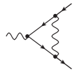
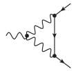
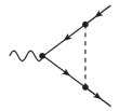
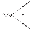
I	II	III	IV
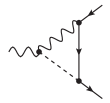
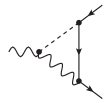
	V	VI
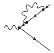
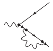
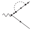
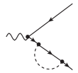
VII	VIII	IX	X

Figure 1: Topologies contributing to two and three-body lepton decays as well as $\gamma,Z\rightarrow\overline{\ell}\ell^{\prime}$.

The contributions from the partner leptons $\tilde{l^{c}}=(\tilde{\nu}^{c}\ \tilde{\ell}^{c})$ only involve topologies III, IV, IX and X in Figure 1 because they do not couple to one T–odd gauge boson and a SM charged lepton at the order considered (see Table 2). Their total contribution is finite as expected and the cancellation of the infinities holds for the contributions exchanging $\tilde{\nu}^{c}$ and $\tilde{\ell}^{c}$ independently in $F_{M}^{\gamma}|_{\tilde{\nu}^{c}}$ and $F_{M}^{\gamma}|_{\tilde{\ell}^{c}}$ respectively. In addition, these contributions decouple from the amplitude in the heavy $\tilde{l}^{c}$ limit. In summary, neglecting $m_{\ell^{\prime}}(\ll m_{\ell})$ and defining $\alpha_{W}=\alpha/s_{W}^{2}$ (with the five terms satisfying $F_{M}^{\gamma}|_{a}=-iF_{E}^{\gamma}|_{a}$),

$$F_{M}^{\gamma} =F_{M}^{\gamma}|_{W_{H}}+F_{M}^{\gamma}|_{A_{H}}+F_{M}^{\gamma}|_{Z_{H}}+F_{M}^{\gamma}|_{\tilde{\nu}^{c}}+F_{M}^{\gamma}|_{\tilde{\ell}^{c}}$$

$$=\sum_{i}V_{\ell^{\prime}i}^{\dagger}V_{i\ell}\ \frac{\alpha_{W}}{16\pi}\frac{m_{\ell}}{M_{W_{H}}^{2}}\left[F^{W}_{M}\left(\frac{m_{\ell_{Hi}}^{2}}{M_{W_{H}}^{2}}\right)+\frac{1}{5}F_{M}^{A/Z}\left(\frac{m_{\ell_{Hi}}^{2}}{M_{A_{H}}^{2}}\right)+F_{M}^{A/Z}\left(\frac{m_{\ell_{Hi}}^{2}}{M_{Z_{H}}^{2}}\right)\right]$$ (12)

$$+\sum_{ijk}V_{\ell^{\prime}i}^{\dagger}\frac{m_{\ell_{Hi}}}{M_{W_{H}}}W_{ij}^{\dagger}W_{jk}\frac{m_{\ell_{Hk}}}{M_{W_{H}}}V_{k\ell}\ \frac{\alpha_{W}}{16\pi}\frac{m_{\ell}}{M_{\Phi}^{2}}\left[F_{M}^{\tilde{\nu}}\left(\frac{m_{\tilde{\nu}^{c}_{j}}^{2}}{M_{\Phi}^{2}}\right)+F_{M}^{\tilde{\ell}}\left(\frac{m_{\tilde{\nu}^{c}_{j}}^{2}}{M_{\Phi}^{2}}\right)\right]\ ,$$

with

$$F^{W}_{M}(x) =\frac{5}{6}-\frac{3x-15x^{2}-6x^{3}}{12(1-x)^{3}}+\frac{3x^{3}}{2(1-x)^{4}}\ln x\ ,$$

$$F_{M}^{A/Z}(x) =-\frac{1}{3}+\frac{2x+5x^{2}-x^{3}}{8(1-x)^{3}}+\frac{3x^{2}}{4(1-x)^{4}}\ln x\,,$$

$$F_{M}^{\tilde{\nu}}(x) =\frac{-1+5x+2x^{2}}{12(1-x)^{3}}+\frac{x^{2}}{2(1-x)^{4}}\ln x\ ,$$ (13)

$$F_{M}^{\tilde{\ell}}(x) =\frac{-4+5x+5x^{2}}{6(1-x)^{3}}-\frac{x(1-2x)}{(1-x)^{4}}\ln x\ .$$

Note that these four loop functions $F_{M}^{W,A/Z,{\tilde{\nu}},{\tilde{\ell}}}$ are finite and depend on the ratio of the particle masses circulating in the loop. Once the global suppression factor $v^{2}/f^{2}$ has been factored out in Eq. (3.1) their own $v^{2}/f^{2}$ corrections can be neglected as they are next order. Thus, in general the (heavy) masses of the different components of the same $SU(2)_{L}$ multiplet can be taken to be degenerate when substituted in $F_{M}^{W,A/Z,{\tilde{\nu}},{\tilde{\ell}}}$ . This is also the case for the components of the scalar electroweak triplet $\Phi$ within $F_{M}^{{\tilde{\nu}},{\tilde{\ell}}}$ and in the denominator multiplying the last line in Eq. (3.1).

$\ell\to\ell^{\prime}\overline{\ell^{\prime}}\ell^{\prime},\ell^{\prime}\overline{\ell^{\prime\prime}}\ell^{\prime\prime},\ell^{\prime}\overline{\ell^{\prime\prime}}\ell^{\prime}$:

These processes involve photon and $Z$ penguin diagrams as well as box contributions which are depicted in Figure 2.

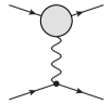
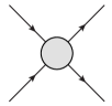
Figure 2: Generic penguin (left) and box (right) amplitudes contributing to three-body $\ell$ decays and to $\mu\rightarrow e$ conversion in nuclei.

$$i\ \Gamma^{\mu}_{\gamma}(p_{\ell},p_{\ell^{\prime}})=i\ e\left\{\left[iF_{M}^{\gamma}(Q^{2})+F_{E}^{\gamma}(Q^{2})\gamma_{5}\right]\sigma^{\mu\nu}Q_{\nu}+F_{L}^{\gamma}(Q^{2})\gamma^{\mu}P_{L}\right\}\ ,$$ (14)

with $Q_{\nu}=(p_{\ell^{\prime}}-p_{\ell})_{\nu}$ and $P_{L,R}=\frac{1}{2}(1\mp\gamma_{5})$. The corresponding right-handed vector form factor vanishes with $m_{\ell^{\prime}}$ and is further suppressed as are the corresponding scalar form factors. The left-handed vector form factor receives contributions from mirror and partner leptons in analogy with the dipole form factors above. Keeping with the notation above,

$$F_{L}^{\gamma} =F_{L}^{\gamma}|_{W_{H}}+F_{L}^{\gamma}|_{A_{H}}+F_{L}^{\gamma}|_{Z_{H}}+F_{L}^{\gamma}|_{\tilde{\nu}^{c}}+F_{L}^{\gamma}|_{\tilde{\ell}^{c}}$$

$$=\sum_{i}V_{\ell^{\prime}i}^{\dagger}V_{i\ell}\ \frac{\alpha_{W}}{4\pi}\frac{Q^{2}}{M_{W_{H}}^{2}}\left[F^{W}_{L}\left(\frac{m_{\ell_{Hi}}^{2}}{M_{W_{H}}^{2}}\right)+\frac{1}{5}F_{L}^{A/Z}\left(\frac{m_{\ell_{Hi}}^{2}}{M_{A_{H}}^{2}}\right)+F_{L}^{A/Z}\left(\frac{m_{\ell_{Hi}}^{2}}{M_{Z_{H}}^{2}}\right)\right]$$ (15)

$$+\sum_{ijk}V_{\ell^{\prime}i}^{\dagger}\frac{m_{\ell_{Hi}}}{M_{W_{H}}}W_{ij}^{\dagger}W_{jk}\frac{m_{\ell_{Hk}}}{M_{W_{H}}}V_{k\ell}\ \frac{\alpha_{W}}{4\pi}\frac{Q^{2}}{M_{\Phi}^{2}}\left[F_{L}^{\tilde{\nu}}\left(\frac{m_{\tilde{\nu}^{c}_{j}}^{2}}{M_{\Phi}^{2}}\right)+F_{L}^{\tilde{\ell}}\left(\frac{m_{\tilde{\nu}^{c}_{j}}^{2}}{M_{\Phi}^{2}}\right)\right]\ ,$$

with the loop functions defined as

$$F^{W}_{L}(x) =-\frac{5}{18}+\frac{12x+x^{2}-7x^{3}}{24(1-x)^{3}}+\frac{12x^{2}-10x^{3}+x^{4}}{12(1-x)^{4}}\ln x\ ,$$

$$F_{L}^{A/Z}(x) =\frac{1}{36}+\frac{18x-11x^{2}-x^{3}}{48(1-x)^{3}}-\frac{4-16x+9x^{2}}{24(1-x)^{4}}\ln x\,,$$

$$F_{L}^{\tilde{\nu}}(x) =\frac{2-7x+11x^{2}}{72(1-x)^{3}}+\frac{x^{3}}{12(1-x)^{4}}\ln x\ ,$$ (16)

$$F_{L}^{\tilde{\ell}}(x) =\frac{20-43x+29x^{2}}{36(1-x)^{3}}+\frac{2-3x+2x^{3}}{6(1-x)^{4}}\ln x\ .$$

The form factor $F_{L}^{\gamma}|_{W_{H}}$ also has a universal infinite contribution which cancels due to the unitarity of the mixing matrices multiplying it. The new contributions proportional to $F_{L}^{\tilde{\nu},\tilde{\ell}}$ decouple when the masses of the partner leptons $\tilde{l}^{c}_{i}$ are taken to infinity. Summarizing, the form factors entering in photon penguin diagrams satisfy $F_{M}^{\gamma}=-iF_{E}^{\gamma}$ while current conservation implies that the vector form factors (in particular, $F_{L}^{\gamma}$) must be proportional to $Q^{2}$ and vanish for on-shell photons. Of course they contribute to photon penguin diagrams which include a photon propagator proportional to $\sim Q^{-2}$.

In contrast, $Z$ penguin diagrams involve the $Z$ boson propagator which for small momentum transfer processes is proportional to $M_{Z}^{-2}$. The dipole form factors, which flip chirality, are proportional to SM lepton masses and negligible when compared to the vector ones while the scalar form factors are also negligible as they are proportional to SM lepton masses. Thus, at leading order the $Z\overline{\ell}\ell^{\prime}$ vertex reduces to,

$$i\ \Gamma^{\mu}_{Z}(p_{\ell},p_{\ell^{\prime}})=i\ e\ F_{L}^{Z}(Q^{2})\gamma^{\mu}P_{L}\ .$$ (17)

The corresponding right-handed vector form factor $F_{R}^{Z}$ is ${\cal O}(m_{\ell}^{2}/f^{2})$ in the LHT and thus negligible at the order we work. As in the case of the photon, the contributions of the T–odd fermions to $F_{L}^{Z}$ result from the running of the mirror and partner leptons inside the loops in Figure 1. Using the Feynman rules introduced above and splitting these contributions as before, we obtain:

$$F_{L}^{Z} =F_{L}^{Z}|_{W_{H}}+F_{L}^{Z}|_{A_{H}}+F_{L}^{Z}|_{Z_{H}}+F_{L}^{Z}|_{\tilde{\nu}^{c}}+F_{L}^{Z}|_{\tilde{\ell}^{c}}$$

$$=\sum_{i}V_{\ell^{\prime}i}^{\dagger}V_{i\ell}\ \frac{\alpha_{W}}{8\pi s_{W}c_{W}}\left\{\frac{v^{2}}{8f^{2}}H^{W(0)}_{L}\left(\frac{m_{\ell_{Hi}}^{2}}{M_{W_{H}}^{2}}\right)+\frac{Q^{2}}{M_{W_{H}}^{2}}H_{L}^{W}\left(\frac{m_{\ell_{Hi}}^{2}}{M_{W_{H}}^{2}}\right)\right.$$ (18)

$$\quad\quad\quad\quad\quad\quad\quad\quad\quad\quad\left.+(1-2c_{W}^{2})\frac{Q^{2}}{M_{W_{H}}^{2}}\left[\frac{1}{5}H_{L}^{A/Z}\left(\frac{m_{\ell_{Hi}}^{2}}{M_{A_{H}}^{2}}\right)+H_{L}^{A/Z}\left(\frac{m_{\ell_{Hi}}^{2}}{M_{Z_{H}}^{2}}\right)\right]\right\}$$

$$+\sum_{ijk}V_{\ell^{\prime}i}^{\dagger}\frac{m_{\ell_{Hi}}}{M_{W_{H}}}W_{ij}^{\dagger}W_{jk}\frac{m_{\ell_{Hk}}}{M_{W_{H}}}V_{k\ell}\ \frac{\alpha_{W}}{8\pi s_{W}c_{W}}\frac{Q^{2}}{M_{\Phi}^{2}}\left[H_{L}^{\tilde{\nu}}\left(\frac{m_{\tilde{\nu}^{c}_{j}}^{2}}{M_{\Phi}^{2}}\right)+(1-2c_{W}^{2})H_{L}^{\tilde{\ell}}\left(\frac{m_{\tilde{\nu}^{c}_{j}}^{2}}{M_{\Phi}^{2}}\right)\right]\ ,$$

with the loop functions defined

$$H^{W(0)}_{L}(x) =\frac{6x-x^{2}}{1-x}+\frac{2x+3x^{2}}{(1-x)^{2}}\ln x\ ,$$

$$H^{W}_{L}(x) =2F_{L}^{A/Z}(x)-2c_{W}^{2}F_{L}^{W}\ ,$$

$$H_{L}^{A/Z}(x) =F_{L}^{A/Z}(x)\ ,$$ (19)

$$H_{L}^{\tilde{\nu}}(x) =\frac{1}{2}F_{L}^{\tilde{\ell}}(x)-2c_{W}^{2}F_{L}^{\tilde{\nu}}(x)\ ,$$

$$H_{L}^{\tilde{\ell}}(x) =F_{L}^{\tilde{\ell}}(x)\ .$$

Again $F_{L}^{Z}|_{W_{H}}$ has a universal infinite loop contribution which cancels due to the unitarity of the mixing matrices and there are similar relations among the finite loop functions $F_{L}^{W,A/Z,{\tilde{\nu}},{\tilde{\ell}}}$ and $H_{L}^{W,A/Z,{\tilde{\nu}},{\tilde{\ell}}}$ for the photon and left-handed $Z$ vector form factors in Eqs. (3.1) and (3.1). The form factor $F_{L}^{Z}|_{W_{H}}$ has two different finite contributions, one which is proportional to $H^{W(0)}_{L}$ and independent of $Q^{2}$, so absent in the photon case, and another linear in $Q^{2}$ and proportional to $H^{W}_{L}$ (second line in Eq. (3.1)). Only the first contributes to three-body lepton decays and to $\mu\to e$ conversion in nuclei. The second one as well as all the other contributions which are proportional to $Q^{2}$ in $F_{L}^{Z}$ (see Eq. (3.1)) are negligible as long as $Q^{2}\ll v^{2}$. We give the complete result here because we will make use of it when discussing leptonic on-shell $Z$ decays below where we also provide further details of the calculation.

The $\ell(p_{\ell})\to\ell^{\prime}(p_{1})\overline{\ell^{\prime}}(p_{2})\ell^{\prime}(p_{3})$ amplitude ${\cal M}^{\ell\to\ell^{\prime}_{1}\overline{\ell^{\prime}}_{2}\ell^{\prime}_{3}}$ then gets contributions from the photon and $Z$ vertices in Eqs. (14) and (17) after contracting them with the corresponding gauge boson propagators and the tree-level SM leptonic vertices. It also receives contributions from the box diagrams shown in Figure 3.

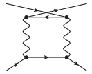
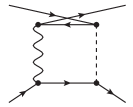
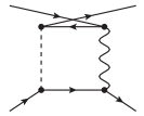
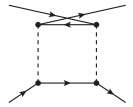
A1	A2	A3	A4
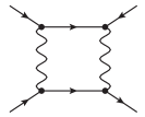
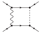
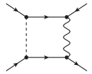
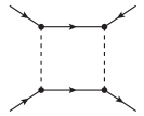
B1	B2	B3	B4

Figure 3: Box diagram topologies contributing to three-body $\ell$ decays and to $\mu\rightarrow e$ conversion in nuclei. Crossed diagrams with the two outgoing leptons (whether they are identical or not) exchanged must be added in the three-body leptonic $\ell$ decays.

Following the analysis in delAguila:2008zu (see also Hisano:1995cp ; Arganda:2005ji ) we write the full $\ell\to\ell^{\prime}_{1}{\overline{\ell^{\prime}}}_{2}\ell^{\prime}_{3}$ amplitude as,

$${\cal M}^{\ell\to\ell^{\prime}_{1}{\overline{\ell^{\prime}_{2}}}\ell^{\prime}_{3}}={\cal M}^{\ell\to\ell^{\prime}_{1}{\overline{\ell^{\prime}_{2}}}\ell^{\prime}_{3}}_{\gamma}+{\cal M}^{\ell\to\ell^{\prime}_{1}{\overline{\ell^{\prime}_{2}}}\ell^{\prime}_{3}}_{Z}+{\cal M}^{\ell\to\ell^{\prime}_{1}{\overline{\ell^{\prime}_{2}}}\ell^{\prime}_{3}}_{\rm Box}\ ,$$ (20)

where we have defined the individual amplitudes as,

$${\cal M}^{\ell\to\ell^{\prime}_{1}{\overline{\ell^{\prime}_{2}}}\ell^{\prime}_{3}}_{\gamma}= \,\overline{u}(p_{1})\,e\left[i\,F_{M}^{\gamma}(0)\,2P_{R}\,\sigma^{\mu\nu}(p_{1}-p_{\ell})_{\nu}+F_{L}^{\gamma}((p_{1}-p_{\ell})^{2})\gamma^{\mu}P_{L}\right]u(p_{\ell})$$

$$\times\frac{1}{(p_{1}-p_{\ell})^{2}}\overline{u}(p_{3})\gamma_{\mu}e\,v(p_{2})-\left(p_{1}\leftrightarrow p_{3}\right)\ ,$$ (21)

$${\cal M}^{\ell\to\ell^{\prime}_{1}{\overline{\ell^{\prime}_{2}}}\ell^{\prime}_{3}}_{Z}= \,\overline{u}(p_{1})\,(-eF_{L}^{Z}(0))\,\gamma^{\mu}P_{L}u(p_{\ell})\frac{1}{M_{Z}^{2}}\overline{u}(p_{3})\gamma_{\mu}\,(g_{L}^{Z}P_{L}+g_{R}^{Z}P_{R})\,v(p_{2})$$

$$\,-\left(p_{1}\leftrightarrow p_{3}\right)\ ,$$ (22)

$${\cal M}^{\ell\to\ell^{\prime}_{1}{\overline{\ell^{\prime}_{2}}}\ell^{\prime}_{3}}_{\rm Box}= \,e^{2}B_{L}(0)\ \overline{u}(p_{1})\,\gamma^{\mu}P_{L}u(p_{\ell})\ \overline{u}(p_{3})\gamma_{\mu}P_{L}\,v(p_{2})\ ,$$ (23)

with $F_{E}^{\gamma}=i\,F_{M}^{\gamma}$. The photon magnetic and $Z$ left-handed vector form factors, $F_{M}^{\gamma}(0)$ and $F_{L}^{Z}(0)$ respectively, are evaluated at $Q^{2}=(p_{1}-p_{\ell})^{2}=0$ because their leading terms are momentum independent for small momentum transfer $Q^{2}\sim m_{\ell}^{2}$ while the photon left-handed vector form factor, $F_{L}^{\gamma}((p_{1}-p_{\ell})^{2})$, is linear in $Q^{2}$. The $g_{L}^{Z}$ and $g_{R}^{Z}$ couplings of the $Z$ boson to charged leptons are given in Table 2.

Moving on to the box diagrams shown in Figure 3, these all reduce to the same product of currents in Eq. (23) in the limit of zero external momenta delAguila:2008zu (all internal masses are much larger than the external ones). The box loop-integrals are finite by power counting and in this limit their contributions can all be absorbed into the form factor $e^{2}\,B_{L}(0)$. In addition to the contributions from mirror leptons accounted for in delAguila:2008zu , those from partner leptons must also be included. Bearing in mind the degenerate mass limit for different components of the heavy T–odd $SU(2)_{L}$ multiplets we can group them according to the bosonic particle masses running in the loop,

$$B_{L}(0)=B_{L}^{W_{H}W_{H}+Z_{H}Z_{H}}+B_{L}^{A_{H}A_{H}}+B_{L}^{A_{H}Z_{H}}+B_{L}^{\Phi\Phi}\ ,$$ (24)

where we have defined the functions,

$$B_{L}^{W_{H}W_{H}+Z_{H}Z_{H}} =\frac{\alpha_{W}}{32\pi s_{W}^{2}}\frac{1}{M_{W_{H}}^{2}}\times$$

$$\sum_{ij}\chi^{\ell\ell^{\prime}\ell^{\prime}\ell^{\prime}}_{ij} \left[\frac{1}{2}\left(1+\frac{m_{\ell_{Hi}}^{2}}{M_{W_{H}}^{2}}\frac{m_{\ell_{Hj}}^{2}}{M_{W_{H}}^{2}}\right)\tilde{d}\left(\frac{m_{\ell_{Hi}}^{2}}{M_{W_{H}}^{2}},\frac{m_{\ell_{Hj}}^{2}}{M_{W_{H}}^{2}}\right)-4\frac{m_{\ell_{Hi}}^{2}}{M_{W_{H}}^{2}}\frac{m_{\ell_{Hj}}^{2}}{M_{W_{H}}^{2}}d\left(\frac{m_{\ell_{Hi}}^{2}}{M_{W_{H}}^{2}},\frac{m_{\ell_{Hj}}^{2}}{M_{W_{H}}^{2}}\right)\right]\ ,$$

$$B_{L}^{A_{H}A_{H}} =\frac{\alpha_{W}}{32\pi s_{W}^{2}}\frac{1}{M_{W_{H}}^{2}}\sum_{ij}\chi^{\ell\ell^{\prime}\ell^{\prime}\ell^{\prime}}_{ij}\left[-\frac{3}{50}\frac{M_{A_{H}}^{2}}{M_{W_{H}}^{2}}\tilde{d}\left(\frac{m_{\ell_{Hi}}^{2}}{M_{A_{H}}^{2}},\frac{m_{\ell_{Hj}}^{2}}{M_{A_{H}}^{2}}\right)\right]\ ,$$ (25)

$$B_{L}^{A_{H}Z_{H}} =\frac{\alpha_{W}}{32\pi s_{W}^{2}}\frac{1}{M_{W_{H}}^{2}}\sum_{ij}\chi^{\ell\ell^{\prime}\ell^{\prime}\ell^{\prime}}_{ij}\left[-\frac{3}{5}{\tilde{d}}^{\prime}\left(\frac{m_{\ell_{Hi}}^{2}}{M_{A_{H}}^{2}},\frac{m_{\ell_{Hj}}^{2}}{M_{A_{H}}^{2}},\frac{M_{W_{H}}^{2}}{M_{A_{H}}^{2}}\right)\right]\ ,$$

$$B_{L}^{\Phi\Phi} =\frac{\alpha_{W}}{32\pi s_{W}^{2}}\frac{1}{M_{\Phi}^{2}}\sum_{ij}\tilde{\chi}^{\ell\ell^{\prime}\ell^{\prime}\ell^{\prime}}_{ij}\tilde{d}\left(\frac{m_{{\tilde{\nu}}^{c}_{i}}^{2}}{M_{\Phi}^{2}},\frac{m_{{\tilde{\nu}}^{c}_{j}}^{2}}{M_{\Phi}^{2}}\right)\ .$$

The mixing coefficients are defined in Eqs. (3) and (4) with $\ell^{\prime\prime\prime}=\ell^{\prime\prime}=\ell^{\prime}$ respectively while the loop functions read,

$${\tilde{d}}(x,y) =\frac{x^{2}\ln x}{(1-x)^{2}(y-x)}+\frac{y^{2}\ln y}{(1-y)^{2}(x-y)}-\frac{1}{(1-x)(1-y)}\ ,$$

$$d(x,y) =\frac{x\ln x}{(1-x)^{2}(y-x)}+\frac{y\ln y}{(1-y)^{2}(x-y)}-\frac{1}{(1-x)(1-y)}\ ,$$ (26)

$${\tilde{d}}^{\prime}(x,y,z) =\frac{x^{2}\ln x}{(1-x)(y-x)(z-x)}+\frac{y^{2}\ln y}{(1-y)(x-y)(z-y)}+\frac{z^{2}\ln z}{(1-z)(x-z)(y-z)}\ ,$$

with ${\tilde{d}}(x,y)={\tilde{d}}^{\prime}(x,y,1)$. The new contributions from the partner leptons ${\tilde{\nu}}^{c}$ and ${\tilde{\ell}}^{c}$ are equal (neglecting small mass differences within the scalar triplet $\Phi$ components) and included in $B_{L}^{\Phi\Phi}$. After integrating the three-body phase space the decay width reads:

$$\Gamma(\ell\to\ell^{\prime}\overline{\ell^{\prime}}\ell^{\prime}) =\frac{\alpha^{2}m_{\ell}^{5}}{96\pi}\Big{\{}3|A_{L}|^{2}+2|A_{R}|^{2}\left(8\ln\frac{m_{\ell}}{m_{\ell^{\prime}}}-13\right)+2|F_{LL}|^{2}+|F_{LR}|^{2}+\frac{1}{2}|B_{L}|^{2}$$

$$-\left[6A_{L}A_{R}^{*}-(A_{L}-2A_{R})(2F_{LL}^{*}+F_{LR}^{*}+B_{L}^{*})-F_{LL}B_{L}^{*}+\mbox{h.c.}\right]\Big{\}}\ ,$$ (27)

where we have defined in order to simplify the expression:

$$A_{L}=\frac{F_{L}^{\gamma}}{Q^{2}},\ A_{R}=\frac{2F_{M}^{\gamma}(0)}{m_{\ell}},\ F_{LL}=-\frac{g_{L}F_{L}^{Z}(0)}{eM_{Z}^{2}},\ F_{LR}=-\frac{g_{R}F_{L}^{Z}(0)}{eM_{Z}^{2}},\ B_{L}=B_{L}(0),\,$$ (28)

with $g_{L,R}$ the corresponding $Z$ couplings to the charged lepton $\ell^{\prime}$ (see Table 2). With these results for $\ell\to\ell^{\prime}\overline{\ell^{\prime}}\ell^{\prime}$, the other LFV three-body lepton decays are easily obtained.

For the $\ell(p_{\ell})\to\ell^{\prime}(p_{1})\overline{\ell^{\prime\prime}}(p_{2})\ell^{\prime\prime}(p_{3})$ amplitude there are no crossed penguin diagram contributions due to swapping $\ell^{\prime}$ and $\ell^{\prime\prime}$ because two gauge boson LFV transitions would be needed. This implies a higher order process both in loops and in $v^{2}/f^{2}$. This means that the $\ell(p_{\ell})\to\ell^{\prime}(p_{1})\overline{\ell^{\prime\prime}}(p_{2})\ell^{\prime\prime}(p_{3})$ amplitude ${\cal M}^{\ell\to\ell^{\prime}_{1}\overline{\ell^{\prime\prime}}_{2}\ell^{\prime\prime}_{3}}$ has no $p_{1}\leftrightarrow p_{3}$ term in Eqs. (3.1) and (3.1). However, for the box amplitudes there are additional diagrams at this order for swapping $\ell^{\prime}$ and $\ell^{\prime\prime}$. These are automatically taken into account by the mixing coefficient definitions in Eqs. (3) and (4) once the flavor factors with $\ell\ell^{\prime}\ell^{\prime}\ell^{\prime}$ are replaced by the appropriate ones with $\ell\ell^{\prime}\ell^{\prime\prime}\ell^{\prime\prime}$. Furthermore, now there is no symmetry factor of 1/2 in the phase space integration needed to obtain the decay width because all three final leptons are distinguishable. The final decay width can be written as (see footnote 18),

$$\Gamma(\ell\to\ell^{\prime}\overline{\ell^{\prime\prime}}\ell^{\prime\prime}) =\frac{\alpha^{2}m_{\ell}^{5}}{96\pi}\Big{\{}2|A_{L}|^{2}+4|A_{R}|^{2}\left(4\ln\frac{m_{\ell}}{m_{\ell^{\prime\prime}}}-7\right)+|F_{LL}|^{2}+|F_{LR}|^{2}+\left|B_{L}\right|^{2}$$

$$-\left[4A_{L}A_{R}^{*}-(A_{L}-2A_{R})\left(F_{LL}^{*}+F_{LR}^{*}+\frac{B_{L}^{*}}{2}\right)-F_{LL}\frac{B_{L}^{*}}{2}+\mbox{h.c.}\right]\Big{\}}\,,$$ (29)

with the same simplifying definitions as in Eq. (28) and corresponding changes to account for the $Z$ couplings to the charged lepton $\ell^{\prime\prime}$.

Finally, for the double flavor violating decay $\ell(p_{\ell})\to\ell^{\prime}(p_{1})\overline{\ell^{\prime\prime}}(p_{2})\ell^{\prime}(p_{3})$ the amplitude ${\cal M}^{\ell\to\ell^{\prime}_{1}\overline{\ell^{\prime\prime}_{2}}\ell^{\prime}_{3}}$ has no penguin contributions at the order we consider (see footnote 8). The box contributions on the other hand are the same as for $\ell(p_{\ell})\to\ell^{\prime}(p_{1})\overline{\ell^{\prime}}(p_{2})\ell^{\prime}(p_{3})$ but replacing the corresponding flavor coefficients in Eq. (3.1) with those in this decay $\ell\ell^{\prime}\ell^{\prime\prime}\ell^{\prime}$. The decay width is also the same as in Eq. (3.1) but with the box loop form factor $|B_{L}|^{2}$ term only. This gives for the total decay width (with same phase space as for $\ell\to\ell^{\prime}\overline{\ell^{\prime}}\ell^{\prime}$),

$$\Gamma(\ell\to\ell^{\prime}\overline{\ell^{\prime\prime}}\ell^{\prime})=\frac{\alpha^{2}m_{\ell}^{5}}{192\,\pi}\left|B_{L}\right|^{2}\,.$$ (30)

$\mu\ {\rm N}\rightarrow e\ {\rm N}$:

For this transition we follow Ref. delAguila:2010nv where the contributions of the (T–odd) mirror fermions to $\mu\rightarrow e$ conversion in nuclei are discussed. This process has penguin and box contributions as in Figure 2. As for the leptonic decay $\ell\to\ell^{\prime}\overline{\ell^{\prime\prime}}\ell^{\prime\prime}$, it has no crossed penguin diagrams because the lower fermionic line where the gauge boson is attached is now a coherent sum of quarks composing the probed nucleus. There is also no crossed box contributions due to the exchange of leptons. Putting everything together, including the new partner fermion contributions, we can write the $\mu\to e$ conversion through the interaction with a quark $q$ equal to $u$ or $d$:

$${\cal M}^{\mu q\rightarrow eq}={\cal M}^{\mu q\rightarrow eq}_{\gamma}+{\cal M}^{\mu q\rightarrow eq}_{Z}+{\cal M}^{\mu q\rightarrow eq}_{\rm Box}\ ,$$ (31)

with the amplitudes defined as,

$${\cal M}^{\mu q\rightarrow eq}_{\gamma}= \,\overline{u}(p_{1})\,e\left[i\,F_{M}^{\gamma}(0)\,2P_{R}\,\sigma^{\mu\nu}(p_{1}-p_{\ell})_{\nu}+F_{L}^{\gamma}((p_{1}-p_{\ell})^{2})\gamma^{\mu}P_{L}\right]u(p_{\ell})$$

$$\times\frac{1}{(p_{1}-p_{\ell})^{2}}\overline{u}(p_{3})\gamma_{\mu}\,(g_{Lq}^{\gamma}P_{L}+g_{Rq}^{\gamma}P_{R})\,v(p_{2})\ ,$$ (32)

$${\cal M}^{\mu q\rightarrow eq}_{Z}= \,\overline{u}(p_{1})\,(-eF_{L}^{Z}(0))\,\gamma^{\mu}P_{L}u(p_{\ell})\frac{1}{M_{Z}^{2}}\overline{u}(p_{3})\gamma_{\mu}\,(g_{Lq}^{Z}P_{L}+g_{Rq}^{Z}P_{R})\,v(p_{2})\ ,$$ (33)

$${\cal M}^{\mu q\rightarrow eq}_{\rm Box}= \,e^{2}B_{L}^{q}(0)\ \overline{u}(p_{1})\,\gamma^{\mu}P_{L}u(p_{\ell})\ \overline{u}(p_{3})\gamma_{\mu}P_{L}\,v(p_{2})\ .$$ (34)

The form factors $F_{M}^{\gamma}(0)$, $F_{L}^{\gamma}$, and $F_{L}^{Z}(0)$ are given in Eqs. (3.1), (3.1), and (3.1) respectively while the couplings $g_{L(R)q}^{\gamma(Z)}$ are gathered in Table 5 for $q=u,d$. The three form factors include the contributions from both mirror and partner leptons, the latter of which have not been previously computed. Analogously, $B_{L}^{q}(0)$ can be read from Eqs. (24) and (3.1) and replacing the appropriate charges, masses, and mixings (and multiplying by a global factor of one-half to account for no crossed box diagrams for swapping leptons). The mirror fermion contribution is detailed in Ref. delAguila:2010nv , and is contained in the corresponding sums exchanging $W_{H}W_{H}$ (first two terms), $Z_{H}Z_{H}$ (third term), $A_{H}A_{H}$ (fourth term), and $A_{H}Z_{H}$ (fifth term) in Eq. (3.1):

$$B_{Lu}^{W_{H}W_{H}+Z_{H}Z_{H}+A_{H}A_{H}+A_{H}Z_{H}} =\frac{\alpha_{W}}{32\pi s_{W}^{2}}\frac{1}{M_{W_{H}}^{2}}\times$$

$$\sum_{ij}\chi_{ij}^{u}\left[-\left(8+\frac{1}{2}\frac{m_{\ell_{Hi}}^{2}}{M_{W_{H}}^{2}}\right.\right. \left.\frac{m_{d_{Hj}}^{2}}{M_{W_{H}}^{2}}\right)\tilde{d}\left(\frac{m_{\ell_{Hi}}^{2}}{M_{W_{H}}^{2}},\frac{m_{d_{Hj}}^{2}}{M_{W_{H}}^{2}}\right)+4\frac{m_{\ell_{Hi}}^{2}}{M_{W_{H}}^{2}}\frac{m_{d_{Hj}}^{2}}{M_{W_{H}}^{2}}d\left(\frac{m_{\ell_{Hi}}^{2}}{M_{W_{H}}^{2}},\frac{m_{d_{Hj}}^{2}}{M_{W_{H}}^{2}}\right)$$

$$-\frac{3}{2}\tilde{d}\left(\frac{m_{\ell_{Hi}}^{2}}{M_{W_{H}}^{2}},\frac{m_{d_{Hj}}^{2}}{M_{W_{H}}^{2}}\right) \left.-\frac{3}{50}\frac{M_{A_{H}}^{2}}{M_{W_{H}}^{2}}\tilde{d}\left(\frac{m_{\ell_{Hi}}^{2}}{M_{A_{H}}^{2}},\frac{m_{d_{Hj}}^{2}}{M_{A_{H}}^{2}}\right)+\frac{3}{5}\tilde{d}^{\prime}\left(\frac{m_{\ell_{Hi}}^{2}}{M_{A_{H}}^{2}},\frac{m_{d_{Hj}}^{2}}{M_{A_{H}}^{2}},\frac{M_{W_{H}}^{2}}{M_{A_{H}}^{2}}\right)\right]\,,$$

$$B_{Ld}^{W_{H}W_{H}+Z_{H}Z_{H}+A_{H}A_{H}+A_{H}Z_{H}} =\frac{\alpha_{W}}{32\pi s_{W}^{2}}\frac{1}{M_{W_{H}}^{2}}\times$$ (35)

$$\sum_{ij}\chi_{ij}^{d}\left[\left(2+\frac{1}{2}\frac{m_{\ell_{Hi}}^{2}}{M_{W_{H}}^{2}}\right.\right. \left.\frac{m_{d_{Hj}}^{2}}{M_{W_{H}}^{2}}\right)\tilde{d}\left(\frac{m_{\ell_{Hi}}^{2}}{M_{W_{H}}^{2}},\frac{m_{d_{Hj}}^{2}}{M_{W_{H}}^{2}}\right)-4\frac{m_{\ell_{Hi}}^{2}}{M_{W_{H}}^{2}}\frac{m_{d_{Hj}}^{2}}{M_{W_{H}}^{2}}d\left(\frac{m_{\ell_{Hi}}^{2}}{M_{W_{H}}^{2}},\frac{m_{d_{Hj}}^{2}}{M_{W_{H}}^{2}}\right)$$

$$-\frac{3}{2}\tilde{d}\left(\frac{m_{\ell_{Hi}}^{2}}{M_{W_{H}}^{2}},\frac{m_{d_{Hj}}^{2}}{M_{W_{H}}^{2}}\right) \left.-\frac{3}{50}\frac{M_{A_{H}}^{2}}{M_{W_{H}}^{2}}\tilde{d}\left(\frac{m_{\ell_{Hi}}^{2}}{M_{A_{H}}^{2}},\frac{m_{d_{Hj}}^{2}}{M_{A_{H}}^{2}}\right)-\frac{3}{5}\tilde{d}^{\prime}\left(\frac{m_{\ell_{Hi}}^{2}}{M_{A_{H}}^{2}},\frac{m_{d_{Hj}}^{2}}{M_{A_{H}}^{2}},\frac{M_{W_{H}}^{2}}{M_{A_{H}}^{2}}\right)\right]\,.$$

Obviously, now the mixing coefficients involve mirror lepton mixing matrices as well as mirror quark ones, defined in Eq. (9):

$$\chi_{ij}^{u}=V_{ei}^{\dagger}V_{i\mu}V_{uj}^{u\dagger}V_{ju}^{u}\,,\quad\chi_{ij}^{d}=V_{ei}^{\dagger}V_{i\mu}V_{dj}^{d\dagger}V_{jd}^{d}\,.$$ (36)

The (new) partner fermion contribution can be also read from Eq. (3.1). In this case the exchanged bosons are the charged scalar triplet components with the contributions from the different field sets running in the box being equal up to mixing coefficients $\tilde{\chi}^{u,d}_{ij}$:

$$B_{Lu}^{\Phi\Phi} =\frac{\alpha_{W}}{64\pi s_{W}^{2}}\frac{1}{M_{\Phi}^{2}}\sum_{ij}\tilde{\chi}^{u}_{ij}\tilde{d}\left(\frac{m^{2}_{\tilde{\nu}^{c}_{i}}}{M_{\Phi}^{2}},\frac{m^{2}_{\tilde{u}_{j}}}{M_{\Phi}^{2}}\right)\,,$$

$$B_{Ld}^{\Phi\Phi} =5\frac{\alpha_{W}}{64\pi s_{W}^{2}}\frac{1}{M_{\Phi}^{2}}\sum_{ij}\tilde{\chi}^{d}_{ij}\tilde{d}\left(\frac{m^{2}_{\tilde{\nu}^{c}_{i}}}{M_{\Phi}^{2}},\frac{m^{2}_{\tilde{u}_{j}}}{M_{\Phi}^{2}}\right)\,,$$ (37)

where the mixing coefficients are defined in terms of the mixing matrices as,

$$\tilde{\chi}^{u}_{ij}=\sum_{k,n,r,s}V_{ek}^{\dagger}\frac{m_{\ell_{Hk}}}{M_{W_{H}}}W_{ki}^{\dagger}W_{in}\frac{m_{\ell_{Hn}}}{M_{W_{H}}}V_{n\mu}V^{u\dagger}_{ur}\frac{m_{d_{Hr}}}{M_{W_{H}}}W_{rj}^{q\dagger}W_{js}^{q}\frac{m_{d_{Hs}}}{M_{W_{H}}}V^{u}_{su}\,,$$

$$\tilde{\chi}^{d}_{ij}=\sum_{k,n,r,s}V_{ek}^{\dagger}\frac{m_{\ell_{Hk}}}{M_{W_{H}}}W_{ki}^{\dagger}W_{in}\frac{m_{\ell_{Hn}}}{M_{W_{H}}}V_{n\mu}V^{d\dagger}_{dr}\frac{m_{d_{Hr}}}{M_{W_{H}}}W_{rj}^{q\dagger}W_{js}^{q}\frac{m_{d_{Hs}}}{M_{W_{H}}}V^{d}_{sd}\,.$$ (38)

The extra factor of 5 for $B_{Ld}^{\Phi\Phi}$ accounts for the fact that for down quarks we can have $\tilde{x}$ (of charge 5/3) and $\Phi^{++}$ as well as $\tilde{u}$ (of charge 2/3) and $\Phi^{+}$ circulating in the loop and keeping in mind the components of the heavy $SU(2)_{L}$ multiplets are degenerate at the order we work. Summing the different box contributions,

$$B_{L}^{q}(0)=B_{Lq}^{W_{H}W_{H}+Z_{H}Z_{H}+A_{H}A_{H}+A_{H}Z_{H}}+B_{Lq}^{\Phi\Phi}\,,\quad q=u,d\,.$$ (39)

This gives for the corresponding conversion width in a nucleus N with $Z$ protons and $N$ neutrons Hisano:1995cp (with $Z$ not to be confused with the $Z$ gauge boson),

$$\Gamma(\mu\ {\rm N}\to e\ {\rm N})= \ \alpha^{5}\frac{Z^{4}_{\rm eff}}{Z}F_{p}^{2}m_{\mu}^{5}\left|2Z(A_{L}+A_{R})-(2Z+N)(F_{LL}^{u}+F_{LR}^{u}+B_{L}^{u})\right.$$

$$\left.-\ (Z+2N)(F_{LL}^{d}+F_{LR}^{d}+B_{L}^{d})\right|^{2}\ ,$$ (40)

where $Z_{\rm eff}$ is the nucleus effective charge for the muon and $F_{p}$ the associated form factor. We also have $m_{\ell}=m_{\mu}$ in the definition of $A_{R}$ in Eq. (28) while $g_{L(R)q}^{Z}$ are the $Z$ couplings to the quark $q=u,d$ given in Table 5 and entering in the definition of $F_{LL(LR)}^{q}$ of the same equation.

Nucleus	$N$	$Z$	$Z_{\rm eff}$	$F_{p}$	$\Gamma_{\rm capture}[{\rm GeV}]$
${}^{27}_{13}{\rm Al}$	14	13	11.5	0.64	$4.6\times 10^{-19}$
${}^{48}_{22}{\rm Ti}$	26	22	17.6	0.54	$1.7\times 10^{-18}$
${}^{197}_{\ 79}{\rm Au}$	118	79	33.5	0.16	$8.6\times 10^{-18}$

Table 7: Input parameters for the nuclei considered in our analysis (see Refs. Kitano:2002mt and Suzuki:1987jf ).

In Table 7 we gather the input parameters for Al and for Ti and Au, to be used below when comparing with future Abusalma:2018xem ; Angelique:2018svf and current limits, respectively.

3.2 One-loop contributions to $Z\to\overline{\ell}\ell^{\prime}$ decays

Let us finally evaluate the $Z$ boson decay into a pair of charged leptons of different flavor. The corresponding $Z$ penguin contributing to rare processes with small transfer momentum $Q^{2}\sim m_{\ell}^{2}$ has been discussed in the previous subsection (see Eqs. (17), (3.1) and (3.1)). In that case only the first contribution to $F_{L}^{Z}$ in Eq. (3.1), proportional to $v^{2}/f^{2}$, is relevant because $Q^{2}\ll v^{2}$. However, in $Z$ decays with $Q^{2}=M_{Z}^{2}\sim v^{2}$ all the contributions to $F_{L}^{Z}$ in Eq. (3.1) are comparable and must be taken into account. Overall the $Z\overline{\ell}\ell^{\prime}$ vertex only receives significant contributions from the $F_{L}^{Z}$ form factor (see Eq. (17)), as all others are suppressed by (light) SM lepton masses. Therefore, the corresponding amplitude for a $Z$ boson with polarization $s$ decaying into $\overline{\ell}\ell^{\prime}$ can be written in our case

$${{\cal M}_{s}}(Z\rightarrow\overline{\ell}\ell^{\prime})=i\,e\ \bar{u}(p_{\ell^{\prime}},m_{\ell^{\prime}})\ F^{Z}_{L}(M_{Z}^{2})\ \gamma_{\mu}P_{L}\ v(p_{\ell},m_{\ell})\ \epsilon_{s}^{\mu}(p_{\ell^{\prime}}-p_{\ell})\ ,$$ (41)

where $\epsilon_{s}^{\mu}(p_{\ell^{\prime}}-p_{\ell})$ is the $Z$ polarization vector, with $Q=p_{\ell^{\prime}}-p_{\ell}$ and $Q^{2}=M_{Z}^{2}$. Hence, the $Z$ width reduces to

$$\Gamma(Z\rightarrow\overline{\ell}\ell^{\prime})=\frac{\alpha}{3}M_{Z}|F^{Z}_{L}(M_{Z}^{2})|^{2}\ .$$ (42)

In order to conclude this section we provide further details of the calculation of $F_{L}^{Z}$ in Eqs. (3.1) and (3.1) where we obtained the leading contributions from the full T–odd spectrum in the LHT. It is instructive to explicitly check the cancellation of the divergent terms in order to compare with the corresponding Higgs decay and previous calculations of LFV $Z$ decays which did not include the partner leptons and electroweak triplet $\Phi$. The unitarity of the mixing matrices $V$ and $W$ ensures that one is left only with divergent terms for a given topology (see Figure 1) and T–odd fields running in the loop which have at least two $m_{\ell_{Hi}}$ insertions (see Eq. (3.1)). These terms can be ${\cal O}(1)$ or ${\cal O}(\frac{v^{2}}{f^{2}})$, but in both cases must sum to zero. This can be ensured for the ${\cal O}(1)$ terms because they are generated by dimension four operators which can always be assumed (rotated) to be flavor diagonal. For the higher dimensional operators this is not the case and a more subtle cancellation between different divergences is needed.

These cancellations can be seen explicitly in Tables 8 and 9.

$C_{\rm UV}^{(1)}\$	I	II	III	IV	V+VI	VII+VIII	IX+X	Sum
$W_{H},\nu_{H}\$	0	0	$-$	$-$	$-$	$0$	$-$	$0$
$W_{H},\omega,\nu_{H}\$	$-$	$-$	$-$	$-$	$0$	$-$	$-$	$0$
$\omega,\nu_{H}\$	$-$	$-$	$\frac{1}{2}$	$-1+s_{W}^{2}$	$-$	$-$	$\frac{1}{2}-s_{W}^{2}$	$\bullet$
$A_{H},\ell_{H}\$	0	$\bullet$	$-$	$-$	$-$	0	$-$	$\bullet$
$\eta,\ell_{H}\$	$-$	$-$	$-\frac{1}{20}+\frac{s^{2}_{W}}{10}$	$\bullet$	–	$-$	$\frac{1}{20}-\frac{s^{2}_{W}}{10}$	$\bullet$
$Z_{H},\ell_{H}\$	0	$\bullet$	$-$	$-$	$-$	0	$-$	$\bullet$
$\omega,\ell_{H}\$	$-$	$-$	$-\frac{1}{4}+\frac{s^{2}_{W}}{2}$	$\bullet$	–	–	$\frac{1}{4}-\frac{s^{2}_{W}}{2}$	$\bullet$
$\Phi,\tilde{\nu}^{c}\$	–	–	$-\frac{1}{2}$	$s_{W}^{2}$	–	–	$\frac{1}{2}-s_{W}^{2}$	$\bullet$
$\Phi,\tilde{\ell}^{c}\$	–	–	$1-2s_{W}^{2}$	$-2+4s_{W}^{2}$	–	–	$1-2s_{W}^{2}$	$\bullet$
Total	0	0	$\frac{7}{10}-\frac{7s_{W}^{2}}{5}$	$-3+6s_{W}^{2}$	$0$	0	$\frac{23}{10}-\frac{23s_{W}^{2}}{5}$	$\bullet$

Table 8: The ${\cal O}(1)$ divergent contributions proportional to $\frac{1}{\epsilon}$ ($\epsilon=4-d$) of each particle set running in the loop and topology shown in Figure 1. A dash means that the field set does not run in the diagram whereas a bullet indicates the infinite and finite parts vanish.

$C_{\rm UV}^{(\frac{v^{2}}{f^{2}})}$	I	II	III	IV	V+VI	VII+VIII	IX+X	Sum
$W_{H},\nu_{H}$	0	0	$-$	$-$	$-$	$0$	$-$	$0$
$W_{H},\omega,\nu_{H}$	$-$	$-$	$-$	$-$	$0$	$-$	$-$	$0$
$\omega,\nu_{H}$	$-$	$-$	$-\frac{1}{8}$	$\frac{1}{8}$	$-$	$-$	$0$	$0$
$A_{H},\ell_{H}$	0	$\bullet$	$-$	$-$	$-$	0	$-$	$0$
$\eta,\ell_{H}$	$-$	$-$	$\frac{1}{16}-\frac{s^{2}_{W}}{8}+\frac{y_{H}s_{W}}{5c_{W}}$	$\bullet$	–	$-$	$-\frac{1}{16}+\frac{s^{2}_{W}}{8}-\frac{y_{H}s_{W}}{5c_{W}}$	0
$Z_{H},\ell_{H}$	0	$\bullet$	$-$	$-$	$-$	0	$-$	$0$
$\omega,\ell_{H}$	$-$	$-$	$\frac{1}{16}-\frac{s^{2}_{W}}{8}-\frac{y_{H}c_{W}}{s_{W}}$	$\bullet$	–	$-$	$-\frac{1}{16}+\frac{s^{2}_{W}}{8}+\frac{y_{H}c_{W}}{s_{W}}$	0
$\Phi,\tilde{\nu}^{c}$	–	–	$\frac{1}{8}$	$-\frac{1}{8}$	–	–	$\bullet$	0
$\Phi,\tilde{\ell}^{c}$	–	–	0	0	–	–	$\bullet$	0
Total	0	0	0	0	0	0	0	0

Table 9: As in Table 8 but to ${\cal O}(\frac{v^{2}}{f^{2}})$. $y_{H}=\frac{5s_{W}c_{W}(1-2c_{W}^{2})}{8(1-6c_{W}^{2})}$.

The columns label the contributing topologies listed in Figure 1 while the rows label the different field sets running in the loop. As pointed out, the leading divergences $C_{\rm UV}^{(1)}$ in Table 8 cancel, as do the corresponding finite parts, for each field set when adding all the diagrams. This is represented by the bullets in the last column of this table. The same happens for the next to leading ones $C_{\rm UV}^{(\frac{v^{2}}{f^{2}})}$ in Table 9, but now the corresponding finite parts do not cancel. This is indicated by the zeroes in the last column of this second table. Hence, as noted in the previous subsection all the contributions to $F_{L}^{Z}$ in Eqs. (3.1) and (3.1) are finite. In particular, the contributions from the mirror leptons $F_{L}^{Z}|_{W_{H},A_{H},Z_{H}}$ are alone finite as are those from the partner leptons $F_{L}^{Z}|_{\tilde{\nu}^{c},\tilde{\ell}^{c}}$ which decouple (go to zero) for large $m_{\tilde{l}}^{2}/M_{\Phi}^{2}$. In contrast, the mirror lepton contributions are proportional to the loop functions $H_{L}^{W(0)}$ and $H_{L}^{W,A/Z}$ in Eq. (3.1) (or $F_{L}^{W,A/Z}$ in Eq. (3.1)) which do not vanish for $m_{\ell_{H}}^{2}/M_{W_{H}}^{2}\rightarrow\infty$, but instead $H_{L}^{W(0)}$ grows linearly with $m_{\ell_{H}}^{2}/M_{W_{H}}^{2}$ (which scales with the Yukawa coupling $\kappa^{2}$) while $H_{L}^{W,A/Z}$ tends to a constant.

Finally, we comment that the partner lepton contributions to the $Z$ left-handed vector form factor $F_{L}^{Z}$ cancel for $Q^{2}\rightarrow 0$, but this is not the case for mirror lepton contributions. Thus, although they are more restrictive, LFV processes with small momentum transfer ($Q^{2}\sim m_{\ell}^{2}$) such as lepton decays and transitions, probe a different kinematic regime than the one probed by on-shell $Z$ decays which have $Q^{2}=M_{Z}^{2}$. This implies low energy LFV processes and LFV $Z$ (and Higgs) decays probe different form factor combinations making them sensitive to different regions of parameter space. However, as we discuss in the next section, limits on LFV $Z$ decays are not yet sensitive to much of the presently allowed LHT parameter space.

4 Confronting LFV processes with experiment

In this section we study the qualitative behavior of the different contributions to the LFV processes computed above and examine their dependence on the most relevant LHT parameters. Although there are three families of light and heavy fermions, it is sufficient to consider just two and discuss the main implications of current experimental data. We therefore concentrate on mixing in the $\mu-e$ or $\tau-\mu$ sectors. Mixing in the $\tau-e$ sector is analogous to that in the $\tau-\mu$ sector while both are less constrained than the $\mu-e$ sector. Allowing for three families all together would of course open potential cancellations which could restate the constraints on the LHT parameters in a different way.

The most restrictive constraints come from $\mu\to e\gamma$ and $\mu\to e$ conversion in nuclei.  They require an effective alignment of the first two SM families with their mirror counterparts within $\sim 1\%$ for $f\sim 1$ TeV. In our studies of the parameter space below we will fix $f=1.5$ TeV. We note that all predictions scale as $f^{-4}$ and $f=15$ TeV would give the same suppression for misalignment of order 1 between the SM and the T–odd leptons. The mixing matrices are assumed to involve only two families and hence, for $\mu-e$ mixing

$$V=\begin{bmatrix}\cos\theta_{V}&\sin\theta_{V}&0\\ -\sin\theta_{V}&\cos\theta_{V}&0\\ 0&0&1\end{bmatrix}\ ,\quad W=\begin{bmatrix}\cos\theta_{W}&\sin\theta_{W}&0\\ -\sin\theta_{W}&\cos\theta_{W}&0\\ 0&0&1\end{bmatrix}\;,$$ (43)

where $\theta_{W}$ must not be confused with the electro–weak mixing or Weinberg angle. The physical range for the mixing angles is between $[0,\pi/2)$ since the amplitudes depend only on $\sin(2\theta_{V,W})$. Except otherwise stated, in the following we will use as default values $\theta_{V,W}=\pi/4$ to maximize the LFV effects. For the first two mirror lepton families we will take as default values $m_{\ell_{H1}}m_{\ell_{H2}}=1$ TeV² and $m_{\ell_{H2}}^{2}-m_{\ell_{H1}}^{2}=1$ TeV² and similarly for the partner lepton families $m_{\tilde{\nu}^{c}_{1}}m_{\tilde{\nu}^{c}_{2}}=1$ TeV² and $m_{\tilde{\nu}^{c}_{2}}^{2}-m_{\tilde{\nu}^{c}_{1}}^{2}=1$ TeV² while the mass of the third heavy lepton family is fixed to $m_{\ell_{H3}}=m_{\tilde{\nu}^{c}_{3}}=1$ TeV. Summarizing the default choices for our input parameter point,

$$m_{\ell_{H1}}m_{\ell_{H2}} \equiv \tilde{x}=1~{}\rm{TeV}^{2}\,,$$

$$m_{\ell_{H2}}^{2}-m_{\ell_{H1}}^{2} \equiv \delta_{\ell_{H}}\tilde{x}=1~{}\rm{TeV}^{2}\,,$$

$$m_{\tilde{\nu}^{c}_{1}}m_{\tilde{\nu}^{c}_{2}} \equiv \tilde{y}=1~{}\rm{TeV}^{2}\,,$$ (44)

$$m_{\tilde{\nu}^{c}_{2}}^{2}-m_{\tilde{\nu}^{c}_{1}}^{2} \equiv \delta_{\tilde{\nu}^{c}}\tilde{y}=1~{}\rm{TeV}^{2}\,,$$

$$\theta_{V,W} = \pi/4\,,$$

where we have also defined the mass dimension squared variables $\tilde{x},\tilde{y}$ parametrizing the product of heavy lepton masses and the dimensionless variables $\delta_{\ell_{H}},\delta_{\tilde{\nu}^{c}}$ parametrizing the mass (squared) splittings between the heavy leptons. The scalar triplet mass is related to the mass of the Higgs from the Coleman-Weinberg potential and fixed at leading order Coleman:1973jx ; Han:2003wu to be $M_{\Phi}=\sqrt{2}M_{h}f/v\approx f/\sqrt{2}\approx 1$ TeV for $f=1.5$ TeV. The evaluation of the $\mu\to e$ conversion rate also requires fixing the masses and mixings of T–odd quarks. We will assume no extra quark mixing and degenerate heavy quarks. Hence, $V_{L}^{q_{H}}$ and $W^{q}$ in Eq. (9) will be equal to the identity. We will use as default value $m_{d_{Hi}}=m_{{\tilde{u}}_{i}}=2$ TeV, fulfilling the current bound on pair–production of vector–like quarks Aaboud:2018pii although it does not directly apply here because T–odd quark decays must involve lighter T–odd particles.

For $\tau-\mu$ mixing we use the same notation but with the $2\times 2$ rotation matrices in the bottom-right corner in Eq. (43) (see Eq. (4.8) in Ref. delAguila:2017ugt ). We also use the same default masses and mixings with the understanding that the first and second T–odd lepton families, 1 and 2, stand for the second and third ones, 2 and 3, respectively. Similarly for the evaluation of processes with $\tau-e$ mixing but the $2\times 2$ rotation matrices now involve the first and third T–odd lepton families, and 1 and 2 stand for 1 and 3. In both cases the mass of the remaining T–odd lepton family must be also fixed because it enters in the calculation of $\tau\to\mu\overline{e}e$ and $\tau\to e\overline{\mu}\mu$, respectively. In either case we will take this to be equal to the largest one of the other two T-odd lepton family masses.

	Branching Ratio		Branching Ratio
$\mu\to e\ \gamma$	$4.3\times 10^{-9}$	$\mu\to e\ \overline{e}\ e$	$2.5\times 10^{-11}$
	Conversion Rate
$\ \mu\to e\ {\rm{(Au)}}\$	$3.8\times 10^{-9}$
$\ \mu\to e\ {\rm{(Ti)}}\$	$3.3\times 10^{-9}$
	Branching Ratio
$\tau\to e\ \gamma$	$7.3\times 10^{-10}$	$\tau\to\mu\ \overline{e}\ \mu$	$0$
$\tau\to\mu\ \gamma$	$7.3\times 10^{-10}$	$\tau\to e\ \overline{\mu}\ e$	$0$
		$\tau\to\mu\ \overline{e}\ e$	$8.2\times 10^{-12}$
		$\tau\to e\ \overline{\mu}\ \mu$	$2.2\times 10^{-12}$
		$\tau\to e\ \overline{e}\ e$	$7.4\times 10^{-12}$
		$\tau\to\mu\ \overline{\mu}\ \mu$	$1.4\times 10^{-12}$
$Z\to\mu\ e$	$2.7\times 10^{-12}$	$h\to\mu\ e$	$1.2\times 10^{-15}$
$Z\to\tau\ e$	$2.7\times 10^{-12}$	$h\to\tau\ e$	$3.2\times 10^{-13}$
$Z\to\tau\ \mu$	$2.7\times 10^{-12}$	$h\to\tau\ \mu$	$3.2\times 10^{-13}$

Table 10: LHT contributions mediated by T–odd (non-singlet) leptons to LFV processes for the default values in Eq. (4) and the text. The prediction for the (flavor conserving) muon magnetic moment $a_{\mu}=a_{\mu}^{\rm SM}+\delta a_{\mu}^{\rm T-odd}$ is also included in the analysis with $a_{\mu}^{\rm SM}=(116591823\pm 43)\times 10^{-11}$ Tanabashi:2018oca and $\delta a_{\mu}^{\rm T-odd}=-4.7\times 10^{-13}$ obtained from Eqs. (51) and (3.1) with $\ell^{\prime}=\ell=\mu$.

In Table 10 we collect the LHT contributions to the LFV processes in Table 1 calculated in previous sections assuming the default values for the model parameters above. For processes involving $\tau$ leptons we assume $\tau-\mu$ or $\tau-e$ mixing depending on which final flavor enters an odd number of times. This is because the branching ratio vanishes when this flavor coincides with the unmixed one since unmixed fermions must be joined pairwise and there will always be one left unmatched. Moreover, the processes with double-flavor violation $\tau\to\mu\overline{e}\mu$ and $\tau\to e\overline{\mu}e$ also vanish when only $\tau-e$ or $\tau-\mu$ mixing is assumed. As is apparent comparing the two tables, the LHT predictions for the $\tau$ sector are similar to the $\mu$ sector, but do not constrain the model appreciably though they could do so in the future Kou:2018nap . On the other hand $\mu$ to $e$ transitions set stringent limits on the LHT.

In Figures 4 and 5 we plot on the left panel the predictions for the corresponding LFV processes as a function of the mixing angle $\theta_{V}$ for $\theta_{W}=0$ for $\mu-e$ and $\tau-\mu$ mixing, respectively.

h

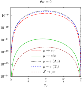
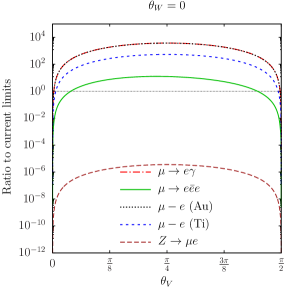
Figure 4: $\mu$ to $e$ transitions as a function of the $\theta_{V}$ mixing angle. The other LHT parameters are fixed to their default values in Eq. (4) and the text. On the left we plot the branching ratios for the different processes while on the right the branching ratios are normalized to the corresponding experimental limits. Note that in the right-hand plot $\mu\to e\gamma$ and $\mu-e\,({\rm Au})$ overlap.

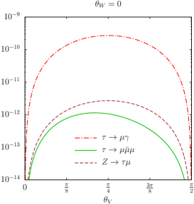
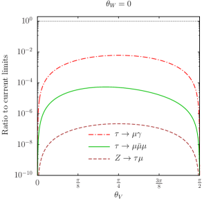
Figure 5: $\tau$ to $\mu$ transitions as a function of the $\theta_{V}$ mixing angle. The other LHT parameters are fixed to their default values in Eq. (4) and the text. On the left we plot the branching ratios for the different processes while on the right the branching ratios are normalized to the corresponding experimental limits.

On the right panel we also show the branching ratios normalized to their current experimental limits in Table 1 which illustrates the sensitivity of the different processes. The first obvious observation about the behavior of the predictions of the LHT is that if the T–odd leptons are aligned with the SM ones, there is no LFV. For vanishing mixing $\theta_{V,W}=0,\pi/2$, all of the LFV transitions go to zero. We see in Figure 4 the largest branching ratios correspond to $\mu-e$ conversion in nuclei and to $\mu\to e\gamma$ (left panel) and at the same time they are also the best measured (right panel). In contrast, limits from on-shell $Z$ and Higgs decays are much less restrictive. In particular, Higgs decays are outside of the left panel and omitted in the following. Furthermore, the anomalous magnetic moment $a_{\mu}$, which is flavor conserving and not sensitive to the mixing entering through $V$ and $W$, is more than two orders of magnitude below present sensitivity. As can be observed in both panels, muon decay into three electrons shows an asymmetric dependence on the $\theta_{V}$ mixing angle. This is in fact the generic behavior of all the observables when we vary the default values. In Figure 5 we plot the same decays as in Figure 4 but for $\tau-\mu$ (being similar the plots for processes involving $\tau-e$ mixing). Comparing both figures, it is apparent how much less restrictive $\tau$ data is as all predictions for $\tau$ decays are below their current experimental limits (see right panel in Figure 5). Thus, in what follows we concentrate on $\mu-e$ transitions.

Once $f$ is fixed, the size of the LFV processes is largely determined by the masses of the mirror and partner mirror leptons. This is apparent from Figure 6 where we plot the branching ratios normalized to their current experimental limits for the different $\mu-e$ processes as a function of the product of mirror masses $\tilde{x}$ for vanishing $\theta_{W}$ in the left panel and of the product of partner mirror masses $\tilde{y}$ for vanishing $\theta_{V}$ in the right one.

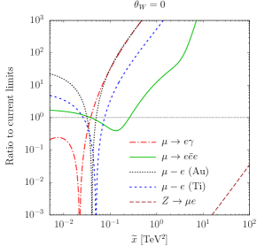
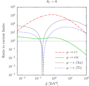
Figure 6: Ratios of the $\mu$ to $e$ transition branching ratios normalized to the corresponding experimental limits as a function of $\tilde{x}$ and $\tilde{y}$ as defined in Eq. (4) for the mirror and partner leptons. On the left (right) we neglect the $\theta_{W(V)}$ mixing. The other LHT parameters are fixed to their default values as defined in Eq. (4). On the right panel $Z\rightarrow\mu e$ lies outside the plot.

Comparing both panels one can also observe the different dependence on the mirror and partner mirror leptons which reflects the different dependence of the observables on the heavy fermion masses. In the left (right) panel there is a clear structure depending on the mirror (partner mirror) lepton masses showing that the corresponding branching ratios can vanish if there is a parameter conspiracy leading to large cancellations. These cancellations require a sharp correlation between the parameters as seen in the narrowness of the vanishing regions. Similar comments apply to Figure 7 although the dependence on $\delta_{\ell_{H}}$ is flat in the left panel as long as it is small while there is no available cancellation varying $\delta_{\tilde{\nu}^{c}}$ in the right panel for the values assumed for the other parameters.

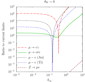
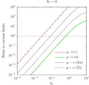
Figure 7: Ratios of the $\mu$ to $e$ transition branching ratios normalized to the corresponding experimental limits as a function of $\delta_{\ell_{H}}$ (left) and $\delta_{\tilde{\nu}^{c}}$ (right) as defined in Eq. (4) for the mirror and partner leptons. On the left (right) we neglect the $\theta_{W(V)}$ mixing while the other LHT parameters are fixed to the default values in Eq. (4).

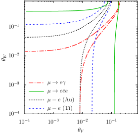
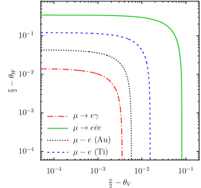
Figure 8: Mixing in the $\theta_{V}-\theta_{W}$ plane required to saturate the current bounds on $\mu$ to $e$ transition branching ratios. Different panels illustrate the different correlation between the two angles depending on where zero or $(\theta_{V},\theta_{W})=(\pi/2,\pi/2)$ is chosen for expanding the misalignment. The other LHT parameters are fixed to their default values in Eq. (4). The remaining processes are below present experimental limits for any mixing angle value.

Finally, in Figure 8 we plot contours in the mixing angle plane which saturate the current experimental limits for LFV processes having sufficient sensitivity. We show two cases corresponding to expanding the misalignment around zero (left) or $(\theta_{V},\theta_{W})=(\pi/2,\pi/2)$ (right). The other model parameters are fixed to the default values in Eq. (4). As can be seen, $\mu\to e\gamma$ decay and $\mu-e$ conversion in Au provide the most stringent constraints. We also see that current limits require the misalignment between the SM and the mirror and partner mirror leptons to be $\sim 1$ % as can be inferred from the $\theta_{V,W}$ values when the curves flatten near the axes. For $\mu\to e$ conversion in nuclei we see similar shaped contours for Au and Ti, with Ti being less restrictive, while $\mu\to e\bar{e}e$ allows the misalignment to be generically $\sim 10$ times larger. For misalignment around zero (left), the mixing angles can be larger if $\theta_{V,W}$ are correlated to equally high precision. For misalignment around $(\theta_{V},\theta_{W})=(\pi/2,\pi/2)$ (right) the mixing angles are always constrained to be small, in particular by $\mu\to e\gamma$.

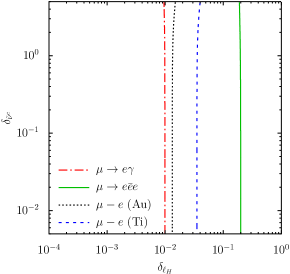
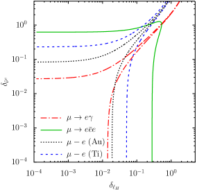
Figure 9: Contours in the $\delta_{\ell_{H}}-\delta_{\tilde{\nu}^{c}}$ plane which saturate the current bounds on $\mu$ to $e$ branching ratios and conversion rates. The left (right) panel corresponds to $\theta_{V,W}=\pi/4\;(\pi/8)$ while the remaining LHT parameters are fixed to the default values given in Eq. (4). The remaining processes are below present experimental limits for the range of mass (squared) splittings considered.

Similar comments apply when studying the dependence on the mirror and partner lepton masses and a similar precision is needed to fit current experimental data from LFV processes. In Figure 9 we show the corresponding contours in the $\delta_{\ell_{H}}-\delta_{\tilde{\nu}^{c}}$ (see Eq. (4)) plane which saturate current experimental limits. With the default values in Eq. (4) chosen for the remaining parameters we see in the left hand panel that there is essentially no dependence on $\delta_{\tilde{\nu}^{c}}$ but $\delta_{\ell_{H}}$ must be tiny, $\sim 1$ % to fulfill the bound from $\mu\to e\gamma$. This asymmetric behavior is due to the choice of mixing angles $\theta_{V,W}=\pi/4$ since for $\theta_{V}+\theta_{W}=\pi/2$ the partner fermion contribution to the relevant LFV processes is much smaller than the mirror one. This is made apparent in the right hand panel where we plot the corresponding contours for $\theta_{V,W}=\pi/8$. As we saw for the mixing angles, the $\mu\to e\gamma$ decay requires the mass (squared) splitting parameter to be tuned within 1 % with analogous behavior in $\mu\to e$ conversion while again for $\mu\to e\bar{e}e$ limits are $\sim 10$ times weaker.

The tuning of the mass splittings and mixing angles required by $\mu$ to $e$ transitions can also be quantified using the measure defined in Barbieri:1987fn in order to compare with other new physics scenarios. Applying it to $\mu\rightarrow e\gamma$ in Figure 7,

$$\Delta=\left|\frac{\partial\ln{\rm Br}(\mu\rightarrow e\gamma)}{\partial\ln\delta_{\ell_{H}}}\right|\,,$$ (45)

we obtain $\Delta\sim 70$ which corresponds to a fine tuning of $\Delta^{-1}\sim 1.4$ % for the two points around $\delta_{\ell_{H}}\sim 0.35$ where the branching ratio saturates the current experimental limit. Though this can be accommodated in the LHT by fixing the parameters appropriately and there are large regions of parameter space in agreement with data, it would be more interesting to complete the LHT with a flavor symmetry which could align the first two heavy lepton families with the $e$ and $\mu$ families of the SM. Explorations of this are left to future work.

As already emphasized and showed in previous figures, the inclusion of the partner mirror lepton contributions enlarge the parameter space allowing for further cancellations but also for the mitigation of possible correlations between LFV observables implied by the mirror lepton contributions previously considered. For illustration, we show in Figure 10 (left) how the scatter plot of the LHT predictions for ${\rm Br}(\mu\rightarrow e\bar{e}e)$ versus ${\rm Br}(\mu\rightarrow e\gamma)$ looks like when only the mirror leptons are considered (green points, in agreement, for example, with Blanke:2009am ; Blanke:2007db ) and when their partners are also included (red and black points).

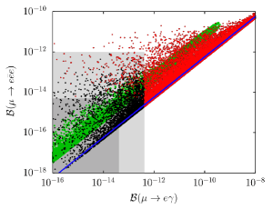
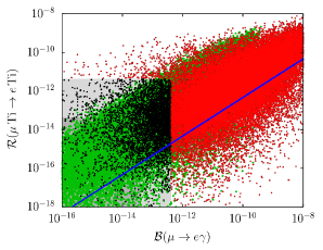
Figure 10: Scatter plots for the LHT contributions to ${\rm Br}(\mu\rightarrow e\bar{e}e)$ versus ${\rm Br}(\mu\rightarrow e\gamma)$ (left) and ${\cal R}(\mu{\rm Ti}\to e{\rm Ti})$ versus ${\rm Br}(\mu\rightarrow e\gamma)$ (right). Green points result from the mirror lepton contributions alone while red and black points result from the mirror and partner mirror contributions together for the parameter values given in the text. But only black points correspond to LHT parameters satisfying the experimental constraints (shaded regions) on the three LFV observables. See the text for further details.

In the right panel we show the corresponding behavior of ${\cal R}(\mu{\rm Ti}\to e{\rm Ti})$ versus ${\rm Br}(\mu\rightarrow e\gamma)$. Black points in both panels correspond to LHT parameter values satisfying the experimental constraints on those three LFV observables. As is apparent in the ${\rm Br}(\mu\rightarrow e\bar{e}e)$ versus ${\rm Br}(\mu\rightarrow e\gamma)$ panel, the existing correlation when only the mirror leptons are taken into account relaxes and the scatter region expands to fill in the experimentally allowed (shaded) area when the partner mirror leptons are also included. Few comments are in order in this case: $i$) The solid (blue) line corresponds to the mirror lepton dipole contribution alone. This contribution is smaller than the mirror lepton $Z$ penguin and box contributions what explains the distance between this solid line and the green region. $ii$) In contrast, the red and black scatter region contains the solid (blue) line. This is because when all the T–odd (non-singlet) lepton contributions are included the dipole term is typically larger, as the $Z$ penguin and box terms, and they also in general interfere. A consequence of this wider range of predictions is the difficulty of distinguishing between the LHT and the corresponding supersymmetric predictions, in contrast with what was previously argued in the absence of partner mirror leptons. For comparison with Refs. Blanke:2009am ; Blanke:2007db we have varied

$$300\ {\rm GeV}\leq m_{\ell_{H1,2}},m_{\tilde{\nu}^{c}_{1,2}}, m_{d_{H1}},m_{\tilde{u}_{1}}\leq 1.5\ {\rm TeV}\ ,$$

$$\theta_{V,W}\in [0,\pi/2)\;,\quad\quad$$ (46)

assuming no heavy quark mixing. The scatter points are accumulated in the most probable observable region but an unweighted scatter plot may be misleading because the less probable and then unpopulated region may not be parametrically forbidden. As a matter of fact, in order to better illustrate what is going on we have weighted the scanned angle intervals logarithmically. This populates the region for small observable values, which is the physically relevant one, and explains why the green region penetrates the very low observable area in contrast with previous scatter plots Blanke:2009am ; Blanke:2007db ). The darker shadow area defines the zone expected to be experimentally allowed in the near future. Besides, we have fixed $f=1.5$ TeV, contrary to the previous scatter plots, where $f$ was assumed to be equal to 1 TeV. Obviously, the LHT predictions can be made as small as needed not only increasing $f$ but taking the mixing angles or the mass differences small enough (see Figs. 4 and 9). This should be also interpreted as fine tuning, in agreement with our conclusion that the misalignment between the T–odd and the SM leptons must be $\sim 1$ % when the other LHT parameters are fixed to their default values, as shown in Fig. 8. Finally, it is also worth noting that the bottom right region which is unpopulated in the left panel, corresponding to ${\rm Br}(\mu\rightarrow e\gamma)/{\rm Br}(\mu\rightarrow e\bar{e}e)\geq 218$, is inaccessible for any value of the form factors involved in their decay widths in Eqs. (11) and (3.1), respectively. The observation of these two processes in this region could not be explained by the LHT contributions considered here nor by any model which could be described by the form factors in Eqs. (10) and (20–23), respectively, at low energy.

For completeness, we have also introduced and varied the CP violating phase present in the general two family case analysed. While $V$ in Eq. (43) can be made real by a proper fermion field redefinition, $W$ is in general complex,

$$W=\begin{bmatrix}\cos\theta_{W}&\sin\theta_{W}e^{i\eta}\\ -\sin\theta_{W}e^{-i\eta}&\cos\theta_{W}\end{bmatrix}\,.$$ (47)

No significant modification of Fig. 10 is found varying $\eta$, although a given subset of predictions (and cancellations) can correspond to different points in parameter space. In any case we have not tried to characterize the full parameter space allowed by experiment, what is beyond the scope of the paper.

5 Future prospects

Future improvements of limits from LFV processes Baldini:2018uhj will shed further light on the LHT model and to what degree it is natural. An improvement of sensitivity in measurements of $\mu\rightarrow e\gamma$ by an order of magnitude, as envisioned by the MEG Collaboration Baldini:2018nnn ; Nakao:2018hip , would increase the required tuning of the heavy lepton alignment by a factor of 1/3. Meanwhile an improvement of the sensitivity in $\mu\to e\bar{e}e$ by more than two orders of magnitude, as expected in Phase I of the Mu3e experiment Perrevoort:2018ttp , would match the tuning currently required by $\mu\rightarrow e\gamma$. Further improving it by almost two orders of magnitude in Phase II Blondel:2013ia would result in a required alignment of the lepton sector at the per mille level or in a new physics scale $f>30$ TeV in the absence of any alignment or accidental cancellation. Experiments on $\mu\to e$ conversion in nuclei are also expected to improve their sensitivity Abusalma:2018xem ; Angelique:2018svf ; Teshima:2018msm . The Mu2e and COMET experiments aim to improve by two to more than four orders of magnitude in two phases. We summarize these prospects for future LFV experiments using intense muon beams in Table 11.

Process	Experiment	$\begin{array}[]{c}{\rm Current}\\[-2.84544pt] {\rm precision}\end{array}$	$\begin{array}[]{c}{\rm Sensitivity}\\[-2.84544pt] {\rm improvement}\end{array}$	$f$ [TeV] $>$		$\begin{array}[]{c}{\rm Mixing\;angle}\\[-2.84544pt] <\times 10^{-2}\end{array}$
$\mu\to e\ \gamma$	[MEG]	$10^{-4}$	$10-500$	$15$	$27-71$	$1$	$0.3-0.04$
$\mu\to e\ \overline{e}\ e$	[Mu3e]	$0.04$	$200-10^{4}$	$3.4$	$13-34$	$20$	$1-0.3$
$\mu\to e\ ({\rm Al})$	[Mu2e]	$10^{-3}$	$10^{4}-10^{5}$	$8.4$	$84-150$	$3$	$0.03-0.01$
$\mu\to e\ ({\rm Al})$	[COMET]	$10^{-3}$	$10^{2}-10^{4}$	$8.4$	$27-84$	$3$	$0.3-0.03$

Table 11: Current precision and projected sensitivity improvement in Phase I–II for different LFV experiments Baldini:2018uhj . In the absence of a signal the corresponding limits on the new physics scale $f$ (for order 1 mixing) and on the mixing angle of the heavy leptons with the first two families (for $f=1.5$ TeV) are shown in the last two columns.

The current precision is estimated by dividing the predictions in Table 1 by the limits in Table 10, while limits on the new physics scale $f$ and alignment of the T–odd lepton with the first two SM families $\theta$ are obtained using the corresponding scaling dependence of the LFV processes for small mixing, $\theta^{2}/f^{4}$.

In the case of $\tau$ decays experimental bounds are less restrictive but constrain other mixings. Belle II Kou:2018nap aims to improve the precision to $10^{-9}-10^{-10}$ in a variety of LFV processes Liventsev:2018gin while LHCb also expects to reach a similar sensitivity Bediaga:2018lhg . The upper bound on $\tau\to\mu\overline{\mu}\mu$ from LHCb Aaij:2014azz is already within a factor of 2 of its current best limit Tanabashi:2018oca (see also DeBruyn:2017aqu for the LHC collaborations). For the default values in Eq. (4) we find that $\tau\rightarrow\mu\gamma$ could constrain the corresponding mixing angles in the LHT (see Table 10 for an estimate) but $\tau\to\mu\bar{\mu}\mu$ will likely not reach the necessary precision to test the LHT prediction of $\Gamma(\tau\to\mu\bar{\mu}\mu)/\Gamma(\tau\rightarrow\mu\gamma)\sim 2\times 10^{-3}$ which we note is similar to predictions in supersymmetric models Ellis:2002fe ; Babu:2002et ; Brignole:2004ah (see also Arganda:2005ji and Dassinger:2007ru ). This is in contrast to previous studies Blanke:2009am ; Blanke:2007db which found that three-body $\tau$ decays could distinguish clearly between the LHT and supersymmetric models. However, these studies only included effects from the mirror leptons as they worked in the limit of decoupled partner leptons. When the contributions from both the mirror and partner leptons are included one finds that there are regions of parameter space where the LHT and supersymmetric predictions are similar. Thus these decays cannot unambiguously distinguish between these two models.

To understand this further we recall that the supersymmetric prediction Ellis:2002fe ; Babu:2002et ; Brignole:2004ah relies on the observation that when the photon dipole contribution dominates the three-body $\tau$ decay, the ratio to the corresponding radiative two-body $\tau$ decay in Eq. (11) is fixed by kinematics,

$$\frac{\rm Br(\ell\to\ell^{\prime}\overline{\ell^{\prime}}\ell^{\prime})}{\rm Br(\ell\to\ell^{\prime}\gamma)}=\frac{\alpha}{3\pi}\left(2\ln\frac{m_{\ell}}{m_{\ell^{\prime}}}-\frac{13}{4}\right)\,,\;\;\frac{\rm Br(\ell\to\ell^{\prime}\overline{\ell^{\prime\prime}}\ell^{\prime\prime})}{\rm Br(\ell\to\ell^{\prime}\gamma)}=\frac{\alpha}{3\pi}\left(2\ln\frac{m_{\ell}}{m_{\ell^{\prime\prime}}}-\frac{7}{2}\right)\,.$$ (48)

In the LHT the photon dipole term is the one proportional to $|A_{R}|^{2}$ in Eqs. (3.1) and (3.1) so in regions of parameter space where this term dominates, the LHT prediction will also be fixed by kinematics and thus similar to the supersymmetric prediction. In the left panel of Figure 11 we plot the ratio $\Gamma(\tau\to\mu\overline{e}e)/\Gamma(\tau\to\mu\overline{\mu}\mu)$ (see Eqs. (3.1) and (3.1), respectively) as a function of the mass product parameter $\tilde{x}$ for the default values of the other LHT parameters fixed in Eqs. (4). We show the prediction when all T–odd (non-singlet) leptons, $l_{H}$ and $\tilde{l}$, are included (solid line) and when only the mirror leptons, $l_{H}$, are taken into account (dashed line).

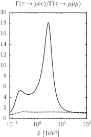
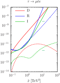
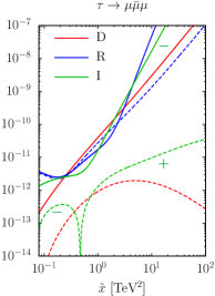
Figure 11: Left: LHT prediction for the ratio ${\Gamma(\tau\to\mu\overline{e}e)}/{\Gamma(\tau\to\mu\overline{\mu}\mu)}$ as a function of $\tilde{x}=m_{\ell_{H2}}m_{\ell_{H3}}$ for $\tau-\mu$ mixing, with the remaining parameters fixed to their default values Eq. (4). The solid line shows the prediction when both mirror and partner mirror leptons ($l_{H}$ and $\tilde{l}$) are included while the dashed shows when only the mirror leptons ($l_{H}$) are taken into account. Middle and Right: LHT model predictions for ${\Gamma(\tau\to\mu\overline{e}e)}$ and ${\Gamma(\tau\to\mu\overline{\mu}\mu)}$ separating the photon dipole contribution (D), the other form factor contributions (R), and their interference (I).

As can be seen, when only the mirror leptons are taken into account (dashed line) there is no logarithmic enhancement from the photon dipole term while when the partner leptons are also included (solid line) the logarithmic enhancement in Eq. (48) is significant. How large it is of course depends on the particular choice of parameters. To illustrate this we compare the predictions in Table 12 for ${\rm Br(\tau\to\mu\overline{\mu}\mu)}/{\rm Br(\tau\to\mu\gamma)}$ and ${\rm Br(\tau\to\mu\overline{e}e)}/{\rm Br(\tau\to\mu\gamma)}$ in supersymmetric models assuming the photon dipole dominates (see Eq. (48)) and the LHT model for the default values of the parameters in Eq. (4) when all T–odd (non-singlet) leptons ($l_{H}$ and $\tilde{l}$) are included and when only the mirror leptons ($l_{H}$) are included with the partner leptons decoupled.

Ratio	SUSY	LHT ($l_{H}+\tilde{l}$)	LHT ($l_{H}$)
$\frac{\rm Br(\tau\to\mu\overline{\mu}\mu)}{\rm Br(\tau\to\mu\gamma)}$	$1.9\times 10^{-3}$	$1.9\times 10^{-3}$	$6.0\times 10^{-2}$
$\frac{\rm Br(\tau\to\mu\overline{e}e)}{\rm Br(\tau\to\mu\gamma)}$	$9.9\times 10^{-3}$	$1.1\times 10^{-2}$	$7.5\times 10^{-2}$

Table 12: Predictions for ratios of $\tau$ decays in supersymmetric models when the photon dipole dominates and in the LHT model assuming the default values for the parameters in Eq. (4) when including all T–odd (non-singlet) leptons ($l_{H}$ and $\tilde{l}$) and when including only the mirror ones ($l_{H}$).

From Table 12 we see the prediction for the ratio of the two ratios is $\sim 5$ in both supersymmetric models and, for the parameter point with $\tilde{x}=1\,{\rm TeV}^{2}$, in the LHT model when including $l_{H}$ and $\tilde{l}$ while the ratio of ratios is $\sim 1$ when only the $l_{H}$ are included. Thus we see that for parameter points near $\tilde{x}=1\,{\rm TeV}^{2}$, the LHT gives predictions similar to supersymmetric models when the mirror and partner leptons are included while they differ significantly when only mirror leptons are taken into account. As can be deduced from Figure 11 (left panel), when both $l_{H}$ and $\tilde{l}$ are included, this ratio of ratios decreases rapidly starting from $\tilde{x}\sim{\rm TeV}^{2}$ and converges to $\sim 1$ as $\tilde{x}$ becomes large. The behavior around $\tilde{x}=1\,{\rm TeV}^{2}$ can be better understood by examining $\Gamma(\tau\to\mu\overline{e}e)$ and $\Gamma(\tau\to\mu\overline{\mu}\mu)$ and separating it into the photon dipole contribution (D) the contribution from other form factors (R) and the contribution from their interference (I) which we show in Figure 11 (middle and right panels, respectively). When only the mirror leptons are included (dashed lines) the photon dipole contribution is rather small and $\Gamma(\tau\to\mu\overline{e}e)$ and $\Gamma(\tau\to\mu\overline{\mu}\mu)$ are almost equal (the $\pm$ on the interference term (dashed line) indicates the overall sign). When the partner leptons are also taken into account (solid lines) the photon dipole contribution dominates in the region around $\tilde{x}\sim 1\,{\rm TeV}^{2}$. The strong dependence on $\tilde{x}$ seen in Figure 11 in this region can be traced back to the behavior of the loop functions in Eq. (3.1) and, in particular, the charged partner lepton loop function $F^{\tilde{\ell}}_{M}(x)$. Thus we see how when all the heavy T–odd leptons are included, supersymmetric models and the LHT model cannot be unambiguously distinguished utilizing three-body $\tau$ decays.

Finally, it is also important to emphasize that future leptonic colliders will produce a large number of Drell–Yan lepton pairs and in particular $\overline{\tau}\tau$. A potentially promising probe of LFV in the LHT at $e\overline{e}$ colliders is searching for $\overline{\ell^{\prime}}\ell^{\prime\prime}$ production (for a recent review of LFV $\tau$ decays at the FCC-ee see Dam:2018rfz ). For illustration, in Fig. 12 we show the prediction for $e\overline{e}\to\overline{\tau}\mu$ (left panel) and its ratio to $e\overline{e}\to\overline{\tau}\tau$ (right panel) as a function of the center of mass energy squared ($s=Q^{2}$) for different mixing angles and for the default values of the remaining LHT parameters in Eqs. (4).

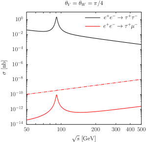
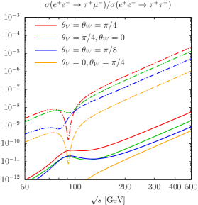
Figure 12: LHT predictions for $e\overline{e}\to\overline{\tau}\mu$ (left panel) and its ratio to $e\overline{e}\to\overline{\tau}\tau$ (right panel) as a function of the center of mass energy squared ($s=Q^{2}$) for different mixing angles $\theta_{V,W}$ and for the default values in Eqs. (4) for the other LHT parameters. Solid (dashed-dotted) lines correspond to $\tilde{x}=1$ TeV² (10 TeV²).

For our estimate we use the amplitude in Eq. (20) which after crossing reads:

$${\cal M}^{\ell\overline{\ell}\to\overline{\ell^{\prime}}\ell^{\prime\prime}} =\,\overline{v}(p_{\overline{\ell}})\,\gamma_{\mu}\,e\,u(p_{\ell})\,\frac{1}{Q^{2}}\,\overline{u}(p_{\ell^{\prime\prime}})\,e\,F_{L}^{\gamma}(Q^{2})\,\gamma^{\mu}P_{L}\,v(p_{\overline{\ell^{\prime}}})$$

$$+ \,\overline{v}(p_{\overline{\ell}})\,\gamma_{\mu}\,(g_{L}^{Z}P_{L}+g_{R}^{Z}P_{R})\,u(p_{\ell})\,\frac{1}{Q^{2}-M_{Z}^{2}+iM_{Z}\Gamma_{Z}}\,\overline{u}(p_{\ell^{\prime\prime}})\,e\,F_{L}^{Z}(Q^{2})\,\gamma^{\mu}P_{L}\,v(p_{\overline{\ell^{\prime}}})$$

$$+ \,e^{2}B_{L}(0)\,\overline{v}(p_{\overline{\ell}})\,\gamma^{\mu}P_{L}\,u(p_{\ell})\,\overline{u}(p_{\ell^{\prime\prime}})\,\gamma_{\mu}P_{L}\,v(p_{\overline{\ell^{\prime}}})\ ,$$ (49)

resulting in a cross section

$$\sigma(e\overline{e}\to\overline{\tau}\mu) =\frac{\pi\alpha^{2}}{3s}\left\{2\,|F_{L}^{\gamma}(s)|^{2}+\frac{(g_{L}^{Z})^{2}+(g_{R}^{Z})^{2}}{e^{2}}|F_{L}^{Z}(s)|^{2}|\chi_{Z}(s)|^{2}+{s^{2}}|B_{L}|^{2}\right.$$ (50)

$$+ \left.\left[F_{L}^{\gamma}(s)\left(\frac{g_{L}^{Z}+g_{R}^{Z}}{e}F_{L}^{Z*}(s)\chi^{*}_{Z}(s)+sB_{L}^{*}\right)+\frac{g_{L}^{Z}}{e}F_{L}^{Z}(s)\chi_{Z}(s)sB_{L}^{*}+\,{\rm h.c.}\right]\right\}\,,$$

with $\chi_{Z}(s)=s(s-M_{Z}^{2}+iM_{Z}\Gamma_{Z})^{-1}$.

As is apparent from Fig. 12 (left panel) where we plot the total cross-section for $e\overline{e}\to\overline{\tau}\mu$ and $e\overline{e}\to\overline{\tau}\tau$, the LFV cross-section grows with energy. When the box diagram contributions are large, no $Z$ peak emerges (dashed-dotted line corresponding to $\tilde{x}=10\,{\rm TeV}^{2}$) in the invariant mass spectrum which opens up the possibility that a large enough LFV production cross-section can be observable without being excluded by $Z$-pole measurements. On the right hand panel we show the variation of this cross-section with the mixing angles which we see can be almost two orders of magnitude for ${\cal O}(1)$ mixing. The growth with $s$ of the cross-section $e\overline{e}\to\overline{\tau}\mu$ below the production threshold of new (T–odd) particles reflects the fact that, in the presence of a mass gap, any extension of the SM can be described at low energy by effective operators of dimension 6 at leading order. Then, as they are suppressed by the large new physics scale squared ($f^{-2}$), their contributions must grow with the low energy scale $s$ (see Eq. (50)). This is a sensible approximation in our case (with the T–odd particles near the TeV) for $\sqrt{s}\leq 500$ GeV. Above the resonance region, for much larger $s$ values, the LHT penguin and box diagram contributions scale like $s^{-1}$ and hence, the cross-section also decreases as $s^{-1}$, satisfying the unitarity bound. To summarize, although for the default values of the parameters it may be difficult to observe LFV events, in other regions of parameter space it will be possible to constrain the $\tau$ sector in the LHT at a future FCC-ee Benedikt:2018qee or ILC Baer:2013cma machine assuming $\mathcal{O}(10^{11})$ $\overline{\tau}\tau$ pairs are collected. As noted in footnote 24 these regions can be compatible with current constraints on LFV $\tau$ decays. Thus, considering the huge statistics available at future lepton colliders, it will be worthwhile to study the detectability of such signals in detail.

6 Conclusions

The LHT is an elegant and phenomenologically viable example of a composite Higgs model with improved radiative behavior due to its T–parity which helps mitigate the flavor hierarchy problem significantly. This discrete symmetry also requires the heavy T–odd spectrum to be pair-produced allowing their masses to be $\mathcal{O}(\rm{TeV})$ without violating present direct and indirect constraints. In this study we have revised the constraints on the T–odd spectrum of the LHT implied by present bounds on LFV processes. We have completed previous phenomenological analyses in two ways: First, we have included for the first time all contributions from the full electroweak charged T–odd sector and in particular, the T–odd partner leptons previously neglected in phenomenological studies of low momentum transfer LFV processes. As we have discussed, lepton electroweak singlets can be safely omitted in this phenomenological analysis. Second, we have computed on-shell LFV $Z$ decays which, along with calculations of on-shell LFV Higgs decays delAguila:2017ugt , completes the set of observables at both small and large momentum transfers needed to analyze LFV in the LHT. We have compared these predictions with experiment for all available LFV processes in Table 1. The $\mu-e$ and $\tau-\mu$ and $\tau-e$ sectors are studied separately assuming a two-family description for each. The general case can be obtained combining the parameters of the three analyses, noting that the restrictions on the $\tau-e$ sector are virtually identical to those on $\tau-\mu$ (see Table 1).

For the $\tau-\mu$ LFV observables we find that low energy observables, namely $\tau\to\mu\gamma$ and $\tau\to\mu\overline{\mu}\mu$, are much more restrictive than on-shell LFV decays of the $Z$ or Higgs bosons which are typically orders of magnitude below the current limits. We also find that even when allowing low energy observables to saturate their current experimental limits, on-shell LFV $Z$ and Higgs decays can be at most $\mathcal{O}(10^{-7})$. The pattern of LFV is quite similar for $\tau-e$ transitions with small differences due to the slightly different experimental bounds.

On the other hand, $\mu-e$ transitions present significant differences. First, Higgs decays are proportional to the masses of the SM leptons in the final state and are therefore strongly suppressed for decays not involving the $\tau$ lepton. In general constraints on $\mu-e$ transitions from low energy LFV observables are very strong and render on-shell $Z$ or Higgs decays to $\mu e$ too small to be observable even in future experiments. Furthermore, there is very little correlation between the different low-energy LFV observables so the only way of generically satisfying $\mu-e$ constraints is by reducing the global suppression factor by means of a relatively large $f$ and/or small mixing angles since even with the new source of flavor violation, cancellations are far from generic. This implies large global symmetry breaking scales $f>10$ TeV or small mixing angles $\theta_{V,W}<10^{-2}$.

Motivated by considerations of naturalness, we have focused our phenomenological studies on the case of small mixing angles and/or accidental cancellations with $f=1.5$ TeV. We have explicitly shown that although all current bounds can be satisfied with small mixing angles, some of them can be the result of accidental cancellations between the new contributions to these processes. Furthermore, we have quantified the amount of fine tuning necessary and found it to be $\sim 1$ % for particular parameter points. While the LHT can accommodate limits from searches of FCNC, a flavor completion of the model with a natural suppression of the leptonic FCNC would be welcome.

Future LFV experiments using intense muon beams will typically improve the current sensitivity by two to four orders of magnitude, constraining the effective $\mu-e$ mixing to 1 per mille for $f\gtrsim$ TeV in the absence of a signal. In this case, future LFV experiments will strongly challenge the LHT scenario probing scales $f\sim 10$ TeV even for mixings of order 1 %, thus pushing the concept of naturalness in the LHT to its limits. We have also shown, in contrast to previous studies, that in certain regions of parameter space the LHT model can give similar predictions to supersymmetric models for LFV processes. In other LHT parameter regions $\tau$ LFV transitions can saturate current experimental bounds and hence, can be observed at Belle II as well as the LHC and/or future lepton colliders. As the current sensitivity on $\tau$ LFV processes does not favor any definite pattern of $\tau$ mixing, a systematic study of $\tau\mu$ and $\tau e$ production is worthwhile.

Appendix A Flavor conserving observables

For $\ell^{\prime}=\ell$ the vertex in Eq. (10) allows to define the anomalous magnetic and the electric dipole moments of the $\ell$ lepton,

$$a_{\ell}\equiv\frac{(g-2)_{\ell}}{2}=2\,m_{\ell}F_{M}^{\gamma}(0)\ \quad{\rm and}\ \quad d_{\ell}=-eF_{E}^{\gamma}(0)\ ,$$ (51)

respectively, where both moments are real if the interaction is to be Hermitian (see, for instance, Branco:1999fs ). The contribution of the T–odd spectrum in the LHT to $F_{M}^{\gamma}(0)$ and hence, its contribution to $a_{\ell}$ just defined, can be read from Eq. (3.1). It is real by inspection: the loop functions are real because only heavy particles far away from any physical threshold run in the loops, and the mixing matrix elements as well as their complex conjugates enter symmetrically.

On the other hand the contribution of these T–odd particles to the real part of $F_{E}^{\gamma}(0)$ (and then to $d_{\ell}$) vanishes because the form factors satisfy $F_{E}^{\gamma}(0)=iF_{M}^{\gamma}(0)$ and thus, are purely imaginary. Indeed, from Eq. (3.1)

$$d_{e}=e\ {\rm Im}F_{M}^{\gamma}(0)=e\sum_{i,j,k}\frac{{\rm Im}(V^{*}_{ie}W^{*}_{ji}W_{jk}V_{ke}+V^{*}_{ke}W^{*}_{jk}W_{ji}V_{ie})}{2}\ G_{ijk}=0\;,$$ (52)

where the first term of that equation combining the real products $V^{*}_{ie}V_{ie}$ is also real and the second term involving $V^{*}_{ie}W^{*}_{ji}W_{jk}V_{ke}$ products multiplied by a real function $G_{ijk}$ symmetric under the exchange of the mirror leptons $i$ and $k$ can be reordered as above to make the sum explicitly real. The current experimental precision $|d_{e}|<1.1\times 10^{-29}\ e\cdot$cm at 90% C.L. Andreev:2018ayy deserves a full two-loop calculation Barr:1990vd , what is beyond the scope of this paper. It is worth emphasizing, however, that: $i$) One-loop dimension 6 operators contributing to $d_{e}$ via mixing Panico:2018hal can be generated exchanging T–odd (non-singlet) leptons, but only through triangular diagrams. In particular, no box diagram can be closed to generate the dimension 6 operator $|\phi|^{2}V^{\mu\nu}\tilde{V}_{\mu\nu}$, with $\phi$ the SM Higgs doublet (of hypercharge 1/2), $V^{\mu\nu}$ an electro-weak gauge boson field strength and $\tilde{V}_{\mu\nu}$ its dual tensor, because there is no trilinear coupling of the Higgs doublet to two T–odd lepton doublets. On the other hand there is a quartic coupling with two Higgs doublets to two T–odd lepton doublets, $(\overline{l_{HL}}\tilde{\phi})(\tilde{\phi}^{\dagger}l_{HR})+{\rm h.c.}\supset\frac{1}{4}h^{2}\overline{\nu_{H}}\nu_{H}$, with $\tilde{\phi}=i\sigma^{2}\phi^{*}$, delAguila:2017ugt which can be inserted in a (triangular) fermionic loop emitting two SM gauge bosons, none of them being a photon. $ii$) In contrast, we expect non-vanishing box (and triangular) contributions when considering the quark sector, not studied here, because this also includes T–odd electro-weak quark singlets. In any case, we can use the rough estimate in Panico:2018hal ,

$$\frac{d_{e}}{e}\simeq\left(\frac{g^{2}}{16\pi^{2}}\right)^{2}\frac{m_{e}}{f^{2}}\sin\vartheta\;,$$ (53)

to obtain a bound on the effective CP violating phase $|\sin\vartheta|<0.34$ for $f=1.5$ TeV (and $g=0.65$). What is a milder fine tuning compared to the 1 % alignment of the T–odd (non-singlet) leptons with the SM ones required by current limits on LFV processes involving the first two families. $iii$) A discussion of the sub-leading contributions from dimension 8 operators is also necessary Panico:2018hal .

References

- (1) S. Chatrchyan et al. [CMS Collaboration], Phys. Lett. B 716 (2012) 30 doi:10.1016/j.physletb.2012.08.021 [arXiv:1207.7235 [hep-ex]].
- (2) G. Aad et al. [ATLAS Collaboration], Phys. Lett. B 716 (2012) 1 doi:10.1016/j.physletb.2012.08.020 [arXiv:1207.7214 [hep-ex]].
- (3) A. Falkowski, F. Riva and A. Urbano, JHEP 1311 (2013) 111 doi:10.1007/JHEP11(2013)111 [arXiv:1303.1812 [hep-ph]].
- (4) G. Aad et al. [ATLAS and CMS Collaborations], JHEP 1608 (2016) 045 doi:10.1007/JHEP08(2016)045 [arXiv:1606.02266 [hep-ex]].
- (5) P. W. Graham, D. E. Kaplan and S. Rajendran, Phys. Rev. Lett. 115, no. 22, 221801 (2015) doi:10.1103/PhysRevLett.115.221801 [arXiv:1504.07551 [hep-ph]].
- (6) A. Falkowski, Pramana 87, no. 3, 39 (2016) doi:10.1007/s12043-016-1251-5 [arXiv:1505.00046 [hep-ph]].
- (7) C. Englert, R. Kogler, H. Schulz and M. Spannowsky, Eur. Phys. J. C 76, no. 7, 393 (2016) doi:10.1140/epjc/s10052-016-4227-1 [arXiv:1511.05170 [hep-ph]].
- (8) A. M. Sirunyan et al. [CMS Collaboration], Phys. Lett. B 774 (2017) 533 doi:10.1016/j.physletb.2017.09.083 [arXiv:1705.09171 [hep-ex]].
- (9) M. Aaboud et al. [ATLAS Collaboration], Phys. Rev. D 98 (2018) no.5, 052008 doi:10.1103/PhysRevD.98.052008 [arXiv:1808.02380 [hep-ex]].
- (10) J. de Blas, M. Chala and J. Santiago, Phys. Rev. D 88 (2013) 095011 doi:10.1103/PhysRevD.88.095011 [arXiv:1307.5068 [hep-ph]].
- (11) A. Falkowski and F. Riva, JHEP 1502, 039 (2015) doi:10.1007/JHEP02(2015)039 [arXiv:1411.0669 [hep-ph]].
- (12) J. de Blas, M. Chala and J. Santiago, JHEP 1509 (2015) 189 doi:10.1007/JHEP09(2015)189 [arXiv:1507.00757 [hep-ph]].
- (13) L. Berthier and M. Trott, JHEP 1602, 069 (2016) doi:10.1007/JHEP02(2016)069 [arXiv:1508.05060 [hep-ph]].
- (14) A. Buckley, C. Englert, J. Ferrando, D. J. Miller, L. Moore, M. Russell and C. D. White, JHEP 1604 (2016) 015 doi:10.1007/JHEP04(2016)015 [arXiv:1512.03360 [hep-ph]].
- (15) J. de Blas, M. Ciuchini, E. Franco, S. Mishima, M. Pierini, L. Reina and L. Silvestrini, JHEP 1612 (2016) 135 doi:10.1007/JHEP12(2016)135 [arXiv:1608.01509 [hep-ph]].
- (16) A. Falkowski, M. González-Alonso and K. Mimouni, JHEP 1708 (2017) 123 doi:10.1007/JHEP08(2017)123 [arXiv:1706.03783 [hep-ph]].
- (17) J. Ellis, C. W. Murphy, V. Sanz and T. You, JHEP 1806 (2018) 146 doi:10.1007/JHEP06(2018)146 [arXiv:1803.03252 [hep-ph]].
- (18) C. Grojean, M. Montull and M. Riembau, arXiv:1810.05149 [hep-ph].
- (19) E. d. S. Almeida, A. Alves, N. R. Agostinho, O. J. P. Éboli and M. C. Gonzalez-Garcia, arXiv:1812.01009 [hep-ph].
- (20) N. Arkani-Hamed, A. G. Cohen and H. Georgi, Phys. Lett. B 513 (2001) 232 doi:10.1016/S0370-2693(01)00741-9 [hep-ph/0105239].
- (21) N. Arkani-Hamed, A. G. Cohen and H. Georgi, Phys. Rev. Lett. 86, 4757 (2001) doi:10.1103/PhysRevLett.86.4757 [hep-th/0104005].
- (22) N. Arkani-Hamed, A. G. Cohen, E. Katz and A. E. Nelson, JHEP 0207, 034 (2002) doi:10.1088/1126-6708/2002/07/034 [hep-ph/0206021].
- (23) H. C. Cheng and I. Low, JHEP 0309 (2003) 051 doi:10.1088/1126-6708/2003/09/051 [hep-ph/0308199].
- (24) H. C. Cheng and I. Low, JHEP 0408 (2004) 061 doi:10.1088/1126-6708/2004/08/061 [hep-ph/0405243].
- (25) H. C. Cheng, I. Low and L. T. Wang, Phys. Rev. D 74 (2006) 055001 doi:10.1103/PhysRevD.74.055001 [hep-ph/0510225].
- (26) J. Hubisz, P. Meade, A. Noble and M. Perelstein, JHEP 0601, 135 (2006) doi:10.1088/1126-6708/2006/01/135 [hep-ph/0506042].
- (27) I. Low, JHEP 0410 (2004) 067 doi:10.1088/1126-6708/2004/10/067 [hep-ph/0409025].
- (28) J. Hubisz and P. Meade, Phys. Rev. D 71 (2005) 035016 doi:10.1103/PhysRevD.71.035016 [hep-ph/0411264].
- (29) J. Hubisz, S. J. Lee and G. Paz, JHEP 0606 (2006) 041 doi:10.1088/1126-6708/2006/06/041 [hep-ph/0512169].
- (30) C. R. Chen, K. Tobe and C.-P. Yuan, Phys. Lett. B 640 (2006) 263 doi:10.1016/j.physletb.2006.07.053 [hep-ph/0602211].
- (31) M. Blanke, A. J. Buras, A. Poschenrieder, C. Tarantino, S. Uhlig and A. Weiler, JHEP 0612 (2006) 003 doi:10.1088/1126-6708/2006/12/003 [hep-ph/0605214].
- (32) A. J. Buras, A. Poschenrieder, S. Uhlig and W. A. Bardeen, JHEP 0611 (2006) 062 doi:10.1088/1126-6708/2006/11/062 [hep-ph/0607189].
- (33) A. Belyaev, C. R. Chen, K. Tobe and C.-P. Yuan, Phys. Rev. D 74 (2006) 115020 doi:10.1103/PhysRevD.74.115020 [hep-ph/0609179].
- (34) M. Blanke, A. J. Buras, A. Poschenrieder, S. Recksiegel, C. Tarantino, S. Uhlig and A. Weiler, JHEP 0701 (2007) 066 doi:10.1088/1126-6708/2007/01/066 [hep-ph/0610298].
- (35) C. T. Hill and R. J. Hill, Phys. Rev. D 75 (2007) 115009 doi:10.1103/PhysRevD.75.115009 [hep-ph/0701044].
- (36) C. T. Hill and R. J. Hill, Phys. Rev. D 76 (2007) 115014 doi:10.1103/PhysRevD.76.115014 [arXiv:0705.0697 [hep-ph]].
- (37) X. F. Han, L. Wang and J. M. Yang, Phys. Rev. D 78 (2008) 075017 doi:10.1103/PhysRevD.78.075017 [arXiv:0807.4480 [hep-ph]].
- (38) T. Goto, Y. Okada and Y. Yamamoto, Phys. Lett. B 670 (2009) 378 doi:10.1016/j.physletb.2008.11.022 [arXiv:0809.4753 [hep-ph]].
- (39) F. del Aguila, J. I. Illana and M. D. Jenkins, JHEP 0901 (2009) 080 doi:10.1088/1126-6708/2009/01/080 [arXiv:0811.2891 [hep-ph]].
- (40) M. Blanke, A. J. Buras, B. Duling, S. Recksiegel and C. Tarantino, Acta Phys. Polon. B 41 (2010) 657 [arXiv:0906.5454 [hep-ph]].
- (41) F. del Aguila, J. I. Illana and M. D. Jenkins, JHEP 1009 (2010) 040 doi:10.1007/JHEP09(2010)040 [arXiv:1006.5914 [hep-ph]].
- (42) T. Goto, Y. Okada and Y. Yamamoto, Phys. Rev. D 83 (2011) 053011 doi:10.1103/PhysRevD.83.053011 [arXiv:1012.4385 [hep-ph]].
- (43) H. S. Hou, H. Sun and Y. J. Zhou, Commun. Theor. Phys. 59 (2013) 443 doi:10.1088/0253-6102/59/4/10 [arXiv:1210.3904 [hep-ph]].
- (44) J. Reuter, M. Tonini and M. de Vries, JHEP 1402 (2014) 053 doi:10.1007/JHEP02(2014)053 [arXiv:1310.2918 [hep-ph]].
- (45) B. Yang, J. Han and N. Liu, Phys. Rev. D 95 (2017) no.3, 035010 doi:10.1103/PhysRevD.95.035010 [arXiv:1605.09248 [hep-ph]].
- (46) D. Dercks, G. Moortgat-Pick, J. Reuter and S. Y. Shim, JHEP 1805 (2018) 049 doi:10.1007/JHEP05(2018)049 [arXiv:1801.06499 [hep-ph]].
- (47) M. Schmaltz and D. Tucker-Smith, Ann. Rev. Nucl. Part. Sci. 55 (2005) 229 doi:10.1146/annurev.nucl.55.090704.151502 [hep-ph/0502182].
- (48) M. Perelstein, Prog. Part. Nucl. Phys. 58 (2007) 247 doi:10.1016/j.ppnp.2006.04.001 [hep-ph/0512128].
- (49) G. Panico and A. Wulzer, Lect. Notes Phys. 913 (2016) pp.1 doi:10.1007/978-3-319-22617-0 [arXiv:1506.01961 [hep-ph]].
- (50) S. L. Glashow, J. Iliopoulos and L. Maiani, Phys. Rev. D 2 (1970) 1285. doi:10.1103/PhysRevD.2.1285
- (51) G. Isidori, Y. Nir and G. Perez, Ann. Rev. Nucl. Part. Sci. 60 (2010) 355 doi:10.1146/annurev.nucl.012809.104534 [arXiv:1002.0900 [hep-ph]].
- (52) M. Raidal et al., Eur. Phys. J. C 57 (2008) 13 doi:10.1140/epjc/s10052-008-0715-2 [arXiv:0801.1826 [hep-ph]].
- (53) A. Pich, arXiv:1805.08597 [hep-ph].
- (54) H. Georgi, Phys. Lett. 169B (1986) 231. doi:10.1016/0370-2693(86)90657-X
- (55) L. Alvarez-Gaume, J. Polchinski and M. B. Wise, Nucl. Phys. B 221 (1983) 495. doi:10.1016/0550-3213(83)90591-6
- (56) D. B. Kaplan, Nucl. Phys. B 365 (1991) 259. doi:10.1016/S0550-3213(05)80021-5
- (57) C. Csaki, C. Delaunay, C. Grojean and Y. Grossman, JHEP 0810 (2008) 055 doi:10.1088/1126-6708/2008/10/055 [arXiv:0806.0356 [hep-ph]].
- (58) J. Santiago, JHEP 0812 (2008) 046 doi:10.1088/1126-6708/2008/12/046 [arXiv:0806.1230 [hep-ph]].
- (59) C. Csaki, A. Falkowski and A. Weiler, Phys. Rev. D 80 (2009) 016001 doi:10.1103/PhysRevD.80.016001 [arXiv:0806.3757 [hep-ph]].
- (60) F. del Aguila, A. Carmona and J. Santiago, JHEP 1008 (2010) 127 doi:10.1007/JHEP08(2010)127 [arXiv:1001.5151 [hep-ph]].
- (61) F. del Aguila, L. Ametller, J. I. Illana, J. Santiago, P. Talavera and R. Vega-Morales, JHEP 1708, 028 (2017) doi:10.1007/JHEP08(2017)028 [arXiv:1705.08827 [hep-ph]].
- (62) S. Borsanyi et al. [Budapest-Marseille-Wuppertal Collaboration], Phys. Rev. Lett. 121 (2018) no.2, 022002 doi:10.1103/PhysRevLett.121.022002 [arXiv:1711.04980 [hep-lat]].
- (63) T. Blum et al. [RBC and UKQCD Collaborations], Phys. Rev. Lett. 121 (2018) no.2, 022003 doi:10.1103/PhysRevLett.121.022003 [arXiv:1801.07224 [hep-lat]].
- (64) V. Andreev et al. [ACME Collaboration], Nature 562 (2018) no.7727, 355. doi:10.1038/s41586-018-0599-8
- (65) G. Panico, A. Pomarol and M. Riembau, JHEP 1904 (2019) 090 doi:10.1007/JHEP04(2019)090 [arXiv:1810.09413 [hep-ph]].
- (66) T. Chupp, P. Fierlinger, M. Ramsey-Musolf and J. Singh, Rev. Mod. Phys. 91 (2019) no.1, 015001 doi:10.1103/RevModPhys.91.015001 [arXiv:1710.02504 [physics.atom-ph]].
- (67) G. Panico, M. Riembau and T. Vantalon, JHEP 1806 (2018) 056 doi:10.1007/JHEP06(2018)056 [arXiv:1712.06337 [hep-ph]].
- (68) M. Lindner, M. Platscher and F. S. Queiroz, Phys. Rept. 731 (2018) 1 doi:10.1016/j.physrep.2017.12.001 [arXiv:1610.06587 [hep-ph]].
- (69) F. del Aguila, L. Ametller, J. I. Illana, J.M. Perez-Poyatos, J. Santiago, P. Talavera and R. Vega-Morales, in preparation.
- (70) D. Pappadopulo and A. Vichi, JHEP 1103 (2011) 072 doi:10.1007/JHEP03(2011)072 [arXiv:1007.4807 [hep-ph]].
- (71) M. Tonini, DESY-THESIS-2014-038.
- (72) S. Y. Shim, doi:10.3204/PUBDB-2018-01793
- (73) J. Reuter, D. Dercks, G. Moortgat-Pick and S. Y. Shim, arXiv:1811.02268 [hep-ph].
- (74) L. Vecchi, arXiv:1304.4579 [hep-ph].
- (75) A. Baldini et al., arXiv:1812.06540 [hep-ex].
- (76) D. Liventsev [Belle II Collaboration], PoS NuFact 2017 (2018) 118. doi:10.22323/1.295.0118
- (77) R. Aaij et al. [LHCb Collaboration], arXiv:1808.08865.
- (78) M. Benedikt et al., CERN-ACC-2018-0057.
- (79) H. Baer et al., arXiv:1306.6352 [hep-ph].
- (80) M. Blanke, A. J. Buras, B. Duling, A. Poschenrieder and C. Tarantino, JHEP 0705 (2007) 013 doi:10.1088/1126-6708/2007/05/013 [hep-ph/0702136].
- (81) J. Adam et al. [MEG Collaboration], Phys. Rev. Lett. 110 (2013) 201801 doi:10.1103/PhysRevLett.110.201801 [arXiv:1303.0754 [hep-ex]].
- (82) U. Bellgardt et al. [SINDRUM Collaboration], Nucl. Phys. B 299 (1988) 1. doi:10.1016/0550-3213(88)90462-2
- (83) W. H. Bertl et al. [SINDRUM II Collaboration], Eur. Phys. J. C 47 (2006) 337. doi:10.1140/epjc/s2006-02582-x
- (84) B. Aubert et al. [BaBar Collaboration], Phys. Rev. Lett. 104 (2010) 021802 doi:10.1103/PhysRevLett.104.021802 [arXiv:0908.2381 [hep-ex]].
- (85) M. Tanabashi et al. [Particle Data Group], Phys. Rev. D 98 (2018) no.3, 030001. doi:10.1103/PhysRevD.98.030001
- (86) A. Nehrkorn [CMS Collaboration], Nucl. Part. Phys. Proc. 287-288 (2017) 160. doi:10.1016/j.nuclphysbps.2017.03.067
- (87) V. Khachatryan et al. [CMS Collaboration], Phys. Lett. B 763 (2016) 472 doi:10.1016/j.physletb.2016.09.062 [arXiv:1607.03561 [hep-ex]].
- (88) R. Akers et al. [OPAL Collaboration], Z. Phys. C 67 (1995) 555. doi:10.1007/BF01553981
- (89) A. M. Sirunyan et al. [CMS Collaboration], JHEP 1806 (2018) 001 doi:10.1007/JHEP06(2018)001 [arXiv:1712.07173 [hep-ex]].
- (90) P. Abreu et al. [DELPHI Collaboration], Z. Phys. C 73 (1997) 243. doi:10.1007/s002880050313
- (91) F. del Aguila and M. J. Bowick, Phys. Lett. 119B (1982) 144. doi:10.1016/0370-2693(82)90264-7
- (92) J. Hisano, T. Moroi, K. Tobe and M. Yamaguchi, Phys. Rev. D 53 (1996) 2442 doi:10.1103/PhysRevD.53.2442 [hep-ph/9510309].
- (93) J. I. Illana and T. Riemann, Phys. Rev. D 63 (2001) 053004 doi:10.1103/PhysRevD.63.053004 [hep-ph/0010193].
- (94) J. I. Illana and M. Masip, Phys. Rev. D 67 (2003) 035004 doi:10.1103/PhysRevD.67.035004 [hep-ph/0207328].
- (95) E. Arganda and M. J. Herrero, Phys. Rev. D 73 (2006) 055003 doi:10.1103/PhysRevD.73.055003 [hep-ph/0510405].
- (96) R. Mertig, M. Bohm and A. Denner, Comput. Phys. Commun. 64 (1991) 345. doi:10.1016/0010-4655(91)90130-D
- (97) V. Shtabovenko, R. Mertig and F. Orellana, Comput. Phys. Commun. 207 (2016) 432 doi:10.1016/j.cpc.2016.06.008 [arXiv:1601.01167 [hep-ph]].
- (98) G. Passarino and M. J. G. Veltman, Nucl. Phys. B 160 (1979) 151. doi:10.1016/0550-3213(79)90234-7
- (99) A. Ilakovac and A. Pilaftsis, Nucl. Phys. B 437 (1995) 491 doi:10.1016/0550-3213(94)00567-X [hep-ph/9403398].
- (100) R. Kitano, M. Koike and Y. Okada, Phys. Rev. D 66 (2002) 096002 Erratum: [Phys. Rev. D 76 (2007) 059902] doi:10.1103/PhysRevD.76.059902, 10.1103/PhysRevD.66.096002 [hep-ph/0203110].
- (101) T. Suzuki, D. F. Measday and J. P. Roalsvig, Phys. Rev. C 35 (1987) 2212. doi:10.1103/PhysRevC.35.2212
- (102) F. Abusalma et al. [Mu2e Collaboration], arXiv:1802.02599 [physics.ins-det].
- (103) J.-C. Angélique et al., arXiv:1812.07824 [hep-ex].
- (104) S. R. Coleman and E. J. Weinberg, Phys. Rev. D 7 (1973) 1888. doi:10.1103/PhysRevD.7.1888
- (105) T. Han, H. E. Logan, B. McElrath and L. T. Wang, Phys. Rev. D 67, 095004 (2003) doi:10.1103/PhysRevD.67.095004 [hep-ph/0301040].
- (106) M. Aaboud et al. [ATLAS Collaboration], Phys. Rev. Lett. 121 (2018) no.21, 211801 doi:10.1103/PhysRevLett.121.211801 [arXiv:1808.02343 [hep-ex]].
- (107) E. Kou et al. [Belle II Collaboration], arXiv:1808.10567 [hep-ex].
- (108) R. Barbieri and G. F. Giudice, Nucl. Phys. B 306 (1988) 63. doi:10.1016/0550-3213(88)90171-X
- (109) A. M. Baldini et al. [MEG II Collaboration], Eur. Phys. J. C 78 (2018) no.5, 380 doi:10.1140/epjc/s10052-018-5845-6 [arXiv:1801.04688 [physics.ins-det]].
- (110) M. Nakao et al., Springer Proc. Phys. 213 (2018) 237 doi:10.1007/978-981-13-1316-5-44 [arXiv:1808.07279 [physics.ins-det]].
- (111) A. K. Perrevoort [Mu3e Collaboration], arXiv:1812.00741 [hep-ex].
- (112) A. Blondel et al., arXiv:1301.6113 [physics.ins-det].
- (113) N. Teshima, arXiv:1811.05671 [physics.ins-det].
- (114) R. Aaij et al. [LHCb Collaboration], JHEP 1502 (2015) 121 doi:10.1007/JHEP02(2015)121 [arXiv:1409.8548 [hep-ex]].
- (115) K. De Bruyn [ATLAS and CMS and LHCb Collaborations], Nucl. Part. Phys. Proc. 287-288 (2017) 164. doi:10.1016/j.nuclphysbps.2017.03.068
- (116) J. R. Ellis, J. Hisano, M. Raidal and Y. Shimizu, Phys. Rev. D 66 (2002) 115013 doi:10.1103/PhysRevD.66.115013 [hep-ph/0206110].
- (117) K. S. Babu and C. Kolda, Phys. Rev. Lett. 89 (2002) 241802 doi:10.1103/PhysRevLett.89.241802 [hep-ph/0206310].
- (118) A. Brignole and A. Rossi, Nucl. Phys. B 701 (2004) 3 doi:10.1016/j.nuclphysb.2004.08.037 [hep-ph/0404211].
- (119) B. M. Dassinger, T. Feldmann, T. Mannel and S. Turczyk, JHEP 0710 (2007) 039 doi:10.1088/1126-6708/2007/10/039 [arXiv:0707.0988 [hep-ph]].
- (120) M. Dam, arXiv:1811.09408 [hep-ex].
- (121) G. C. Branco, L. Lavoura and J. P. Silva, Int. Ser. Monogr. Phys. 103 (1999) 1.
- (122) S. M. Barr and A. Zee, Phys. Rev. Lett. 65 (1990) 21 Erratum: [Phys. Rev. Lett. 65 (1990) 2920]. doi:10.1103/PhysRevLett.65.2920, 10.1103/PhysRevLett.65.21