Machine and Deep Learning Applied to Galaxy Morphology - A Comparative Study

Abstract

Morphological classification is a key piece of information to define samples of galaxies aiming to study the large-scale structure of the universe. In essence, the challenge is to build up a robust methodology to perform a reliable morphological estimate from galaxy images. Here, we investigate how to substantially improve the galaxy classification within large datasets by mimicking human classification. We combine accurate visual classifications from the Galaxy Zoo project with machine and deep learning methodologies. We propose two distinct approaches for galaxy morphology: one based on non-parametric morphology and traditional machine learning algorithms; and another based on Deep Learning. To measure the input features for the traditional machine learning methodology, we have developed a system called CyMorph, with a novel non-parametric approach to study galaxy morphology. The main datasets employed comes from the Sloan Digital Sky Survey Data Release 7 (SDSS-DR7). We also discuss the class imbalance problem considering three classes. Performance of each model is mainly measured by Overall Accuracy (OA). A spectroscopic validation with astrophysical parameters is also provided for Decision Tree models to assess the quality of our morphological classification. In all of our samples, both Deep and Traditional Machine Learning approaches have over 94.5% OA to classify galaxies in two classes (elliptical and spiral). We compare our classification with state-of-the-art morphological classification from literature. Considering only two classes separation, we achieve 99% of overall accuracy in average when using our deep learning models, and 82% when using three classes. We provide a catalog with 670,560 galaxies containing our best results, including morphological metrics and classification.

url]paulobarchi.github.io

1 Introduction

In observational cosmology, the morphological classification is the most basic information when creating galaxy catalogs. The first classification system, by Hubble (1926, 1936), distinguishes galaxies with dominant bulge component – also known as Early-Type Galaxies (ETGs) – from galaxies with a prominent disk component – named Late-Type Galaxies (LTGs). LTGs are commonly referred to as spiral galaxies because of their prominent spiral arms, while ETGs are commonly referred to as elliptical (E) galaxies as they have a simpler ellipsoidal structure, with less structural differentiation (less information). More refined classifications fork spirals into two groups: barred (SB) and unbarred (S) galaxies. These two groups can also be refined even further by their spiral arms strength. A number known as T-Type can be assigned to the morphological types: ETGs have T-Type $\leq$ 0 and LTGs have T-Type $>$ 0 (de Vaucouleurs, 1963). T-Type considers ellipticity and spiral arms strength but does not reflect the presence or absence of the bar feature in spirals.

Morphology reveals structural, intrinsic and environmental properties of galaxies. In the local universe, ETGs are mostly situated in the center of galaxy clusters, have a larger mass, less gas, higher velocity dispersion, and older stellar populations than LTGs, which are rich star-forming systems (Roberts and Haynes, 1994; Blanton and Moustakas, 2009; Pozzetti et al., 2010). By mapping where the ETGs are, it is possible to map the large-scale structure of the universe. Therefore, galaxy morphology is of paramount importance for extragalactic research as it relates to stellar properties and key aspects of the evolution and structure of the universe.

Astronomy has become an extremely data-rich field of knowledge with the advance of new technologies in recent decades. Nowadays it is impossible to rely on human classification given the huge flow of data attained by current research surveys. New telescopes and instruments on board of satellites provide massive datasets. Therefore, in view of their voluminous size, much of the data are never explored. The potential extraction of knowledge from these collected data is only partially accomplished, even though many answers of the contemporary science critically depend on the processing of such large amount of data (Way et al., 2012; Ivezić et al., 2014; Feigelson and Babu, 2006). Automatic classification can address this bottleneck of observational research.

One of the most used astronomical datasets is the Sloan Digital Sky Survey – SDSS, which has been acquiring photometry from the northern sky since 1998. After its first two phases, SDSS Data Release 7 has publicly released photometry for 357 million unique sources, and it is expected to be around 15 terabytes of data when the survey is complete (Eisenstein et al., 2011). This massive dataset is just one of hundreds of surveys that are currently underway.

One effort to overcome the challenge to classify hundreds of thousands of galaxies depends on the laborious engagement of many people interested in the subject. Galaxy Zoo is a citizen science project which provides a visual morphological classification for nearly one million galaxies in its first phase (Galaxy Zoo 1) distinguishing elliptical from spiral galaxies. With general public help, this project has obtained more than $4\times 10^{7}$ individual classifications made by $\sim 10^{5}$ participants. In its second phase, Galaxy Zoo 2 extends the classification into more detailed features such as bars, spiral arms, bulges, and many others, providing a catalog with nearly 300 thousand galaxies present in SDSS. Throughout this work, we use Galaxy Zoo (Lintott et al., 2008, 2011; Willett et al., 2013) classification as supervision and validation (ground truth) to our classification models.

Several authors (Abraham et al., 1996; Conselice et al., 2000; Conselice, 2003; Lotz et al., 2004) studied and presented results about objective galaxy morphology measures with Concentration, Asymmetry, Smoothness, Gini, and M20 (CASGM system). Ferrari et al. (2015) introduced the entropy of information H (Shannon entropy) to quantify the distribution of pixel values in the image. Rosa et al. (2018) introduced the Gradient Pattern Analysis (GPA) technique to separate elliptical from spiral galaxies by the second moment of the gradient of the images. This whole system used by Rosa et al. (2018) – called CyMorph – is described in this paper (Section 3).

It is not trivial to determine the success of each non-parametric morphological parameter to perform this classification task. Considering the separation between elliptical and spiral galaxies, for example, a morphological parameter is more reliable if it maximizes the separation of the distributions of these two types. Rosa et al. (2018) described the evaluation technique proposed and adopted to measure the success of metrics to separate elliptical from spiral galaxies (Sautter and Barchi, 2017, see also Subsection 3.1).

The main purpose of this investigation is to answer the question “How to morphologically classify galaxies using Galaxy Zoo (Lintott et al., 2008, 2011; Willett et al., 2013) classification through non-parametric features and Machine Learning methods?” We also apply Deep Learning techniques directly to images to overcome the same challenge and compare results from both approaches. Deep Convolutional Neural Network (CNN) is a well-established methodology to classify images (Goodfellow et al., 2016). Without the need of a feature extractor, the network itself adjusts its parameters in the learning process to extract the features. Figure 1 shows both flows for each approach used in this work: Traditional Machine Learning (TML) and Deep Learning (DL).

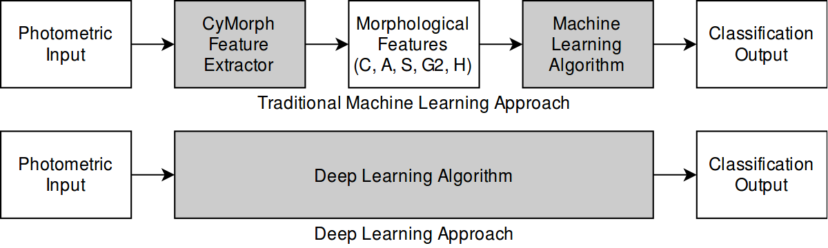
Figure 1: Illustrative sketch of traditional Machine Learning and Deep Learning flows.

The huge amount of photometric astrophysical data available and the highly increasing advancements on hardware and methods to perform automatic classifications has been leveraging related publications (Law et al., 2007; Freeman et al., 2013; Khalifa et al., 2017; Huertas-Company et al., 2018; Barchi et al., 2016; Dieleman et al., 2015; Khan et al., 2018; Huertas-Company et al., 2015; Domínguez Sánchez et al., 2018). Highlight to Domínguez Sánchez et al. (2018) who use questions and answers from Galaxy Zoo 2 for replicating the answers from the users, and provide morphology classification by T-Type in their final catalog.

The approach used in this paper is different from the one used in Domínguez Sánchez et al. (2018). Instead of using questions and answers from Galaxy Zoo 2, we use the classifications and images themselves. Also, we revisit issues not touched upon in previous studies dealing with morphological parameters (Abraham et al., 1996; Conselice et al., 2000; Conselice, 2003; Lotz et al., 2004); namely, threshold dependence in the use of the segmented image. We study the impact of that on the parameters that ultimately will be used in the TML approach.

Although it is already a well-established observation that for perception tasks (which galaxy morphology is) Deep Learning is likely to outperform machine learning models trained on hand engineered features (Russakovsky et al., 2015), this subject is in its infancy in galaxy morphology and such comparison of these two approaches have never been presented in the same work in the literature. Also, deep learning methods need huge amounts of data to learn from and huge computational resources to make it effective. Deep learning models can be hard to tune and tame, and the prediction time can take much longer than other models because of the complexity (Goodfellow et al., 2016). The traditional machine learning approach is still relevant.

This document is organized as follows: Section 2 describes the sample and data used to measure morphology and build the classification models. Section 3 describes the advances in non-parametric galaxy morphological system (CyMorph). Sections 4 and 5 describe the basics and methodology of TML and DL employed, respectively. Section 6 presents the results and validation for all experiments conducted. We compare the final product of this work with state-of-the-art catalogs in Section 7, followed by a summary in Section 8. We present catalog details in A.

2 Sample and Data

This work uses data acquired from the SDSS-DR7 (Eisenstein et al., 2011) and Galaxy Zoo catalogs (Lintott et al., 2008, 2011; Willett et al., 2013) for measuring morphology and training the classification models. The samples are composed of galaxies in r-band from SDSS-DR7 in the redshift range $0.03<z<0.1$, Petrosian magnitude in r-band brighter than 17.78 (spectroscopic magnitude limit), and $|b|\geq 30^{o}$, where $b$ is the galactic latitude.

For supervised learning purposes, we consider the defined classification from Galaxy Zoo 1 (Lintott et al., 2008, 2011, GZ1 hereafter) between E and S galaxies, and the classification from Galaxy Zoo 2 (Willett et al., 2013, GZ2) with prefixes in one of 11 following classes: Er, Ei, Ec, Sa, Sb, Sc, Sd, SBa, SBc, SBd. Other three different scenarios are explored with GZ2 supervision. Classification considering 9 classes (same as 11 classes except that we have one class for all elliptical galaxies united), 7 classes (same as previous but disconsidering the faintest galaxy types: Sd and SBd) and three classes: E, S and SB.

We study the impact of different datasets on the training process, varying the number and size of objects in the samples. We define a parameter $K$ as the area of the galaxy’s Petrosian ellipse divided by the area of the Full Width at Half Maximum (FWHM). Equation 1 presents how to calculate $K$, where $R_{P}$ is the Petrosian radius (see Petrosian, 1976; Eisenstein et al., 2011, for more details about $R_{P}$). By restricting the samples to a minimum $K$, we limit the number and size of objects in the dataset. The number of galaxies for the three main samples we explore ($K\geq$ 5, $K\geq$ 10 and $K\geq$ 20) are presented in Table 1.

$$K=\left(\frac{R_{P}}{\textnormal{FWHM}/2}\right)^{2}$$ (1)

Table 1: Number of galaxies for the main samples in this work from each database (SDSS, GZ1 and GZ2).

Restriction	Number of galaxies in
	SDSS	GZ1	GZ2
$K\geq 5$	239,833	104,787	138,430
$K\geq 10$	175,167	89,829	110,163
$K\geq 20$	96,787	58,030	67,637

With smaller values of $K$ we have more but smaller objects, while samples restricted by bigger values of $K$ have less but bigger objects. To properly check the impact of the number and sizes of objects in the samples, we explore the Deep Learning approach for three classes problem in detail with other restrictions: $K\geq$ 7, $K\geq$ 9, $K\geq$ 11, $K\geq$ 14 and $K\geq$ 17.

For Machine and Deep Learning experiments, we split the datasets from GZ1 e GZ2 into training-validation-test subsets in the proportion 80-10-10. In all experiments, each of these subsets are constrained to the same restriction (the model trained and validated with a subset restricted to $K\geq 20$ is also tested with the subset restricted to $K\geq 20$). We should keep in mind that the data used in this work, SDSS-DR7, does not have a proper spatial resolution (0.396 $\operatorname{arcsec}$ pixel ^-1) and not adequate PSF FWHM ($\sim$1.5 $\operatorname{arcsec}$). For comparison, the Dark Energy Survey (Collaboration et al., 2016, DES), has a pixel size of (0.27 $\operatorname{arcsec}$) and PSF FWHM of $\sim$0.9. This is why we study the quality of our classification as a function of $K$.

3 Advances in Non-Parametric Galaxy Morphology - CyMorph

Methodologies for computing non-parametric morphological metrics have been presented by several authors (Morgan and Mayall, 1957; Kent, 1985; Abraham et al., 1996; Takamiya, 1999; Conselice, 2003; Lotz et al., 2004; Ferrari et al., 2015; Rosa et al., 2018). In this section, we present CyMorph - a non-parametric galaxy morphology system which determines Concentration (C), Asymmetry (A), Smoothness (S), Entropy (H) and Gradient Pattern Analysis (GPA) metrics.

We perform image preprocessing techniques to ensure consistency and improve feature extraction. CyMorph achieves this goal in three major steps: producing the galaxy stamp, removing secondary objects, and generating the segmented image. To remove secondary objects inside the stamp we replace their pixels by the median value of the isophotal level that cross that object.

Concentration is the only metric we calculate using the clean galaxy stamp since we want the whole accumulated flux profile of the galaxy. For all other metrics, we use the segmented image as input which we obtain by applying a mask upon the clean image. The mask is computed by a region growing algorithm (Pedrini and Schwartz, 2007). We summarize CyMorph metrics as follows:

• Concentration is defined as $C=log_{10}(R_{1}/R_{2})$, where $R_{1}$ and $R_{2}$ are the outer and inner radii, respectively, enclosing some fraction of the total flux (Conselice, 2003; Lotz et al., 2004; Ferrari et al., 2015). We use an optimization process for setting up the best configuration parameters for CyMorph (described in Subsection 3.2). The best configuration by this method is: $C=log_{10}\left(R_{75\%}/R_{35\%}\right)$.

• Asymmetry is measured using the correlation between the original and rotated image: $A=1-s(I^{0},I^{\pi})$, where $I^{0}$ and $I^{\pi}$ are the original and the $\pi$-rotated images. The function $s()$ is the Spearman’s rank correlation coefficient (Press, 2005), which has been proved to be a stable and robust correlation coefficient (Sautter, 2018).

• Smoothness describes the flux dispersion of an image, namely how the gradient varies over the entire image. This can be measured as the correlation between the original image and its smoothed counterpart (Abraham et al., 1996; Conselice, 2003; Ferrari et al., 2015). We apply the Butterworth filter for smoothing the images. This filter provides the advantage of a continuous adaptive control of the smoothing degree applied to the image (see Kaszynski and Piskorowski, 2006; Pedrini and Schwartz, 2007; Sautter, 2018, for more details). We use the the Spearman’s rank correlation coefficient to compute smoothness, following the same reasoning as for asymmetry. We define smoothness as $S=1-s(I^{0},I^{s})$, where $I^{0}$ is the flux intensity of the original image, and $I^{s}$ is the flux intensity of the smoothed image.

• Gradient Pattern Analysis (GPA) is a well-established method to estimate the local gradient properties of a set of points, which is generally represented in a two-dimensional (2D) space (Rosa et al., 1999; Ramos et al., 2000; Rosa et al., 2003). We use the improved version of GPA developed for galaxy morphology (see Rosa et al. (2018) and references therein for more details).

• In digital image processing, the entropy of information, H, (Shannon entropy, Bishop, 2006) measures the distribution of pixel values in the image. In galaxy morphology, we expect high values of H for clumpy galaxies because of their heterogeneous pixel distribution, and low H for smooth galaxies Ferrari et al. (see 2015, for more details); Bishop (see 2006, for more details).

For more specific details about how to compute each of these metrics, see Sautter (2018) and references therein.

3.1 Geometric Histogram Separation ($\delta_{\rm{GHS}}$)

For a given sample of galaxies, CyMorph measures C, A, S, H and GPA and these parameters depend on some quantities. Our main goal is to choose the best quantities possible for reaching a maximum performance in classifying galaxies. Using an independent morphological classification (from GZ1, e.g.), we have elliptical and spiral distributions for each parameter. All we need is a simple and reliable method to objectively assign a value for the separation between elliptical and spiral distributions. Here, we measure the geometric distance between the distributions with the GHS (Geometric Histogram Separation) algorithm (see Sautter and Barchi, 2017; Rosa et al., 2018, for more details).

3.2 Optimizing Morphological Metrics Configuration

Table 2: Parameter ranges explored in the optimization process. Asymmetry is ommited since it depends only on $d_{\sigma}$. Concentration(*) does not depend on $d_{\sigma}$.

Sextractor	C*	S	G2	H
$0.1\leq d_{\sigma}\leq 5.0$	$0.55\leq R_{1}\leq 0.80$ $0.20\leq R_{2}\leq 0.45$	$0.2\leq c\leq 0.8$	$0.00\leq m_{tol}\leq 0.20$ $0.01\leq p_{tol}\leq 0.04$	$100\leq\beta\leq 250$

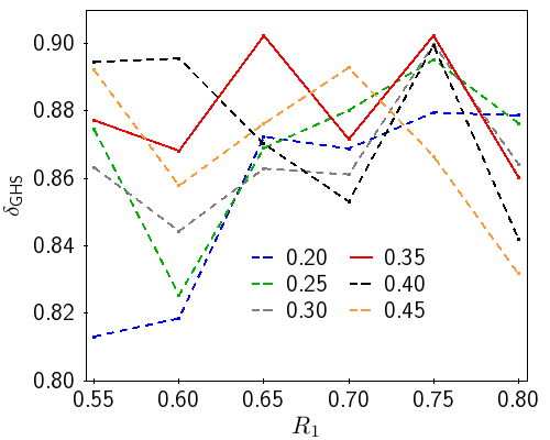
(a) Concentration

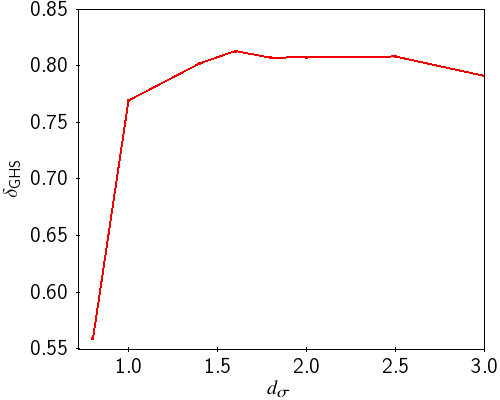
(b) Asymmetry

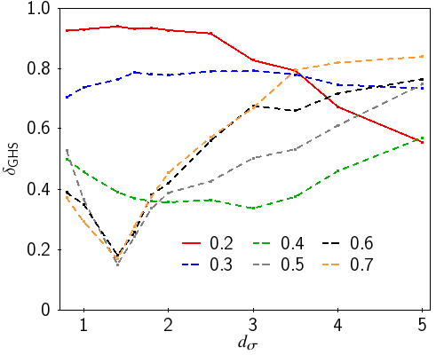
(c) Smoothness

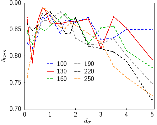
(d) Entropy

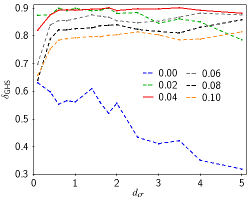
(e) GPA – modular tolerance

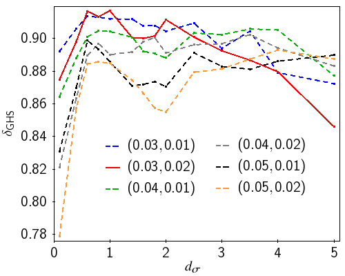
(f) GPA – fine tuning

Figure 2: Plots describing the whole optimization process for morphological metrics configuration. Red continuous lines (not dashed) have the best configuration for the given parameter. See the explanation for the experiments and best configuration results obtained in this Subsection 3.2.

CyMorph has configurable parameters that we have to fine tune for better distinction between different morphological types. One specific configuration is the threshold parameter used in Sextractor (Bertin and Arnouts, 1996) to detect objects on an image: DETECT_THRESH (hereafter $d_{\sigma}$). Sextractor detects an object if a group of connected pixels is above the background by a given $d_{\sigma}$. Thus, we want to find the minimum $d_{\sigma}$ value, sufficiently above the background limit, for which we do not lose information when computing each metric. Most of the configurable parameters are related to each morphological metric. It is important to stress these possibilities to obtain the best performance out of CyMorph. Asymmetry only depends on $d_{\sigma}$. For the other metrics, we exhaustively explore the combinations of configurable parameters: outer ($R_{1}$) and inner ($R_{2}$) radii for Concentration; control parameter $c$ of Butterworth Filter for Smoothness; modular ($m_{tol}$) and phase tolerance ($p_{tol}$) for G₂; and, number of bins $\beta$ for Entropy. Table 2 summarizes parameters and ranges explored. The optimization process may be approached in different ways. One of them consists of optimizing all variables at once by maximizing a metric which is output from the application of a local two-sample test (Kim et al., 2019). In this work, we focus on a variable-by-variable optimization which not only enables to select the best configuration and input metrics to TML methods but also leaves to the same accuracy in morphology as that obtained in GZ1 (see Section 6). In the optimization experiments reported here, we randomly select a sample with 1,000 ellipticals and 1,000 spiral galaxies. Figure 2 presents the results for all optimization experiments. In each plot, all lines are dashed except the red one which contains the best configuration for a given metric. The y-axis has GHS separation values ($\delta_{\rm{GHS}}$) in every panel. In the following Subsection, we interpret the results displayed in Figure 2.

3.3 Results on Morphology

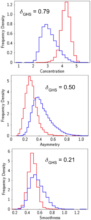
Figure 3: Results on galaxy morphology using Classic CAS (Conselice, 2003; Lotz et al., 2004), with elliptical galaxies in red and spiral galaxies in blue.

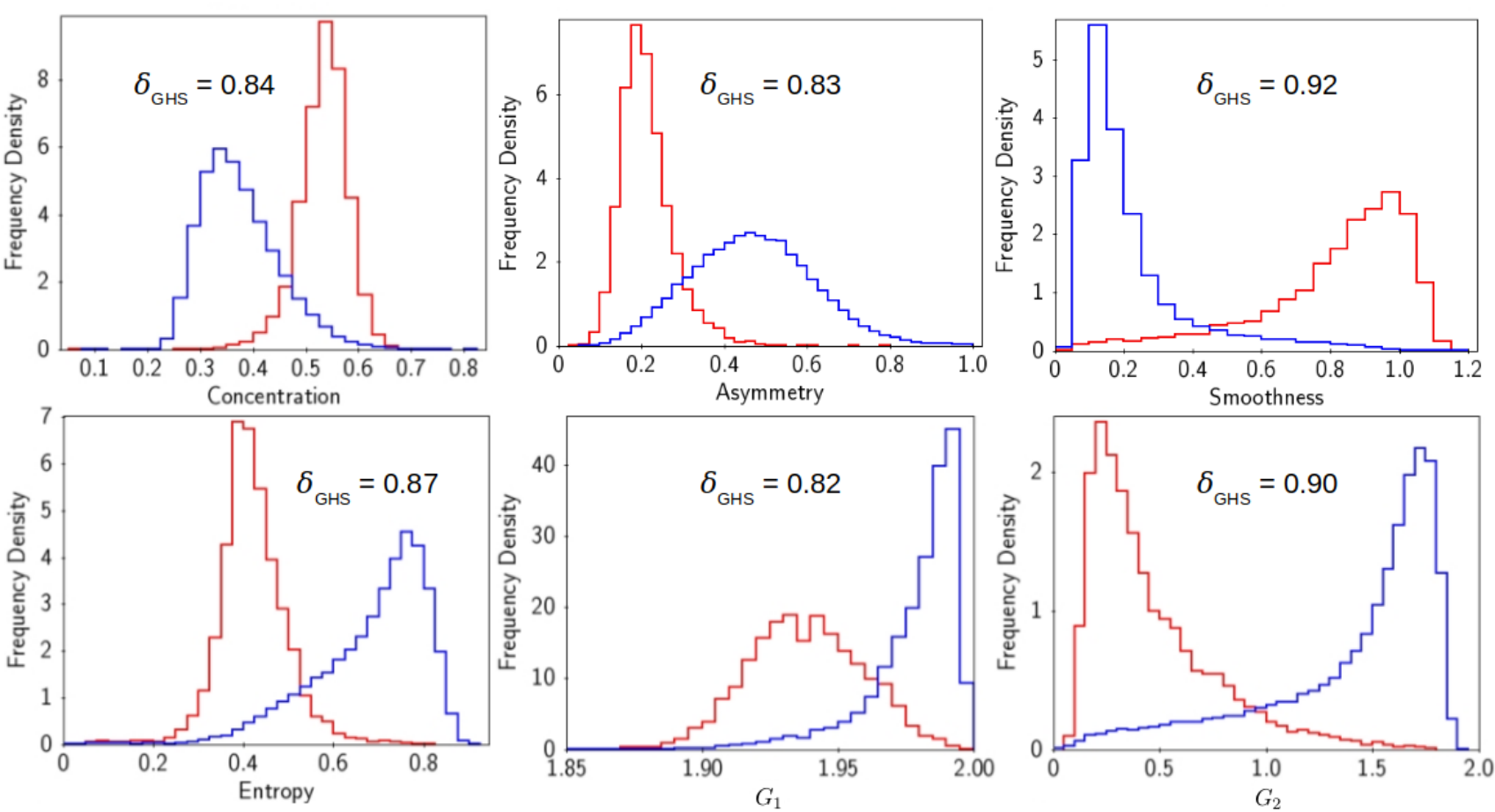
Figure 4: Results on galaxy morphology using CyMorph (the proposed system), with elliptical galaxies in red and spiral galaxies in blue.

In this subsection, we compare the results obtained by computing the classic CAS system (Conselice, 2003; Lotz et al., 2004), which are presented in Figure 3 and the optimal results obtained by CyMorph system, exhibited in (Figure 4). Conselice (2003); Lotz et al. (2004) estimate Concentration and Asymmetry without significant differences among them. However, Smoothness is implemented in different ways. We present Smoothness as in Lotz et al. (2004), which gives the most consistent results. For each non-parametric morphological index, we display a binomial distribution histogram with elliptical galaxies (in red) and spiral galaxies (in blue). In each panel we also list the $\delta_{\rm{GHS}}$ value.

The classic CAS system has the best result with Concentration ($\delta_{\rm{GHS}}=0.79$), however, this is still lower than the lowest performance obtained by CyMorph metrics, which is Asymmetry with $\delta_{\rm{GHS}}=0.83$ (see Figure 4). With this improvement in CAS metrics within CyMorph (Smoothness, for instance, the best result: $\delta_{\rm{GHS}}=0.92$), and the adoption of Entropy ($\delta_{\rm{GHS}}=0.87$) and Gradient Pattern Analysis ($G_{2}$: $\delta_{\rm{GHS}}=0.90$), we have satisfactory non-parametric morphology metrics to serve as input features to the Traditional Machine Learning algorithms. $G_{2}$ and $H$, two of the best metrics by $\delta_{\rm{GHS}}$, have highly correlated results: the greater the Entropy value, the more asymmetric gradient patters, and vice versa, lower entropy values correspond to more symmetric gradient patters.

The reasons for the improvement upon classic metrics can be summarized as: (1) the three-step preprocessing, (2) Butterworth filter to smooth the image (concerning Smoothness metric), (3) usage of correlation coefficients for Asymmetry and Smoothness, and (4) optimization process to better configure each metric.

4 Machine Learning Applied to Galaxy Morphology

CyMorph presents a consistent non-parametric morphological system. By employing Machine Learning (ML) methods with CyMorph metrics as features, we can value the best morphological information and obtain reliable and consistent classification results in galaxy morphology. An alternative would be to test logistic regression and other regression methods, which is beyond the scope of this paper. The five input features for the learning process are the best morphological metrics (given by $\delta_{\rm{GHS}}$) computed by CyMorph: C, A, S, G₂ and H. We maintain the restriction related to the area of the galaxies to build up different classification models: (1) $K\geq 5$; (2) $K\geq 10$; and (3) $K\geq 20$, i.e., the area of the galaxy is at least five (model 1), ten (model 2) and twenty (model 3) times larger than the FWHM area for each corresponding object, respectively.

We build up Decision Tree (DT), Support Vector Machine (SVM) and Multilayer Perceptron (MLP) models to classify galaxies considering different numbers of classes. We use scikit-learn (Pedregosa et al., 2011) python library to perform the experiments and procedures reported in this Section. We use Cross-Validation (CV) to split the dataset in training-validation-testing to address the trade-off between bias and variance Mitchell (1997); Géron (2019). First, we split the dataset in a 90/10 proportion for training and testing sets, respectively. CV is applied in the 90% portion of the dataset.

Consistent performance validation metrics are crucial to guide the learning process and to objectively measure the performance of each model. No metric is designed to perform this task alone. We employ the Overall Accuracy (OA) as the figure of merit to compare all the different models. Additionally, we employ other performance metrics: Precision (P) and Recall (R) – see Mitchell (1997); Géron (2019); Goodfellow et al. (2016) for more details about OA, P, and R. For a further analysis on the problem with two classes, we use the Receiver Operating Characteristic (ROC) curve and the Area Under the ROC curve (AUC, Bradley, 1997).

One of the most used methods for classification and regression is the Decision Tree (DT). Among the different versions and variations of DTs, we use the optimized version of Classification and Regression Tree (CART) algorithm. CART builds up binary trees using feature and threshold that yield the largest information gain at each node (Quinlan, 1986; Géron, 2019).

Another influential method for supervised classification is the Support Vector Machine (SVM) which finds the optimal hyperplane that divides the target classes. SVM performs this task by drawing infinite different hyperplanes for separating target classes aiming to get the minimum error rate (Hearst et al., 1998; Cortes and Vapnik, 1995).

A standard Neural Network (NN) consists of many simple, connected neurons, each one being a computing unit which outputs a sequence of real-valued activations. Neurons are organized in layers: input, hidden (which may be one or many) and output. A Multilayer Perceptron (MLP) has at least three layers (one input, one hidden and one output layer). Each neuron has $n$ inputs $i$, weights ($w$), bias ($b$), an activation function ($F(x)$) and output ($y$) (see Mitchell, 1997; Géron, 2019; Goodfellow et al., 2016, for more details about NN). We define the MLP architecture by empirically testing different configurations for the two classes problem using the restricted sample defined by $K\geq 20$. We predefine three hidden layers, test different numbers of neurons and alternate between logistic and ReLU as activation functions. Our final NN configuration consists of 44 neurons in the first, 88 in the second and 22 in the third hidden layer, with ReLu as the activation function.

5 Deep Learning

A Neural Network (NN) can be extremely complex when using an architecture with many layers. Deep Learning (DL) methods are built through a deep neural network with multiple layers of non-linear transformations. Deep Convolutional Neural Network (CNN) or simply Convolutional Networks (Lecun, 1989) are a special kind of neural network for processing data with grid-like topology. Convolution preserves the spatial relationship between pixels by using submatrices from the input data to learn features. It is not feasible to go through all the possibilities of architectures and configurations concerning CNNs. In this work, we perform different experiments focusing on two notable robust CNN architectures, Residual Networks (ResNet, He et al., 2016) and GoogleNet (Szegedy et al., 2015), judging overall accuracy performance and training time. We select the architecture which provide the best overall results: GoogleNet Inception, the winner of ILSVRC 2014 Classification Challenge in visual databases (see Szegedy et al., 2015; Géron, 2019, for more details).

6 Results on Classification and Discussion

6.1 Classifier's performance by Overall Accuracy (OA)

Table 3: Overall Accuracy (OA in percentage) for all approaches considering GZ1 classification (elliptical and spiral galaxies separation).

	$K\geq 5$				$K\geq 10$				$K\geq 20$
	DT	SVM	MLP	CNN	DT	SVM	MLP	CNN	DT	SVM	MLP	CNN
two classes	94.8	94.6	94.6	98.7	95.7	95.8	95.6	99.1	98.5	98.6	98.6	99.5

Table 4: Overall Accuracy (OA in percentage) for all approaches considering GZ2 classification. The darker the green colour of a cell, the better OA obtained.

	$K\geq 5$				$K\geq 10$				$K\geq 20$
	DT	SVM	MLP	CNN	DT	SVM	MLP	CNN	DT	SVM	MLP	CNN
11 classes	49.3	48.8	49.4	63.0	51.6	51.6	51.7	63.0	57.7	57.4	57.7	65.2
9 classes	60.9	63.2	63.0	70.2	60.5	63.8	63.6	75.7	63.5	66.4	66.2	67.4
7 classes	63.0	62.5	63.3	72.2	62.9	62.6	63.0	77.6	65.9	65.8	66.0	70.0
3 classes	71.9	71.2	71.2	80.8	71.9	74.6	74.9	81.8	78.7	78.5	78.8	82.7

As we have shown in previous sections, there are several parameters driving the final classification and an appropriate figure of merit is needed to establish which setup/method works best. In Tables 3 and 4, we present the Overall Accuracy (OA) achieved by all the experiments carried-out in this work. The main goal here is to distinguish between an Early-Type Galaxy (ETG), elliptical (E), and a Late-Type Galaxy (LTG), spiral (S). In the case of TML, using the $K\geq 20$ sample, all methods reached over 98% of OA. In this training set, there are many more S galaxies ($\sim$87%) than E galaxies ($\sim$13%). This difference in the number of examples between classes is called class imbalance. We discuss class imbalance in Subsection 6.2. Despite of the imbalance, we have at least 95% precision and 96% recall for E systems. Since most of the training set is constituted by S galaxies, it is not surprising that we reach $\sim$99% precision and recall, establishing a model with $\sim$99% OA for this dataset.

Overall, CNN is the best approach to establish morphological classification of galaxies. We can safely assert that starting from the classes E and S from Galaxy Zoo 1, we can reproduce the human eye classification with all methods and samples (OA $>$ 94.5%). When trying to distinguish among 11 classes, the problem is much more complex, as it would be for the human eye, and the best result is $\rm OA\sim 65.2$% using CNN with $K\geq 20$. However, if we use only three classes we find an OA $>$ 80% with CNN, for all samples, namely elliptical (E), unbarred (S) and barred spiral (SB) galaxies. We study the three classes problem considering imbalance and different samples in Subsection 6.2.

6.2 Class Imbalance in Galaxy Morphology

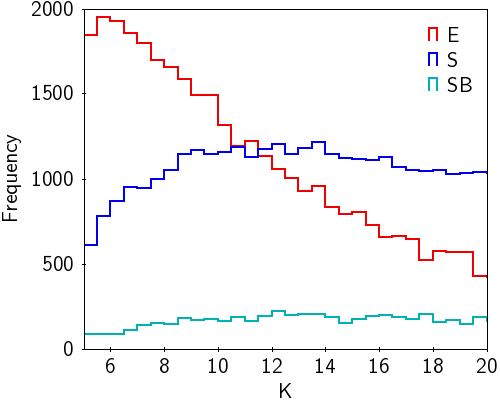
(a) Number of examples as a function of K, for different classes.

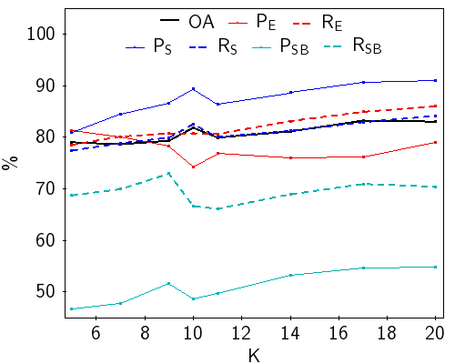
(b) Imbalanced (original dataset).

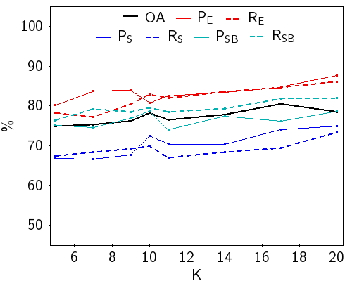
(c) Balanced – SMOTE.

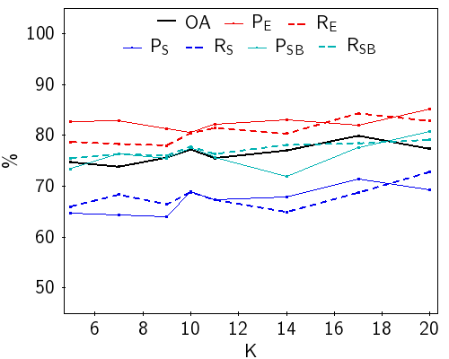
(d) Balanced – undersampling.

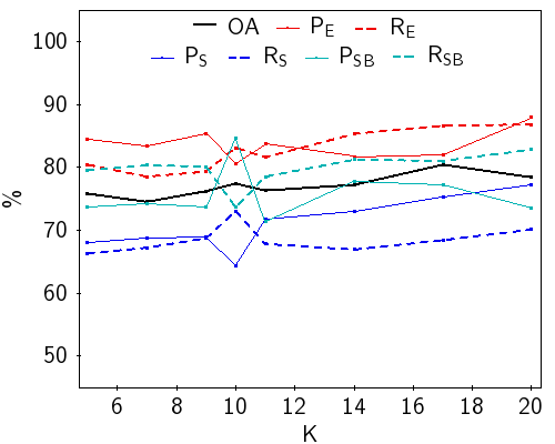
(e) Balanced – oversampling.

Figure 5: The first plot shows number of elliptical (E), unbarred spiral (S) and barred spiral (SB) galaxies from GZ2 classification varying K. The other four plots are related to the class imbalance problem considering three classes: E (in redder colours), S and SB – in bluer colours. The black lines indicate the Overall Accuracy (OA). For each of the three classes, continuos lines represent Precision (P) and the dashed lines indicate Recall (R), considering the original imbalanced dataset (panel b), the dataset generated with SMOTE (panel c), the undersampled balanced dataset (panel d) and the oversampled balanced dataset (panel e).

The class imbalance problem is one of the top in data mining, data science, and pattern recognition (Yang and Wu, 2006). It arises when at least one of the classes has considerably fewer examples than the other(s). This problem is inherent in galaxy morphology, as the number of examples among classes will never be equal. Applying the restriction of $K\geq 20$ in the dataset from Galaxy Zoo 1 (Lintott et al., 2008, 2011), for example, there are $\sim$ 87% of galaxies classified as spiral and only $\sim$13% as elliptical. Balancing the dataset generally improves the performance for minority classes (since we increase the number of examples of such classes for training), and thus increases precision and recall for these classes (Goodfellow et al., 2016). Figure 5a shows the number of examples from three classes (E, S, SB) in Galaxy Zoo 2 - SDSS DR7 in different bins of K. The bin size is 0.5 and K varies from 5 to 20. SB is the minority class with the number of galaxies approximately constant – the bar component is a feature identified in all resolutions explored. The number of S galaxies increases until $K=10$, approximately where the numbers of S and E galaxies are equal.

We investigate the impact of the imbalance class problem on the morphological classification testing four different datasets: imbalanced, undersampling, oversampling and Synthetic Minority Over-sampling Technique (SMOTE). The imbalanced dataset is the original query. In the undersampling dataset all classes have the same number of examples as SB originally have. For oversampling, we sample the minority class set with replacement. Using SMOTE, we synthetically generate more examples for SB and we consider the smaller of either the number of E galaxies or double the number of SB galaxies to be the number of examples for each class (Pedregosa et al., 2011).

Figures 5b, 5c, 5d and 5e exhibit OA, P, and R for all experiments exploring the imbalance class problem considering the three classes described above. The minority class (SB) is the one more affected by imbalanced datasets, with low P (51%) and R (69%), in average. By employing balancing techniques, we improve to P (76%) and R (79%) for the minority class, thus reducing the misclassification for the SB class. All balancing strategies have similar performances. In all strategies, there is a $\Delta\rm{OA}\sim$ 2% when $K$ varies from 5 to 20. From panels (b) to (e) of Figure 10, we notice that OA weakly increases with $K$, a trend that would imply that restricting the sample to bigger objects reduces classification problems, but the impact is not very significant. Thus, our model built up with the sample restricted by $K\geq$ 5 can safely be used to classify an unknown dataset as it classifies smaller objects with a similar OA compared to bigger objects (such as $K\geq$ 20).

In the remaining of this paper we continue analysing three methods: Traditional Machine Learning (TML) and Deep Learning (DL) approaches using imbalanced dataset for discriminating between two classes; and DL using SMOTE dataset to classify into three classes. For the TML approach, we choose the Decision Tree (DT) algorithm as it is the simplest solution (compared to Support Vector Machine and Artificial Neural Network) and the results have $\Delta\rm{OA}\sim 0$ among them (Occam’s razor, Blumer et al., 1987). For three classes, we select the model trained with SMOTE dataset because it is in the middle ground between under and overbalancing techniques, and the results using different balanced datasets are equivalent (Figures 5c, 5d and 5e). These are the selected classifiers to build up the catalog – see details about the final catalog in A.

6.3 Classifier's performance by ROC curve and AUC

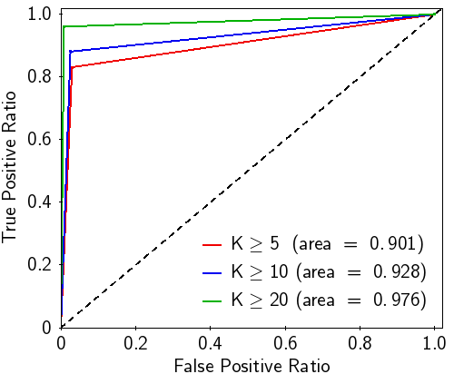
(a) ROC curves - TML - two classes.

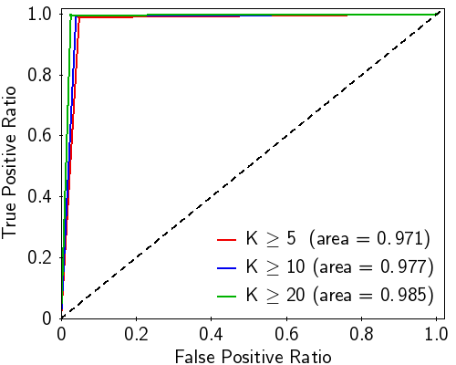
(b) ROC curves - DL - two classes.

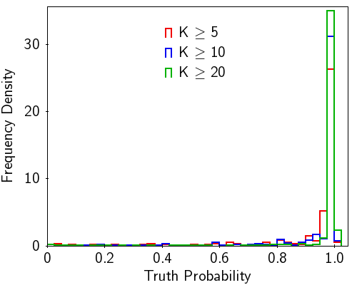
(c) Truth Probability - TML - two classes.

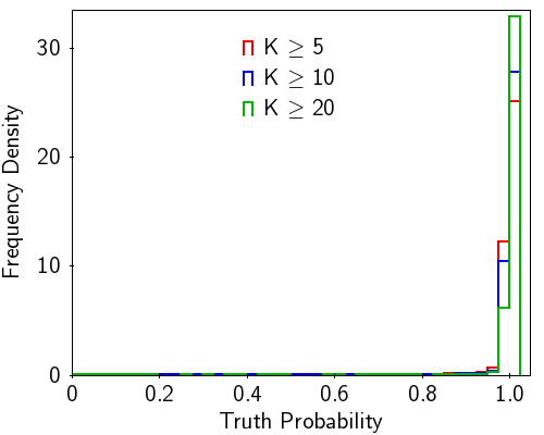
(d) Truth Probability - DL - two classes.

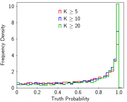
(e) Truth Probability - DL - three classes.

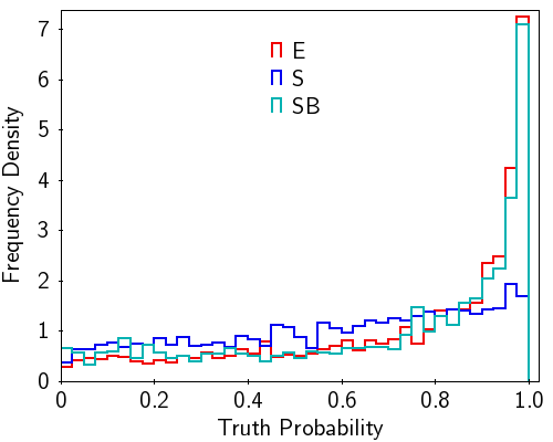
(f) Truth Probability - DL - three classes - $K\geq 5$

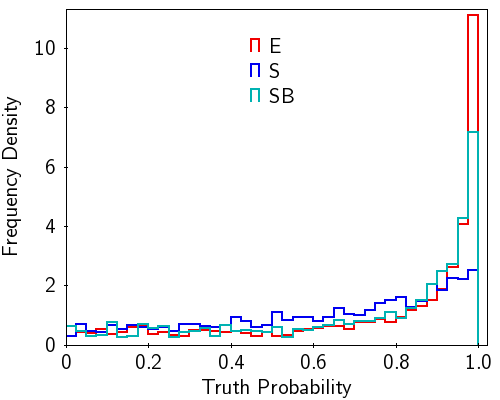
(g) Truth Probability - DL - three classes - $K\geq 10$

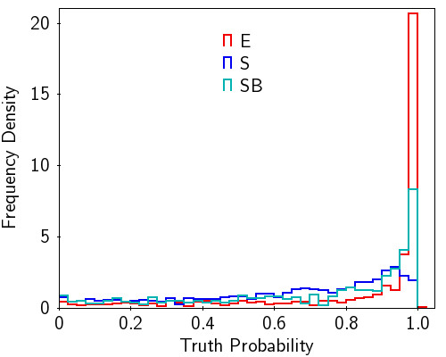
(h) Truth Probability - DL - three classes - $K\geq 20$

Figure 6: The first row presents ROC Curve and the Area Under the ROC Curve (AUC – area) for each approach and different dataset restrictions considering the two classes problem (panels a and b). Such plots consider the ground truth and predicted labels. The dotted black line represents a random guess. The second row shows histograms with ground truth probabilities given by the models for each class (panels c, d, e). The third row presents histograms with ground truth probabilities given by the models for each class in regard to the three classes problem (panels f, g, h).

One of the most important issues in machine learning is performance measurement. A very popular method is the ROC (Receiver Operating Characteristics) curve and the Area Under the ROC curve (AUC, Bradley, 1997). In our particular case, ROC is the probability curve and AUC represents a measure of separability. It indicates how a model is capable of distinguishing between classes. Higher the AUC, better the model is at predicting E’s as E’s and S’s as S’s. Based on data presented in Tables 3 and 4, Figures 6a and 6b display the ROC curves. Figures 6c, 6d and 6e show the histograms with ground truth probabilities given by the models using different datasets, and deeper into the three classes problem Figures 6f, 6g and 6h exhibit histograms with ground truth probabilities given by the models for each class.

ROC curves are typically used in binary classification to study the output of a classifier (Bradley, 1997; Géron, 2019). Figures 6a and 6b show ROC curves considering the ground truth and predicted labels (no probabilities). These ROC curves and area values confirm what Table 3 shows with OA: all models have high standards for acting upon the two classes problem with AUC $>$ 0.90; restricting to the Deep Learning (DL) approach we improve it to AUC $>$ 0.97. By experimenting with different dataset restrictions and approaches we can draw some interesting conclusions. The restriction on the dataset has more impact on TML approach than using DL. The ROC curves are closer to each other on Figure 6b ($\Delta\rm{AUC}=0.014$) than 6a ($\Delta\rm{AUC}=0.075$). One example is to compare TML using $K\geq 20$ and DL using $K\geq 10$ ($\Delta\rm{OA}\sim 0.5\%$ and $\Delta\rm{AUC}\sim 0$ among them). Using smaller objects, DL can achieve a very similar performance as TML using bigger objects.

The output probabilities given by these models with regard to the ground truth from Galaxy Zoo are explored in Figures 6c, 6d, 6e, 6f, 6g and 6h). These histograms do not distinguish each class. We consider the output probability from each model for the ground truth of each galaxy. Again, we confirm that: (1) both approaches have a very high performance considering two classes – very high concentration of frequency density for truth probability $>$ 0.9, and (2) DL (Figure 6d) improves the results when comparing to TML (Figure 6c) by reducing the frequency density with low truth probability values. The impact of the dataset restriction continues as well: the higher we set the threshold for $K$, the denser the frequency for truth probability $>$ 0.9.

Although Figure 6e also presents a high frequency density for truth probability $>0.9$, it is natural to see a higher frequency density for lower truth probabilities when comparing to Figures 6c and 6d since this problem is more complex when having one more class to consider. Exploring further, Figures 6f, 6g and 6h show different dataset restrictions employed to train models on the three classes problem. Once more, we can see clearly the impact of using bigger (but less) objects: the frequency density for lower truth probabilities decreases from Figure 6f to Figure 6g and gets even lower in Figure 6h. Non-barred spiral galaxies does not have a very high concentration for truth probability $>$ 0.9. However, the other two classes have a high frequency density for truth probability $>$ 0.9.

6.4 Learning About Differences between TML and DL From Misclassifications

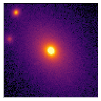
(a) 587732582054559872
GZ1: 0; TML: 1

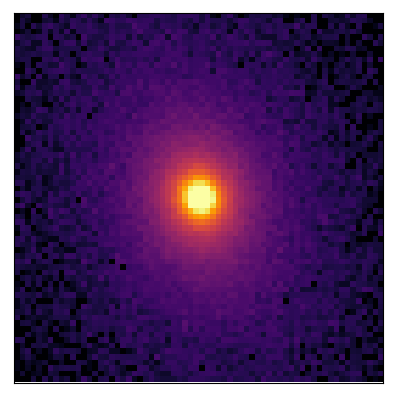
(b) 587741491440713856
GZ1: 0; TML: 1

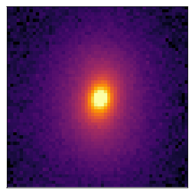
(c) 588023046942425216
GZ1: 0; TML: 1

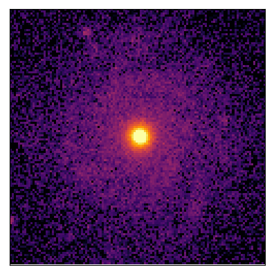
(d) 587733604255989888
GZ1: 1; TML: 0

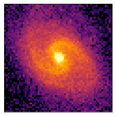
(e) 587735696448749696
GZ1: 1; TML: 0

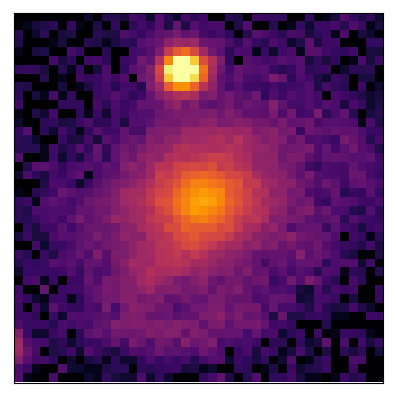
(f) 587742059994480768
GZ1: 1; TML: 0

Figure 7: Sample of misclassified galaxies comparing the classification of Galaxy Zoo 1 (GZ1) and our Traditional Machine Learning (TML) approach trained with the sample restricted by $K\geq 20$. Under each galaxy image, we present the object ID number from SDSS-DR7 and the classification given by GZ1 and TML (0: Elliptical; 1: Spiral).

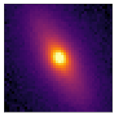
(a) 587739305287811105
GZ1: 0; DL: 1

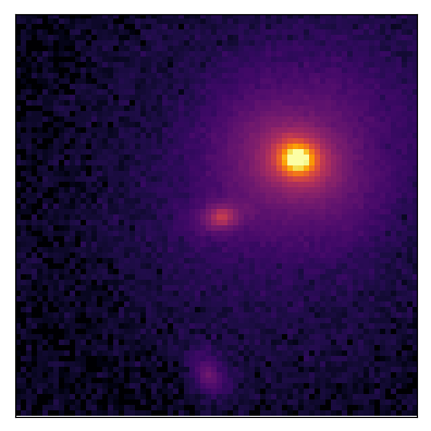
(b) 587741489822302351
GZ1: 0; DL: 1

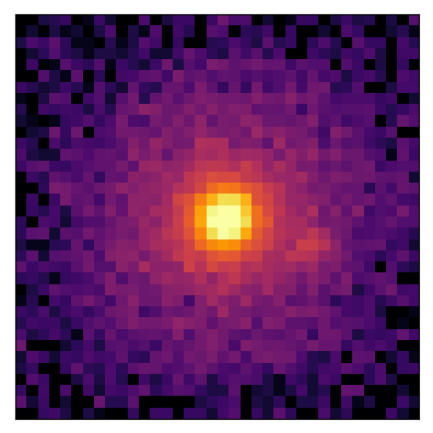
(c) 588013382210093213
GZ1: 0; DL: 1

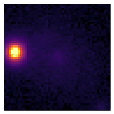
(d) 587739165702422588
GZ1: 1; DL: 0

(e) 587742576444571849
GZ1: 1; DL: 0

(f) 588017626688585921
GZ1: 1; DL: 0

Figure 8: Sample of misclassified galaxies comparing the classification of Galaxy Zoo 1 (GZ1) and our Deep Learning (DL) approach trained with the sample restricted by $K\geq 20$. Under each galaxy image, we present the object ID number from SDSS-DR7 and the classification given by GZ1 and DL (0: Elliptical; 1: Spiral).

The two approaches used in this work, Traditional Machine Learning – TML; and Deep Learning – DL, achieve almost the ideal performance considering the Overall Accuracy (OA $\sim$ 99%) for the two classes problem with the sample restricted by $K\geq 20$. However, it is still worthwhile to further investigate what causes misclassification even at a low percentage. We remind the reader that misclassification is always established using Galaxy Zoo 1 as the ground truth. Figure 7 presents some examples of misclassification using TML. In the first and the last image we see that the preprocessing phase was not able to properly clean the image or discard such examples as bright objects remain close to the central galaxy. The other cases reflect the variance in the parameters used by Decision Tree and the natural uncertainty of the process. In Figure 8 we display some misclassified galaxies by DL. Here, the absence of preprocessing allows galaxies to be too close to the border (second and fourth images) and as before the other examples are simple misclassifications imposed by the method itself, namely the galaxies are easy to be misclassified – a bright central structure which gradually fades away to the outer part of the galaxy, which, in a more detailed classification (visual), could be considered as a S0 galaxy. We should stress that this misclassification is very low. Using a sample of 6,763 galaxies selected from the grand total of 58,030 galaxies listed in Table 1 ( $K\geq 20$, from GZ1), not used in the training process, TML misclassifies only 72 galaxies (1%) while DL gets 0.5% misclassified galaxies. Also, we noticed that none of the galaxies misclassified by TML are in the list of misclassifications by DL. These results seem innocuous, however they remind us of how important is to treat objects close to the border and those near a very bright source as an specific set since this will always be present in any sample. It also reinforces how important it is that we treat independent methodologies along the process of establishing a final morphology attached to an object. The examples presented here show how visual inspection is still an important source of learning about morphology (the problem is not the eye but the quality of the image placed in front of you), although inefficient for large catalogs currently available and the ones coming up in the near future.

6.5 Validating Classification with Spectroscopic Data

The performance analysis presented in the previous section reflects our ability to establish a morphological classification using a given method among several that might in principle works properly, and that’s why finding a robust figure of merit is of paramount importance. However, an independent validation is even more essential when presenting a catalog with reliable morphology, namely, we have to show that our new classes recover well know relations. Figure 9 presents histograms of Age, stellar mass (M_stellar), Metallicity ([Z/H]) and central velocity dispersion ($\sigma$) (for more details on how these parameters were obtained and errors, see de Carvalho et al., 2017). In every panel we show the distribution for ellipticals (in red) and spirals (in blue). Also, we display the parameter $\delta_{\rm GHS}$ which measures how distant these two distributions are (see Section 3.8). This validation procedure was done using only galaxies from GZ1 classified as ”Undefined”. The classification here is provided by DT (TML). We remind an important characteristic of the samples: $K\geq 5$, which has more but smaller objects; $K\geq 10$; and $K\geq 20$, which has less but bigger objects. Although we have a bigger dataset with $K\geq 5$, the presence of smaller objects impairs our classification. The degradation of the quality of our classification as we go to smaller galaxies in evident from Figure 9 where $\delta_{\rm GHS}$ decreases for smaller $K$ for all quantities except for Age where only a small fluctuation is noticed.

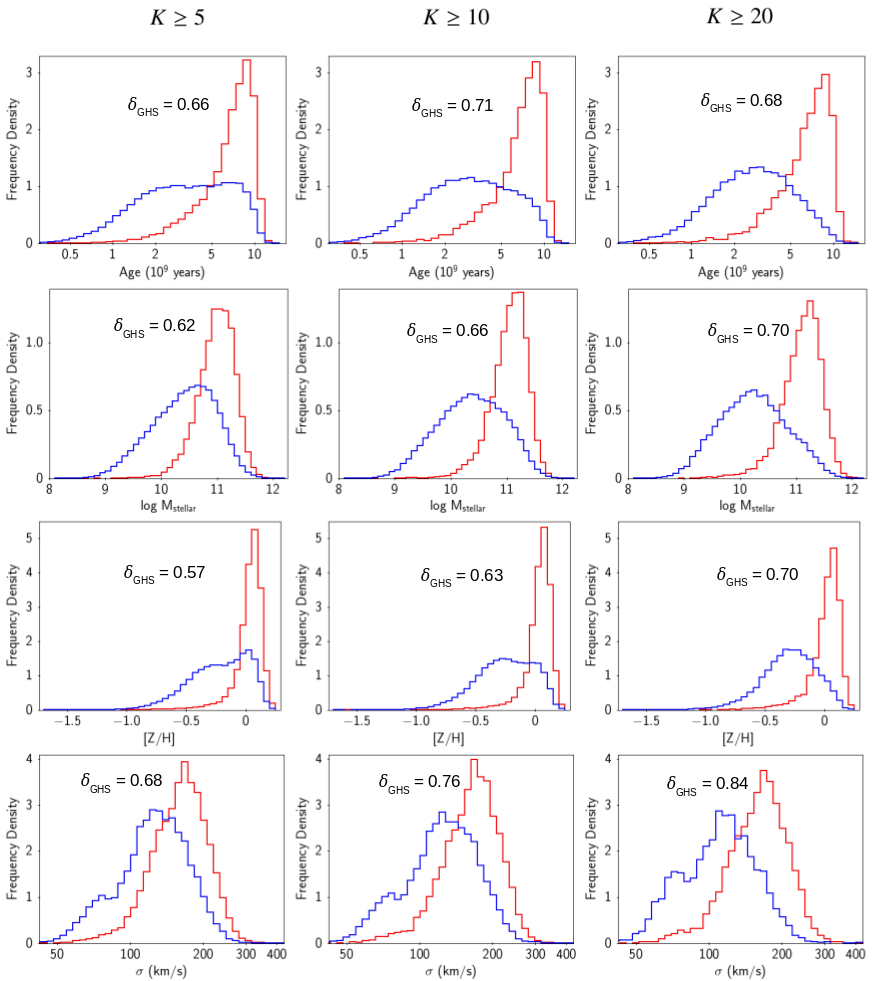
Figure 9: Spectroscopic validation for the “Undefined” galaxies from Galaxy Zoo 1 which here are classified by our Machine Learning approach using Decision Tree. Elliptical galaxies are displayed in red and spirals in blue. In each panel we give the geometric histogram separation, $\delta_{\rm GHS}$.

The number of galaxies for each histogram from Figure 9 is as follows:

• $K\geq 5$: 13,373 ellipticals; 87,095 spirals; Total: 100,468.

• $K\geq 10$: 9,030 ellipticals; 59,096 spirals; Total: 68,126.

• $K\geq 20$: 6,390 ellipticals; 24,988 spirals; Total: 31,378.

Figure 9 shows how our classification recovers well known properties of galaxies like in the first row we see that ellipticals have ages peaked around 9 Gyr while spirals are younger and the distributions is more spread, probably due to the contamination by S0 galaxies. The second row exhibits the stellar mass distribution and again ellipticals have larger M_stellar compared to spirals with a difference of $\sim$0.9 dex, peak to peak. In the third row it is also evident the difference in metallicity ($\sim$0.4 dex), ellipticals are more metal rich than spirals, specially for larger systems. Finally, the distributions of central velocity dispersion show larger values for ellipticals and for spirals we even see a bimodality which reflects the disk to bulge ratio in this morphological type. These distributions attest credibility to our final classification using DT (TML).

6.6 Case Study: Star Formation Acceleration and Morphologies

In this section we describe an application of the method presented here to study the relation between morphologies and galaxy evolution. More specifically, we use the method to classify a sample of galaxies between disks and spirals and measure quenching timescales for each group separately. There results will be discussed in detail in Sá-Freitas et al. (in prep).

It has been established that galaxies are show a bimodal distribution in colors, with two distinct peaks with young (blue) and old (red) stellar populations (e.g., Baldry et al., 2004; Wyder et al., 2007) and a minimum in the distribution commonly known as the green valley. Although it is generally accepted that galaxies move from blue to red, the physical processes associated with this transition are not completely understood, i.e., we do not know which phenomena are responsible for accelerating the decline in star formation rates, whether a single one or a combination of effects.

Using galaxy colours and stellar population synthesis models, Schawinski et al. (2014) has shown that galaxy quenching can be divided into two distinct processes depending on morphology: elliptical galaxies quench faster, probably through merger activity. Nogueira-Cavalcante et al. (2018) have reached a similar conclusion with more precise measurements from spectral indices (the 4000Å break in the spectral continuum and the equivalent width of the $H_{\delta}$ absorption line). Nevertheless, both these works rely on assuming specific exponentially declining star-formation histories.

To circumvent this limitation, Martin et al. (2017) have developed a method using the same spectral indices but with no restraints regarding a parametric star formation history. The authors have shown, by comparisons with results from cosmological simulations, that one could infer the instantaneous time derivative of the star-formation rates, denominated the star-formation acceleration. Formally, this is defined as

$$SFA\equiv\frac{d}{dt}({\rm NUV}-{\rm r}),$$ (2)

with higher values representing stronger quenching.

In Sá-Freitas et al. (in prep) we apply this methodology to a sample of galaxies out to $z=0.120$, divided by morphology. We only consider galaxies brighter than $M_{r}=-20.4$ for the sake of sample completeness. When compared to previous works, we are able to measure SFA in galaxies according to morphology for all objects, regardless of colour and assumed quenching histories. In that sense, the learning techniques presented here are fundamental to our analysis: by classifying a much larger number of galaxies (almost 30,000 galaxies in total), we are able to bin our sample by colours and draw conclusions based on smaller subsamples of objects according to their morphologies.

In Figure 10 we show our results: as expected, the bluest galaxies are currently undergoing strong bursts, while red galaxies are typically quenching. More importantly, we detect a significant distinction between SFA values for spirals and ellipticals in the green valley. Elliptical galaxies are quenching more strongly, while spirals appear to be moving gradually towards redder colours. We perform Kolmogorov-Smirnoff and Anderson-Darling tests to test for the null hypothesis that the distributions for spirals and ellipticals are drawn from the same parent sample in each bin, ruling this out ($p<0.05$) only for $2\lesssim({\rm NUV}-{\rm r})\lesssim 5$. We therefore conclude that this is an effect distinguishable primarily within the green valley, which means that the star formation histories of spirals and ellipticals are only significantly different during their transition to the red sequence.

In the near future, we expect the large upcoming imaging and spectroscopic surveys such as Euclid and DESI to increase our samples significantly, and deep learning techniques will yield reliable morphological classification of millions of objects. This will in turn allow us to further divide our galaxy sample, correlating morphologies with other phenomena such as AGN activity and environment in order to narrow our studies to the specific impact of each on the star formation histories of spiral and elliptical galaxies.

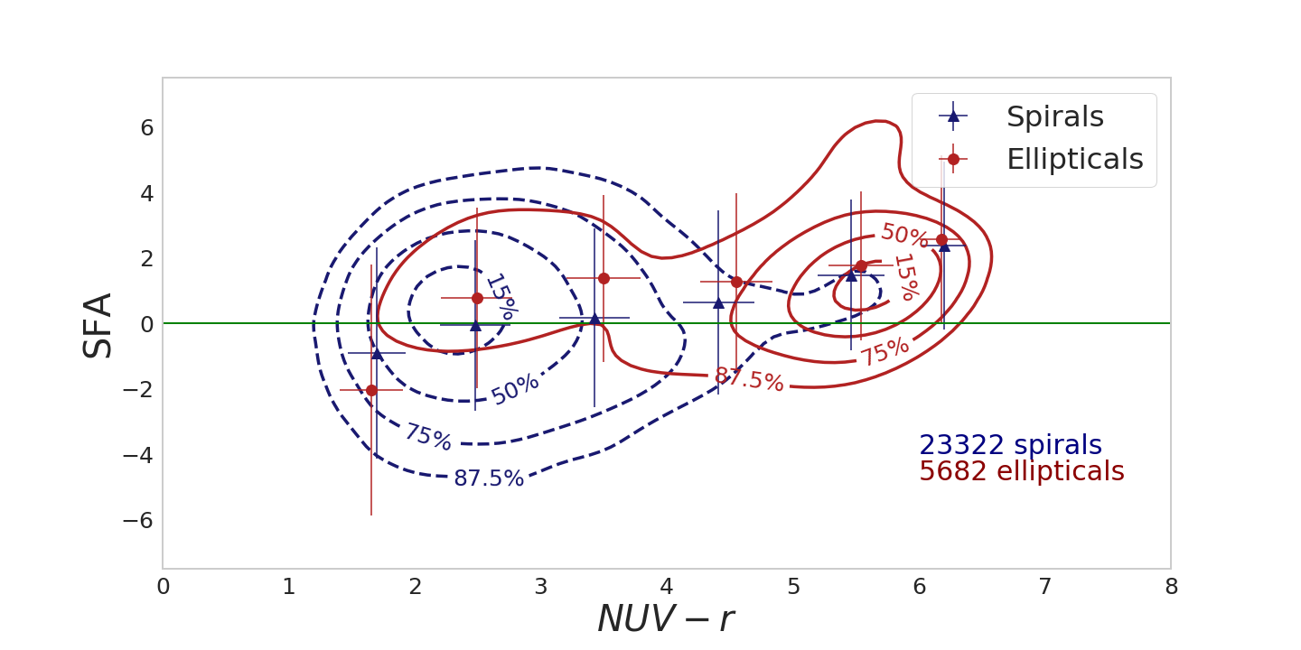
Figure 10: Star formation acceleration (SFA) as a function of NUV-r colours. Higher SFA values represent faster quenching, while more negative values indicate strong bursts of star formation, with the green line showing no current variation in SFR. Data are binned in colour, with blue triangles for spiral galaxies and red circles for ellipticals. Error bars show the standard deviation within each bin. Contours show the number of galaxies in the diagram as percentage of the total count for each morphological type. Red galaxies are statistically indistinguishable, while ellipticals in the green valley are quenching significantly faster than spirals. At the blue end, the difference is not large enough for this sample to draw any conclusions.

7 Comparison to Other Available Catalogs

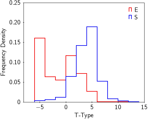
(a) Traditional Machine Learning - two classes.

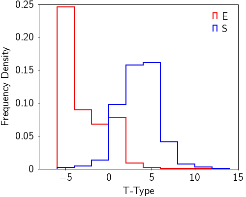
(b) CNN - two classes.

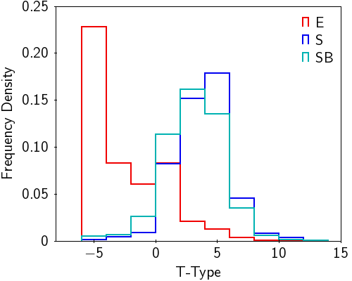
(c) CNN - three classes.

Figure 11: Histograms (normalized by area) presenting classifications for Nair and Abraham (2010) sample by T-Type using Traditional Machine Learning classification with two classes (panel a) and classification with two (panel b) and three classes (panel c) from deep CNN.

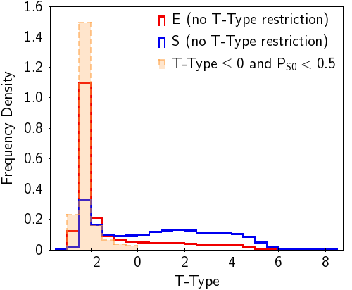
(a) Traditional Machine Learning - two classes.

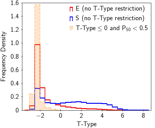
(b) CNN - two classes.

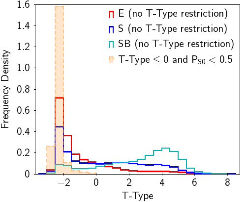
(c) CNN - three classes.

Figure 12: Histograms presenting classifications for Domínguez Sánchez et al. (2018) sample by T-Type using Traditional Machine Learning classification with two classes (panel a), and, classification with two (panel b) and three classes (panel c) from deep CNN (normalized by area).

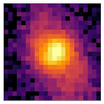
(a) 587742903942840576

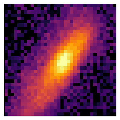
(b) 587745244699623552

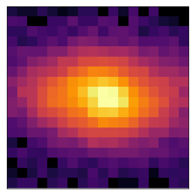
(c) 588007004732719488

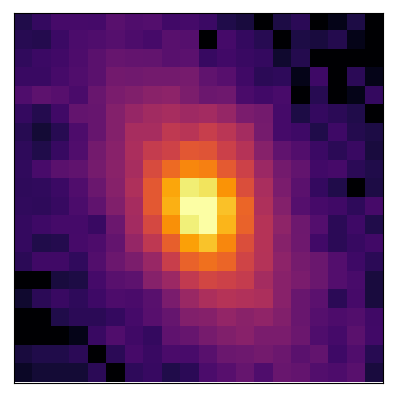
(d) 588007005231776000

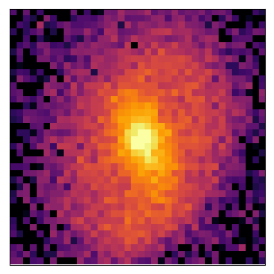
(e) 588007005239050496

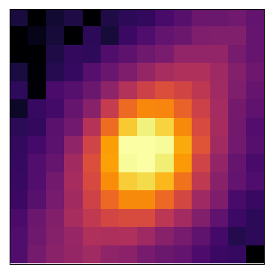
(f) 588009367478403200

Figure 13: Sample classified as spiral galaxies by our classifier with -2.25 $\leq$ T-Type $\leq$ -2 by Domínguez Sánchez et al. (2018). The object ID number from SDSS-DR7 is presented under each galaxy image.

To attest the reliability of the morphological classification we provide in this work (see A for details about our catalog), it is of paramount importance to do external comparisons. There are currently two reliable catalogs that serve this purpose. First, Nair and Abraham (2010) provide T-Type information for 14,034 galaxies visually classified by an expert astronomer. Second, Domínguez Sánchez et al. (2018) lists 670,722 galaxies also with T-Type available.

Figure 11 presents the histogram of T-Type provided by Nair and Abraham (2010) for the elliptical and spirals classes from our work. In general, the distributions are as expected - ellipticals peak around T-Type = -5 and spirals around T-Type = 5. In all three cases we notice an extension of the histogram for ellipticals towards larger T-Types, like a secondary peak around T-Type = 1, which may be associated to S0 galaxies. In Figure 11b, we note an improvement in using DL over TML by observing the decrease of the fraction of elliptical galaxies and the corresponding increase of spiral galaxies with T-Type $>$ 0. Such behavior is also there in Figure 11c, considering three classes, with elliptical galaxies mostly with T-Type $\leq$ 0 and spirals (S and SB) primarily with T-Type $>$ 0. The general comparison to the classification obtained by Nair and Abraham (2010) exhibit a 87% agreement.

Figure 12, analogous to Figure 11, shows how our classification performs in comparison with that provided by Domínguez Sánchez et al. (2018). In all panels, we see a striking different wrt the comparison with Nair and Abraham (2010) - a considerable amount of spirals around T-Type $\sim$ -2. Along with T-Type, Domínguez Sánchez et al. (2018) provide also the probability of each galaxy being S0: $P_{\rm{S0}}$. They define elliptical galaxies as those with T-Type $\leq 0$ and $P_{\rm{S0}}<0.5$; S0 galaxies have T-Type $\leq 0$ and $P_{\rm{S0}}>0.5$; and spiral galaxies have T-Type $>0$. We plot the elliptical galaxies, following their definition, as a filled histogram in orange, and this shows a higher peak at T-Type $\sim$ -2 wrt the distribution of the ellipticals with no T-Type restriction. Therefore, restricting the definition we get much higher concordance, namely higher fraction of systems that we classify as ellipticals, which translates into a higher peak around T-Type $\sim$ -2. Not only this, but as we can see from panel (c), using the three classes morphologies, the fraction of ellipticals with no T-Type restriction gets lower and the barred spirals appear more prominently around T-Type $\sim$ 4. In the same way we did when comparing to Nair and Abraham (2010), here we find a 77% agreement when comparing only elliptical and spiral galaxies.

A final note on the comparison with Domínguez Sánchez et al. (2018) is related to the S0 class, in which we see a prominent bulge and a disk. They classify 230,217 as S0 and 27.96% of these systems (64,380) have $K<5$, i.e., $\sim$ 28% of galaxies classified as S0 are very small objects. Visually, it is easy to misclassify galaxies with predominant, oval and bright structure; and the task becomes even more difficult if the objects are small. Figure 13 shows a sample of galaxies with -2.25 $\leq$ T-Type $\leq$ -2 according to Domínguez Sánchez et al. (2018) that we classify as spiral galaxies. As our classifiers do not discriminate the S0 morphology it is not surprising that we classify as spiral if the galaxy has a prominent disk.

Finally, we note that since Nair and Abraham (2010) and Domínguez Sánchez et al. (2018) present their classification as T-Type, a proper comparison is difficult to make. However, the agreement displayed in Figures 11 and 12, together with the global concordance when comparing elliptical and spiral galaxies, give us confidence that the classifications obtained here in this work are consistent and robust.

8 Summary

With the new photometric surveys coming up, in several bands and with varying depth, it is of paramount importance to have the proper machinery for morphological classification, which is one of the first elements to create a reliable galaxy catalog, from which we can select clusters of galaxies and study the large scale structure of the universe. Here, we present models and methodologies to achieve these goals. We investigate the limits of applicability of TML and DL, in the supervised mode and compare their performances. We revisit the non-parametric methodology using C, A, S, H and G₂ and study some details ignored in previous works. Also, we examine how different methods are sensitive to the size of the galaxies, here identified by the ratio between the object’s area and the PSF area. Finally, we remind the readers again of the importance of comparing TML with DL, since they are radically different approaches that in principle should result in similar classes. In the following, we summarize the main contributions of this paper:

• We investigated how parameters involved in the TML (S,A,H, and G₂) depend on the threshold used to obtain the segmented image. Although this seems a minor detail, it has proven to be an important ingredient in improving the TML performance, since the separation between ellipticals and spirals, $\delta_{\rm GHS}$, is maximized according to the threshold. Comparison with the traditional CAS system shows a considerable improvement in distinguishing ellipticals from spirals, namely, for CAS ($\delta_{\rm GHS}$ = 0.79, 0.50, 0.21 for C, A and S respectively), while in our modified CAS we have $\delta_{\rm GHS}$ = 0.84, 0.83, 0.92. Besides, the new parameters H and G₂ have their $\delta_{\rm GHS}$ values very high (0.87 and 0.90, respectively) attesting their usefulness in galaxy morphology analysis. We list all these parameters in our main catalog with 670,560 galaxies.

• One way of testing the quality of our morphological classification (based on photometric data) is to compare with independent classes established with different data (spectroscopy). We use only galaxies from Galaxy Zoo 1 classified as ÓUndefinedÓ and applied our Decision Tree with the traditional machine learning approach. The result is presented in Figure 9 where we see an excellent performance of our classes in distinguishing the stellar population properties of ellipticals and spirals. Ellipticals have ages peaked around 9 Gyr while spirals are younger and the distribution is more spread. Ellipticals have larger M_stellar compared to spirals with a difference of $\sim$0.9 dex. The difference in metallicity ($\sim$0.4 dex) between ellipticals and spirals is noticeable, specially for larger systems. Also, ellipticals show larger values of central velocity dispersion show larger values for ellipticals compared to spirals, for which we even see a bimodality reflecting the disk to bulge ratio variation in this morphological type.

• We present a preliminary result on SFA which study was always hampered by the lack of reliable morphological classification for a sizeable sample. Our catalog provides the necessary input data for such analysis. We show that the bluest galaxies are currently experiencing strong bursts while red galaxies are quenching. Also, we present for the first time a significant distinction between SFA values for spirals and ellipticals in the green valley. We find that the star formation histories of spirals and ellipticals are only significantly different during their transition to the red sequence. A full analysis of this topic and consequences for galaxy evolution is presented in Sá-Freitas et al. (in prep).

• We use a deep convolutional neural network (CNN) - GoogLeNet Inception, to obtain morphological classifications for galaxies for all galaxies in the main catalog under study here. With the twenty-two layer network and imbalanced datasets, the results obtained considering two classes are very consistent ($\rm OA\geq 98.7\%$) and for the three classes problem they are still good, considering the quality of the data ($\rm OA\sim 82\%$). Also, in comparison with TML, DL outperforms by $\Delta\rm OA\sim 4\%$ and $\Delta\rm AUC\sim 0.07$ for galaxies with K$\geq$ 5.

• We make public a complete catalog for 670,560 galaxies, in the redshift range 0.03 $<$ z $<$ 0.1, Petrosian magnitude in r-band brighter than 17.78, and $|b|\geq 30^{o}$. The input data comes from SDSS-DR7. We provide morphological classification using TML and DL, together with all parameters measured with our new non-parametric method (see A for catalog details). We append classifications (T-Type) from Nair and Abraham (2010) and Domínguez Sánchez et al. (2018) whenever available.

Appendix A Final Catalog

The final product of this work is a catalog with morphological information for 670,560 galaxies. The input data comes from SDSS-DR7 and the sample is restricted by the redshift range 0.03 $<$ z $<$ 0.1, Petrosian magnitude in r-band brighter than 17.78, and $|b|\geq 30^{o}$. We provide morphological classification using TML and DL approaches for distinguishing elliptical (0) from spiral (1) galaxies. Furthermore, using DL approach, we release classification considering three classes: ellipticals (0), unbarred spirals (1) and barred spirals (2). For DL classification, we exhibit the classes ordered by probability and respective confidence percentages. We provide our best morphological non-parametric parameters as well: Concentration (C), Asymmetry (A), Smoothness (S), Gradient Pattern Analysis parameter (G₂) and Entropy (H). The columns we provide are: the value of the parameter K, CyMorph metrics (5 columns), CyMorph Error, TML classification considering two classes, DL classes considering two classes and their respective percentages (4 columns), DL classes considering 3 classes, and their respective percentages (6 columns). In detail:

• $K$ is the area of the galaxy’s Petrosian ellipse divided by the area of the Full Width at Half Maximum (FWHM).

• $C$, $A$, $S$, $G_{2}$ and $H$ are the non-parametric morphological parameters from the CyMorph system (see Section 3);

• $Error$ contains the Error flag after processing CyMorph;

• $ML2classes$ is the classification obtained with the TML approach, using CyMorph and Decision Tree to separate galaxies into elliptical and spiral galaxies. Here, we maintain the restriction about $K$: galaxies with $5\leq K<10$ are classified by the model built up with the sample with $K\geq 5$ restriction; galaxies with $10\leq K<20$ are classified by the model built up with the sample with $K\geq 10$ restriction; galaxies with $K\geq 20$ are classified by the model built up with the sample with $K\geq 20$ restriction; galaxies with $K<5$ are not classified.

• $CNN2classes1stClass$ is the class with the highest probability considering the two classes problem. Analogously for CNN2classes2ndClass, and for three classes classification with $CNN3classes1stClass$, $CNN3classes2ndClass$ and $CNN3classes3rdClass$.

• $CNN2classes1stClassPerc$ is the probabibility percentage of the 1st class in the two classes problem. Analogously for $CNN2classes2ndClassPerc$, and for three classes classification with $CNN3classes1stClassPerc$, $CNN3classes2ndClassPerc$ and $CNN3classes3rdClassPerc$.

Both classifications for two classes problems are performed by models trained with imbalanced datasets. For the 3 classes separation, we use the model trained with the SMOTE dataset. For classifications provided by CNN, we use models trained with $K\geq 5$ dataset. On the one hand, it is important to remember that TML does not classify galaxies with some problem detected by CyMorph. On the other hand, DL acts directly upon images and has no error detection. This catalog represents a significant improvement for extragalactic studies related to galaxy morphologies. The Galaxy Zoo project (GZ, Lintott et al., 2008, 2011; Willett et al., 2013) is a great success in offering large numbers of galaxies with reliable morphological classification. Nevertheless, GZ does not provide morphology information for a significant fraction of galaxies. Our catalog complement such effort. We show in Subsection 6.6 that such classification is especially relevant in sparsely inhabited areas of the colour-magnitude diagram, i.e. red spirals and blue ellipticals, for which the lack of objects renders the measurement imprecise. In Figure 14 we exhibit some typical examples of each class, where we can see the high quality of the classification for large objects ($K\geq 10$).

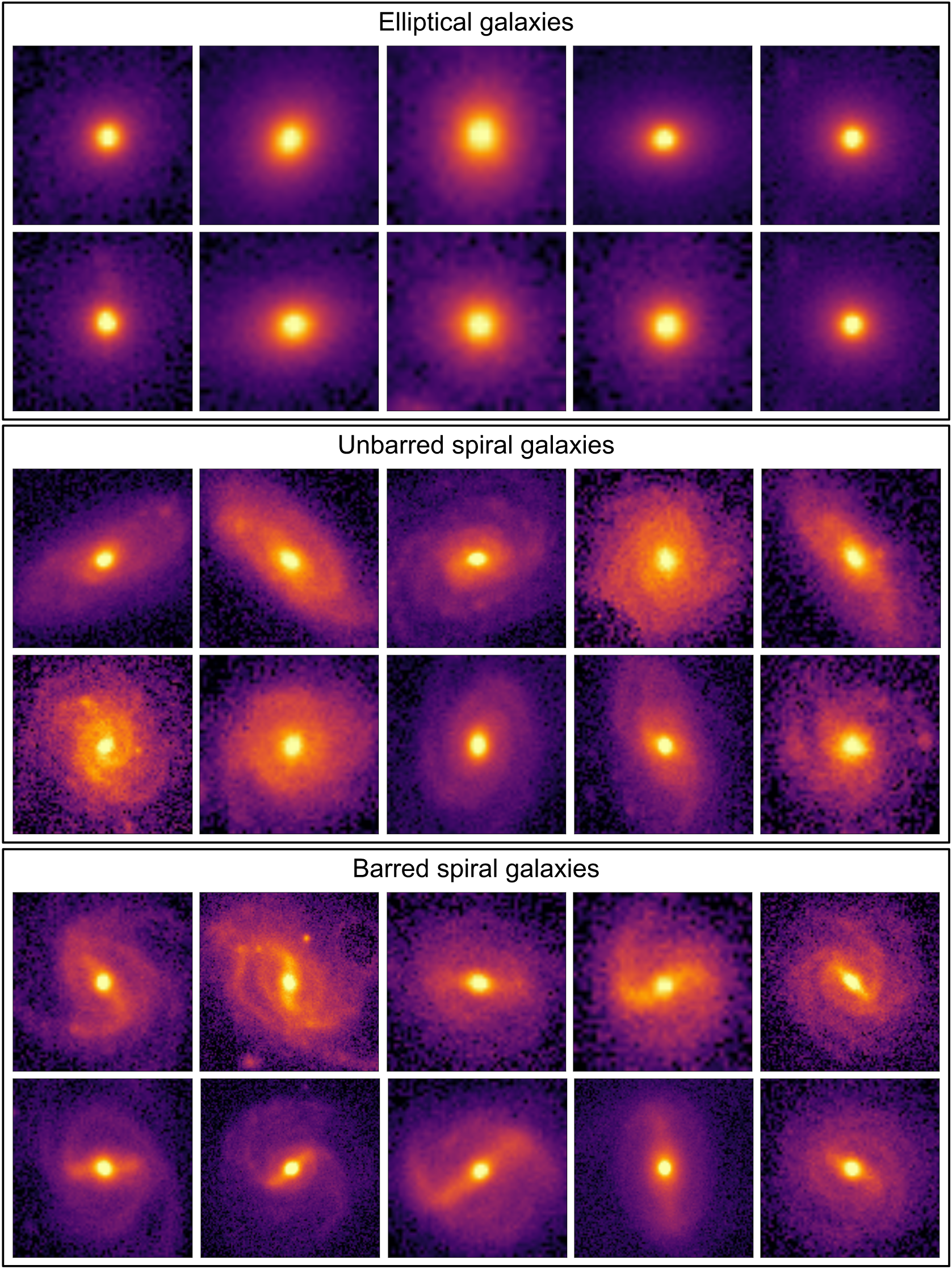
Figure 14: A sample of galaxies classified here in this work using Deep Learning, Galaxy Zoo 2 as supervision (3 classes problem) from $K\geq 10$ dataset. Elliptical galaxies (two top rows), unbarred spirals (two middle rows), and barred spirals (two bottom rows).

References

References

- Abraham et al. (1996) Abraham, R.G., van den Bergh, S., Glazebrook, K., Ellis, R.S., Santiago, B.X., et al., 1996. The morphologies of distant galaxies. ii. classifications from the hubble space telescope medium deep survey. Astrophysical Journal Supplement Series 107, 1. doi:10.1086/192352.
- Baldry et al. (2004) Baldry, I.K., Glazebrook, K., Brinkmann, J., Ivezić, Ž., Lupton, R.H., et al., 2004. Quantifying the Bimodal Color‐Magnitude Distribution of Galaxies. Astrophys. J. 600, 681–694. doi:10.1086/380092.
- Barchi et al. (2016) Barchi, P.H., Sautter, R., da Costa, F.G., Moura, T.C., Stalder, D.H., Rosa, R.R., de Carvalho, R.R., 2016. Improving galaxy morphology with machine learning. Journal of Computacional Interdisciplinary Sciences 7, 114–120. doi:10.6062/jcis.2016.07.03.0114.
- Bertin and Arnouts (1996) Bertin, E., Arnouts, S., 1996. Sextractor: Software for source extraction. Astronomy and Astrophysics, Supplement 117, 393–404. doi:10.1051/aas:1996164.
- Bishop (2006) Bishop, C.M., 2006. Pattern Recognition and Machine Learning (Information Science and Statistics). Springer-Verlag, Berlin, Heidelberg.
- Blanton and Moustakas (2009) Blanton, M.R., Moustakas, J., 2009. Physical properties and environments of nearby galaxies. Annual Review of Astronomy and Astrophysics 47, 159–210. doi:10.1146/annurev-astro-082708-101734.
- Blumer et al. (1987) Blumer, A., Ehrenfeucht, A., Haussler, D., Warmuth, M.K., 1987. Occam’s razor. Information processing letters 24, 377–380. doi:10.1016/0020-0190(87)90114-1.
- Bradley (1997) Bradley, A.P., 1997. The use of the area under the roc curve in the evaluation of machine learning algorithms. Pattern recognition 30, 1145–1159. doi:10.1016/S0031-3203(96)00142-2.
- Collaboration et al. (2016) Collaboration, D.E.S., Abbott, T., Abdalla, F.B., Aleksić, J., Allam, S., Amara, A., et al., 2016. The Dark Energy Survey: more than dark energy - an overview. Monthly Notices of the Royal Astronomical Society (MNRAS) 460, 1270–1299. doi:10.1093/mnras/stw641.
- Conselice (2003) Conselice, C.J., 2003. The relationship between stellar light distributions of galaxies and their formation histories. Astrophysical Journal Supplement Series 147, 1–28. doi:10.1086/375001.
- Conselice et al. (2000) Conselice, C.J., Bershady, M.A., Jangren, A., 2000. The asymmetry of galaxies: Physical morphology for nearby and high-redshift galaxies. Astrophysical Journal 529, 886–910. doi:10.1086/308300.
- Cortes and Vapnik (1995) Cortes, C., Vapnik, V., 1995. Support-vector networks. Machine Learning 20, 273–297. doi:10.1023/A:1022627411411.
- de Carvalho et al. (2017) de Carvalho, R.R., Ribeiro, A.L.B., Stalder, D.H., Rosa, R.R., Costa, A.P., Moura, T.C., 2017. Investigating the Relation between Galaxy Properties and the Gaussianity of the Velocity Distribution of Groups and Clusters. Astronomical Journal 154, 96. doi:10.3847/1538-3881/aa7f2b.
- Dieleman et al. (2015) Dieleman, S., Willett, K.W., Dambre, J., 2015. Rotation-invariant convolutional neural networks for galaxy morphology prediction. Monthly Notices of the Royal Astronomical Society (MNRAS) 450, 1441–1459. doi:10.1093/mnras/stv632.
- Domínguez Sánchez et al. (2018) Domínguez Sánchez, H., Huertas-Company, M., Bernardi, M., Tuccillo, D., Fischer, J.L., 2018. Improving galaxy morphologies for sdss with deep learning. Monthly Notices of the Royal Astronomical Society (MNRAS) 476, 3661–3676. doi:10.1093/mnras/sty338.
- Eisenstein et al. (2011) Eisenstein, D.J., Weinberg, D.H., Agol, E., Aihara, H., Prieto, C.A., et al., 2011. Sdss-iii: Massive spectroscopic surveys of the distant universe, the milky way, and extra-solar planetary systems. Astrophysical Journal 142, 72. doi:10.1088/0004-6256/142/3/72.
- Feigelson and Babu (2006) Feigelson, E.D., Babu, J., 2006. Statistical challenges in astronomy. Springer Science & Business Media.
- Ferrari et al. (2015) Ferrari, F., de Carvalho, R.R., Trevisan, M., 2015. Morfometryka—A New Way of Establishing Morphological Classification of Galaxies. Astrophysical Journal 814, 55. doi:10.1088/0004-637X/814/1/55.
- Freeman et al. (2013) Freeman, P.E., Izbicki, R., Lee, A.B., Newman, J.A., Conselice, C.J., et al., 2013. New image statistics for detecting disturbed galaxy morphologies at high redshift. Monthly Notices of the Royal Astronomical Society 434, 282–295. doi:10.1093/mnras/stt1016.
- Géron (2019) Géron, A., 2019. Hands-On Machine Learning with Scikit-Learn, Keras, and TensorFlow: Concepts, Tools, and Techniques to Build Intelligent Systems. O’Reilly Media, Incorporated.
- Goodfellow et al. (2016) Goodfellow, I., Bengio, Y., Courville, A., 2016. Deep Learning. MIT Press.
- He et al. (2016) He, K., Zhang, X., Ren, S., Sun, J., 2016. Deep residual learning for image recognition, in: The IEEE Conference on Computer Vision and Pattern Recognition (CVPR).
- Hearst et al. (1998) Hearst, M.A., Dumais, S.T., Osuna, E., Platt, J., Scholkopf, B., 1998. Support vector machines. IEEE Intelligent Systems and their Applications 13, 18–28. doi:10.1109/5254.708428.
- Hubble (1926) Hubble, E.P., 1926. Astrophysical Journal 64, 321–369.
- Hubble (1936) Hubble, E.P., 1936. Realm of the Nebulae. New Haven: Yale University Press.
- Huertas-Company et al. (2015) Huertas-Company, M., Gravet, R., Cabrera-Vives, G., Pérez-González, P.G., Kartaltepe, J.S., et al., 2015. A catalog of visual-like morphologies in the 5 candels fields using deep learning. Astrophysical Journal Supplement Series 221, 8. doi:10.1088/0067-0049/221/1/8.
- Huertas-Company et al. (2018) Huertas-Company, M., Primack, J.R., Dekel, A., Koo, D.C., Lapiner, S., et al., 2018. Deep learning identifies high-z galaxies in a central blue nugget phase in a characteristic mass range. Astrophysical Journal 858, 114. doi:10.3847/1538-4357/aabfed.
- Ivezić et al. (2014) Ivezić, Ž., Connolly, A.J., VanderPlas, J.T., Gray, A., 2014. Statistics, Data Mining, and Machine Learning in Astronomy: A Practical Python Guide for the Analysis of Data. Princeton University Press.
- Kaszynski and Piskorowski (2006) Kaszynski, R., Piskorowski, J., 2006. New concept of delay equalized low-pass butterworth filters, in: 2006 IEEE International Symposium on Industrial Electronics, pp. 171–175. doi:10.1109/ISIE.2006.295587.
- Kent (1985) Kent, S.M., 1985. Ccd surface photometry of field galaxies. ii - bulge/disk decompositions. Astrophysical Journal Supplement Series 59, 115–159. doi:10.1086/191066.
- Khalifa et al. (2017) Khalifa, N.E.M., Taha, M.H.N., Hassanien, A.E., Selim, I.M., 2017. Deep Galaxy: Classification of Galaxies based on Deep Convolutional Neural Networks. arXiv e-prints .
- Khan et al. (2018) Khan, A., Huerta, E.A., Wang, S., Gruendl, R., 2018. Unsupervised learning and data clustering for the construction of Galaxy Catalogs in the Dark Energy Survey. arXiv e-prints .
- Kim et al. (2019) Kim, I., Lee, A.B., Lei, J., 2019. Global and Local Two-Sample Tests via Regression. arXiv e-prints arXiv:1812.08927.
- Law et al. (2007) Law, D.R., Steidel, C.C., Erb, D.K., Pettini, M., Reddy, N.A., et al., 2007. The Physical Nature of Rest-UV Galaxy Morphology during the Peak Epoch of Galaxy Formation. Astrophysical Journal 656, 1--26. doi:10.1086/510357, arXiv:astro-ph/0610693.
- Lecun (1989) Lecun, Y., 1989. Generalization and network design strategies. Elsevier.
- Lintott et al. (2011) Lintott, C., Schawinski, K., Bamford, S., Slosar, A., Land, K., et al., 2011. Galaxy zoo 1: data release of morphological classifications for nearly 900 000 galaxies*. Monthly Notices of the Royal Astronomical Society (MNRAS) 410, 166--178. doi:10.1111/j.1365-2966.2010.17432.x.
- Lintott et al. (2008) Lintott, C.J., Land, K., Schawinski, K., Slosar, A., Thomas, D., et al., 2008. Galaxy Zoo: morphologies derived from visual inspection of galaxies from the Sloan Digital Sky Survey*. Monthly Notices of the Royal Astronomical Society (MNRAS) 389, 1179--1189. doi:10.1111/j.1365-2966.2008.13689.x.
- Lotz et al. (2004) Lotz, J.M., Primack, J., Madau, P., 2004. A new nonparametric approach to galaxy morphological classification. Astronomical Journal 128, 163--182. doi:10.1086/421849.
- Martin et al. (2017) Martin, D., Goncalves, T., Darvish, B., Seibert, M., Schiminovich, D., 2017. Quenching or Bursting: Star Formation Acceleration - A New Methodology for Tracing Galaxy Evolution. Astrophysical Journal 842. doi:10.3847/1538-4357/aa71a9.
- Mitchell (1997) Mitchell, T.M., 1997. Machine Learning. 1 ed., McGraw-Hill, Inc., New York, NY, USA.
- Morgan and Mayall (1957) Morgan, W.W., Mayall, N.U., 1957. A spectral classification of galaxies. Publications of the Astronomical Society of the Pacific 69, 291. doi:10.1086/127075.
- Nair and Abraham (2010) Nair, P.B., Abraham, R.G., 2010. A catalog of detailed visual morphological classifications for 14,034 galaxies in the sloan digital sky survey. Astrophysical Journal Supplement Series 186, 427--456. doi:10.1088/0067-0049/186/2/427.
- Nogueira-Cavalcante et al. (2018) Nogueira-Cavalcante, J.P., Gonçalves, T.S., Menéndez-Delmestre, K., Sheth, K., 2018. Star formation quenching in green valley galaxies at 0.5 ≲ z ≲ 1.0 and constraints with galaxy morphologies. Mon. Not. R. Astron. Soc. 473, 1346--1358. doi:10.1093/mnras/stx2399.
- Pedregosa et al. (2011) Pedregosa, F., Varoquaux, G., Gramfort, A., Michel, V., Thirion, B., et al., 2011. Scikit-learn: Machine learning in python. J. Mach. Learn. Res. 12, 2825--2830.
- Pedrini and Schwartz (2007) Pedrini, H., Schwartz, W.R., 2007. Análise de Imagens Digitais: Princípios, Algoritmos e Aplicações. Editora Thomson Learning.
- Petrosian (1976) Petrosian, V., 1976. Surface brightness and evolution of galaxies. Astrophysical Journall 209, L1--L5. doi:10.1086/182253.
- Pozzetti et al. (2010) Pozzetti, L., Bolzonella, M., Zucca, E., Zamorani, G., Lilly, S., et al., 2010. zcosmos - 10k-bright spectroscopic sample - the bimodality in the galaxy stellar mass function: exploring its evolution with redshift. Astronomy and Astrophysics 523, A13. doi:10.1051/0004-6361/200913020.
- Press (2005) Press, S.J., 2005. Applied multivariate analysis: using Bayesian and frequentist methods of inference. Dover Publications.
- Quinlan (1986) Quinlan, J.R., 1986. Induction of decision trees. Machine Learning 1, 81--106.
- Ramos et al. (2000) Ramos, F.M., Rosa, R.R., Neto, C.R., Zanandrea, A., 2000. Generalized complex entropic form for gradient pattern analysis of spatio-temporal dynamics. Physica A: Statistical Mechanics and its Applications 283, 171 -- 174. doi:10.1016/S0378-4371(00)00147-3.
- Roberts and Haynes (1994) Roberts, M.S., Haynes, M.P., 1994. Physical parameters along the hubble sequence. Annual Review of Astronomy and Astrophysics 32, 115--152. doi:10.1146/annurev.aa.32.090194.000555.
- Rosa et al. (2003) Rosa, R.R., Campos, M.R., Ramos, F.M., Vijaykumar, N.L., Fujiwara, S., Sato, T., 2003. Gradient pattern analysis of structural dynamics: application to molecular system relaxation. Brazilian journal of physics 33, 605--610.
- Rosa et al. (2018) Rosa, R.R., de Carvalho, R.R., Sautter, R.A., Barchi, P.H., Stalder, D.H., et al., 2018. Gradient pattern analysis applied to galaxy morphology. Monthly Notices of the Royal Astronomical Society (MNRAS) 477, L101--L105. doi:10.1093/mnrasl/sly054.
- Rosa et al. (1999) Rosa, R.R., Sharma, A.S., Valdivia, J.A., 1999. Characterization Of Asymmetric Fragmentation Patterns In Spatially Extended Systems. International Journal of Modern Physics C (IJMPC) 10, 147--163. doi:10.1142/S0129183199000103.
- Russakovsky et al. (2015) Russakovsky, O., Deng, J., Su, H., Krause, J., Satheesh, S., et al., 2015. Imagenet large scale visual recognition challenge. International journal of computer vision 115, 211--252.
- Sautter (2018) Sautter, R.A., 2018. Gradient Pattern Analysis: New Methodological and Computational Features and Application. Master’s thesis. National Institute for Space Research (INPE). Brazil.
- Sautter and Barchi (2017) Sautter, R.A., Barchi, P.H., 2017. pyghs: Computing geometric histogram separation for binomial proportion patterns. Journal of Computational Interdisciplinary Sciences 8, 121. doi:10.6062/jcis.2017.08.01.0121.
- Schawinski et al. (2014) Schawinski, K., Urry, C.M., Simmons, B.D., Fortson, L., Kaviraj, S., et al., 2014. The Green Valley is a Red Herring: Galaxy Zoo reveals two evolutionary pathways towards quenching of star formation in early- and late-type galaxies. eprint arXiv:1402.4814 .
- Szegedy et al. (2015) Szegedy, C., Liu, W., Jia, Y., Sermanet, P., Reed, S., et al., 2015. Going deeper with convolutions, in: The IEEE Conference on Computer Vision and Pattern Recognition (CVPR).
- Takamiya (1999) Takamiya, M., 1999. Galaxy structural parameters: Star formation rate and evolution with redshift. Astrophysical Journal Supplement Series 122, 109--150. doi:10.1086/313216.
- de Vaucouleurs (1963) de Vaucouleurs, G., 1963. Revised Classification of 1500 Bright Galaxies. Astrophysical Journal Supplement Series 8, 31. doi:10.1086/190084.
- Way et al. (2012) Way, M.J., Scargle, J.D., Ali, K.M., Srivastava, A.N., 2012. Advances in Machine Learning and Data Mining for Astronomy. 1st ed., Chapman & Hall/CRC. doi:10.1201/b11822.
- Willett et al. (2013) Willett, K.W., Lintott, C.J., Bamford, S.P., Masters, K.L., Simmons, B.D., et al., 2013. Galaxy zoo 2: detailed morphological classifications for 304 122 galaxies from the sloan digital sky survey. Monthly Notices of the Royal Astronomical Society (MNRAS) 435, 2835--2860. doi:10.1093/mnras/stt1458.
- Wyder et al. (2007) Wyder, T.K., Martin, D.C., Schiminovich, D., Seibert, M., Budavari, T., et al., 2007. The UV‐Optical Galaxy Color‐Magnitude Diagram. I. Basic Properties. Astrophys. J. Suppl. Ser. 173, 293--314. doi:10.1086/521402.
- Yang and Wu (2006) Yang, Q., Wu, X., 2006. 10 challenging problems in data mining research. International Journal of Information Technology and Decision Making 5, 597--604. doi:10.1142/S0219622006002258.