Statistical Characterization of Hot Jupiter Atmospheres Using Spitzer’s Secondary Eclipses

We report 78 secondary eclipse depths for a sample of 36 transiting hot Jupiters observed at 3.6- and 4.5 $\mu$m using the Spitzer Space Telescope. Our eclipse results for 27 of these planets are new, and include highly irradiated worlds such as KELT-7b, WASP-87b, WASP-76b, and WASP-64b, and important targets for JWST such as WASP-62b. We find that WASP-62b has a slightly eccentric orbit ($e\cos{\omega}=0.00614\pm{0.00064}$), and we confirm the eccentricity of HAT-P-13b and WASP-14b. The remainder are individually consistent with circular orbits, but we find statistical evidence for eccentricity increasing with orbital period in our range from 1 to 5 days. Our day-side brightness temperatures for the planets yield information on albedo and heat redistribution, following Cowan and Agol (2011). Planets having maximum day side temperatures exceeding $\sim 2200$K are consistent with zero albedo and distribution of stellar irradiance uniformly over the day-side hemisphere. Our most intriguing result is that we detect a systematic difference between the emergent spectra of these hot Jupiters as compared to blackbodies. The ratio of observed brightness temperatures, Tb(4.5)/Tb(3.6), increases with equilibrium temperature by $100\pm 24$ parts-per-million per Kelvin, over the entire temperature range in our sample (800K to 2500K). No existing model predicts this trend over such a large range of temperature. We suggest that this may be due to a structural difference in the atmospheric temperature profile between the real planetary atmospheres as compared to models.

1 Introduction

The secondary eclipse of a transiting planet provides an opportunity to measure the planet’s emitted thermal flux in the infrared spectral region (Charbonneau et al., 2005; Deming et al., 2005). When measured over multiple bands, that flux can be used to infer the emergent spectrum of the planet, and numerous investigations have observed and analyzed eclipse photometry for that purpose using the Spitzer Space Telescope (e.g., Charbonneau et al., 2008; Knutson et al., 2009; for a recent review see Alonso, 2018). Ideally, the eclipse could be measured spectroscopically with Spitzer, but Spitzer’s modest aperture has collected sufficient light to allow eclipse spectroscopy for only two of the brightest hot Jupiter systems (Richardson et al., 2007; Grillmair et al., 2008; Todorov et al., 2014). Emergent spectra of several hot Jupiters have been measured near 1.4 $\mu$m wavelength using the Hubble Space Telescope (Kreidberg et al., 2014; Beatty et al., 2017; Cartier et al., 2017; Sheppard et al., 2017; Stevenson et al., 2017; Arcangeli et al., 2018; Kreidberg et al., 2018; Mansfield et al., 2018; Nikolov et al., 2018). The James Webb Space Telescope is projected to obtain emergent spectra for numerous hot Jupiters (Greene et al., 2016; Stevenson et al., 2016; Bean et al., 2018), enabling a major advance in our understanding of their atmospheric physics and chemistry.

In this paper, we set the stage for JWST eclipse spectroscopy of hot Jupiters by reporting a statistical analysis of 27 new hot Jupiters observed in eclipse at both 3.6 $\mu$m and 4.5 $\mu$m using Spitzer. We are currently engaged in a uniform re-analysis of the secondary eclipses of all transiting planets observed by Spitzer. A full report on that re-analysis is not yet possible, so we here apply our uniform analysis to hot Jupiters that have not been previously observed or analyzed in secondary eclipse, supplemented by re-analysis of a few planets that either have special and timely interest, such as HAT-P-13b (Buhler et al., 2016; Hardy et al., 2017), KELT-2Ab (Piskorz et al., 2018), and WASP-18b (Sheppard et al., 2017; Arcangeli et al., 2018), or help us to check our eclipse depths in a statistical sense, such as WASP-14b (Wong et al., 2015). Given recent interest in the hottest of the hot Jupiters (Haynes et al., 2015; Bell et al., 2017, 2019; Evans et al., 2017; Sheppard et al., 2017; Stevenson et al., 2017; Arcangeli et al., 2018; Kreidberg et al., 2018; Mansfield et al., 2018), we have tried to be as complete as possible for the hottest planets. JWST observations of these planets at secondary eclipse will require knowing the orbital phase of their eclipses. Moreover, slightly non-zero eccentricities for the orbits of hot Jupiters, as revealed by the phase of the secondary eclipse, can be diagnostic of their orbital and physical evolution. Hence, we also report and discuss the central phase of the eclipses we analyze. Our work here represents the largest collection of Spitzer’s secondary eclipse depths ever reported in a single paper.

This paper is organized as follows. We describe our observations and photometry procedures in Section 2. Section 3 describes the analysis of the data, beginning with transits of three planets to update their orbital periods (Section 3.1). Sections 3.2 and 3.3 derive eclipse depths and orbital phases by applying pixel-level decorrelation (PLD) to the photometry (Deming et al., 2015). Section 3.4 describes some checks that we have performed to validate our eclipse depths. The eclipse depths of some planets must be corrected for the presence of close companion stars, and those corrections are described in Section 3.5. Section 4 discusses the observed phases of the eclipses, and the implications for orbital dynamics and also for the exoplanetary atmospheres. Section 5 describes how we convert the eclipse depths to brightness temperatures, that are used in the remainder of the analyses. Sec 6 uses those brightness temperatures to study the re-distribution of heat on the planets, and Section 7 compares our measured brightness temperatures to theoretical emergent spectra of the planets. Section 8 summarizes our results and conclusions. An Appendix gives notes on individual planets.

2 Observations and Photometry

The bulk of our observations were made under Spitzer programs 10102, 12085, and 13044 (PI: Drake Deming) in the 2014-2017 time period. We supplement those observations using archival data for planets observed under other programs. Table 1 lists the planets we analyze, and the Astronomical Observation Request (AOR) number of each eclipse. Every planet was analyzed using post-cryogenic 3.6- and 4.5 $\mu$m data from the IRAC instrument. Most planets were observed in subarray mode, yielding 32x32-pixel images in cubes of 64 frames. In addition to observations of secondary eclipses, our Cycle-13 program included observations of transits for many planets. Analysis of the transits is relevant to transmission spectroscopy of these planets, many of which are being observed by HST/WFC3. Although this paper focuses on secondary eclipses, we analyze transits of three planets (Sec. 3.1) in order to improve their orbital ephemerides and thereby derive more accurate secondary eclipse phases.

To perform photometry, we first remove hot pixels in each frame through a 4$\sigma$ rejection applied to each pixel as a function of time. We replace bad pixels with the median value of that pixel over time (see Tamburo et al., 2018 for a discussion of this median-replacement procedure). We estimate the background by first masking the star with a 5x5 pixel box and tabulating the distribution of pixel intensities outside of this box. The center of a Gaussian fit to this distribution is used as the background value. The code produces photometry by first locating the center of the stellar image on the cleaned 32x32 pixel frame with a 2D Gaussian fit. This initial estimate is refined by two methods: a second 2D Gaussian fit or a center-of-light method. The second Gaussian fit is performed on a smaller (4x4 pixel) box surrounding the initial estimate of the centroid. The center of light position is found with an intensity-weighted average of the X and Y positions nearest the initial estimate.

We use the aper procedure in the IDL’s Astronomy User Library to perform the actual aperture photometry, with both fixed-radius and variable-radius apertures methods. Our fixed aperture radii are incremented by 0.1 or 0.2 pixels from 1.6 to 3.5 pixels, producing 11 sets of photometry. The variable radii are computed using the noise-pixel parameter, $\sqrt{\beta}$ from Lewis et al. (2013), added to a constant that ranges from 0.0 to 2.0 pixels, depending on the aperture set of the photometry. The combination of two centering methods, and two aperture radii sets, produces a total of four photometric versions of the secondary eclipse for each visit to a given system. Each version encompasses multiple sets of photometry with different aperture radii. Each photometric point has an associated time extracted from the headers of the FITS files, as BJD(UTC). We carry the UTC-based times through the analysis, and subsequently convert the times of the fitted eclipses to TDB, following Eastman et al. (2010).

3 Extraction of Secondary Eclipse Parameters

3.1 Ephemeris Updates

The time scale for tidal circularization of a hot Jupiter’s orbit is typically much less than the age of the system (Jackson et al., 2008). Observations commonly find hot Jupiter secondary eclipses to be centered very close to phase 0.5 (e.g., Garhart et al., 2018), consistent with a circular orbit. When we find a displacement of the eclipse from phase 0.5, we first check the impact of potential ephemeris error on the observed phase of the eclipse. We found three planets whose ephemerides we were able to update: KELT-7b, WASP-62b, and WASP-74b. We fit Spitzer transits for each planet at both 3.6- and 4.5 $\mu$m using the same procedure as for our eclipse fits (See Section 3.2 below), except that we include quadratic limb darkening based on coefficients in each band from Claret et al. (2013). We freeze the orbital parameters and limb darkening coefficients during the fit, and we vary the ratio of radii (planet-to-star) and the central phase of the transit. Low infrared limb darkening produces a sharp ingress/egress for the Spitzer transits, and facilitates a precise measurement of the transit time. For KELT-7b and WASP-74b, we find that the Spitzer transits are displaced from their predicted phases by amounts that are consistent between the two Spitzer bandpasses, and commensurate with the offsets we encountered for the eclipses. The observed transits and fits are illustrated in Figures 1,  2 and 3. The transit times are given in Table 2, and the transit depths are given in Table 3.

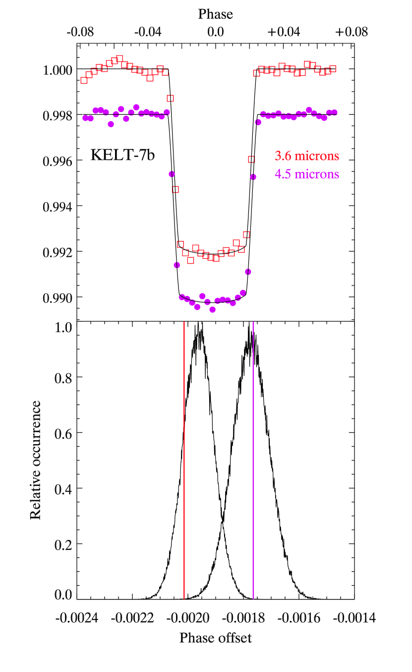
Figure 1: Spitzer transits of KELT-7b. The top panel shows the fit to the data, that are here binned so that 50 points span the range of the data, for clarity and consistency of the illustration. (Our fits were carried out using an alternative binning selected by our code). The lower panel shows the likelihood distributions for the central phase; note that they are significantly offset from the predicted phase of zero, but the two Spitzer wavelengths are in agreement to within the errors. The vertical lines mark the phase of the best fits selected by our MCMC code, see Section 3.2. For this plot, we use the ephemeris given in the discovery paper by Bieryla et al. (2015); see Table 2 for transit times and our updated ephemeris.

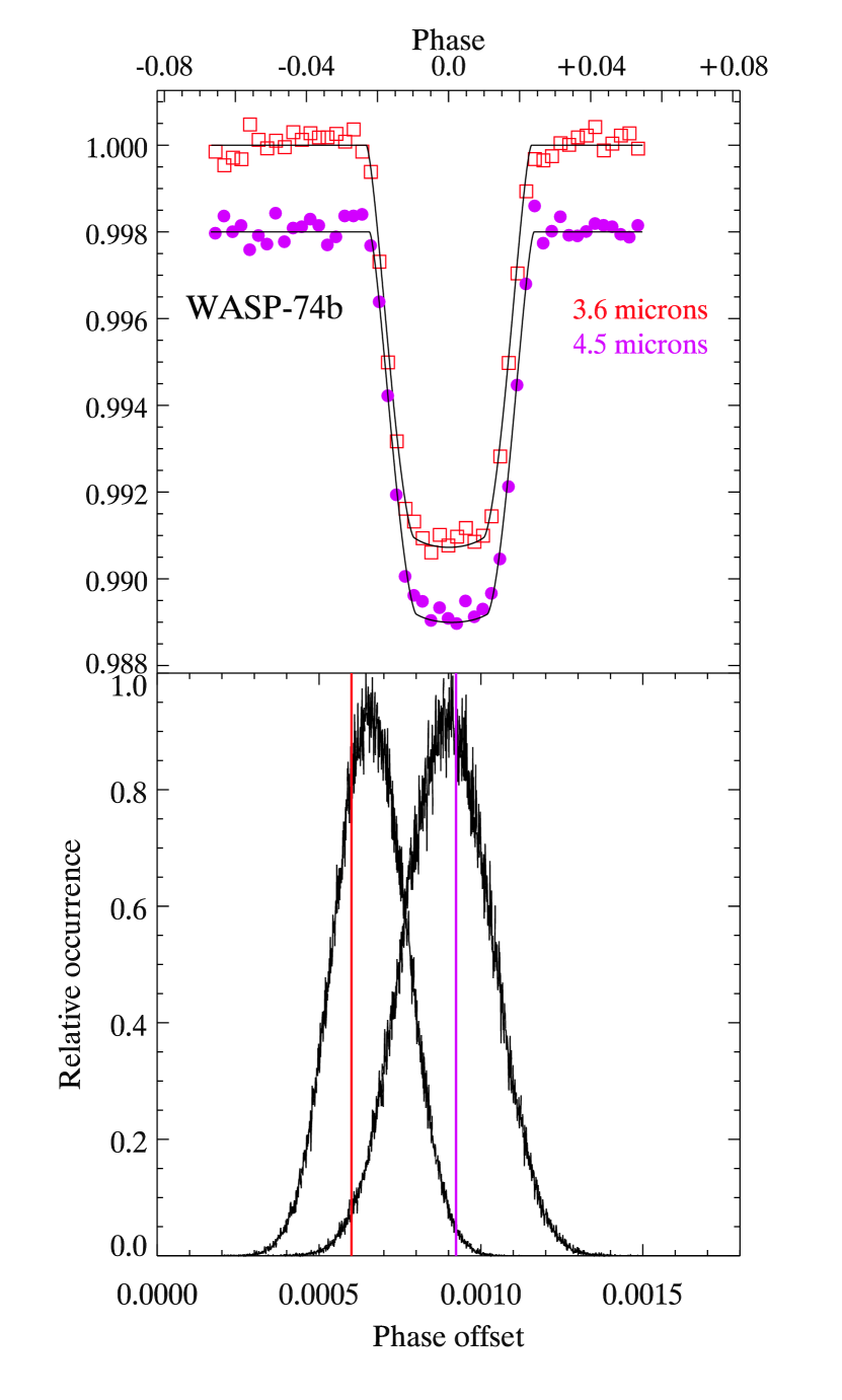
Figure 2: Spitzer transits of WASP-74b. The top panel shows the fit to the data, which are binned so that 50 points span the range of the data for clarity and consistency of the illustration. (Our fits were carried out using an alternative binning selected by our code). The lower panel shows the likelihood distributions for the central phase; note that they are significantly offset from the predicted phase of zero, but the two Spitzer wavelengths are in agreement to within the errors. The vertical lines mark the phase of the best fits selected by our MCMC code, see Section 3.2. For this plot, we use the ephemeris given in the discovery paper by Hellier et al. (2015); see Table 2 for transit times and our updated ephemeris.

We update the orbital periods of KELT-7b and WASP-74b using the Spitzer transit times. For each planet, we use the transit epoch ($T_{0}$) from Bieryla et al. (2015) and Hellier et al. (2015), and we calculate a new period using three points: the epoch listed in the discovery paper, and the transit times from our new Spitzer transits (one at each wavelength). We calculate the period via error-weighted linear least-squares (linfit routine in IDL), and the error on the slope (i.e., the period) follows from the precision of the original $T_{0}$ value and the precision of the Spitzer transit times. The precision of the updated period for KELT-7b is improved by a factor of 8 compared to Bieryla et al. (2015), and for WASP-74b by a factor of 2 compared to Hellier et al. (2015). The Spitzer transit times and updated periods are given in Table 2, and those values are used to calculate the secondary eclipse phases reported in this paper (Section 4).

For WASP-62b, the transits are similarly displaced slightly from the predicted time, as shown on Figure 3. Again, there is excellent agreement between the transits measured independently in both Spitzer bands. We have updated the ephemeris based on the Spitzer transits, and the updated results are included in Table 2. However, even with our updated ephemeris, the eclipses of WASP-62b remain displaced from phase 0.5 due to an eccentric orbit, as discussed in Section 4.

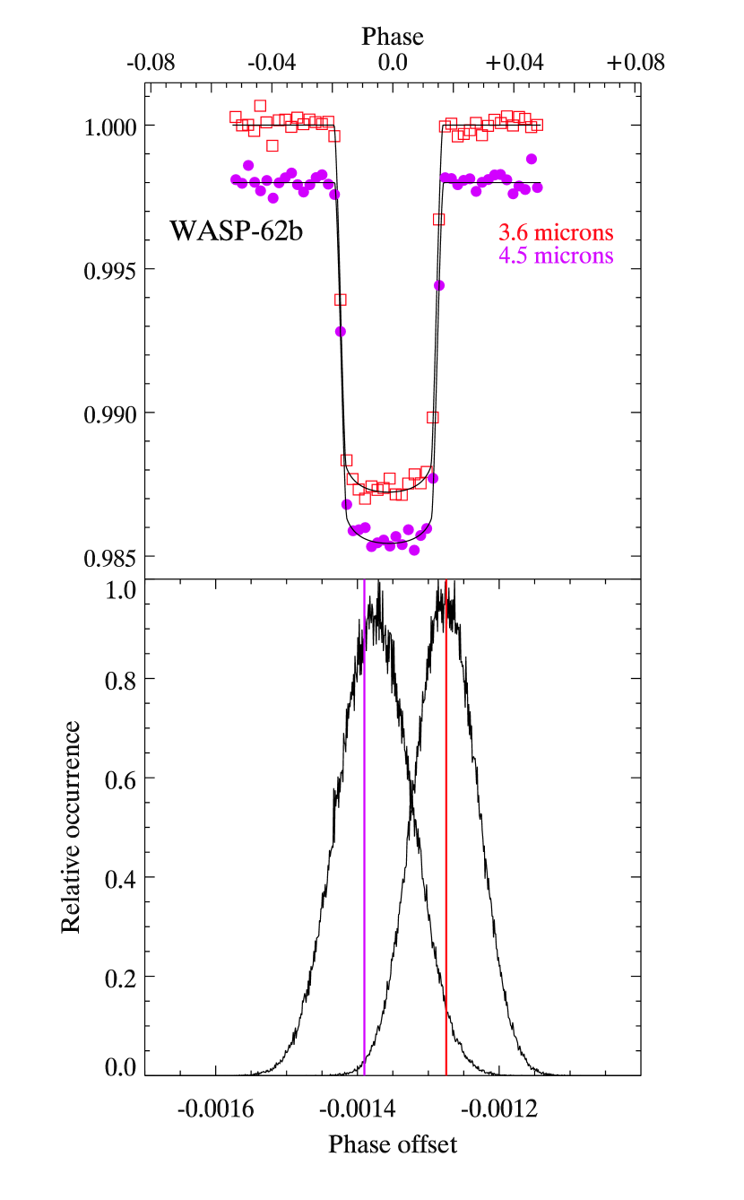
Figure 3: Spitzer transits of WASP-62b. The top panel shows the fit to the data, that are here binned so that 50 points span the range of the data, for clarity and consistency of the illustration. (Our fits were carried out using an alternative binning selected by our code). The lower panel shows the likelihood distributions for the central phase; note that they are significantly offset from the predicted phase of zero, but the two Spitzer wavelengths are in agreement to within the errors. The vertical lines mark the phase of the best fits selected by our MCMC code, see Section 3.2. For this plot, we use the ephemeris given in the discovery paper by Hellier et al. (2012); see Table 2 for transit times and our updated ephemeris.

.

3.2 Analyzing the Photometry

Two major instrumental systematic effects are known to contaminate Spitzer observations and introduce fluctuations in the photometry that can often be an order of magnitude larger than the eclipse being sought. First, there is a characteristic ramping feature that varies with time (Knutson et al., 2012). This ramp-like increase in flux is often most rapid at the beginning of each observation, so by default we omit the first 30 minutes of data from every eclipse to eliminate the potentially steepest portion of the ramp. We model the ramp in the remaining data using either a linear, quadratic, or exponential function of time. We decide between a linear and quadratic ramp model using a Bayesian Information Criterion (BIC) applied to the fitted eclipse. In the (infrequent) cases where the fit is inadequate near the beginning of the time series (judged by structure in the residuals), we either omit 45 or 60 minutes of data instead of the default 30 minutes, or we use an exponential ramp, depending on the characteristics of those specific data.

The second source of noise for Spitzer is the intra-pixel sensitivity variations across the detector. We correct for this effect using Pixel Level Decorrelation (PLD, Deming et al., 2015), and including the temporal ramp as integral to the PLD fitting process. In a Spitzer data challenge, Ingalls et al. (2016) found PLD to have the smallest bias in eclipse measurements as compared to other current decorrelation methods. PLD has been extensively used for Spitzer analyses (Dittmann et al., 2017; Kilpatrick et al., 2017; Buhler et al., 2016; Fischer et al., 2016; Wong et al., 2016; Tamburo et al., 2018), and higher-order PLD is the foundation of the EVEREST code for analysis of K2 photometry (Luger et al., 2016). The PLD formalism was described by Deming et al. (2015), and we do not repeat the equations here. But we summarize that the photometry is modeled as proportional to a linear sum of normalized relative pixel intensities times coefficients determined by the fit, and including the temporal ramp and the eclipse shape. Moreover, our PLD fit uses binned data, because binning averages out small temporal scale fluctuations in the basis pixels, and reduces or eliminates red noise much more efficiently than with unbinned data. Normalizing the pixels is used to remove all astrophysical information from the independent variables in the fitting process. We calculate the shape of the eclipse with an adapted version of the procedure described by Mandel and Agol (2002). As described by Garhart et al. (2018), our version of PLD uses 12 basis pixels, versus the original 9 pixels used by Deming et al. (2015). These 12 pixels are the closest to the median stellar center found in the photometry and generally form a 4x4 pixel box without corners. The eclipse depth is not sensitive to the number of basis pixels per se, but the stars in our sample are sufficiently bright on average that significant flux can be detected in more than the 9 pixels originally used by Deming et al. (2015), and we want to use all significant pixel-level information. Note that Tamburo et al. (2018) used 25 basis pixels for the very bright star 55 Cnc.

3.3 Finding the Eclipse Depth

We here describe the specific procedure that we use when fitting the data to determine the best secondary eclipse depths. Our method is formally Bayesian, but we use uniform priors (see below), so in practice it reduces to a maximum-likelihood calculation. We use the best available orbital parameters for each planet, but we freeze them during the fitting process, varying only the eclipse depth and central phase. That has ample precedent based on many previous secondary eclipse investigations (e.g., O’Rourke et al., 2014; Evans et al., 2015; Mansfield et al., 2018). We use a uniform prior on the eclipse phase that covers the range of the Spitzer observations for each planet.

The duration as well as the phase of a secondary eclipse is affected by non-zero orbital eccentricities (Charbonneau et al., 2005). Anticipating our eclipse phase results (Sec. 4) that constrain eccentricities, and using Eq. (5) of Charbonneau et al. (2005), we calculate that the difference between transit and eclipse duration is not detectable given our precision on the observed eclipses. For planets with known non-zero orbital eccentricities, we nevertheless account for the effect of the eccentricity on the modeled eclipse durations.

An alternative to freezing the orbital parameters would be to use a Gaussian prior for each orbital parameter. However, when those priors are independent of each other, our MCMC (see below) could step to regions of parameter space that would not be acceptable when fitting the transit data, which have much higher S/N than eclipses. For example, the orbital inclination and $a/R_{s}$ are correlated when fitting transits because they both affect the transit duration, and can trade-off against each other. Using uncorrelated Gaussian priors when fitting eclipses allows combinations of inclination and $a/R_{s}$ that are not constrained by the actual transit data. So in those cases there is the danger of using orbital parameters that the transit data would reject. It isn’t practical to fit all of the transit data simultaneously with the large number of Spitzer eclipses that we analyze here. Therefore we continue to fit the eclipses by freezing the best orbital parameters, and varying only the eclipse depth and central phase.

We find the best-fitting eclipse depth and central phase by maximizing the Bayesian posterior probability of each hypothetical depth value, given as:

$$\mathcal{P}_{posterior}\propto\mathcal{L}\times\mathcal{P}_{prior},$$ (1)

where the $\mathcal{P}$ values are the prior and posterior probabilities, and $\mathcal{L}$ is the likelihood, given as:

$$L=\prod_{i=1}^{n}(1/\sqrt{(}2{\pi}{\sigma}^{2}))\exp(-(m_{i}-d_{i})/2\sigma^{2}),$$ (2)

where $d_{i}$ are the data ($n$ photometry points), $m_{i}$ are the modeled photometry points (sum of the eclipse model and the PLD model of the intra-pixel detector sensitivity, see Deming et al., 2015). ${\sigma}$ is the uncertainty assigned to the data points (the same for all points in a given eclipse). Note that Eq.(1) is essentially Bayes’ Theorem, without the denominator (Bayesian evidence, a constant) on the right hand side. Because we freeze the orbital parameters except for eclipse phase, we have:

$$\mathcal{P}_{prior}=1/(\phi_{max}-\phi_{min}),$$ (3)

where $\phi_{max}$ and $\phi_{min}$ are the maximum and minimum orbital phases present in the data. For a given eclipse, $\mathcal{P}_{prior}$ is a constant, and our code maximizes $\mathcal{P}_{posterior}$ by maximizing $\ln{\mathcal{L}}$:

$$\ln{\mathcal{L}}=\sum_{i=1}^{n}{-(m_{i}-d_{i})^{2}/2\sigma^{2}}+constants,$$ (4)

and the right hand side is just the negative of a conventional $\chi^{2}$, plus constants. So for the eclipses we analyze, maximizing $\mathcal{P}_{posterior}$ reduces to minimizing $\chi^{2}$.

Our fitting code uses an initial linear regression to locate the eclipse and estimate the best central phase and pixel coefficients by minimizing the $\chi^{2}$ of a fit to the unbinned data. Then, we freeze the phase of the eclipse, and re-fit for the Spitzer systematics and the eclipse depth using binned data with combinations of aperture radius and bin size, again using linear regression. For each fit to binned data, the code uses the best pixel coefficients and best eclipse depth from the regression to calculate a fit to the unbinned data, and subtracts that to form residuals. The code then calculates the variance (${\sigma}^{2}$) of the residuals as a function of bin size (this is called the Allan deviation relation, Allan, 1966). We adopt the combination of bin size, aperture type and size, and centering method, that minimizes the scatter in the Allan deviation relation (see Garhart et al., 2018). We allow the code to select negative eclipse depths, to eliminate Lucy-Sweeney bias for weak eclipses (Lucy and Sweeny, 1971).

Once the best aperture radius, bin size, and best-fit parameters have been found, they are used to seed a $1x10^{6}$ step Markov Chain Monte Carlo (MCMC) procedure (Ford, 2005) in order to estimate the errors on both the central phase and eclipse depth. We separate the MCMC into three distinct stages: an initial burn-in period of approximately $1x10^{4}$ steps on the unbinned data to find the best step sizes for each parameter. After the burn-in, we re-scale the photometric errors so that the reduced $\chi^{2}$ is $\approx$ 1 for the rest of the analysis.

Approximately $8x10^{5}$ steps are used to fit the binned data and adequately sample the entire parameter space as well as to significantly reduce computation time. Finally, the last $1x10^{4}$ steps also calculate the fit to the unbinned data, and re-compute the Allan deviation relation at each step, so as to possibly find a slightly better solution. The MCMC varies the eclipse phase simultaneously with other parameters in this process (whereas the linear regressions held the phase constant after an initial estimate). Thereby, the MCMC is sometimes able to find a slightly better central phase and eclipse depth value than the linear regressions. We post-process the MCMC chains to calculate the errors on eclipse depth and central phase by fitting Gaussians to the likelihood distributions from the MCMC, and those are virtually always excellent fits.

As mentioned above, there are four sets of photometry for each wavelength. We fit the four versions separately and select the best combination of centering method (Gaussian or center-of-light) and aperture type (fixed or variable radii) by considering the ratio of scatter relative to the photon noise, on both the binned and unbinned time scale. The ratio can vary with bin size, and there is a trade-off between minimizing red noise as opposed to noise on the unbinned time scale. We have not found a rigid formula to implement this trade-off, so subjective judgment is sometimes needed depending on the characteristics of specific eclipses. However, we check to ensure that the eclipse depth is not sensitive (within the errors) to the choice, and we also inspect each fitted eclipse visually to check for potential anomalies in the fit.

In all cases we re-run the code with a different MCMC random seed, to verify convergence to closely similar likelihood distributions of eclipse depth and central phase. Most of our results are based on two MCMC chains per eclipse, each sampling depth and central phase. In some cases we run four MCMC chains in order to further check convergence. We compute the Gelman-Rubin statistic, $R$ (Gelman & Rubin, 1992), for all depth and central phase values based on either two or four independent chains per eclipse. Gelman et al. (2004) suggested that $R$ values less than 1.1 indicate adequate convergence, but exoplanet secondary eclipse work usually achieves values much closer to unity (e.g., Cubillos et al., 2014). Our median $R$ value for the 78 eclipse depths is 1.0023, the average value is 1.0052, and the maximum value is 1.0245. For central phase, the median, average, and maximum $R$ values are 1.0010, 1.0028, and 1.0276.

3.4 Properties and Checks on the Eclipse Solutions

We here describe the properties of our PLD eclipse solutions, and we make a number of checks to ensure the validity of the eclipse depths. Recall that our PLD fitting process operates on binned data, and chooses a ’broad bandwidth’ solution by minimizing the scatter in the Allan deviation relation (see Garhart et al., 2018 and Sec. 3.3 of Deming et al., 2015). We thereby expect that the solutions should be good fits to the data on all time scales, no matter how we bin the data. For clarity of presentation, we bin the data to between 20 and 40 points spanning each data set, and we show all of the eclipses at 3.6 $\mu$m in Figure 22, and all of the 4.5 $\mu$m eclipses in Figure 23. The eclipse of every planet is nominally detected at 4.5 $\mu$m (albeit some with low signal-to-noise), and all except for WASP-75b and WASP-49b are detected at 3.6 $\mu$m (the fitted 3.6 $\mu$m eclipse has a negative depth for WASP-75b and -49b, indicating that the eclipse amplitudes are beneath the noise).

In addition to the eclipse fits shown in Figures 22 and 23, we here explore additional properties of the solutions. The arrangement of pixels relative to the position of the stellar image means that the pixel coefficients in the PLD fitting process can correlate and anti-correlate with each other as the stellar image moves. Given that we expect pixel-to-pixel correlations, a traditional corner plot using the full array of pixel covariances is not particularly useful. However, the eclipse depth should not strongly correlate with any pixel coefficient, since we expect that the pixels will trade-off appropriately in the presence of a stable eclipse depth as the MCMC evolves. Accordingly we illustrate the weakness of correlation between the eclipse depth and pixel coefficients, for two representative eclipses, choosing a strong eclipse (WASP-76b) and a weak eclipse (WASP-131b). Figures 4 and 5 show the likelihood distributions for both eclipse depth and central phase, versus the distributions for the three brightest pixel coefficients. In all cases, no strong correlation is present. Although we illustrate the three brightest pixels, we calculate Pearson correlation coefficients for all 12 pixels versus the depth of each eclipse for one MCMC chain per eclipse, producing $12x78=936$ values. The Pearson values measure the significance of possible correlations, and can be positive or negative, so we work with absolute values. The median Pearson values for the pixel coefficients at 3.6- and 4.5 $\mu$m are 0.0831 and 0.0829, respectively. 85% and 83% of the values are less than 0.2 at 3.6- and 4.5 $\mu$m, respectively. Although the Pearson values are small (perfect correlation would produce unity), they can indicate statistically significant correlations in some cases because each Pearson value is based on $8\times 10^{5}$ samples in an MCMC chain. However, the correlations are weak in the sense that their slope is not sufficient to perturb the eclipse depths significantly, especially since the effects trade-off between pixels.

We track the total effect of the pixel coefficients on the eclipse depth during the evolution of each MCMC chain. We calculate the standard deviation of the effect on eclipse depth, averaged over a time scale of 5000 steps. The median value of those standard deviations, tabulated over all eclipses, is 2.0% of the eclipse depths at 3.6 $\mu$m and 1.5% at 4.5 $\mu$m. We conclude that, although degeneracies between the ramp coefficients and the eclipse depth can contribute significantly to the error on the eclipse depths (see below), the total effect of the pixel coefficients is not significantly degenerate with eclipse depth.

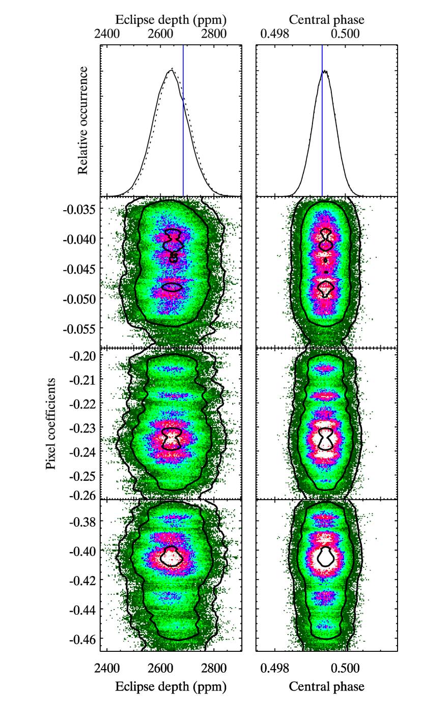
Figure 4: Top panel illustrates the distributions for 3.6 $\mu$m eclipse depth and central phase for WASP-76b. The dashed line (nearly coincident with the solid line) shows nearly identical distributions from duplicate Markov chains with different starting seeds. The vertical lines are the best-fit values chosen by our code, based on minimizing the scatter in the Allan deviation relation. The three lower panels are the distributions for the three brightest pixels in the PLD solutions, versus the distribution of eclipse depth and central phase. The contours are point densities of 0.01, 0.1, and 0.9 of the maximum density. In all cases, the depth and phase are uncorrelated with the pixel coefficients.

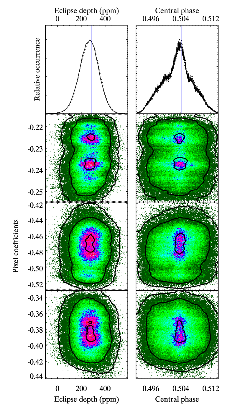
Figure 5: Top panel illustrates the distributions for 4.5 $\mu$m eclipse depth and central phase for WASP-131b. The dashed line (nearly coincident with the solid line) shows nearly identical distributions from duplicate Markov chains with different starting seeds. The vertical lines are the best-fit values chosen by our code, based on minimizing the scatter in the Allan deviation relation. The three lower panel are the distributions for the three brightest pixels in the PLD solutions, versus the distribution of eclipse depth and central phase. The contours are point densities of 0.01, 0.1, and 0.9 of the maximum density. In all cases, the depth and phase are uncorrelated with the pixel coefficients.

Although the derived eclipse depths and phases do not strongly correlate with the PLD pixel coefficients, they do (and should) correlate with the parameters of the temporal ramp, both for the linear and quadratic case. That occurs because the presence of a ramp perturbs the out-of-eclipse reference flux, and it also shifts the centroid of the eclipse. Indeed, the entire point of including the ramp in the solution is to account for such correlations. Figures 6 and 7 show those correlations for WASP-76b and -131b, respectively. The correlations are included in our quoted errors for eclipse depth and central phase (not only for these planets we illustrate but also for all planets we analyze).

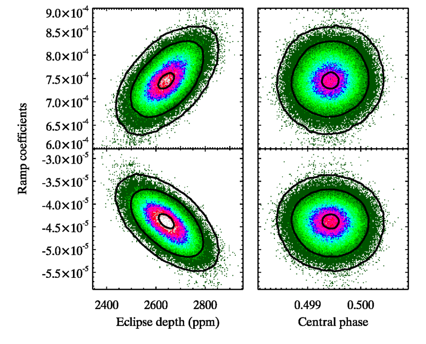
Figure 6: Distributions of the temporal ramp coefficients for WASP-76b at 3.6 $\mu$m, versus the distributions of eclipse depth (left column) and central phase (right column). The top row is the coefficient of $t$ ($t$=time), and the bottom row is the coefficient of $t^{2}$. The contours are point densities of 0.01, 0.1, and 0.9 of the maximum density.

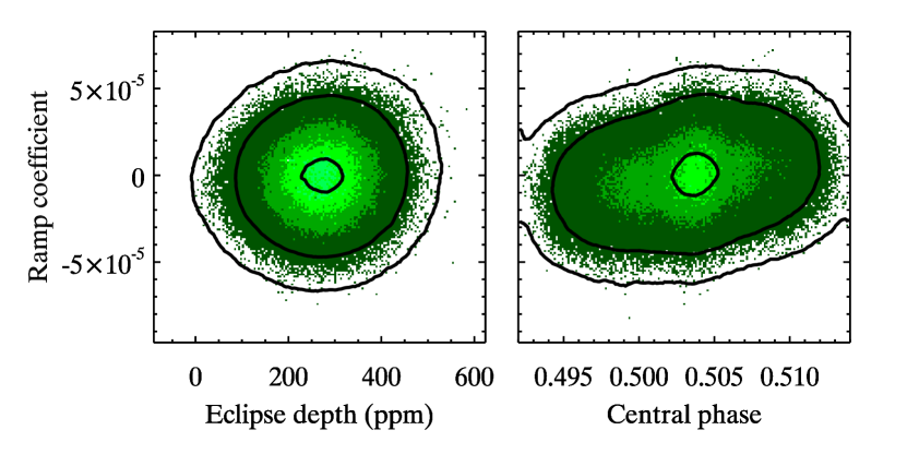
Figure 7: Distributions of the temporal ramp coefficient of $t$ (=time) for WASP-131b, versus the distributions of eclipse depth (left) and central phase (right). (Our WASP-131b eclipse used only a linear, not a quadratic ramp).

An important check on the properties of our solutions for eclipse depth is to examine the amplitude of the residuals (data minus fit) as a function of bin size. Recall that our code fits to binned data, because we find that it helps to reduce red noise. We apply the coefficients from that best fit to the unbinned data, and subtract that fit. We re-bin the residuals with a variety of bin sizes, and calculate the scatter (standard deviation, $\sigma$) of each set of binned residuals for both the binned and unbinned data. Figure 8 shows histograms of this ratio for the unbinned data at both 3.6- and 4.5 $\mu$m. The scatter is always greater than the photon noise; at 3.6 $\mu$m the median ratio is 1.19, and at 4.5 $\mu$m the median is 1.17. The distribution at 4.5 $\mu$m is more strongly concentrated at ratios near unity. At each wavelength, only two eclipses have ratios exceeding 1.5. The bottom panel of Figure 8 shows the ratio of the scatter to the photon noise on the binned time scales that were actually used for each eclipse solution. The median values of that ratio are 1.44 and 1.26 at 3.6- and 4.5 $\mu$m, respectively, but 13 eclipses scatter to ratios above 1.5 at 3.6 $\mu$m, versus 6 at 4.5 $\mu$m. We conclude that the eclipse solutions are giving good performance over a wide range of time scales. Note also the ratio of scatter to the photon noise does not correlate with the bin time on the bottom panel of Figure 8, indicating that the scatter is decreasing versus bin size with approximately the same functional behavior for all eclipses.

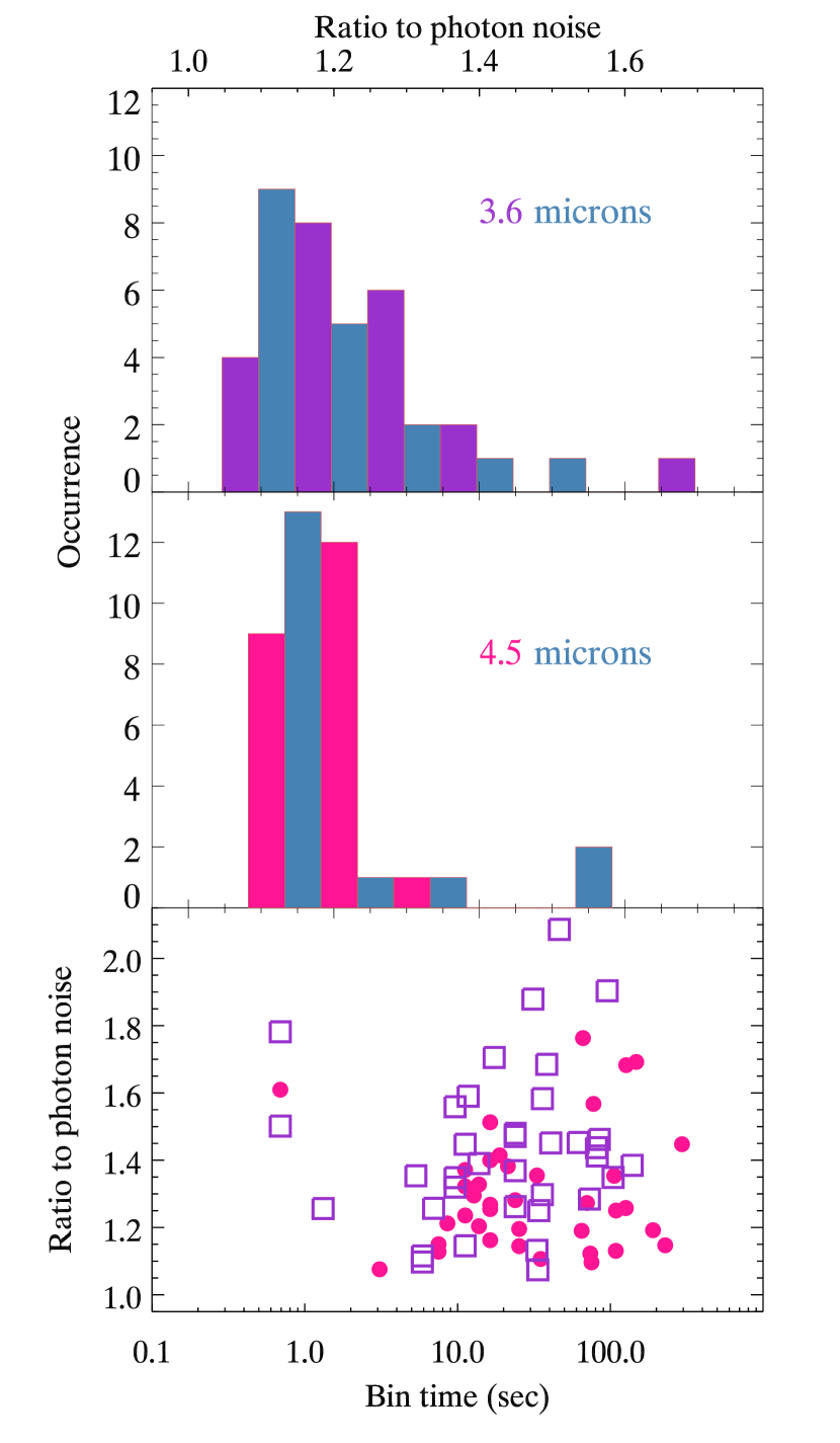
Figure 8: The upper two panels (read upper axis scale) show histograms of the ratio of the unbinned scatter in our residuals to the photon noise for all eclipse depth solutions (each planet contributes one point to each histogram). Alternate colors for adjacent histogram bins are used solely for visual clarity. The bottom panel (read lower axis scale) shows the ratio of the scatter to the photon noise on the binned time scale used for each eclipse solution, versus the bin time for that solutions. Point colors identify the wavelength, as per the two upper panels.

Another way to view the noise performance of the eclipse solutions is from the slope of the Allan deviation relation, i.e. the standard deviation of the binned residuals as a function of bin time. Histograms of the Allan deviation slope are shown for both wavelengths in Figure 9. For photon-limited performance, the standard deviation ($\sigma$) should decrease as the square root of the bin size with a slope of -0.5 in log space. If, for example, we were to over-fit the data, then we might find the slope to be consistently less than -0.5, which is not physically possible for a valid fitting process (because we cannot overcome the photon noise). The distributions of Allan deviation slope over all of our eclipse depth solutions are therefore useful diagnostics of our fitting procedure. Figure 9 shows histograms of the slopes for the 3.6- and 4.5 $\mu$m eclipses. The median value for the 3.6 $\mu$m slopes is -0.45 and for 4.5 $\mu$m it is -0.48. Both distributions decrease strongly at -0.5, albeit with some values approaching -0.54. Our 3.6 $\mu$m solutions have 4 slope values less than -0.5, but all of them greater than -0.53. At 4.5 $\mu$m, 6 slopes are less than -0.5, with the smallest value being -0.537. The slope has its own intrinsic uncertainty, averaging to 0.013 at both wavelengths. No individual slope is below -0.5 by 3 or more times its individual standard deviation. We conclude that the values falling below -0.5 are due to random fluctuations, and that our eclipse depth solutions approach closely to the photon noise limit, but we are not over-fitting.

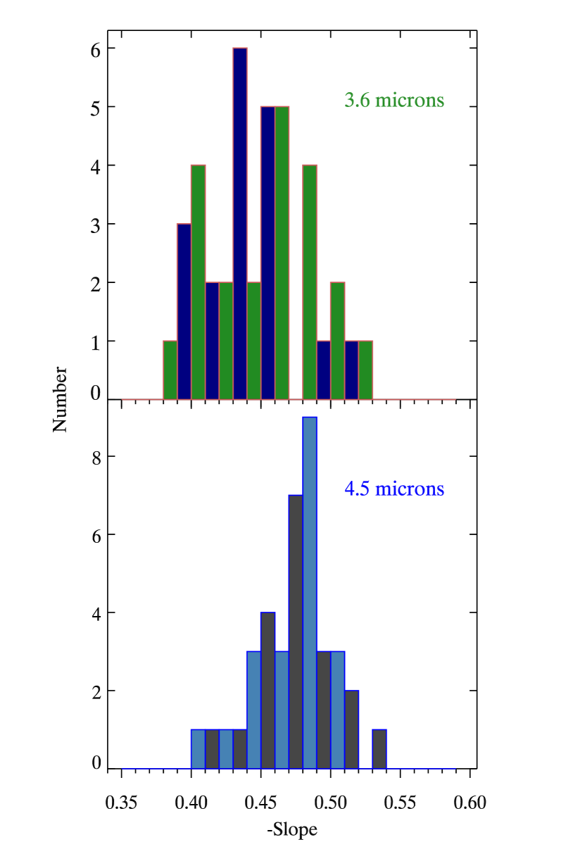
Figure 9: Histograms of the Allan deviation slope for our collection of eclipse depth solutions. Alternate colors for adjacent histogram bins are used solely for visual clarity. The top panel shows the distribution at 3.6 $\mu$m, and the bottom panel at 4.5 $\mu$m.

As described above, we examine four different versions of the photometry at each wavelength, independently choosing the best overall fit from among them for each planet and each wavelength. Thus we might adopt Gaussian centroiding with variable-radius photometry apertures at 3.6 $\mu$m for a given planet, and center-of-light centroiding with constant-radius apertures for the same planet at 4.5 $\mu$m. Our rationale is that each data set is different, and has unique characteristics that require flexibility in the fitting process. Nevertheless, a strength of our work is that we analyze eclipses for 27 new planets using a uniform methodology, to facilitate accurate statistical conclusions. In light of that goal, it may seem odd that we utilize one of four different sets of photometry for each planet at each wavelength. Does this variation destroy the uniformity of our analysis, and introduce additional noise or systematic effects? To investigate that possibility, we compare our adopted eclipse depths with the eclipse depths that are derived always using Gaussian centroiding and constant-radius apertures (hereafter, Gaussian-constant = GC). One way to evaluate uniformity is to compare each set of eclipse depths with some physical variable that is independent of our data analysis, but should correlate with eclipse depth. Whatever the shape of that functional relation, the best set of eclipse depths should exhibit less scatter. We use the equilibrium temperature of each planet as the independent variable, calculated assuming zero albedo, a circular orbit, and uniform distribution of heat. We remove the effect of different stellar and planetary radii, and the stellar temperature, by dividing each measured eclipse depth (not including the dilution correction described in Sec. 3.5) by the ratio of planetary to stellar disk areas. We also multiply by the stellar intensity, using a blackbody at the stellar effective temperature (a good approximation at these wavelengths). We multiply the result by 100 to put the numbers on a convenient scale. These scaled eclipse depths are shown at 3.6- and 4.5 $\mu$m in Figure 10. As expected, both sets of eclipse depths correlate with equilibrium temperature, albeit not a purely linear relation (the exact shape of the relation is unimportant for our immediate purpose).

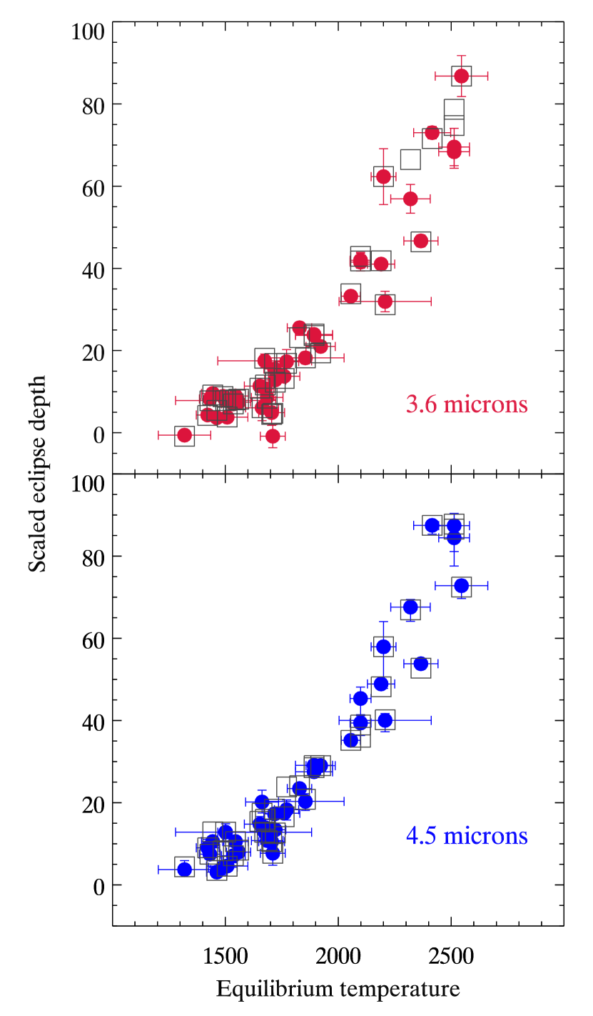
Figure 10: Scaled eclipse depths (see text) versus the equilibrium temperature of each planet. The purpose of this comparison is to check the consistency and relative scatter between our adopted eclipse depths (solid points with error bars), and the eclipse depths derived always using Gaussian centroiding and constant-radius photometric apertures (GC depths). The GC depths are plotted as open squares without error bars. Both sets of eclipse depths are in excellent agreement, and exhibit similar levels of scatter.

Interestingly, the GC eclipse depths yield virtually the same correlation on Figure 10, with the same scatter, as do our adopted eclipse depths. This shows that we are not introducing a source of significant non-uniformity when choosing from among four different sets of photometry, but neither are we significantly improving the results. To investigate further, we calculated the linear regression relation between the GC depths and our adopted depths. A maximum likelihood regression (see below) with the adopted depths as Y and GC depths as X yields a slope of $1.0079{\pm}0.0135$, and an intercept of $-22\pm 28$ ppm, with a tight relation (not illustrated). The scatter from that relation is virtually the same (close to 220 ppm) in each coordinate, suggesting that the two sets of eclipse depths have approximately the same uniformity. We conclude that our procedure of choosing among four alternate sets of photometry does not degrade the uniformity of our results, but neither does it improve it significantly. Given that different data sets can have potentially very different characteristics, we consider it prudent to use our adopted depths in our analyses reported below, but we also check the results using the GC depths. Finally, we also have a third set of eclipse depths, obtained as the centroid of the distribution for eclipse depth, rather than the specific value selected using our Allan deviation slope criterion. Those centroid-of-the-distribution (CD) depths are very close to our adopted values, as can be seen by comparing the vertical lines to the distributions on the top left panels of Figure 4 and Figure 5.

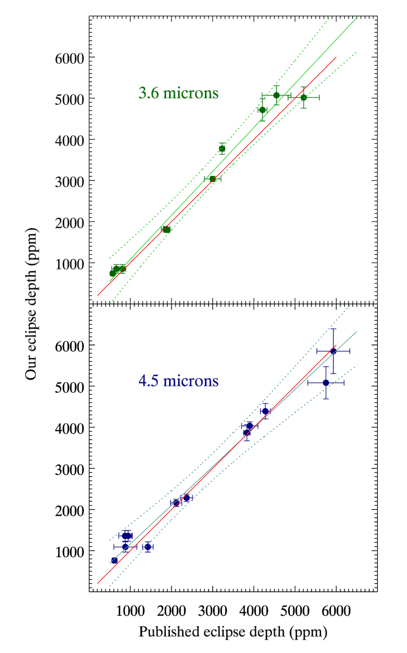
Figure 11: Comparison between our derived eclipse depths and previously published results, for seven planets at 3.6 $\mu$m, and adding WASP-62b at 4.5 $\mu$m. The red lines represent slopes of unity, i.e. perfect agreement. The solid lines in the same color as the points are the results of maximum likelihood regressions, considering errors in both coordinates. The regression lines are of the form: $y-\overline{y}=a(x-\overline{x})+b$, where $\overline{x}$ is the average value. The regression values of $a$ and $b$ are $1.068\pm 0.081$ and $22\pm 120$ at 3.6 $\mu$m. The 4.5 $\mu$m regression values are $0.945\pm 0.066$ and $25\pm 101$. The dotted lines are the $\pm 3{\sigma}$ limits on departures from the regression lines.

Finally, we examine how our eclipse depths correlate with values published in the peer-reviewed literature. We make this comparison for seven planets at 3.6 $\mu$m and eight planets at 4.5 $\mu$m. These planets and their previous eclipses are: HAT-P-13b observed by both Hardy et al. (2017) and Buhler et al. (2016), KELT-2b (Piskorz et al., 2018), WASP-12b (Stevenson et al., 2014), WASP-14b (Wong et al., 2015), WASP-19b (Wong et al., 2016), and WASP-43b (Stevenson et al., 2017). At 4.5 $\mu$m, we added WASP-62b (Kilpatrick et al., 2017). Details of our comparisons for some of these cases are discussed under the notes for individual planets in the Appendix. Although we have analyzed WASP-103b (Kreidberg et al., 2018), we omit it from our comparison, for the reason discussed in the notes for that planet.

Figure 11 shows the comparisons between our eclipse depths and published values at both wavelengths. Taking the published values as the independent variable ($x$), and our values as the dependent variable ($y$), we calculate the slope and zero-point of a linear relation, using the maximum likelihood regression method described by Kelly (2007), and accounting for errors in both $x$ and $y$. The solutions also yield the standard deviation of slope and intercept. A main result of this paper is a systematic trend in exoplanetary brightness temperatures as a function of equilibrium temperature (Section 7.3). Since planets with the highest equilibrium temperatures tend to have the greatest eclipse depths, we want to verify that our main result will not be contaminated by a systematic error that trends with eclipse depth. Comparing to previously published results, we expect to find slopes near unity, and small intercepts. The maximum likelihood regressions yield slopes and intercepts that are in $1-\sigma$ agreement with unity and zero, respectively - see the caption of Figure 11. We conclude that our eclipse depths do not deviate systematically from previous work.

3.5 Dilution Corrections

Our photometry is normalized to unity during eclipse. When a stellar companion is present, that normalization can include contaminating light from the companion, thus requiring a dilution correction applied to the measured eclipse depths. We identify systems needing dilution correction by inspecting the Spitzer images themselves, and by consulting results from high resolution imaging (Ngo et al., 2015, 2016; Wollert et al., 2015; Wollert & Brandner, 2015; Evans et al., 2018).

For systems with identified companions, we multiply our fitted eclipse depths times a dilution correction factor $f_{d}$ given as:

$$f_{d}=1+f_{s}r_{s},$$ (5)

where $f_{s}$ is the fraction of the light from the companion star that is scattered or diffracted into the photometric aperture centered on the target star (or completely in the aperture in some cases), and $r_{s}$ is the ratio of the total brightness of the companion star to the total brightness of the target star in a given Spitzer band. Multiplying our fitted eclipse depth times $f_{d}$ yields the true astrophysical eclipse depth. Twelve of the systems we analyze have stellar companions that are sufficiently bright and close that $f_{d}$ significantly exceeds unity. Those twelve systems are listed in Table 4, with our calculated $f_{d}$ factors.

The twelve systems listed in Table 4 can be divided into two groups. First, there are WASP-12, -49, -76, -103, HAT-P-33, and KELT-2, whose stellar companions are entirely contained in the photometric aperture used for our Spitzer photometry ($f_{s}=1$). The remainder of the Table 4 systems have companions that contribute only a fraction of their light to our photometric aperture ($f_{s}<1$).

For this second group, we determined $f_{s}$ by placing an aperture at a position adjacent to the target star, choosing the location to be symmetrically opposite the contaminating star. For example, if the contaminating star is 4 pixels below the target star, we place our aperture 4 pixels above the target star. Our assumption is that the point-spread-function for the target star and the companion are the same, because they are both very close to the center of Spitzer’s field of view. In that case, the fraction of target light scattered or diffracted into our symmetric aperture will be the same as the fraction of companion light scattered or diffracted into the target aperture. Also, the symmetric aperture is sufficiently distant from the companion star to be unaffected by light from the companion. We choose the symmetric aperture to have the same size as the target aperture. Figure 12 illustrates this method. For cases where we use a variable-radius aperture on the target star, we use a symmetric aperture having a constant radius closest in size to the median value of the variable aperture used for the target.

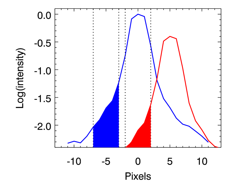
Figure 12: Illustration of our method to define the effect of scattered or diffracted light from stellar companions lying outside of the photometric aperture (illustrated here in 1-D). The bounds of the photometric aperture are shown as dashed lines at $\pm 2$-pixels. The red curve is the companion star, several times fainter than the target star (blue curve). The red and blue curves have the same shapes (PSFs), given their close proximity in the focal plane. The companion star light scattered into the photometric aperture is shaded in red. We place a second aperture symmetrically located opposite to the companion star (dashed lines centered on $-5$-pixels), and we measure the light from the target star scattered into this symmetric aperture (shaded blue region). Since the companion star contributes negligibly to the symmetric aperture, the ratio of the shaded blue region to the peak (or integral) of the blue curve equals the corresponding ratio for the red region and curve. The peak intensities of each curve (and integrals) are readily measured for each image, but we use average values for the entire time series. We thereby solve for the amount of companion light in the shaded red region of each exposure without requiring complex manipulations of the data, and without needing to assume an analytic expression for the wings of the PSFs.

From the time series photometry, we determine the median value of the flux in the symmetric aperture, after subtracting a background value, and we divide that by the median background-subtracted flux measured for the target star, and the ratio of those fluxes is $f_{s}$. In the cases where the companion star is spatially separated from the target in the Spitzer images, we calculate $r_{s}$ by fitting 2-D Gaussian functions to both stars, and calculate $r_{s}$ as the ratio of the areas under those Gaussians.

The procedure described above does not require independent measurements of the spectral type or magnitude difference between the target and companion star. Instead, we measure $r_{s}$ directly from the Spitzer data. However, for WASP-12, -49, -76, -103, HAT-P-33, and KELT-2, the companion stars are too blended with the target to make that direct measurement, and for HAT-P-30 the blend is also problematic. In those cases, we estimate $r_{s}$ in the Spitzer bands based on the difference in K-magnitudes, and the spectral types (effective temperatures) given by various sources (see the Appendix). From those magnitudes and effective temperatures, we calculate the flux ratio in the Spitzer bandpasses by interpolating among values output by the STAR-PET online calculator.

In addition to the correction factors listed in Table 4, WASP-49 and WASP-121 have other stars at 9 and 7 arcsec distant, respectively, (Lendl et al., 2012; Delrez et al., 2016), Those companions are too faint and too distant in sky separation to significantly contaminate our Spitzer observations, and no dilution correction is required.

Our dilution correction factors listed in Table-4 have not been applied to the ’as-measured’ eclipse depths listed in Table 1. However, they have been applied before we use the Table 1 values in our subsequent analyses.

4 Results for Orbital Phase

Previous secondary eclipse observations have shown that the majority of transiting hot Jupiters have orbital eccentricities close to zero due to tidal circularization (e.g., Baskin et al., 2013; Todorov et al., 2013; Beatty et al., 2014; Deming et al., 2015; Garhart et al., 2018).

Our results are consistent with that trend. The times and orbital phases of our observed eclipses are listed in Table 5. The top panel of Figure 13 shows our measured central phase for all of the eclipses we measure, corrected for light travel time across the orbit (a small effect, about $0.0002$ in phase), and plotted versus the orbital period of the planet. For all planets, we add the precision of their orbital ephemerides in quadrature with the observed phase error to produce the error bars for phase on the figure. Two planets on Figure 13 are already known to have eccentric orbits: WASP-14b (Blecic et al., 2013; Wong et al., 2015), and HAT-P-13 (Buhler et al., 2016; Hardy et al., 2017). WASP-14b is labeled on the top panel of the figure.

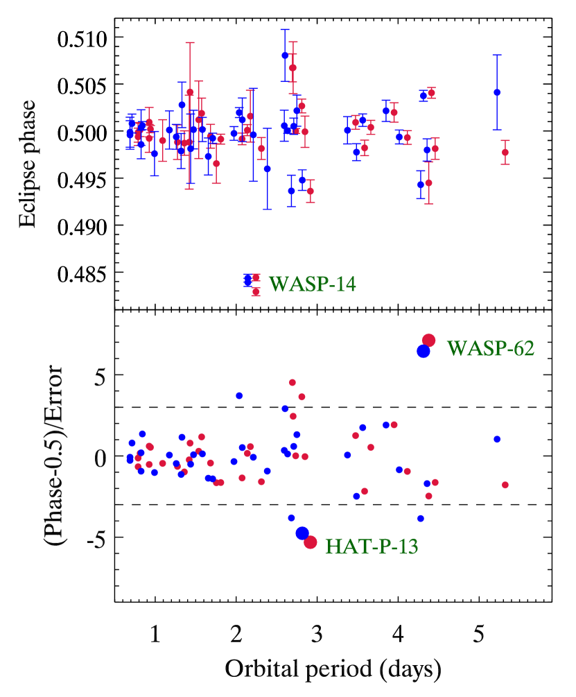
Figure 13: The top panel plots the measured orbital phase of our secondary eclipses, corrected for light travel time across the orbit, versus the orbital period of each planet. Error bars include our measurement error and also imprecision in the orbital ephemerides. Red points are 3.6 $\mu$m and blue are 4.5 $\mu$m. WASP-14b (labeled) is known to have an eccentric orbit, so the central phase deviates from 0.5. The lower panel plots the phase minus 0.5, divided by the error on the phase. The scale of the ordinate is expanded, so WASP-14 is off-scale, and HAT-P-13 and WASP-62 are labeled (larger points). Note the prominent deviation of WASP-62b due to a slightly eccentric orbit. Horizontal dashed lines mark $\pm 3\sigma$.

The bottom panel of Figure 13 plots the deviation from phase 0.5 divided by the precision of the measurement (including ephemeris error), again versus the orbital period. The scale of the ordinate is expanded, so that WASP-14b is now beyond the limits of the plot. HAT-P-13b is labeled on this bottom panel, and also WASP-62b is labeled and has a clearly detected orbital eccentricity. Spitzer eclipse phases for WASP-62b agree very well between the two independent measurements, and the high statistical significance of the deviations ($>6\sigma$) makes the planet very obvious on the bottom panel of Figure 13. The two measured phase values, corrected for light travel time are $0.50406\pm{0.00057}$ and $0.50375\pm{0.00058}$ at 3.6- and 4.5 $\mu$m respectively. The quoted errors again include imprecision in our improved ephemeris. Weighting the phase in each band by the inverse of its variance yields an average orbital phase of $0.50391\pm{0.00041}$; the corresponding value of $e\cos{\omega}$ is $0.00614\pm{0.00064}$. The orbital eccentricity of this planet is especially important because it is in the continuous viewing zone for JWST. The eclipse occurs about 23 minutes later than phase 0.5, and that could potentially cause a significant degradation in JWST spectroscopy if the eclipse were incorrectly assumed to occur exactly at phase 0.5.

We have investigated whether the secondary eclipse phase deviates systematically from phase 0.5 at longer orbital periods, due to incomplete tidal circularization at greater orbital distances. Figure 14 shows the absolute deviation of the eclipse phase from 0.5, versus orbital period. A least-squares fit accounting for the errors in phase yields a slope of $0.00043\pm{0.000072}$, if we ignore WASP-14b that would otherwise dominate the fit. On that basis, the eclipse phase (on average) deviates from 0.5 by 0.00043 for each 1-day increase in orbital period. If we also ignore WASP-62b and HAT-P-13b, the fitted slope becomes $0.00024\pm{0.000078}$. However, those three planets are unambiguous examples of eccentric orbits, so ignoring them is ignoring the effect that we seek. The fitted slope being $3\sigma$ above zero even when the obvious eccentric planets are ignored, is evidence for a lack of tidal circularization, increasing with orbital period in the range of our sample (0.8 to 5.5 days). However, the significance of the slopes depends on whether the distribution of central phases is Gaussian. Ignoring the clearly eccentric planets, we applied an Anderson-Darling test to the distribution of central phases. This indicates a lack of normality (p-value of $10^{-4}$). That occurs because there are outliers, even after eliminating the clearly eccentric planets. Small amounts of orbital eccentricity in our sample could cause those outliers, and thereby contribute to failing the Anderson-Darling test. Moreover, the central portion of the phase distribution (within $\pm{2}\sigma$, comprising the majority of the phases) does pass the Anderson-Darling test, as described below. Hence we tentatively conclude that there is valid evidence for eccentricity increasing with orbital period. However, eclipse phases are also sensitive to imprecision in orbital ephemerides, so this issue should be re-visited when more precise transit times and orbital periods become available (i.e., adding TESS data).

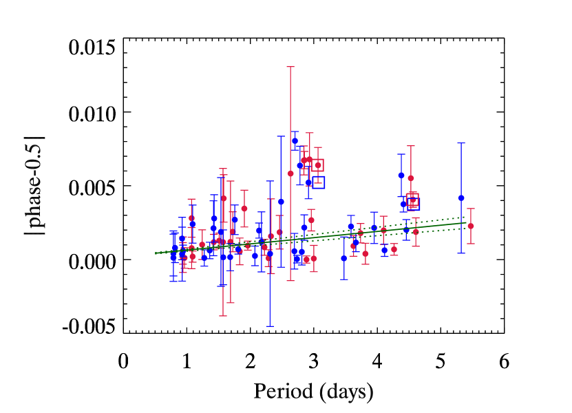
Figure 14: Absolute deviation of the secondary eclipse phase from 0.5, versus orbital period in days. The green line is a least-squares fit, ignoring WASP-14b (that is off scale). Dotted lines indicate the $\pm{1}\sigma$ error on the slope. Planets with well established eccentric orbits (HAT-13b and WASP-62b) are plotted with open squares to distinguish them, and without error bars to minimize confusion.

Figure 15 shows distributions of the phase offset from 0.5 for most planets, normalized by the error of each measurement, i.e., a histogram of the values plotted in the lower panel of Figure 13. When constructing the histograms, we omitted WASP-14, WASP-62 and HAT-P-13, so the histograms represent only planets whose potential orbital eccentricity is not detected. The green curves are the result of fitting Gaussian functions to the distributions defined by these histograms. Fitting Gaussians to these binned distributions is a good way of measuring the dispersion in the central portion of the distribution, with minimal sensitivity to outliers. As noted above, the total phase distributions are not Gaussian, because they fail an Anderson-Darling test. That failure occurs because there are more outliers than expected for a Gaussian distribution. Repeating the Anderson-Darling test for phases within $\pm 2$ standard deviations of 0.5 shows good normality (p-values of 0.60 and 0.75 at 3.6- and 4.5 $\mu$m, respectively). If all planets represented in the central portions of the distributions have tidally circularized orbits with zero eccentricity, and if our errors are correctly estimated, then the fitted Gaussians should be centered at zero, with standard deviations of unity. The fitted Gaussian functions come close to that expectation, but differ slightly. The standard deviations of the Gaussians at 3.6- and 4.5 $\mu$m are 1.13 and 1.19, respectively. Given that those values exceed unity in both Spitzer bands, and given the evidence discussed above for eccentricity increasing with orbital period, we conclude that there may be a small amount of undetected orbital eccentricity in our sample of planets. We emphasize that this conclusion is tentative and should be re-visited when more eclipses are analyzed, especially using improved ephemerides from TESS.

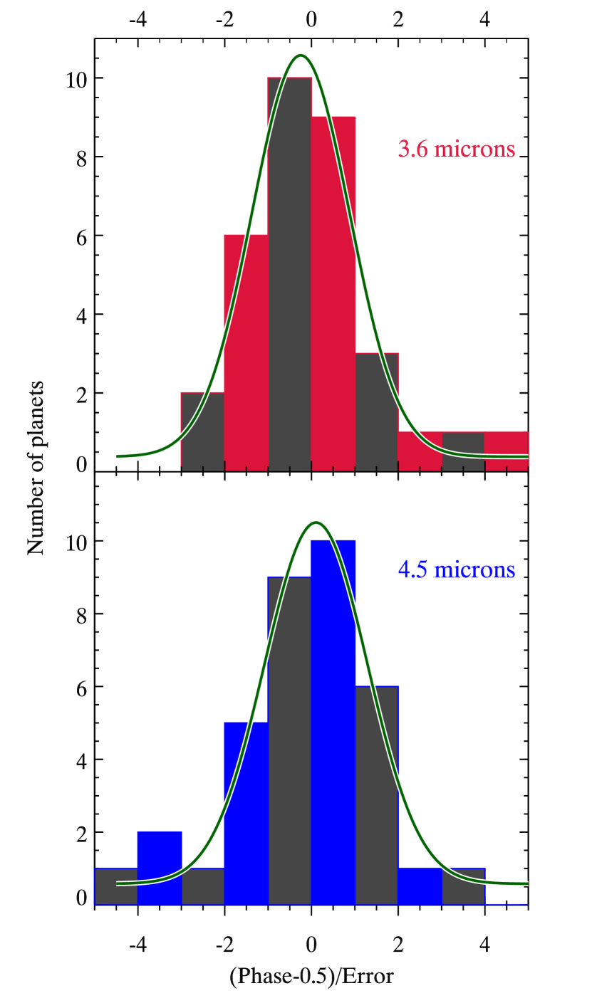
Figure 15: Histograms of the deviation of our measured phase from 0.5, normalized by the error bar (i.e, histograms of the points on the lower panel of Figure 13. Alternate colors for adjacent histogram bins are used solely for visual clarity. We omit eccentric planets (WASP-14, WASP-62 and HAT-P-13). The green curves are best-fit Gaussians (see text).

We are also interested in whether the average phase deviates from 0.5 systematically in one direction, such as the ”uniform time offset” effect described by Williams et al. (2006). Although the binned histograms in Figure 15 are good visual representations, and a good way of evaluating the scatter in the data compared to our estimated errors, they are not optimum for measuring potential systematic displacement. The binning process slightly distorts the distributions (Kipping, 2010), and they effectively weight each measured phase by the inverse of its standard deviation, whereas correct weighting is proportional to the inverse of the variance (variance = standard deviation squared). So we also use the original phase data (top panel of Figure 13), and we compute the average phase, correcting for light travel time and weighting each measurement by the inverse of its variance. We again omit WASP-14, WASP-62, and HAT-P-13. We find average eclipse phases of $0.499969\pm{0.000157}$ and $0.500355\pm{0.000176}$ at 3.6- and 4.5 $\mu$m, respectively. If we combine the bands, we derive a grand average phase of $0.500140\pm{0.000118}$. Note that even with slightly non-zero eccentricities, the average phase should indeed be very close to 0.5, because $\omega$ is effectively random.

Only with the uniform time offset effect described by Williams et al. (2006) would we expect to detect an average difference from phase 0.5. However, we find no statistically significant difference. Considering the average orbital period of our planet sample ($\sim 2.3$ days), our precision on the grand average phase corresponds to about 23 seconds. That is comparable to the uniform time offset values calculated by Williams et al. (2006), and eliminates some of their largest modeled offsets. Our precision for this aggregate sample of planets is only modestly poorer than the offset actually detected (33 seconds) for the high signal-to-noise planet HD 189733b by Agol et al. (2010). With a larger sample of secondary eclipses (by a factor of $\sim 4$), and with better ephemerides (less ephemeris error), it is reasonable to project that the average time offset value would be measurable using Spitzer eclipses in a more extensive statistical study.

5 Converting Eclipse Depths to Brightness Temperature

The depth of a secondary eclipse is the ratio of flux from the planet to the flux from the star. We convert eclipse depths to a brightness temperature for the planet’s emission in both Spitzer bands. Before doing this, we correct the ‘as observed’ depths (Table 1) for dilution by companion stars using the factors in Table 4. We then divide the corrected eclipse depth by the ratio of solid angles (planet-to-star, based on their radii). That quotient is the disk-averaged intensity of an equivalent blackbody for the planet, divided by the disk-averaged intensity of the star. We represent the host stars using ATLAS model atmospheres (Kurucz, 1979), rounding the stellar surface gravity to the nearest 0.5 in $\log(g)$, but interpolating in the model grid to the exact stellar temperature (usually as reported in the discovery paper of each planet). For both planet and star, we must account for the Spitzer bandpass functions. We multiply those functions times the stellar-disk-averaged intensity from the ATLAS models, and integrate over wavelength. We do the same for a series of Planck functions whose temperatures bracket the temperature of the planet, and take the ratio to the bandpass-integrated stellar spectrum. We then interpolate in that grid of bandpass-integrated intensity ratios to find the equivalent blackbody temperature that matches the ratio calculated from the eclipse depth. That temperature is the brightness temperature of the planet in that particular Spitzer band. As for error bars, the precision of the planetary brightness temperature is dominated by the fractional error in the eclipse depth, so we propagate the eclipse depths error bars to the brightness temperatures. Our observed brightness temperatures and errors are listed in Table 6, together with equilibrium temperatures for the planets.

In addition to the observed planets, we also calculate brightness temperatures for models of the planets (see Section 7). We multiply the modeled spectra over the Spitzer bandpass functions, integrate over wavelength, and interpolate in a grid of blackbodies, just as for the observed planets. We also check the calculation by replacing the planetary modeled spectra with blackbodies, and verifying that the retrieved brightness temperature closely equals the temperature of the blackbody substitute (difference less than 1 Kelvin).

6 Implications for Heat Re-distribution

Secondary eclipses can be used to make statistical inferences concerning longitudinal heat redistribution on hot Jupiters (Cowan and Agol, 2011). Figure 2 of Cowan and Agol (2011) shows that the average brightness temperature in our two Spitzer bands should be a good approximation to the day side effective temperature. Therefore, given a value for the Bond albedo, redistribution of heat from stellar irradiance determines the day-side temperature, that can be inferred from the Spitzer eclipse depth. The hottest planets tend to have low albedos because they are too hot for significant cloud condensation (Sudarsky et al., 2000). To the extent that their albedos approach zero, their eclipse depths are therefore indicative of the degree of longitudinal heat redistribution. Although infrared phase curve observations are the gold standard for measuring longitudinal heat redistribution, it is easier to observe a large sample of infrared eclipses than the same number of phase curves. Hence, eclipses can usefully speak to the statistical properties of heat redistribution, especially in the strong irradiance limit. We calculate the observed day side temperature for each planet in our sample, assumed to equal an average of the 3.6- and 4.5 $\mu$m brightness temperatures, weighted by the inverse square of their errors. (For planets without 3.6 $\mu$m eclipses, we use the 4.5 $\mu$m brightness temperature.)

Figure 16 uses the observed day side temperatures for the 36 hot Jupiters analyzed here in a replication of Figure 7 from Cowan and Agol (2011). The X-axis is the calculated maximum day side temperature, assuming zero albedo and no redistribution. The Y-axis is the observed day side temperature, normalized to the maximum equilibrium temperature at the sub-stellar point, as described by Cowan and Agol (2011). Our version of this figure has less scatter than the original from Cowan and Agol (2011). (Although our sample is not identical to Cowan and Agol, 2011, they did predict that reduced scatter would be possible with a uniform analysis.) Notice that no planet lies in the unphysical region above the solid line by more than $1.4\sigma$. The figure suggests a division into two regimes. The hottest planets ($T_{max}>2200$K) all lie above the dotted red line that indicates uniform redistribution. About 35% of planets whose calculated maximum temperature falls between $\sim 1700$K and $\sim 2200$K require non-zero albedos (below the dotted red line), even if their redistribution of stellar irradiance is uniform over the entire planet. We interpret this division as being due to a combination of factors, including the onset of cloud condensation at the cooler temperatures (increasing the albedo), as well as the hydrodynamic properties of the circulation, which inhibit efficient redistribution at the highest levels of irradiance (Komacek et al., 2017; Parmentier & Crossfield, 2018a). The planets hotter than $T_{max}\sim 2200$K are distributed near the dashed red line corresponding to zero albedo and uniform redistribution only on the day-side hemisphere. While some of these planets may have Bond albedos significantly exceeding zero (e.g., WASP-12b, Schwartz et al., 2017), our eclipse data do not require that because we do not find any of the hottest planets lying below the dotted line on Figure 16. Figure 17 shows a histogram of the $T_{obs}/T_{0}$ values for all 36 planets, illustrating that the peak of the distribution is very close to the dashed line. We note that common practice in the community is to estimate the temperature of hot Jupiters (e.g., in discovery papers) by adopting zero albedo and uniform redistribution. Figure 16 shows that uniform day-side redistribution is more accurate for the hottest planets.

Six planets in our sample (WASP-12, -14, -18, -19, -43, and -103) have published Spitzer phase curves. Those planets are plotted in magenta on Figure 16 (but using our eclipse results), and they are typical of the hotter group. Therefore we conclude that the Spitzer phase curve results for the hottest planets represent an unbiased sample.

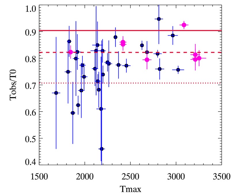
Figure 16: Figure 7 of Cowan and Agol (2011) replotted with the 36 hot Jupiters analyzed in this paper. WASP-14b, -19b, and -103b are represented by two eclipses each (as per Table 1), so there are 39 total points. $T_{obs}$ is our observed day side temperature, from the error-weighted average of the 3.6- and 4.5 $\mu$m brightness temperatures. $T_{0}$ is the equilibrium temperature that would result at the sub-stellar point with zero albedo, in the limit of no redistribution of heat. $T_{max}$ is the calculated day side equilibrium temperature with zero albedo and no redistribution of heat. Just as in their original figure, the solid line shows zero recirculation, the dashed line is a uniform day-hemisphere, and the dotted line is a uniform planet. An albedo of zero was used to calculate the red lines. Planets with published Spitzer phase curves are plotted in magenta, but using values from our eclipse results.

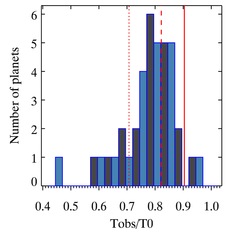
Figure 17: Histogram of $T_{obs}/{T_{0}}$ values from the Y-axis of Figure 16. $T_{obs}$ is our observed day side temperature, from the error-weighted average of the 3.6- and 4.5 $\mu$m brightness temperatures. $T_{0}$ is the equilibrium temperature that would result at the sub-stellar point with zero albedo, in the limit of no lateral redistribution of heat. Alternate colors for adjacent histogram bins are used solely for visual clarity. As in Figure 16, the solid red line shows zero heat redistribution, the dashed line is a uniform day-hemisphere, and the dotted red line is a uniform planet. The median value of $T_{obs}/{T_{0}}$ is 0.79 for our sample, very close to uniform day-side hemispheres. An albedo of zero was used to calculate the red lines. Planets falling left of the dotted red line must have albedos significantly greater than zero.

7 Implications for Emergent Spectra and Atmospheres

We now discuss the implications of our secondary eclipse depths for the emergent spectra of hot Jupiters, and for physical conditions in their atmospheres. As prelude to the results, we first explain the rationale for a statistical approach (Sec. 7.1), and we describe two sets of modeled spectra that we use in this study (Sec. 7.2). Our results for the planets (Secs. 7.3 to  7.5) differ from expectations based on classic 1-D model atmospheres, and in Sec. 7.6 we discuss that difference in terms of the atmospheric structure of the planets.

7.1 A Statistical Approach

The earliest results for Spitzer’s secondary eclipses of hot Jupiters were interpreted in terms of molecular absorptions (e.g., Madhusudhan et al., 2011). Hansen et al. (2014) questioned whether molecular features can be reliably detected using Spitzer’s photometry. Figure 18 shows an example of fitting eclipse depths in those two channels to a blackbody planet. This fit yields a good estimate for the day side temperature of the planet. However, due to modest signal-to-noise and the lack of molecular band shape information, it is not typically possible to confidently associate molecular features with deviations from the best-fit blackbody.

Rather than attempting to identify molecular absorptions in individual planets, we adopt a statistical approach wherein we look for trends in our total sample. Pioneering work of this type was reported by Triaud (2014a); Triaud et al. (2014b); Beatty et al. (2014, 2019), and also Kammer et al. (2015), Adams & Laughlin (2018), and Wallack et al. (2018). A statistical approach to transit (not eclipse) spectroscopy was elucidated by Sing et al. (2016). Our statistical approach differs somewhat from past work, as we explain in Sec. 7.3.

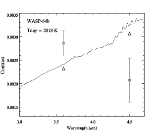
Figure 18: Example of fitting 3.6- and 4.5 $\mu$m eclipse depths to a blackbody planet, with an ATLAS model atmosphere to represent the star. The squares with error bars are the observed eclipse depths, and the triangles are the values expected from integrating models of the planet and star over the Spitzer bandpasses, using the IRAC response functions. WASP-64b has an equilibrium temperature of 1674K, assuming zero albedo and redistribution uniformly over both the day and night hemispheres. The best-fit blackbody has a temperature of 2018K, consistent with less than uniform redistribution (as per Figure 16). The ripples in the best-fit curve are due to spectral structure in the modeled stellar spectrum.

7.2 Two Sets of Models

We use two sets of well documented model atmospheres for the planets, from Adam Burrows (Burrows et al., 1997, 2006) and Jonathan Fortney (Fortney et al., 2005, 2008). Rather than calculating individual models for each of the 36 hot Jupiters in our sample, we model the planets using ’tracks’ wherein the stellar insolation varies in magnitude. We adopt stellar and planetary mass and radius based on the median values of our sample, thereby making an average hot Jupiter orbiting an average star. We vary the planetary temperature by placing that average planet at different orbital distances, and we use solar metallicity cloudless atmospheres for all models. The Burrows and Fortney codes use different treatments of heat redistribution: Fortney adopts a uniform redistribution over both day and night hemispheres, whereas Burrows redistributes approximately over the day hemisphere, and partially into the night hemisphere. The consequence is that the Fortney models are cooler than the Burrows models at a given orbital distance. But a Fortney model at an orbital distance of $a/\sqrt{2}$ should produce a comparable spectrum to a Burrows model orbiting at distance $a$; in particular it will have a very similar day side effective temperature (total energy re-radiated). That comparison is shown in Figure 19.

The two spectra in Figure 19 indeed have close overall flux levels, and spectral features that correspond in relative strength and shape versus wavelength, but not in total amplitude. The Burrows models have overall deeper absorption features than the Fortney models at the same effective temperature. The reason for that difference is not obvious, due to the complexity of the models. A myriad of possible differences can come into play, and fully exploring the underlying physics is beyond the scope of this paper. As one example, the different treatments of longitudinal heat redistribution can also affect the vertical temperature structure, and different temperature structures as a function of optical depth will produce different emergent spectra. Fortunately, our principal result is not affected by the differences between the two sets of models, as we discuss in Sec. 7.3. Also, we find that the two sets of models produce tracks that conveniently bracket the observed locus of the planets. We thereby use the models to gauge the average magnitude of absorption features in the exoplanetary spectra (Sec. 7.3).

We also utilize both Burrows and Fortney models that feature temperature inversions. The Burrows inverted models were computed by adding extra absorbing opacity between 0.003 and 0.6 bars, and preserving flux-constancy. The inverted Fortney models simply specified temperature to increase linearly with decreasing log of pressure below one bar ($dT/d\log{P}=-160$K). Those models are not flux-constant, but we use them only to explore how the inverted profiles affect the relative brightness temperature of the planets in the two Spitzer bands (Sec. 7.6).

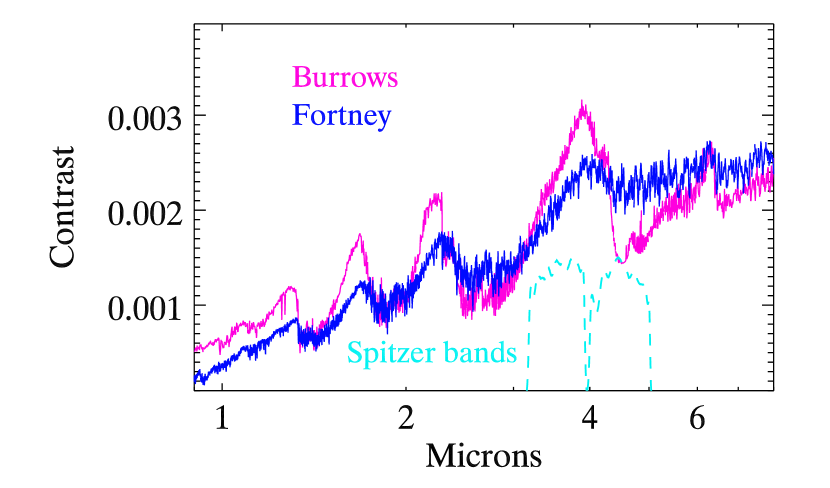
Figure 19: Comparison of Burrows and Fortney modeled spectra for planetary and stellar parameters equal to our average host star, and average planet. Those parameters are $T_{s}=6040$K, $R_{s}=1.4R_{\odot}$, $R_{p}=1.4R_{J}$, and $M_{p}=1.5M_{J}$. The Burrows model lies at an orbital distance of 0.025 AU, versus 0.018 AU for the Fortney model. Their day side temperatures are closely similar, due to different prescriptions for redistribution of stellar irradiance (see text, Sec. 7.2). The Burrows model has stronger spectral features, as discussed in Sec. 7.2. The Spitzer band response functions at 3.6- and 4.5 $\mu$m are included for comparison.

7.3 Deviations from Blackbody Spectra

Several statistical treatments have examined Spitzer colors of hot Jupiters versus their brightness in a particular band (i.e, an HR-diagram analogy). That approach is particularly useful when the luminosity of the planet is produced by an internal source. But hot Jupiters primarily re-radiate external energy from their star, and their emergent spectrum is determined to first order by the level of irradiance. In this case we find it useful to relate the planetary brightness temperatures in the two Spitzer bands, rather than to correlate color with total brightness. In other words, we want to study the shape of the emergent spectrum, not the total luminosity of the planet.

Figure 20 shows the brightness temperature of our planets at 4.5 $\mu$m versus their 3.6 $\mu$m brightness temperature. The model tracks from Burrows and Fortney are included, and the relation for purely blackbody planets ($T_{4.5}=T_{3.6}$) is shown as a dotted blue line. In general, the Fortney model track passes through the envelope of the observed planets, and the Burrows track lies at the lower envelope (we quantify those statements below). The 4.5 $\mu$m Spitzer band contains strong opacity from both water vapor and carbon monoxide, that is especially manifest in the Burrows spectra compared to Fortney (see Figure 19). That causes the Burrows models to have a lower 4.5 $\mu$m brightness temperature than Fortney, and thereby the Burrows track lies lower. The 4.5 $\mu$m band is thus indicative of overall stronger absorptions in the Burrows models versus Fortney (as per Figure 19), and we find that difference to be very useful as a diagnostic of the spectra of the planets. Most (60%) of the observed planets lie between the two model tracks, indicating that the amplitudes of their spectral absorptions (especially at 4.5 $\mu$m) are intermediate between the Burrows and Fortney models. That is an interesting inference, because to date there is little information on the magnitude of spectral features that applies to a comparably large sample of hot Jupiters.

We quantify the differences between the observed planets and the model tracks by fitting a straight line to the 4.5- versus 3.6 $\mu$m brightness temperature measurements, using the maximum likelihood method of Kelly (2007). From the precision on the intercept of that line, we find that the Fortney inverted track is $2.6\sigma$ higher than the average of the observations (not surprising, since temperature inversions have been found for only a few hot Jupiters). The Fortney ’normal’ models agree well with the observations (being only $0.04\sigma$ higher), and the Burrows track is $11\sigma$ below the observations, reflecting the strong modeled absorption in CO (Figure 19). The slope of the fitted line is greater than unity ($1.085\pm 0.040$, $2.1\sigma$ above unity). Although that slightly steeper-than-unity slope is not statistically secure, it is suggestive, especially because there have been previous hints of that effect. Kammer et al. (2015) and Wallack et al. (2018) found that cool Jupiters ($T<1200$K) tend to have lower brightness temperatures at 4.5 $\mu$m than at 3.6 $\mu$m. Beatty et al. (2019) examined brightness temperatures in the two Spitzer bands as a function of equilibrium temperature for hot Jupiters with phase curves, and their data suggest (but do not prove) a greater slope at 4.5- versus 3.6 $\mu$m, consistent with our Figure 20. Beyond hot Jupiters, it has long been known that the exo-Neptune GJ 436b ($T\sim 800$K) exhibits a puzzling flux excess at 3.6 $\mu$m, that was attributed to disequilibrium chemistry (Stevenson et al., 2010), and a similar effect was recently found in GJ 3470b (Benneke et al., 2019). We hypothesize that Figure 20 hints at a pervasive and general effect that occurs over a large range of equilibrium temperature, and we investigate further using a physically somewhat different relation: the ratio of 4.5- to 3.6 $\mu$m brightness temperature as a function of equilibrium temperature.

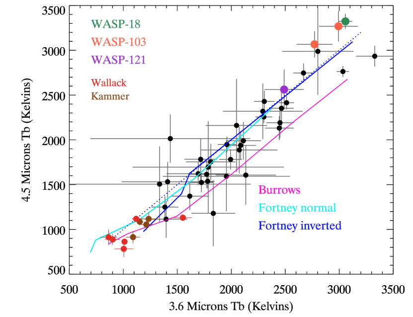
Figure 20: Comparison of brightness temperatures in both Spitzer bands. Blackbody planets would fall along the dotted blue line which has a slope of unity. Tracks of models from Burrows and Fortney are shown, and the inverted Fortney track merges with the normal track at high temperature (see text, Sec. 7.6), and the inverted Burrows track (not illustrated) does also. The observations indicate that the planets are close to blackbodies, but cooler planets tend to have lower brightness temperatures at 4.5 $\mu$m compared to 3.6 $\mu$m, whereas hotter planets tend to be brighter at 4.5 $\mu$m compared to 3.6 $\mu$m. Brightness temperatures from Kammer et al. (2015) and Wallack et al. (2018) are included in order to enhance the comparison for the coolest planets observed in secondary eclipse. The planets from Kammer et al. (2015) are HAT-19b, WASP-6b, -10b, and -39b. The planets added from Wallack et al. (2018) are HAT-12b, -18b, -20b, and WASP-8b, -69b, and 80b. See Sec. 7.3 and Sec. 7.4 for discussion.

7.4 A Slope in Brightness Temperaure Ratio

If indeed the 4.5 $\mu$m versus 3.6 $\mu$m brightness temperature relation has a slope that exceeds unity, then the ratio of those brightness temperatures should be an increasing function of the equilibrium temperature of the planets, whereas the ratio would be constant (slope equal to zero) for blackbody planets. The observed relation (including the planets from Kammer et al., 2015 and Wallack et al., 2018) is shown in Figure 21, and a maximum-likelihood regression yields a slope of $100\pm 24$ parts-per-million (ppm) per Kelvin. That slope is significant at $4.1\sigma$, and is obvious on Figure 21. We confirmed the statistical significance using a nonparametric (Kendall-Tau) test. Kendall-Tau rejects the null hypothesis of uncorrelated data with a p-value of 0.0012. For each 1K increase in equilibrium temperature, the ratio of brightness temperatures (4.5 to 3.6) increases by 0.01%. Thus, from 800K to 2500K (for example), the ratio increases by 0.17, as shown by the red line on Figure 21.

We repeated the maximum-likelihood slope solution by omitting the planets from Kammer et al. (2015) and Wallack et al. (2018). That solution gives a slope of $152\pm 49$ ppm per Kelvin, still significant at $3.1\sigma$. We also repeated the solution using our set of GC eclipse depths (Section 3.4, but including Kammer et al., 2015 and Wallack et al., 2018), and that decreases the slope to $87\pm 26$ ppm per Kelvin, still significant at $3.3\sigma$. As a third possible case, we use our set of PD eclipse depths (also described in Section 3.4), and the slope is $105\pm 24$ ppm per Kelvin, significant at $4.4\sigma$. We also explored to what effect the significance of the result depends on the size of the per-point error bars. Increasing the size of the per-point error bars by the (arbitrary, but implausible) factor of 1.5 (including the planets from Kammer et al. (2015) and Wallack et al., 2018), decreases the significance of the slope, but only to $3.1\sigma$. Considering also that the Kendall-Tau test is independent of the error bars, we conclude that the observed planets robustly deviate from the blackbody line in the sense that hotter planets tend to become more prominent at 4.5 $\mu$m relative to 3.6 $\mu$m.

A corollary of our conclusion is that the planets also robustly deviate from the model tracks, not merely from blackbodies. Specifically, the normal Fortney track has a slope of +19 ppm per Kelvin (in Tb(4.5)/Tb(3.6) vs. $T_{eq}$) for $T>1000$K (versus the observed slope of $100\pm 24$ ppm per Kelvin), and the modeled ratio increases sharply to $>1.1$ for $T<1000$K, due to methane absorption in the 3.6 $\mu$m band, very unlike the observations.

We also investigated whether the Tb(4.5)/Tb(3.6) ratio correlates with stellar host temperature, and we find a $2.2\sigma$ effect. However, planetary equilibrium temperature is a function of stellar temperature, so we would expect some degree of correlation with stellar temperature as a by-product of the correlation with planetary equilibrium temperature. The stronger correlation of Tb(4.5)/Tb(3.6) with planetary equilibrium temperature indicates that the the temperature of the host star per se is not a primary factor.

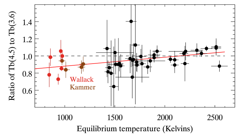
Figure 21: Ratio of the 4.5- to 3.6 $\mu$m brightness temperature for our planets, plus planets from Kammer et al. (2015) and Wallack et al. (2018). The brightness temperature ratio is shown versus exoplanetary equilibrium temperature. The ratio would be constant at unity for blackbody planets (dashed line), but a maximum likelihood regression (Kelly, 2007) indicates an upward slope (red line), significant at $4.1\sigma$.

7.5 A Selection Effect?

We first consider whether the slope on Figure 21 could be due to a selection effect. Eclipses in Spitzer’s 3.6 $\mu$m band are harder to detect than at 4.5 $\mu$m. If the cooler planets have undetectable 3.6 $\mu$m brightness temperatures, then the sample will tend to be incomplete for cool planets with high brightness temperature ratios (4.5 divided by 3.6). That will bias the slope in the direction that we observe. To evaluate whether this is a significant effect, we add five planets that are not currently included on Figure 21 because their eclipses were too weak to measure at 3.6 $\mu$m. Those are WASP-75b and -49b (Figure 22), WASP-67b from Kammer et al. (2015), and HAT-P-26b (and -17b at 4.5 $\mu$m) from Wallack et al. (2018). For each of those planets, we postulate a 3.6 $\mu$m eclipse depth that equals twice the error of the fit, a $2\sigma$ ’detection’. Using a hypothetically minimal detection is conservative in this context, because it will maximize the brightness temperature ratio, while remaining consistent with the fact that the eclipses are not detected. Adding those five planets, the significance of the slope on Figure 21 indeed decreases, but only from $4.1\sigma$ to $3.9\sigma$. We conclude that a selection effect is not sufficiently strong to produce the slope that we observe, and we turn to possible astrophysical explanations.

7.6 Atmospheric Temperature Structure

Since the emergent flux from exoplanetary atmospheres is directly related to the atmospheric source function (= the Planck function in LTE), it is virtually axiomatic that the slope we observe is related to the temperature structure of the atmospheres (i.e., temperature versus optical depth). A prominent type of perturbation to exoplanetary atmospheric structure is the possible presence of temperature inversions. Inversions have a long and popular history in exoplanetary science (e.g., Hubeny et al., 2003; Knutson et al., 2008, 2009; Nymeyer et al., 2011; Haynes et al., 2015; Beatty et al., 2017; Sheppard et al., 2017; Arcangeli et al., 2018; Kreidberg et al., 2018; Mansfield et al., 2018). Spitzer’s 4.5 $\mu$m band is formed high in the atmosphere (Burrows et al., 2007), so an atmospheric temperature rising with height can in principle produce an excess brightness temperature at 4.5 $\mu$m relative to 3.6 $\mu$m. Strong stellar irradiance provides the energy to maintain inversions, so a ratio of brightness temperatures (4.5 to 3.6) that increases with equilibrium temperature (as we observe) is at least qualitatively consistent with temperature inversions. Nevertheless, we do not conclude that temperature inversions are the dominant effect that we are observing in Figure 21. Instead, we believe that the dominant effect is more subtle and pervasive than the temperature inversion phenomenon, as we now discuss.

Since Spitzer’s 4.5 $\mu$m band contains both strong water vapor opacity, and the strong 1-0 band of carbon monoxide, it is indeed sensitive to high altitude temperature inversions. Three planets in our sample (WASP-18b, -103b, and -121b) have been reported as hosting inversions (Nymeyer et al., 2011; Sheppard et al., 2017; Arcangeli et al., 2018; Kreidberg et al., 2018; Evans et al., 2017). Those three planets are highlighted on Figure 20, and they tend to lie at the upper envelope with a high 4.5 $\mu$m brightness temperature, albeit they are not decisively separated from the remainder of the sample. However, the contribution functions of the 3.6- and 4.5 $\mu$m bands are often overlapping (see Figure 12 of Kreidberg et al., 2018), so temperature inversions will tend to raise both the 3.6- and 4.5 $\mu$m brightness temperatures. In the case where the inversion extends over a broad range of pressure, planets will tend to move along the model track, rather than perpendicular to it. The inverted Fortney model track illustrates this point: at high temperature it merges with the track for non-inverted models, but a given planet lies at a lower or higher position on the track depending on whether the temperature gradient is normal or inverted. In order to move planets above and away from the model track (significantly brighter at 4.5 $\mu$m), it is necessary to ’fine tune’ the temperature inversion to affect the 4.5 $\mu$m contribution function, while minimizing the impact on the 3.6 $\mu$m contribution function.

We cannot exclude the possibility that multiple mechanisms are at play when accounting for our results. One possibility is Burrows-like strong absorption (see Sec. 7.3) for planets with equilibrium temperatures below $\sim 2000K$, coupled with blackbody-like behavior for the hottest planets due to the water dissociation and chemistry/opacity issues discussed by Parmentier et al. (2018b) and Lothringer et al. (2018). Another possibility is a metallicity effect that comes into play at low temperature as discussed by Kammer et al. (2015), as well as possible temperature inversions for the hottest planets. Also, emission in CO due to mass loss (Bell et al., 2019) could increase Tb(4.5) for the most strongly irradiated planets. However, we prefer the simplicity of a single hypothesis to account for the total effect that we observe. As regards temperature inversions, we do not think they play a major role in our results, for several reasons: 1) Inversions have to be fine-tuned to raise planets relative to the model track, 2) the three nominally inverted planets on Figure 20 are not significantly separated from the rest of the sample, and 3) inversions are unlikely to be sufficiently prevalent to affect the brightness temperature ratio over the large range of temperature illustrated on Figure 21.

We point out that Spitzer’s Tb(4.5) measurement can be a significant factor driving retrievals toward an atmospheric temperature inversion (e.g., for WASP-18b, Nymeyer et al., 2011; Sheppard et al., 2017). Given a systematic tendency for hotter planets to be relatively brighter than the models at 4.5 $\mu$m, together with random noise, some of the hottest planets may then reach a threshold where the retrieval codes react by requiring a temperature inversion for planets at the upper end of the distribution in Tb(4.5). Our ’big picture’ data suggest that the primary difference between the models and the real planets is systematic over a large range of temperature, rather than inversions in some of the hottest planets.

We suggest that Figure 21 requires a pervasive difference between the models and the real planets, systematically affecting the temperature versus optical depth structure as a function of equilibrium temperature. One possibility is a difference in opacities between the planets and the models. Another possibility is the effect of a vigorous zonal circulation on the radial temperature gradient (i.e., 3-D versus 1-D models) is one possibility. In that respect, the greater efficiency of heat redistribution on cooler versus hotter planets (Figure 16) is potentially an important factor. Other possibilities include systematic changes in haze opacity (particle size, composition, and height) as a function of equilibrium temperature, and height gradients in the relative mixing ratios of CO and water vapor (chemical equilibrium, or not). The physics underlying this systematic trend can hopefully be clarified using spectroscopy by JWST.

8 Summary

In this paper we have investigated the emergent spectra of transiting hot Jupiters, using their secondary eclipses as observed in the two warm Spitzer bands at 3.6- and 4.5 $\mu$m. We report eclipse depths for twenty seven previously unobserved planets, and we re-analyze eclipses of 9 previously observed planets in order to compare and relate our results to published work. Our new planets include highly irradiated worlds such as KELT-7b, WASP-87b, WASP-76b, and WASP-64b, as well as others that are important targets for JWST, such as WASP-62b. We also analyze Spitzer transits of KELT-7, WASP-62, and WASP-74, in order to improve the precision of their orbital periods (Section 3.1). Our Spitzer eclipse fits (Section 3.2) utilize photometry extracted using four different methods (Section 2), each with multiple aperture sizes, and a pixel-level decorrelation method to correct instrumental effects and thereby select the optimum values of eclipse depth. We investigate and discuss the statistical properties of our fitted eclipse depths (Section 3.4), including a comparison to the magnitude of the photon noise, analysis of the Allan deviation slope, and comparison to eclipse depths for the 9 planets previously published.

The orbital phase of a secondary eclipse is sensitive to non-zero orbital eccentricities, and we investigate those phases for our sample of planets (Section 4). We find statistical evidence that eclipses tend to increasingly deviate from phase 0.5, the deviation increasing with orbital period in the range of our sample (periods 0.8 to 5.3 days), indicating an increasing lack of orbital circularization. We conclusively find a slightly eccentric orbit for WASP-62b ($e\cos{\omega}=0.00614\pm{0.00064}$, Section 4), that lies in the continuous viewing zone of JWST. The eclipse of that planet occurs about 23 minutes later than orbital phase 0.5, and that delay is significant for planning of JWST observations. Even for circular orbits, the phase of secondary eclipse is predicted to be offset from 0.5 due to temperature structure on the exoplanetary disk (Williams et al., 2006). Excluding planets with notably eccentric orbits, our sample has an average eclipse phase over both Spitzer wavelengths that is centered on 0.5 to a precision of about $\pm 23$ seconds. We do not detect a time offset because our precision is comparable to the offset predicted by Williams et al. (2006), but we do exclude some of the larger values that they modeled. Our precision on the average eclipse phase of our sample is modestly poorer than the offset successfully measured for HD 189733b by Agol et al. (2010). We project that a complete sample of Spitzer eclipses (all planets observed), especially with improved precision in their orbital ephemerides, would be sufficient to detect the offset for the ’average planet’, thereby extending the result from Agol et al. (2010) to the larger sample.

We apply corrections for dilution of eclipse depths by stellar companions to some systems (Sec. 3.5), and then convert the eclipse depths to brightness temperatures in each Spitzer band (Section 5), using ATLAS model atmospheres for the host stars (Kurucz, 1979). We use those brightness temperatures to investigate heat redistribution on the day sides of the planets (Section 6), following the approach of Cowan and Agol (2011). We find that planets whose calculated maximum day size temperature exceeds $\sim 2200$K are well described by an observed brightness temperature consistent with zero albedo and redistribution of stellar irradiance uniformly over the day side. About 35% of planets whose calculated maximum temperature falls between $\sim\,1700$K and $\sim\,2200$K require non-zero albedos, even if their redistribution of stellar irradiance is uniform over the entire planet. Six planets in our sample have published Spitzer phase curves, and these planets are typical of the entire sample, and consistent with uniform redistribution of stellar irradiance over the day side.

To investigate the emergent day side spectra of our planets, we invoke a statistical approach whereby we compare brightness temperatures in the two Spitzer bands, and seek trends for the entire sample (Section 7.1). We compare the observed brightness temperatures (Tb) to two sets of well documented model atmospheres, from Adam Burrows and Jonathan Fortney (Section 7.2), both based on cloudless atmospheres with solar abundances. Those models differ in the amplitude of their absorption features due to differences in their temperature structures, with the Burrows models predicting stronger absorptions than the Fortney models. We also compare the observed brightness temperatures to blackbody planets (Section 7.3), for which the day side brightness temperatures would be equal in the two Spitzer bands. In the Tb(4.5) versus Tb(3.6) plane, the observed planets seem to slope more steeply than a blackbody, with the hottest planets being brighter at 4.5 relative to 3.6, and the cooler planets being fainter at 4.5 relative to 3.6. While that tendency is not statistically secure, it did motivate us to investigate a similar trend, that we find to be robust (see below).

Comparing the observed brightness temperatures to models, we find that the Burrows and Fortney models bracket 60% of the observed planets in Tb(4.5), with the Fortney models lying near the center in Tb(4.5), and the Burrows models at the lower envelope. Because molecular absorptions are stronger in the 4.5 $\mu$m band than at 3.6 $\mu$m, that bracketing thereby constrains the average amplitude of absorption features in the day side spectra of our planets.

Our most intriguing result is that the ratio of Tb(4.5) to Tb(3.6) increases with equilibrium temperature, and we show that this trend is statistically significant (Section 7.4), and is not due to selection effects (Section 7.5). Adding lower temperature planets (800 to 1200K) from Kammer et al. (2015) and Wallack et al. (2018), we find that the ratio of Tb(4.5) to Tb(3.6) increases by 100$\pm 24$ ppm for each 1K increase in equilibrium temperature from 800K to 2500K. No existing model predicts this trend over such a large range of temperature. While it could in principle be due to a combination of effects such as temperature inversions in the hotter planets of the sample, coupled with stronger-than-modeled molecular absorption for the cooler planets, we advance the simple hypothesis (Section 7.6) that it represents a structural difference in the atmospheric temperature profile between the real planetary atmospheres compared to models.

9 Acknowledgements

We thank the staff of the Spitzer Space Telescope for their help in planning, and their careful scheduling and execution of the observations. We also thank an anonymous referee and the statistical editor for comments that significantly improved this paper. This work was supported by NASA ADAP grant NNX16AF34G.

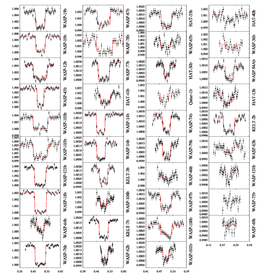
Figure 22: Eclipses at 3.6 $\mu$m for all hot Jupiters analyzed in this paper. The abscissa for all plots is orbital phase and the ordinate is relative flux. The eclipses are sorted by deepest to shallowest eclipse depth, going top to bottom and left to right. The data are binned for clarity, with between 20 and 40 points per dataset. The fitted eclipse is overplotted in red. The error bars are the scatter in each individual bin. The planet names are to the right of each plot. Note that the x-axis scale changes between columns and y-axis scale changes between each eclipse. All eclipses are nominally detected (i.e., they have positive depths near the expected phase), except for WASP-75b and -49b (lowest right), where negative eclipse depths are derived. Considering the planets with positive eclipses, the ratio of eclipse depth to its random error varies from 1.6 (WASP-36) to 48 (WASP-18), and the median is 15.

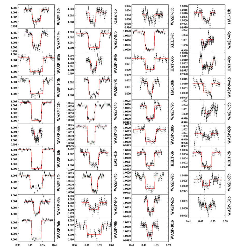
Figure 23: Eclipses at 4.5 $\mu$m for all hot Jupiters analyzed in this paper, similar to the 3.6 $\mu$m eclipses shown in Figure 22. All eclipses are nominally detected, and the ratio of eclipse depth to its random error varies from 1.1 (WASP-75) to 41 (WASP-18), and the median is 12.

Table 1: Eclipse depths (ED) in contrast units of parts-per-million, normalized to the flux from the host star. These are ’as observed’, without dilution corrections applied. Dilution correction factors are given in Table 4. The type of fit to the photometry is encoded as: temporal baseline (L=linear, Q=quadratic, E=exponential), centroiding method (C=center of light, G=2-D Gaussian fit), photometric aperture type (F=fixed radii, V= variable, using the noise-pixel formulation), and the number of minutes trimmed from the start of the observations. For example LGF30 means a linear baseline, Gaussian centroiding, fixed radius aperture, and 30 minutes trimmed from the start of the observations. The ’bin’ column lists the bin size used in the PLD solutions (see text). ’Ratio’ is the ratio of scatter in the unbinned residuals, divided by the photon noise. ’Slope’ is the slope of the relation between the log of standard deviation of the residuals using multiple bin sizes, versus the square root of the bin size. The AOR is the Astronomical Observation Request number that uniquely identifies the data we used from the Spitzer Heritage Archive.

Planet Name	AOR	3.6 ED (ppm)	Fit Type	Bin	Ratio	Slope	AOR	4.5 ED (ppm)	Fit Type	Bin	Ratio	Slope
HAT-13	38808320	851$\pm$107	ECV30	120	1.28	-0.42	38808832	1090$\pm$124	LCF30	96	1.17	-0.50
HAT-30	42612736	1584$\pm$107	LCV60	28	1.11	-0.45	42613504	1762$\pm$147	LCF60	16	1.21	-0.45
HAT-33	62151424	1603$\pm$127	QGF45	18	1.15	-0.47	51838720	1835$\pm$199	LCF45	1344	1.25	-0.48
HAT-40	51832064	988$\pm$168	LGF30	544	1.30	-0.40	62151936	1057$\pm$145	LGF30	2	1.08	-0.51
HAT-41	51840512	1829$\pm$319	QGF30	512	1.23	-0.39	51838464	2278$\pm$177	LGF30	640	1.20	-0.45
KELT-2	51835136	650$\pm$ 38	QGV30	34	1.11	-0.40	51833600	678$\pm$ 47	QGV30	26	1.09	-0.49
KELT-3	51815936	1766$\pm$ 97	LGF30	480	1.28	-0.40	51842048	1656$\pm$104	LGF30	320	1.16	-0.45
KELT-7	62154496	1688$\pm$ 46	QGV30	34	1.05	-0.43	62155520	1896$\pm$ 57	QGF30	46	1.12	-0.46
Qatar-1	51819776	1511$\pm$455	LGF45	336	1.36	-0.49	51816960	2907$\pm$415	LGF0	544	1.58	-0.49
WASP-12	48014848	4247$\pm$243	QGF30	28	1.15	-0.40	48015872	3996$\pm$171	LCF30	10	1.21	-0.46
WASP-14	45426944	1816$\pm$ 67	QCV30	60	1.10	-0.46	45426688	2161$\pm$ 88	QCF30	12	1.19	-0.43
WASP-14	45427968	1798$\pm$ 59	LCV30	8	1.11	-0.49	45428992	2284$\pm$ 90	QCF30	54	1.19	-0.40
WASP-18	38805760	3037$\pm$ 62	QCF30	24	1.10	-0.46	40269312	4033$\pm$ 97	QCF30	26	1.10	-0.49
WASP-19	43970048	5016$\pm$259	QCV30	120	1.31	-0.49	43970560	5081$\pm$392	QGF30	6	1.17	-0.48
WASP-19	43970048	5070$\pm$233	QCF30	4	1.14	-0.53	43970560	5848$\pm$544	QGF30	108	1.17	-0.48
WASP-36	51829504	913$\pm$578	LGF30	18	1.25	-0.47	51827456	1948$\pm$544	LGF30	62	1.16	-0.51
WASP-43	42614272	3773$\pm$138	QGV30	32	1.22	-0.45	42615040	3866$\pm$195	LCF30	14	1.23	-0.45
WASP-46	51823872	1360$\pm$701	LGF30	50	1.38	-0.49	51821568	4446$\pm$589	LGV30	92	1.34	-0.54
WASP-49	51828480	-189$\pm$265	LCF60	184	1.21	-0.40	51826688	1073$\pm$336	LCF60	304	1.22	-0.51
WASP-62	51823360	1616$\pm$146	QGF45	352	1.16	-0.46	51821056	1359$\pm$130	QGF45	448	1.15	-0.47
WASP-63	51835904	486$\pm$ 96	LGF30	42	1.23	-0.43	51834112	560$\pm$130	LGF30	1024	1.18	-0.50
WASP-64	51816704	2859$\pm$270	LGF30	18	1.24	-0.44	51842560	2071$\pm$471	LGF30	108	1.16	-0.48
WASP-65	51828224	1587$\pm$245	LGV30	2	1.67	-0.40	51826432	724$\pm$318	LGV30	2	1.56	-0.46
WASP-74	62170880	1446$\pm$ 66	LGV30	34	1.07	-0.44	62171904	2075$\pm$100	LGF30	136	1.10	-0.50
WASP-75	51826176	-86$\pm$290	QCV	2	1.44	-0.44	51824384	452$\pm$399	LCF0	168	1.29	-0.49
WASP-76	58239232	2597$\pm$ 63	QGF30	18	1.11	-0.43	58238720	3344$\pm$ 82	QCF30	96	1.11	-0.48
WASP-77	51820544	1845$\pm$ 94	QGF30	4	1.19	-0.46	51818496	2362$\pm$127	QGF30	40	1.20	-0.47
WASP-78	51833088	2001$\pm$218	LGV30	80	1.54	-0.45	51830528	2013$\pm$351	QGF30	168	1.14	-0.49
WASP-79	51841536	1394$\pm$ 88	LCF60	64	1.19	-0.41	51839488	1783$\pm$106	LCF60	288	1.15	-0.48
WASP-87	62173952	2077$\pm$127	LCV45	88	1.10	-0.45	62174464	2705$\pm$137	LGF45	8	1.21	-0.49
WASP-94A	62174976	867$\pm$ 59	LCV30	10	1.16	-0.42	62176000	995$\pm$ 93	LGF30	12	1.23	-0.42
WASP-97	62177024	1359$\pm$ 84	QCV30	4	1.09	-0.48	62177536	1534$\pm$101	LCF30	12	1.12	-0.46
WASP-100	62156544	1267$\pm$ 98	LGF30	30	1.19	-0.40	62157056	1720$\pm$119	LGF30	18	1.13	-0.46
WASP-101	62157568	1161$\pm$111	LGV30	8	1.26	-0.43	62158592	1194$\pm$113	LGV30	10	1.13	-0.47
WASP-103	53518080	3294$\pm$193	LGV30	4	1.13	-0.50	53513472	4552$\pm$369	QCF30	14	1.14	-0.47
WASP-103	53519104	3350$\pm$218	QCV30	4	1.26	-0.51	53514240	4711$\pm$339	QCF30	8	1.12	-0.47
WASP-104	62179584	1709$\pm$195	LGF30	18	1.27	-0.45	62180864	2643$\pm$303	QGF30	12	1.18	-0.47
WASP-121	62159616	3685$\pm$114	QCV30	26	1.08	-0.50	62160640	4684$\pm$121	LCF30	12	1.11	-0.48
WASP-131	62162688	364$\pm$ 96	QCV30	68	1.16	-0.45	62163712	289$\pm$ 80	LCF30	8	1.16	-0.42

Table 2: Transit times in BJD(TDB), transit depths, and updated orbital periods for KELT-7b, WASP-62b, and WASP-74b, based on the transits discussed in Section 3.1. The values of $T_{0}$ for all three planets are repeated from Bieryla et al. (2015), Hellier et al. (2012), and Hellier et al. (2015), but converted to TDB as needed.

Planet	3.6 $\mu$m time	4.5 $\mu$ time	$T_{0}$ BJD(TDB)	Period (days)
KELT-7b	$2457749.95953\pm{0.00016}$	$2457758.16446\pm{0.00019}$	$2456355.229809\pm{0.000198}$	$2.73476468\pm{0.00000046}$
WASP-62b	$2457717.23121\pm{0.00021}$	$2457730.46660\pm{0.00024}$	$2455855.39272\pm{0.00027}$	$4.41193897\pm{0.00000074}$
WASP-74b	$2457768.16637\pm{0.00024}$	$2457770.30472\pm{0.00029}$	$2456506.8926\pm{0.0002}$	$2.13775257\pm{0.00000046}$

Table 3: Spitzer transit depths ($R_{p}^{2}/R_{s}^{2}$, in ppm) for KELT-7b, WASP-62b, and WASP-74b.

Planet	3.6 $\mu$m	4.5 $\mu$m
KELT-7b	7925$\pm$62	8092$\pm$36
WASP-62b	12189$\pm$101	12250$\pm$87
WASP-74b	9044$\pm$56	9197$\pm$43

Table 4: Dilution corrections for secondary eclipse depth at both Spitzer wavelengths. The ”as measured” eclipse depths listed in Table 1 were multiplied by these factors before they were used in the analyses reported in Sec. 7, and for the brightness temperatures listed in Table 6.

Planet	3.6 $\mu$m factor	4.5 $\mu$m factor
HAT-P-30b	1.0121	1.0117
HAT-P-33b	1.0377	1.0332
HAT-P-41b	1.0069	1.0111
KELT-2b	1.137	1.123
KELT-3b	1.0125	1.0127
WASP-12b	1.1101	1.0983
WASP-36b	1.0015	1.0026
WASP-49b	1.0130	1.0124
WASP-76b	1.1470	1.1250
WASP-77b	1.0929	1.0530
WASP-87b	1.0014	1.0011
WASP-103b	1.1700	1.1490

Table 5: Central phases and times of the secondary eclipses. The ephemeris source column gives the reference used to calculate the orbital phase from the BJD(TDB) times. The phases are ’as observed’ and have not been corrected for light travel time across the orbit. The errors in eclipse phase are purely due to the eclipse observations and do not include imprecision in the orbital ephemeris. Note that our analysis in Sec. 4 does include uncertainty in the orbital ephemeris when analyzing the properties of the eclipse phases.

Planet	3.6 $\mu$m Phase	3.6 $\mu$m BJD(TDB)	4.5 $\mu$m Phase	4.5 $\mu$m BJD(TDB)	Ephemeris source
HAT-13	0.49378 $\pm$ 0.00120	55326.70691 $\pm$ 0.00351	0.49495 $\pm$ 0.00110	55355.87271 $\pm$ 0.00319	Southworth+2012
HAT-30	0.50284 $\pm$ 0.00073	55930.06169 $\pm$ 0.00205	0.50068 $\pm$ 0.00086	55944.10866 $\pm$ 0.00243	Maciejewski+2016
HAT-33	0.50109 $\pm$ 0.00070	57784.53823 $\pm$ 0.00243	0.50025 $\pm$ 0.00144	57027.10001 $\pm$ 0.00501	Hartman+2011
HAT-40	0.49829 $\pm$ 0.00096	57058.96841 $\pm$ 0.00428	0.49815 $\pm$ 0.00070	57705.26801 $\pm$ 0.00312	Hartman+2012
HAT-41	0.50689 $\pm$ 0.00098	57008.45732 $\pm$ 0.00264	0.50074 $\pm$ 0.00121	57021.91098 $\pm$ 0.00325	Hartman+2012
KELT-2	0.49946 $\pm$ 0.00040	57009.21971 $\pm$ 0.00163	0.49952 $\pm$ 0.00041	57017.44755 $\pm$ 0.00170	Beatty+2012
KELT-3	0.50691 $\pm$ 0.00059	57060.22792 $\pm$ 0.00158	0.50822 $\pm$ 0.00063	57057.52805 $\pm$ 0.00171	Pepper+2013
KELT-7	0.50019 $\pm$ 0.00024	57737.65388 $\pm$ 0.00067	0.50022 $\pm$ 0.00026	57754.06256 $\pm$ 0.00071	Bieryla+2015;Table
Qatar-1	0.49900 $\pm$ 0.00499	56987.42464 $\pm$ 0.00709	0.49806 $\pm$ 0.00186	56993.10340 $\pm$ 0.00264	Collins+2017
WASP-12	0.49923 $\pm$ 0.00101	56638.88641 $\pm$ 0.00110	0.49784 $\pm$ 0.00129	56642.15916 $\pm$ 0.00141	Chan+2011
WASP-14	0.48310 $\pm$ 0.00043	56033.05283 $\pm$ 0.00096	0.48410 $\pm$ 0.00043	56042.03013 $\pm$ 0.00096	Wong+2014
WASP-14	0.48461 $\pm$ 0.00035	56035.30000 $\pm$ 0.00078	0.48454 $\pm$ 0.00042	56044.27490 $\pm$ 0.00093	Wong+2014
WASP-18	0.50045 $\pm$ 0.00038	55220.83391 $\pm$ 0.00035	0.50083 $\pm$ 0.00040	55432.66092 $\pm$ 0.00037	Southworth+2009
WASP-19	0.50010 $\pm$ 0.00105	55776.76928 $\pm$ 0.00083	0.49982 $\pm$ 0.00152	55787.02396 $\pm$ 0.00120	Wong+2016
WASP-19	0.49962 $\pm$ 0.00092	55777.55774 $\pm$ 0.00073	0.50011 $\pm$ 0.00160	55787.81303 $\pm$ 0.00126	Wong+2016
WASP-36	0.50140 $\pm$ 0.00412	57055.70407 $\pm$ 0.00634	0.49832 $\pm$ 0.00368	57063.38618 $\pm$ 0.00566	Mancini+2015
WASP-43	0.50033 $\pm$ 0.00070	55773.31778 $\pm$ 0.00057	0.50101 $\pm$ 0.00100	55772.50487 $\pm$ 0.00082	Stevenson+2017
WASP-46	0.50434 $\pm$ 0.00161	57000.77359 $\pm$ 0.00230	0.50298 $\pm$ 0.00161	57005.06275 $\pm$ 0.00230	Anderson+2012
WASP-49	0.50695 $\pm$ 0.00181	57003.47383 $\pm$ 0.00502	0.49379 $\pm$ 0.00131	57011.78245 $\pm$ 0.00364	Lendl+2012
WASP-62	0.50421 $\pm$ 0.00052	56991.48560 $\pm$ 0.00230	0.50390 $\pm$ 0.00053	57062.07524 $\pm$ 0.00232	Hellier+2012;Brown+2017
WASP-63	0.49745 $\pm$ 0.00221	57013.97577 $\pm$ 0.00966	0.49456 $\pm$ 0.00144	57035.85357 $\pm$ 0.00630	Hellier+2012
WASP-64	0.50208 $\pm$ 0.00135	57019.80703 $\pm$ 0.00213	0.50035 $\pm$ 0.00186	57015.08443 $\pm$ 0.00292	Gillon+2013
WASP-65	0.49831 $\pm$ 0.00114	57047.96638 $\pm$ 0.00263	0.49977 $\pm$ 0.00493	57050.28117 $\pm$ 0.01139	Gomez-Maqueo-Chew+2013
WASP-74	0.50029 $\pm$ 0.00057	57769.23614 $\pm$ 0.00123	0.50217 $\pm$ 0.00051	57797.03093 $\pm$ 0.00109	Hellier+2015;Table
WASP-75	0.49435 $\pm$ 0.00725	57055.88764 $\pm$ 0.01801	0.49626 $\pm$ 0.00444	57058.37657 $\pm$ 0.01103	Gomez-Maqueo-Chew+2013
WASP-76	0.49935 $\pm$ 0.00032	57469.79003 $\pm$ 0.00058	0.49945 $\pm$ 0.00034	57480.64953 $\pm$ 0.00062	West+2016
WASP-77	0.49892 $\pm$ 0.00052	56975.47418 $\pm$ 0.00070	0.49959 $\pm$ 0.00056	56978.19514 $\pm$ 0.00076	Maxted+2013
WASP-78	0.50180 $\pm$ 0.00253	56986.26549 $\pm$ 0.00551	0.50142 $\pm$ 0.00203	57005.84125 $\pm$ 0.00442	Smalley+2012
WASP-79	0.50057 $\pm$ 0.00071	56993.71597 $\pm$ 0.00259	0.50133 $\pm$ 0.00062	57004.70593 $\pm$ 0.00227	Smalley+2012;Brown+2017
WASP-87	0.49965 $\pm$ 0.00090	57690.40719 $\pm$ 0.00152	0.50037 $\pm$ 0.00092	57692.09119 $\pm$ 0.00156	Anderson+2014
WASP-94A	0.50213 $\pm$ 0.00096	57773.30115 $\pm$ 0.00378	0.50231 $\pm$ 0.00106	57777.25201 $\pm$ 0.00420	Neveu-VanMalle+2014
WASP-97	0.49935 $\pm$ 0.00054	57695.31527 $\pm$ 0.00113	0.49993 $\pm$ 0.00067	57699.46200 $\pm$ 0.00138	Hellier+2014
WASP-100	0.50011 $\pm$ 0.00089	57698.45281 $\pm$ 0.00254	0.50235 $\pm$ 0.00086	57704.15794 $\pm$ 0.00245	Hellier+2014
WASP-101	0.49837 $\pm$ 0.00066	57762.12752 $\pm$ 0.00236	0.49792 $\pm$ 0.00075	57780.05450 $\pm$ 0.00269	Hellier+2014
WASP-103	0.50119 $\pm$ 0.00148	57171.80783 $\pm$ 0.00137	0.50062 $\pm$ 0.00183	57163.47739 $\pm$ 0.00169	Southworth+2015
WASP-103	0.49947 $\pm$ 0.00140	57170.88069 $\pm$ 0.00129	0.49882 $\pm$ 0.00144	57162.55018 $\pm$ 0.00133	Southworth+2015
WASP-104	0.49673 $\pm$ 0.00124	57851.68947 $\pm$ 0.00218	0.49749 $\pm$ 0.00100	57856.95704 $\pm$ 0.00176	Smith+2014
WASP-121	0.49905 $\pm$ 0.00053	57783.77754 $\pm$ 0.00067	0.50034 $\pm$ 0.00055	57906.17204 $\pm$ 0.00070	Delrez+2016
WASP-131	0.49787 $\pm$ 0.00126	57917.69235 $\pm$ 0.00670	0.50425 $\pm$ 0.00398	57912.40429 $\pm$ 0.02118	Hellier+2017

Table 6: Equilibrium temperatures and brightness temperatures in the Spitzer bands, calculated as described in Sec. 5. Note that the eclipse depths listed in Table 1 were corrected for dilution (Table 4) in the process of calculating these brightness temperatures.

Planet	Equilibrium temperature	3.6 $\mu$m Tb	4.5 $\mu$m Tb
HAT-13	1653$\pm$ 50	1810$\pm$ 229	1754$\pm$ 200
HAT-30	1718$\pm$ 34	2087$\pm$ 140	1938$\pm$ 160
HAT-33	1855$\pm$ 148	2112$\pm$ 162	1990$\pm$ 209
HAT-40	1771$\pm$ 38	2074$\pm$ 354	1887$\pm$ 259
HAT-41	1685$\pm$ 58	1694$\pm$ 294	1622$\pm$ 125
KELT-2	1721$\pm$ 36	1994$\pm$ 104	1782$\pm$ 111
KELT-3	1829$\pm$ 42	2445$\pm$ 133	2132$\pm$ 133
KELT-7	2056$\pm$ 31	2512$\pm$ 69	2415$\pm$ 73
Qatar-1	1422$\pm$ 36	1410$\pm$ 425	1532$\pm$ 219
WASP-12	2546$\pm$ 82	3329$\pm$ 172	2934$\pm$ 114
WASP-14	1893$\pm$ 60	2302$\pm$ 85	2256$\pm$ 92
WASP-14	1893$\pm$ 60	2292$\pm$ 76	2319$\pm$ 92
WASP-18	2416$\pm$ 58	3057$\pm$ 63	3323$\pm$ 80
WASP-19	2099$\pm$ 39	2451$\pm$ 127	2191$\pm$ 169
WASP-19	2099$\pm$ 39	2465$\pm$ 114	2353$\pm$ 219
WASP-36	1705$\pm$ 44	1336$\pm$ 844	1506$\pm$ 420
WASP-43	1444$\pm$ 40	1781$\pm$ 65	1537$\pm$ 78
WASP-46	1663$\pm$ 54	1435$\pm$ 740	2014$\pm$ 267
WASP-49	1320$\pm$ 88	—	1256$\pm$ 389
WASP-62	1432$\pm$ 33	1955$\pm$ 177	1593$\pm$ 153
WASP-63	1536$\pm$ 37	1547$\pm$ 308	1395$\pm$ 324
WASP-64	1674$\pm$ 169	2135$\pm$ 202	1607$\pm$ 366
WASP-65	1490$\pm$ 45	1833$\pm$ 284	1179$\pm$ 518
WASP-74	1922$\pm$ 46	2049$\pm$ 94	2161$\pm$ 105
WASP-75	1710$\pm$ 39	—	1112$\pm$ 983
WASP-76	2190$\pm$ 43	2669$\pm$ 57	2747$\pm$ 60
WASP-77	1677$\pm$ 28	1786$\pm$ 84	1696$\pm$ 87
WASP-78	2200$\pm$ 41	3034$\pm$ 331	2763$\pm$ 483
WASP-79	1760$\pm$ 51	1959$\pm$ 125	1948$\pm$ 117
WASP-87	2320$\pm$ 62	2802$\pm$ 172	2988$\pm$ 152
WASP-94A	1508$\pm$ 75	1385$\pm$ 95	1249$\pm$ 118
WASP-97	1545$\pm$ 40	1772$\pm$ 111	1615$\pm$ 107
WASP-100	2207$\pm$ 170	2306$\pm$ 180	2429$\pm$ 168
WASP-101	1559$\pm$ 38	1723$\pm$ 166	1524$\pm$ 145
WASP-103	2513$\pm$ 49	2993$\pm$ 150	3268$\pm$ 231
WASP-103	2513$\pm$ 49	2771$\pm$ 181	3066$\pm$ 221
WASP-104	1501$\pm$ 189	1716$\pm$ 197	1783$\pm$ 205
WASP-121	2366$\pm$ 57	2490$\pm$ 77	2562$\pm$ 66
WASP-131	1463$\pm$ 32	1397$\pm$ 369	1114$\pm$ 309

10 APPENDIX: Notes for Some Individual Planets

HAT-P-13b has been previously analyzed by Buhler et al. (2016) and Hardy et al. (2017). Like those investigations, we concur that the eclipse occurs slightly before phase 0.5, and thus the orbit is slightly eccentric. Our phases agree especially well with Buhler et al. (2016), but are also in reasonable agreement with Hardy et al. (2017). The previous investigations found somewhat discordant eclipse depths at 4.5 $\mu$m: Hardy et al. (2017) derived $810\pm 80$ ppm, whereas Buhler et al. (2016) derived $1426\pm 130$ ppm. Our value ($1090\pm 124$ ppm) is intermediate between them.

HAT-P-30b was announced by Johnson et al. (2011), and the orbital parameters were updated by Maciejewski et al. (2016). Since the latter are more recent, we initially used those orbital parameters to generate the shape of the secondary eclipse curve that we fit to our Spitzer data. However, we found that the eclipse shape using the original orbital parameters (i.e., inclination, $a/R_{s}$, etc) from Johnson et al. (2011) gave much better agreement with our Spitzer data. We retained the orbital period and transit epoch as updated by Maciejewski et al. (2016). Our dilution correction is based on our scattering fractions from the Spitzer photometry (see text, Section 3.5), supplemented by a magnitude difference from Evans et al. (2018).

HAT-P-33b has a close companion star, entirely contained within Spitzer’s point spread function. Our dilution correction is based on the magnitude differences and temperatures from Ngo et al. (2015).

KELT-2b has a close companion, entirely contained within Spitzer’s point spread function. To calculate our dilution correction, we used data from Beatty et al. (2012).

Qatar-1b has minimal eclipse baseline at 3.6 $\mu$m before ingress due to the presence of a strong ramp and required trimming 45 minutes of initial data. However, we found no significant ramp at 4.5 $\mu$m, allowing us to use the full data without trimming. The eclipse depths and phases reported here are slight updates from the values we previously published in Garhart et al. (2018), but the differences are within the errors, and not significant for the emergent spectrum or the orbital dynamics.

WASP-12b was analyzed by one of us (D.D.) for the eclipse timing results reported in Patra et al. (2017). The updated eclipse times we list here agree with Patra et al. (2017) to $<1\sigma$. Note also that these eclipse data were observed Spitzer program 90186 (P.I. = Kamen Todorov), and the eclipse depths are reported here for the first time. In calculating the dilution correction, we used data from Hebb et al. (2009), and Bechter et al. (2014) (also see Crossfield et al., 2012).

WASP-46b was observed in our Cycle-10 program that was Priority=3 for Spitzer. We accordingly used a minimum total duration in order to maximize the probability that the observations would be scheduled. Together with a slightly late eclipse phase (possibly due to ephemeris error), the observed eclipse has minimal eclipse baseline at 3.6 $\mu$m after egress.

WASP-49b has a minimal eclipse baseline at 4.5 $\mu$m before ingress due to the presence of a strong ramp, that required trimming 60 minutes of initial data. Lendl et al. (2016) note the presence of a companion star at 2.2 arc-sec, and Evans et al. (2018) derived the temperature of the companion star, an M-dwarf. We based our dilution correction on the 2MASS K-magnitudes for the primary star and companion, together with the companion temperature (3230K) from Evans et al. (2018).

WASP-62b was observed in our Cycle-10 program that was Priority=3 for Spitzer. We accordingly used a minimum total duration in order to maximize the probability that the observations would be scheduled. Moreover, a relatively strong ramp at 3.6 $\mu$m required trimming 45 minutes of data at 3.6 $\mu$m. Nevertheless, good agreement in the phase of the eclipse in both bands reinforces our confidence in the eclipse depths as well as the phases.

WASP-74b was announced by Hellier et al. (2015), who derived an optical transit depth ($R_{p}^{2}/R_{s}^{2}$) of $9610\pm 140$ ppm, about 5% larger than the Spitzer transit depths we give in Table 3. We suggest that much of the difference is due to the stellar limb darkening, since this transit is nearly grazing (impact parameter = 0.86, Hellier et al., 2015). We used quadratic limb darkening at both Spitzer wavelengths, from Claret et al. (2013), and the (linear, quadratic) coefficients we used are (0.0946, 0.1141) at 3.6 $\mu$m, and (0.0798, 0.0963) at 4.5 $\mu$m.

WASP-75b was observed in our Cycle-10 program that was Priority=3 for Spitzer. We accordingly used a minimum total duration in order to maximize the probability that the observations would be scheduled. Fortunately, the lack of a significant ramp at 4.5 $\mu$m allowed us to analyze the full data without an initial trim. The eclipse is detected at 4.5 $\mu$m, but not at 3.6 $\mu$m.

WASP-76b required a dilution correction due to the presence of a close companion, entirely contained within Spitzer’s point spread function. To calculate our dilution correction, we used the $\Delta{z}$ magnitude difference listed by Wollert et al. (2015), and converted that to a difference in K-magnitude using Table 7 of Covey et al. (2007) under the assumption that both stars are on the main sequence.

WASP-103b was analyzed by Kreidberg et al. (2018), who derived quite a high value for the eclipse depth at 4.5 $\mu$m ($5690\pm 140$ ppm). We are skeptical that the eclipse depth can be that large, and we note that it was $2.9\sigma$ above their best-fit model. Hence, we omitted the Kreidberg et al. (2018) measurement from the comparison in Figure 11. However, our two values corrected for dilution ($5230\pm 424$ ppm and $5413\pm 390$ ppm) are in good agreement with their retrieved model (blue square on the right panel of their Figure 7). Thus, we support their retrieved results for this planet. Our dilution correction is based on the K-magnitude difference from Ngo et al. (2016) and Delrez et al. (2018).

WASP-121b was observed by Evans et al. (2017) and Kovacs & Kovacs (2019) who quote 3.6 $\mu$m Spitzer secondary eclipse values. The preliminary depth and central phase values quoted by those authors were measured by one of us (D.D.), and are superceded by the final values in Tables 3 and 5. (The differences between the preliminary and final values are minor.) Kovacs & Kovacs (2019) derive an orbital eccentricity of $0.0207\pm 0.0153$ based on timing and duration of the primary transit and secondary eclipse. The prominent Spitzer eclipses (Figures 22 and 23) are very well fit using the orbital parameters derived for the transits by Delrez et al. (2016). Thus, we find no evidence for a difference in duration of the transit and eclipse. Weighting the central phases of the two Spitzer bands by the inverse of their variance, and correcting for light travel time across the orbit, we find $e\,\cos{\omega}=-0.00088\pm 0.00060$.

References

- Adams & Laughlin (2018) Adams, A. D., & Laughlin, G. 2018, AJ, 156, 28
- Agol et al. (2010) Agol, E., Cowan, N. B., Knutson, H. A., et al. 2010, ApJ, 721, 1861
- Allan (1966) Allan, D. 1966, Proc. IEEE, 54, 221
- Alonso (2018) Alonso, R. 2018, Characterization of Exoplanets: Secondary Eclipses, review Chapter in the Handbook of Exoplanets, eds. H. J. Deeg & J. Belmonte, Springer Publishing
- Anderson et al. (2012) Anderson, D. R., Collier Cameron, A., Gillon M., et al. 2012, MNRAS, 422, 1988
- Anderson et al. (2014) Anderson, D. R., Collier Cameron, A., Delrez, L., et al. 2014, MNRAS, 445, 1114
- Arcangeli et al. (2018) Arcangeli, J., Desert, J.-M., Line, M. R., et al. 2018, ApJ, 855, L30
- Baskin et al. (2013) Baskin, N. J., Knutson, H. A., et al. 2013, ApJ, 733, 124
- Bean et al. (2018) Bean, J. L., Stevenson, K. B., Batalha, N. M., et al. 2018, PASP, 130, 114402
- Beatty et al. (2012) Beatty, T. G., Pepper, J., Siverd, R. J., et al. 2012, ApJ, 756, L39
- Beatty et al. (2014) Beatty, T. G., Collins, K. A., Fortney J. J., et al. 2014, ApJ, 783, 112
- Beatty et al. (2017) Beatty, T. G., Madhusudhan, N., Tsiaras, A., Zhao, M., Gilliland, R. L., Knutson, H. A., Shporer, A., & Wright, J. T. 2017, AJ, 154, 158
- Beatty et al. (2019) Beatty, T. G., Marley, M. S., Gaudi, B. S., Colon, K. D., Fortney, J. J., & Showman, A. P. 2018, AJ, 158, 166.
- Bechter et al. (2014) Bechter, E. B., Crepp, J. R., Ngo, H., et al. 2014, ApJ, 788, 2
- Bell et al. (2017) Bell, T. J., Nikolov, N., Cowan, N. B. et al. 2017, ApJ, 847, L2
- Bell et al. (2019) Bell, T. J., Zhang, M., Cubillos, P. E., et al. 2019, MNRAS, 489, 1995
- Benneke et al. (2019) Benneke, B., Knutson, H. A., Lothringer, J., et al. 2019, Nature Astronomy, 3, 813
- Bieryla et al. (2015) Bieryla, A., Collins, K., Beatty, T. G., et al. 2015, AJ, 150, 12
- Blecic et al. (2013) Blecic, J., Harrington, J., Madhusudhan, N., et al. 2013, ApJ, 779, 5
- Brown et al. (2017) Brown, D. J. A., Triaud, A. H. M. J., Doyle A. P., et al. 2017, MNRAS, 464, 810
- Buhler et al. (2016) Buhler, P. B., Knutson H. A., Batygin K., Fulton, B. J., Fortney, J. J., Burrows, A., & Wong, I. 2016, ApJ, 821, 26
- Burrows et al. (1997) Burrows, A., Marley, M., Hubbard, W. B., Lunine, J. I., Guillot, T., Saumon, D., Freedman, R. S., Sudarsky, D., & Sharp, C. 1997, ApJ, 491, 856
- Burrows et al. (2006) Burrows, A., Sudarsky, D., & Hubeny, I. 2006, ApJ, 650, 1140
- Burrows et al. (2007) Burrows, A., Hubeny, I., Budaj, J., Knutson, H. A., & Charbonneau, D. 2007, ApJ, 668, L171
- Burrows (2014) Burrows, A. S. 2014, PNAS, 111, 12601
- Cartier et al. (2017) Cartier, K. M. S., Beatty, T. G., & Zhao, M. 2017, AJ, 153, 34
- Chan et al. (2011) Chan, T., Ingemyr, M., Winn, J. N., et al. 2011, AJ, 141, 179
- Charbonneau et al. (2005) Charbonneau, D., Allen L. E., Megeath S. T., et al. 2005, ApJ, 626, 523
- Charbonneau et al. (2008) Charbonneau, D., Knutson, H. A., Barman T., et al. 2008, ApJ, 686, 1341
- Claret et al. (2013) Claret, A., Hauschildt, P. H., & Witte, S. 2013, A&A, 552, 16
- Collins et al. (2017) Collins, K. A., Kielkopf, J. F., & Stassun, K. G. 2017, AJ, 153, 78
- Covey et al. (2007) Covey, K. R., Ivezic, Z., Schlegel, D., et al. 2007, AJ, 134, 2398
- Cowan and Agol (2011) Cowan, N. B., & Agol, E. 2011, ApJ, 729, 54
- Crossfield et al. (2012) Crossfield, I. J. M., Barman, T., Hansen, B. M. S., et al. 2012, ApJ, 760, 140
- Cubillos et al. (2014) Cubillos, P., Harrington, J., Madhusudhan, N., Foster, A. S. D., Lust, N. B., Hardy, R. A., & Bowman, M. A. 2014, ApJ, 797, 42
- Delrez et al. (2016) Delrez, L., Santerne, A., Almenara, J.-M., et al. 2016, MNRAS, 458, 4025
- Delrez et al. (2018) Delrez, L., Madhusudhan, N., Lendl, M., et al. 2018. MNRAS, 474, 2334
- Deming et al. (2005) Deming, D., Seager, S., Richardson, L. J., & Harrington, J. 2005, Nature, 434, 740
- Deming et al. (2015) Deming, D., Knutson H. A., Kammer, J., et al. 2015, ApJ, 805, 132
- Dittmann et al. (2017) Dittmann, J. A., Irwin, J. M., Charbonneau, D., Berta-Thompson, Z. K., & Newton, E. R. 2017, AJ, 154, 142
- Eastman et al. (2010) Eastman, J., Siverd, R., & Gaudi, B. S. 2010, PASP, 894, 935
- Evans et al. (2015) Evans, T. M., Aigrain, S., Gibson, N., Barstow, J. K., Amundsen, D. S., Tremblin, P., & Mourier, P. 2015, MNRAS, 451, 680
- Evans et al. (2017) Evans, T. M., Sing, D. K., Kataria, T., et al. 2017, Nature, 548, 58
- Evans et al. (2018) Evans, D. F., Southworth, J., Smalley, B., et al. 2018, A&A, 610, A20
- Fischer et al. (2016) Fischer, P. D., Knutson, H. A., Sing, D., et al. 2016, ApJ, 827, 19
- Ford (2005) Ford, E. B. 2005, AJ, 129, 1706
- Fortney et al. (2005) Fortney, J. J., Marley, M. S., Lodders, K., Saumon, D., & Freedman, R. 2005, ApJ, 627, L29
- Fortney et al. (2008) Fortney, J. J., Marley, M. S., Saumon, D., & Lodders, K. 2008, ApJ, 683, 1104
- Garhart et al. (2018) Garhart, E., Deming, D., Mandell, A. M., Knutson, H. A., & Fortney, J. J. 2018, A&A, 610, 55
- Gelman et al. (2004) Gelman, A., Carlin, J. B., Stern, H. S., & Rubin, D. B. (2004), Bayesian Data Analysis, Chapman & Hall/CRC, Boca Raton, FL
- Gelman & Rubin (1992) Gelman, A., & Rubin, D. B. 1992, Statistical Science, 7, 457
- Gillon et al. (2013) Gillon M., Anderson, D. R., Collier Cameron, A., et al. 2013, A&A, 552, A82
- Gomez Maqueo Chew et al. (2013) Gomez Maqueo Chew, Y., Faedi, F., Pollacco, D., et al. 2013, A&A, 559, A36
- Greene et al. (2016) Greene, T. P., Line, M. R., Montero, C., Fortney, J. J., Lustig-Yaeger, J., & Luther, K. 2016, ApJ, 817, 17
- Grillmair et al. (2008) Grillmair, C. J., Burrows, A., Charbonneau, D., et al. 2008, Nature, 456, 767
- Hansen et al. (2014) Hansen, C. J., Schwartz, J. C., & Cowan, N. B. 2014, MNRAS, 444, 3632
- Hardy et al. (2017) Hardy, R. A., Harrington J., Hardin, M. R., et al. 2017, ApJ, 846, 143
- Hartman et al. (2011) Hartman, J. D., Bakos, G. A., Torres, G., et al. 2011, ApJ, 742, 59
- Hartman et al. (2012) Hartman, J. D., Bakos, G. A., Beky, B., et al. 2012, AJ, 144, 139
- Haynes et al. (2015) Haynes, K., Mandell, A. M., Madusudhan, N., Deming, D., & Knutson, H. A. 2015, ApJ, 806, 146
- Hebb et al. (2009) Hebb, L., Collier-Cameron, A., Loeillet, B., et al. 2009, ApJ, 693, 1920
- Hellier et al. (2012) Hellier, C., Anderson, D. R., Collier Cameron, A., et al. 2012, MNRAS, 426, 739
- Hellier et al. (2014) Hellier, C., Anderson, D. R., Collier Cameron, A., et al. 2014, MNRAS, 440, 1982
- Hellier et al. (2015) Hellier, C., Anderson, D. R., Collier Cameron, A., et al. 2015, AJ, 150, 18
- Hellier et al. (2017) Hellier, C., Anderson, D. R., Collier Cameron, A., et al. 2017, MNRAS, 465, 3693
- Hubeny et al. (2003) Hubeny, I., Burrows, A., & Sudarsky, D. 2003, ApJ, 594, 1011
- Ingalls et al. (2016) Ingalls, J. G., Krick, J. E., Carey, S. J., et al. 2016, ApJ, 152, 44
- Jackson et al. (2008) Jackson, B., Greenberg, R., & Barnes, R. 2008, ApJ, 678, 1396
- Johnson et al. (2011) Johnson, J. A., Winn, J. N., Bakos, G. A., et al. 2011, ApJ, 735, 24
- Kammer et al. (2015) Kammer, J. A., Knutson, H. A., Line, M. R., et al. 2015, ApJ, 810, 118
- Kelly (2007) Kelly, B. C. 2007, ApJ, 665, 1489
- Kilpatrick et al. (2017) Kilpatrick, B. M., Lewis, N. K., Kataria, T., et al. 2017, AJ, 153, 22
- Kipping (2010) Kipping, D. M. 2010, MNRAS, 408, 1758
- Knutson et al. (2008) Knutson, H. A., Charbonneau, D., Allen, L. E., Burrows, A., & Megeath, S. T. 2008, ApJ, 673, 526
- Knutson et al. (2009) Knutson, H. A., Charbonneau, D., Burrows, A., O’Donovan, F. T., & Mandushev, G. 2009, ApJ, 691, 866
- Knutson et al. (2012) Knutson, H. A., Lewis, N. K., Fortney, J. J., et al. 2012, ApJ, 754, 22
- Komacek et al. (2017) Komacek, T. D., Showman, A. P., & Tan, X. 2017, ApJ, 835, 198
- Kovacs & Kovacs (2019) Kovacs, G., & Kovacs, T. 2019, A&A, 625, A80
- Kreidberg et al. (2018) Kreidberg, L., Line, M. R., Parmentier, V., et al. 2018, AJ, 156, 17
- Kreidberg et al. (2014) Kreidberg, L., Bean, J. L., Desert, J.-M., et al. 2014, ApJ, 793, L27
- Kurucz (1979) Kurucz, R. L. 1979, ApJ Suppl. 40, 1
- Lendl et al. (2012) Lendl, M., Anderson, D. R., Collier-Cameron, A., et al. 2012, A&A, 544, A72
- Lendl et al. (2016) Lendl, M., Delrez, L., Gillon, M., et al. 2016, A&A, 587, A67
- Lewis et al. (2013) Lewis, N. K., Knutson, H. A., Showman, A. P., et al. 2013, ApJ, 766, 95
- Lothringer et al. (2018) Lothringer, J. D., Barman, T., & Koskinen, T. 2018, ApJ, 866, 27
- Lucy and Sweeny (1971) Lucy, L. B., & Sweeney, M. A. 1971, AJ, 76, 544
- Luger et al. (2016) Luger, R., Agol, E., Kruse, E., et al. 2016, AJ, 152, 100
- Maciejewski et al. (2016) Maciejewski, G., Dimitrov, D., Mancini, L., et al. 2016, Acta Astronomica, 66, 55
- Madhusudhan et al. (2011) Madhusudhan, N., Harrington, J., Stevenson, K. B., et al. 2011, Nature, 469, 64
- Mancini et al. (2016) Mancini, L., Kemmer, J., Southworth, J., et al. 2016, MNRAS, 459, 1393
- Mandel and Agol (2002) Mandel, K., & Agol, E. 2002, ApJ, 580, L171
- Mansfield et al. (2018) Mansfield, M., Bean, J. L., Line, M. R., et al. 2018, AJ, 156, 10
- Maxted et al. (2013) Maxted, P. F. L., Anderson, D. R., Collier Cameron, A., et al. 2013, PASP, 125, 48
- Moses et al. (2011) Moses, J. I., Visscher, C., Fortney, J. J., et al. 2011, ApJ, 737, 15
- Neveu-VanMalle et al. (2014) Neveu-VanMalle, M., Queloz, D., Anderson, D. R., et al. 2014, A&A, 572, A49
- Ngo et al. (2015) Ngo, H., Knutson, H. A., Hinkley, S., et al. 2015, ApJ, 800, 138
- Ngo et al. (2016) Ngo, H., Knutson, H. A., Hinkley, S., et al. 2016, ApJ, 827, 8
- Nikolov et al. (2018) Nikolov, N., Sing, D. K., Goyal, J., et al. 2018, MNRAS, 474, 1705
- Nymeyer et al. (2011) Nymeyer, S., Harrington, J., Hardy, R. A., et al. 2011, ApJ, 742, 35
- O’Rourke et al. (2014) O’Rourke, J.G., Knutson, H. A., Zhao, M., et al. 2014, ApJ, 781, 109
- Parmentier & Crossfield (2018a) Parmentier, V., & Crossfield, I. 2018, Exoplanet phase curves: observations and theory, review Chapter in the Handbook of Exoplanets, eds. H. J. Deeg & J. Belmonte, Springer Publishing
- Parmentier et al. (2018b) Parmentier, V., Line, M. R., Bean, J. L., et al. 2018, A&A, 617, A110
- Patra et al. (2017) Patra, K. C., Winn, J. N., Holman, M. J., Yu, Y., et al. 2017, AJ, 154, 4
- Pepper et al. (2013) Pepper, J., Siverd, R. J., Beatty, T. G., et al. 2013, ApJ, 773, 64
- Perez-Becker et al. (2013) Perez-Becker, D. & Showman, A., 2013, ApJ, 776, 134
- Piskorz et al. (2018) Piskorz, D., Buzard, C., Line, M. R., et al. 2018, AJ, 156, 133
- Richardson et al. (2007) Richardson, L. J., Deming, D., Horning, K., Seager, S., & Harrington, J. 2007, Nature, 445, 892
- Schwartz et al. (2017) Schwartz, J. C., Kashner, Z., Jovmir, D., & Cowan, N. B. 2017, ApJ, 850, 154
- Schwarz (1978) Schwarz, G. E. 1978, Ann. Statistics, 6, 461
- Sheppard et al. (2017) Sheppard, K. B., Mandell, A. M., Tamburo, P., Gandhi, S., Pinhas, A., Madhusudhan, N., & Deming, D. 2017, ApJ, 850, L32
- Sing et al. (2016) Sing, D. K., Fortney, J. J., Nikolov, N., et al. 2016, Nature, 529, 59
- Siverd et al. (2012) Siverd, R. J., Beatty, T. G., Pepper, J., et al. 2012, ApJ, 761, 123
- Smalley et al. (2012) Smalley, B., Anderson D. R., Collier Cameron, A., et al. 2012, A&A, 547, A61
- Smith et al. (2014) Smith, A. M. S., Anderson D. R., Armstrong, D. J., et al. 2014, A&A, 570, A64
- Southworth et al. (2009) Southworth, J., Hinse, T. C., Dominik, M., et al. 2009, ApJ, 707, 167
- Southworth et al. (2012) Southworth, J., Bruni, L., Mancini, L., & Gregorio, J. 2012, MNRAS, 420, 2580
- Southworth et al. (2015) Southworth, J., Mancini, L., Ciceri, S., et al. 2015, MNRAS, 447, 711
- Stevenson et al. (2010) Stevenson, K. B., Harrington, J., Nymeyer, S., et al. 2010, Nature, 464, 1161
- Stevenson et al. (2014) Stevenson, K. B., Bean, J. L., Madhusudhan, N., & Harrington, J. 2014, ApJ, 391, 36
- Stevenson et al. (2016) Stevenson, K. B., Lewis, N. K., Bean, J. L., et al. 2016, PASP, 128, 094401
- Stevenson et al. (2017) Stevenson, K. B., Line, M. R., Bean, J. L., et al. 2017, AJ, 153, 68
- Sudarsky et al. (2000) Sudarsky, D., Burrows, A., & Pinto, P. 2000, ApJ, 538, 885
- Tamburo et al. (2018) Tamburo, P., Mandell, A. M., Deming D., & Garhart, E. 2018, AJ, 155, 22
- Todorov et al. (2013) Todorov, K. O., Deming, D., Knutson, H. A., et al. 2013, ApJ, 770, 102
- Todorov et al. (2014) Todorov, K. O., Deming, D., Burrows, A., & Grillmair, C. J. 2014, ApJ, 796, 100
- Triaud (2014a) Triaud, A. H. M. J. 2014a, MNRAS, 439, L61
- Triaud et al. (2014b) Triaud, A. H. M. J., Lanotte, A. A., Smalley, B. & Gillon, M. 2014b, MNRAS, 444, 711
- Wallack et al. (2018) Wallack, N. L., Knutson, H. A., Morley C. V., et al. 2019, AJ, 158, 217
- West et al. (2016) West, R. G., Hellier, C., Almenara,J. M., et al. 2016, A&A, 585, 126
- Williams et al. (2006) Williams, P. K. G., Charbonneau, D., Cooper, C. S., Showman, A.P., & Fortney, J J. 2006, ApJ, 649, 1020
- Wollert et al. (2015) Wollert, M., Brandner, W., Bergfors, C., & Henning, T. 2015, A&A, 575, A23
- Wollert & Brandner (2015) Wollert, M., & Brandner, W. 2015, A&A, 579, A129
- Wong et al. (2015) Wong, I., Knutson, H. A., Lewis, N. K., et al. 2015, ApJ, 811, 122
- Wong et al. (2016) Wong, I., Knutson, H. A., Kataria, T., et al. 2016, ApJ, 823, 122