SNITCH: Seeking a simple, informative star formation history inference tool

Abstract

Deriving a simple, analytic galaxy star formation history (SFH) using observational data is a complex task without the proper tool to hand. We therefore present snitch, an open source code written in Python, developed to quickly ($\sim 2$ minutes) infer the parameters describing an analytic SFH model from the emission and absorption features of a galaxy spectrum dominated by star formation gas ionisation. snitch uses the Flexible Stellar Population Synthesis models of Conroy et al. (2009), the MaNGA Data Analysis Pipeline and a Markov Chain Monte Carlo method in order to infer three parameters (time of quenching, rate of quenching and model metallicity) which best describe an exponentially declining quenching history. This code was written for use on the MaNGA spectral data cubes but is customisable by a user so that it can be used for any scenario where a galaxy spectrum has been obtained, and adapted to infer a user defined analytic SFH model for specific science cases. Herein we outline the rigorous testing applied to snitch and show that it is both accurate and precise at deriving the SFH of a galaxy spectra. The tests suggest that snitch is sensitive to the most recent epoch of star formation but can also trace the quenching of star formation even if the true decline does not occur at an exponential rate. With the use of both an analytical SFH and only five spectral features, we advocate that this code be used as a comparative tool across a large population of spectra, either for integral field unit data cubes or across a population of galaxy spectra.

1 Introduction

Significant insight into the star formation history (SFH) of a galaxy can be obtained from its measured spectral features (Kauffmann et al., 2003; Dressler, 2004; Li et al., 2015; Wang et al., 2018; Zick et al., 2018), such as specific emission lines and Lick absorption indices (Burstein et al., 1984; Faber et al., 1985; Burstein et al., 1986; Gorgas et al., 1993; Worthey et al., 1994; Trager et al., 1998). Similarly, the parametrisation of a galaxy’s complex SFH into a simple analytic form, has informed many of the mechanisms which drive the evolution of galaxies across cosmic time (Tinsley, 1972; Gavazzi et al., 2002; Martin et al., 2007; Kriek et al., 2010; Oemler et al., 2013; Schawinski et al., 2014; Simha et al., 2014; Abramson et al., 2016; Smethurst et al., 2015). Combining these two approaches by using spectral features to infer a parametrised SFH has recently allowed for further understanding of this complex problem (Nogueira-Cavalcante et al., 2018; Zick et al., 2018).

This method is complimentary to that of full spectral fitting which utilises all the information available from an observation and allows the determination of a comprehensive evolutionary history of a galaxy spectra including age, metallicity, mass-to-light ratio and SFH. Such a fit is often performed with an un-parametrised SFH so that the resulting SFH is composed of many sharp bursts of single stellar populations (SSPs) which are not always informative in specific science cases (for example, investigating starburst galaxies, post-starbursts or quenching galaxies). Whilst there are many publicly available codes which provide a full spectral fit to a galaxy spectrum (SFH; Cappellari & Emsellem, 2004; Heavens et al., 2004; Cid Fernandes et al., 2005; Ocvirk et al., 2006; Tojeiro et al., 2007; Noll et al., 2009; Conroy et al., 2014; Chevallard & Charlot, 2016; Wilkinson et al., 2017), there are few that provide the targeted inference of a parametrised SFH for a user’s specific science case given measured spectral features. Such a method does not return a comprehensive evolutionary history of a galaxy like a full spectral fit (since the majority of age and metallicity sensitive information is found in the continuum; $\sim 75\%$ Chilingarian 2009; Chilingarian et al. 2011), but it does allow for the derivation of comparative, informative SFHs across a population of galaxy spectra.

This method is particularly attractive with the recent influx of data from integral field unit (IFU) surveys targeting the internal dynamics and structure of large samples of galaxies, such as MaNGA (Mapping Nearby Galaxies at Apache Point Observatory; Bundy et al., 2015), SAMI (Sydney-AAO Multi-object Integral-field spectrograph; Bryant et al., 2015) and CALIFA (Calar Alto Legacy Integral Field spectroscopy Area survey; Sánchez et al., 2012). Rather than obtaining a single spectra per galaxy, these surveys acquire multiple spectra per galaxy using configurations of over 100 fibres.

MaNGA (Bundy et al., 2015) is an integral-field spectroscopic survey of 10,000 galaxies undertaken by the fourth phase of the Sloan Digital Sky Survey, SDSS-IV; Blanton et al. (2017). The expectation is that over $100,000$ spectra will be obtained by MaNGA. Whilst this is not an unreasonable number of galaxy spectra (the Main Spectroscopic Galaxy Sample of the Sloan Digital Sky Survey totalled roughly $10^{6}$ spectra; Strauss et al. 2002) deriving comprehensive evolutionary histories for these will be time consuming and complex, a feat which some groups in MaNGA have already begun to undertake (see work on Pipe3D by Sánchez et al. 2016 and on FIREFLY by Goddard et al. 2017). Although the products from these full spectral fitting routines are incredibly valuable and numerous, they are not always appropriate for all science cases.

We therefore present the open source Python software package, snitch, which uses Bayesian statistics and a Markov Chain Monte Carlo (MCMC) method to quickly infer three parameters describing an analytical quenching SFH using a total of five absorption and emission spectral features which are sensitive to either star formation, age or metallicity. With the use of both an analytic SFH model and specific spectral features, snitch is best suited to deriving the relative SFH parameters across a large sample of galaxy or IFU spectra in order to compare differences across the population. We do not recommend using snitch in order to quote the SFH parameters of only a single spectrum due to the generalising nature of an analytical SFH model and the loss of the age and metallicity sensitive information contained in the continuum. The benefits of using snitch include its adaptability to a particular targeted science case, a reduction in the time it takes to derive a specific analytic SFH for a large sample of galaxy spectra and the ease of comparing the resulting SFH parameters inferred for different spectra.

This code has been developed originally for use with MaNGA integral field unit (IFU) spectral data cubes, however it can be used for any spectra where measurements of the absorption and emission (dominated by star formation gas ionisation) features are possible. Specifically snitch has been developed to study the quenching histories within spatially resolved regions of MaNGA galaxies, therefore herein we have defined a physically motivated SFH model parametrised by the time and rate that quenching occurs. However the SFH model used by snitch may be adapted by a user depending on the specific science case. For example, if a user wished to study starburst galaxies the SFH could be changed accordingly to parametrise the time and strength of the burst.

Herein we describe snitch in Section 2, the expected output of the code in Section 3, along with the rigorous testing procedures applied to snitch in Section 4. Where necessary we adopt the Planck 2015 (Planck Collaboration et al., 2016) cosmological parameters with $(\Omega_{m},\Omega_{\lambda},h)=(0.31,0.69,0.68)$.

2 Description of Code

snitch takes absorption and emission spectral features and their associated errors as inputs, assumes a quenching SFH model and convolves it with a stellar population synthesis (SPS) model to generate a synthetic spectrum. The predicted absorption and emission spectral features are then measured in this synthetic spectrum which are used to infer the best fit SFH model using Bayesian statistics and an MCMC method.

We describe this process below, first defining our analytical SFH model (Section 2.1), how we convolve this with SPS models to produce synthetic spectra (Section 2.2), how these spectra are then measured to provide predicted model spectral features (Section 2.3), which spectral features were chosen to be used as quenching indicators (Section 2.4) and how these are used to infer the best fit SFH given the input parameters (Section 2.5).

2.1 Star Formation History Model

The parametrised quenching SFH used by snitch was first described in Smethurst et al. (2015) for use in the starpy code. We summarise the description from Smethurst et al. (2015) here. The quenching SFH of a galaxy can be modelled as an exponentially declining star formation rate (SFR) across cosmic time as:

$$SFR=\begin{cases}I_{\rm{sfr}}(t_{q})&\text{if }t\leq t_{q}\\ I_{\rm{sfr}}(t_{q})\times\exp{\left(\frac{-(t-t_{q})}{\tau}\right)}&\text{if }t>t_{q}\end{cases}$$ (1)

where $t_{q}$ is the onset time of quenching and $\tau$ is the timescale over which the quenching occurs. A smaller $\tau$ value corresponds to a rapid quench, whereas a larger $\tau$ value corresponds to a slower quench. We assume that all galaxies form at $t=0~{}\rm{Gyr}$. At the point of quenching, $t_{q}$, the SFH is defined to have an $I_{\rm{sfr}}(t_{q})$ which lies on the relationship defined by Peng et al. (2010, Equation 1) for the $sSFR(m,t_{q})$, for a galaxy with mass, $m=10^{10.27}M_{\odot}$. Previous works by (Weiner et al., 2006; Martin et al., 2007; Noeske & et al., 2007; Schawinski et al., 2014; Smethurst et al., 2015) have shown that this analytic SFH appropriately characterise quenching galaxies. For galaxies which are still star forming, this model assumes a constant SFR. The SFR at any given redshift, z (or time of observation, $t_{obs}$), can now be generated for any set of SFH parameters.

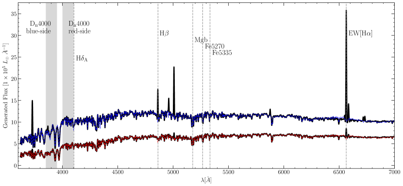
Figure 1: Example synthetic spectra constructed using the Flexible Stellar Population Synthesis models of Conroy et al. (see Section 2.2), shown by the thick black solid lines, both with a SFH of $[Z,~{}t_{q},~{}\tau]~{}=~{}[1~{}Z_{\odot},~{}10.0~{}\rm{Gyr},~{}0.5~{}\rm{Gyr}]$. Overlaid are the fits to the continuum returned by the MaNGA DAP (see Section 2.3) shown by the blue dashed line for the spectra observed at $t_{\rm{obs}}=10.4~{}\rm{Gyr}$, soon after quenching has begun, and the red dashed line for the spectra observed at $t_{\rm{obs}}=13.8~{}\rm{Gyr}$, when the spectrum is quenched. We have also labelled each of the spectral features which are used as inputs for snitch (see Section 2.4) and show their central wavelength by the dashed grey lines. The grey shaded regions show the blue- and red-side continuum regions used to measure the $\rm{D}_{n}4000$ feature. See Section 2.2.

Whilst this is the SFH we have chosen to use, it is possible for a user to provide their own SFH function by adapting the expsfh function in snitch.

2.2 Synthetic spectra generation

We then employ SPS models in order to construct synthetic spectra for the SFHs defined in Section 2.1. These synthetic spectra will be measured in the same way as an observed spectrum (see Section 2.3) in order to make a direct comparison using Bayesian statistics (see Section 2.5) to determine the ‘best fit’ SFH model for a given spectral features input.

In order to derive a realistic synthetic spectrum with our defined SFHs we used the Flexible Stellar Population Synthesis (FSPS) code of Conroy et al. (2009) and Conroy & Gunn (2010), which is written in FORTRAN, in conjunction with an existing Python wrapper by Foreman-Mackey et al. (2014). The FSPS Python wrapper makes it possible to generate spectra (or magnitudes) for any arbitrary stellar population in just two lines of code.

SPS methods rely on stellar evolution calculations to simulate all stages of stellar life, stellar spectral libraries, dust models and initial mass functions (IMFs) to translate the evolution of a hypothetical number of stars of varying ages and metallicities into a predicted integrated spectrum. FSPS also integrates CLOUDY (Ferland et al., 2013) into its spectral output so that stellar emission lines can be synthesised along with the stellar continuum. Note that other sources of ionising radiation (e.g. from shocks or active galactic nuclei; AGN) are not included in the spectral emission model in snitch. However, we note that if a user’s specific science case has need for this, it would be possible to replace the spectral synthesis function (generate_spectra) in snitch with one that does, ii in order to add another source of ionising photons. With snitch in its standard form we encourage users to ensure that contaminating emission in an observed spectrum (from shocks or AGN) has been removed or accounted for before using snitch. For example, either by fitting multiple components to spectral emission lines or by using a BPT diagram (Baldwin et al., 1981) to exclude spectra dominated by AGN or shock ionisation. If these other sources of ionising radiation are not accounted for, then the measured strength of emission due to star formation in an observed spectrum will be overestimated and the results obtained with snitch will be inaccurate. This is of particular concern for users wishing to use snitch to study merging or interacting galaxies and starburst systems; Rich et al. (2014) showed that upward of $60\%$ of the total $\rm{H}\alpha$ emission flux in late-stage gas-rich merging ultraluminous and luminous infrared galaxies (U/LIRGs) is caused by radiative shocks. Similarly Rich et al. (2015) found that shocks account for up to $30\%$ of the total $\rm{H}\alpha$ emission flux in all interacting galaxies.

In snitch we set up the FSPS models to produce spectra using the Padova isochrones (Girardi et al., 2002) and MILES spectral library (Vazdekis et al., 2016) with nebular emission, emission from dust Draine & Li (2007), a Chabrier (2003) IMF and a Calzetti et al. (2000) dust attenuation curve. We also smooth the generated synthetic spectra to have the minimum velocity dispersion measurable by MaNGA, $77~{}\rm{km}~{}{s}^{-1}$ (Bundy et al., 2015). Spectra are generated for the 22 metallicities provided in the MILES models, ranging from $0.011~{}Z_{\odot}$ to $1.579~{}Z_{\odot}$ across a logarithmic age range spanning the Universe’s history. FSPS does not allow for chemical enrichment of stellar birth material with time, i.e. the stellar populations have constant metallicity. The current version of FSPS does not allow for the $\alpha$-abundances of the stellar models to be varied. An investigation into how varying the $\alpha$-abundance would affect the generated synthetic spectra is out of the scope of this work.

These spectra are generated across a logarithmically spaced 4-dimensional array in $[t_{obs},~{}Z,~{}t_{q},~{}\tau]$ in order to facilitate faster run time during inference (see Section 2.5). These are generated for $15~{}t_{obs}$, $12~{}Z$, $50~{}t_{q}$, and $50~{}\tau$ values giving a grid of 450,000 synthetic spectra.

Two example synthetic spectra generated with FSPS for solar metallicity are shown by the solid black line in Figure 1. Note that FSPS generates spectra with flux units $L_{\odot}~{}\rm{Hz}^{-1}$, but that our spectral feature measurement procedure (see Section 2.3) requires the flux in units of $\rm{\AA}^{-1}$. The spectra both have a SFH described by the parameters $[Z,~{}t_{q},~{}\tau]~{}=~{}[1~{}Z_{\odot},~{}10.0~{}\rm{Gyr},~{}0.5~{}\rm{Gyr}]$. Overlaid are the fits to the continuum returned by the MaNGA DAP (see Section 2.3) shown by the blue dashed line for the spectra observed at $t_{\rm{obs}}=10.4~{}\rm{Gyr}$, soon after quenching has begun, and the red dashed line for the spectra observed at $t_{\rm{obs}}=13.8~{}\rm{Gyr}$, when the spectrum is quenched.

The fits are shown by the red dashed line for a spectra which has already quenched with $[Z,~{}t_{q},~{}\tau]=[1~{}Z_{\odot},~{}11.5~{}\rm{Gyr},~{}0.1~{}\rm{Gyr}]$ and by the blue dashed line for a spectra which still has some residual star formation $[Z,~{}t_{q},~{}\tau]=[1~{}Z_{\odot},~{}10.0~{}\rm{Gyr},~{}1.0~{}\rm{Gyr}]$ both observed at a redshift, $z=0.1$ (i.e. $t_{obs}=12.1~{}\rm{Gyr}$).

2.3 Measuring the synthetic spectral features

This code was originally developed for a specific science case for use with MaNGA IFU data cubes. We therefore wished to measure our synthetic spectra generated using FSPS (see Section 2.2) in the same way as the MaNGA data. It is for that reason that we use the functions defined in the MaNGA Data Analysis Pipeline (DAP; Westfall et al. in prep. and Belfiore et al. in prep.) version $2.0.2$ in order to measure the features in our synthetic spectra. If the user has a predefined method for measuring emission and absorption features in their spectra, the measure_spec function in snitch can simply be adapted.

Here we lay out the MaNGA DAP functions used in snitch to fit our synthetic spectra and obtain emission and absorption feature measurements for those unfamiliar:

1. pPXF (Cappellari & Emsellem, 2004) is used to extract a fit to the stellar continuum of a full synthetic spectrum. Here we use the version of pPXF coded into the MaNGA DAP using the PPXFFit object and the MILES template spectral libraries. To do this we assume a ‘measurement’ error on the synthetic spectra of $10\%$ of the generated flux value.

2. Using the fit to the stellar continuum provided by pPXF, we measure the emission line features in a spectrum using the Elric object and the "ELPFULL" emission line database of all 26 lines provided in the MaNGA DAP. This procedure provides emission line fluxes, equivalent widths, and kinematics from single component Gaussian fits. All strong lines are fit, as well as the Balmer series up to $\rm{H}\epsilon$ and other weaker lines.

3. We then measure the absorption indices in the emission line subtracted synthetic spectrum using the SpectralIndices object and the "EXTINDX" index database of all 42 indices provided in the MaNGA DAP. Spectral-index measurements including the $4000\rm{\AA}$ break, $\rm{TiO}$ bandhead features and the full Lick system. All indices are measured at the MaNGA resolution (specified for each index) and corrections are provided to a nominal, $\sigma_{v}=0$ measurement. The measurements of the Lick indices are provided by convolving the MaNGA data to the Lick resolution.

When we use snitch we also apply the procedure outlined above to our observed spectra to obtain synthetic and measured spectral features with the same method. We encourage users to the same where possible, either by measuring their observed spectra using the MaNGA DAP functions coded into the measure_spec function in snitch or by adapting this function to use a procedure defined by the user. It is imperative that the same spectral fitting procedure is applied to both the synthetic and observed spectra to negate the issue of model dependent emission line flux subtraction when measuring the absorption features. We note again that users should ensure that contaminating emission (e.g. from gas ionised by radiative shocks or AGN) in their observed spectrum has been removed or accounted for before using snitch (see Section 2.2).

2.4 Choosing which spectral features to use

Whilst there are many star formation sensitive spectral features used previously in the literature (see comprehensive review by Kennicutt & Evans, 2012) here we adopted a “first principles” approach. We observed how each of the 26 emission and 42 absorption features measured by the MaNGA DAP (see Section 2.3), changed across the model parameter space $[Z,t_{q},\log\tau]$ with time of observation to determine which spectral features were most sensitive to SFR, metallicity and time of observation.

We looked at how plots similar to those shown in Figure 2 for all 26 emission features and 42 absorption features changed for at different ages and metallicities. This was not a blind selection, as parameters were labelled during this study, but all features were considered across the SFH model parameter space. Many features were degenerate with other stronger spectral features or did not show strong enough variation with a change in metallicity, age or quenching parameters, ruling them out as useful features for inference. We therefore selected the following features with which to infer the SFH parameters:

1. [(i)]

2. The equivalent width (EW) of the $\rm{H}\alpha$ emission line, $\rm{EW}[\rm{H}\alpha]$, as it is the most sensitive to changes in the current SFR;

3. $\rm{H}\beta$ absorption index, as it is most sensitive to any recent, rapid quenching that has occurred;

4. $\rm{H}\delta_{A}$ absorption index, as it is the most sensitive to A-stars and therefore star formation that has been cut off within the last $\sim 1~{}\rm{Gyr}$;

5. $\rm{D}_{n}4000$ as it is most sensitive to older stars and therefore the age of the stellar population, however there is also an age-metallicity degeneracy for this feature so we also employ;

6. $\rm{[MgFe]}^{\prime}$ as it is most sensitive to the metallicity of the stellar population.

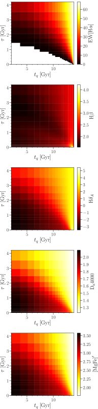
Figure 2: The variation of model spectral features across the logarithmically binned two dimensional $[t_{q},\log\tau]$ parameter space measured at $t_{obs}=13.8~{}\rm{Gyr}$ and solar metallicity, $Z=Z_{\odot}$. The features shown from top to bottom are the equivalent width of the $\rm{H}\alpha$ emission line and the spectral absorption indices $\rm{H}\beta$, $\rm{H}\delta_{A}$, $\rm{D}_{n}4000$ and $[\rm{MgFe}]^{\prime}$. Note that when a model has minimal star formation, the fitting code cannot measure an equivalent width of $\rm{H}\alpha$ therefore these values are masked out in the bottom left corner of the top panel. This figure shows how each feature is sensitive to the changing SFH and how they can be used to break the degeneracies that plague photometric studies of SFH. See Section 2.4.

Combining the spectral features listed above allows for all the different star formation timescales to be probed by using indicators of stellar populations of different ages. Of all the features listed above only $\rm{EW}[\rm{H}\alpha]$ and $\rm{D}_{n}4000$ are sensitive to the presence of dust (see Balogh et al. 1999) Unlike the $\rm{H}\alpha$ flux, which is sensitive to the current SFR, the EW[$\rm{H}\alpha$] measures the relative contribution of the $\rm{H}\alpha$ emission to the underlying continuum. Since the continuum is a proxy for stellar mass and the $\rm{H}\alpha$ emission arises around short-lived O and B stars, the EW[$\rm{H}\alpha$] is ideal for probing recent changes to the SFR in the past couple of $100$ Myr or so, in relation to the total integrated star formation over the galaxy’s lifetime (see also Li et al., 2015; Zick et al., 2018). It is worth noting that although these features were selected using this “first principles” approach, they unsurprisingly appear frequently in many works studying galaxy SFRs and histories, e.g. Kauffmann et al. (2003); Brinchmann et al. (2004); Goto (2005); Moustakas et al. (2006); Martin et al. (2007); Huang et al. (2013); Li et al. (2015); Wang et al. (2018); Spindler et al. (2018); Zick et al. (2018) to name but a few.

The variation in these five spectral features across the two dimensional $[t_{q},\log\tau]$ SFH parameter space measured at $t_{obs}=13.8~{}\rm{Gyr}$ and solar metallicity, $Z=Z_{\odot}$ is shown in Figure 2.

We note again here that only measurements from spectra dominated by emission due to gas ionisation from star formation should be input into snitch (see Section  2.2). If a user has a spectra which they think may be contaminated, we recommend modelling for or removing this contamination before measuring the emission equivalent widths. If this is not possible, e.g. due to spectral resolution constraints, then we recommend omitting the $\rm{EW}[\rm{H}\alpha]$ measurement from the list of inputs to snitch (see below and Section 4.3).

Fewer than five spectral features can be provided to snitch, although not providing one of the five does restrict the accuracy to which a SFH can be inferred (see Section 4.3). An estimate of the error on these measured values is also needed for snitch to run. The more precise the measurement of the spectral feature, the more precise the inferred SFH. It is possible for a user to adapt snitch to take any number of different spectral features which are appropriate for their scientific purpose.

2.5 Bayesian inference of SFH parameters

For the SFH problem at hand, using a Bayesian approach requires consideration of all possible combinations of the model parameters $\theta\equiv[Z,t_{q},\log\tau]$ (the hypothesis in this instance). Assuming that all galaxies formed at $t=0~{}\rm{Gyr}$, we can assume that the ‘age’ of a spectrum is equivalent to an observed time, $t_{obs}$. We used this ‘age’ to calculate the five predicted spectral features, $s,p$, at this cosmic time for a given combination of $\theta$, $\vec{d}_{s,p}(\theta,t_{obs})={s_{p}(\theta,t_{obs})}$. The predicted spectral features can now directly be compared with the five input observed spectral features $\vec{d}_{s,o}=\{s_{o}\}$ which have an associated measurement error $\vec{\sigma}_{s,o}=\{\sigma_{s,o}\}$. For a single spectrum, the likelihood of a given model $P(\vec{d}_{s,o}|\theta,t_{obs})$ can be written as:

$$P(\vec{d}_{s,o}|\theta,t_{obs})=\prod_{s=1}^{S}P(s_{o}|\theta,t_{obs})=\\ \prod_{s=1}^{S}\frac{1}{\sqrt{2\pi\sigma_{s,o}^{2}}}\exp{\left[-\frac{(s_{o}-s_{p}(\theta,t_{obs}))^{2}}{\sigma_{s,o}^{2}}\right]},$$ (2)

where $S$ is the total number of spectral features used in the inference. Here we have assumed that $P(s_{o}|\theta,t_{obs})$ are all independent of each other and that the errors on the observed features, $\sigma_{s,o}$, are also independent and Gaussian (a simplifying assumption but difficult to otherwise constrain). To obtain the probability of a set of $\theta$ values, i.e. a SFH model, given the observed spectral features: $P(\theta|\vec{d}_{s,o},t_{obs})$, we use Bayes’ theorem:

$$P(\theta|\vec{d}_{s,o},t_{obs})=\frac{P(\vec{d}_{s,o}|\theta,t_{obs})P(\theta)}{\int P(\vec{d}_{s,o}|\theta,t_{obs})P(\theta)d\theta}.$$ (3)

We assume the following prior on the model parameters so that the probability drops off at the edges of the parameter space: ${P(\theta)~{}=~{}1}$ if 0 $<Z[Z_{\odot}]\leq 1.5\text{ and }0<t_{q}~{}\rm{[Gyr]}~{}\leq 13.8~{}\text{ and }~{}0<\tau~{}\rm{[Gyr]}~{}\leq 5.9$ and ${P(\theta)~{}=~{}2\times\exp\left(\log_{10}[5.9]\right)~{}-~{}\exp\left(\log_{10}[\tau]\right)}$ otherwise.

As the denominator of Equation 3 is a normalisation factor, comparison between posterior probabilities for two different SFH models (i.e., two different combinations of $\theta=[Z,t_{q},\log\tau]$) is equivalent to a comparison of the numerators of Equation 3. Markov Chain Monte Carlo (MCMC; Mackay 2003; Foreman-Mackey et al. 2013; Goodman & Weare 2010) analysis provides us with a robust method to compare the posterior probabilities for different $\theta$ values.

MCMC allows for an efficient exploration of the parameter space by avoiding areas with low likelihood. A large number of ‘walkers’ are started at an initial position (i.e. an initial guess at the SFH, $\theta$) from which they each individually ‘jump’ a randomised distance to a new position. If the probability in this new position is greater than the calculated probability at the original position then a ‘walker’ accepts this change. Any new position then influences the direction of the ‘jumps’ of other walkers (true for ensemble MCMC only). This is repeated for a specified number of jumps after an initial ‘burn-in’ phase. The length of this burn-in phase is determined after sufficient experimentation to ensure that the ‘walkers’ have converged on the global minimum within the defined number of steps. Here we use emcee, (Foreman-Mackey et al., 2013), an affine invariant ensemble sampler written in Python to explore the SFH parameter space for a given set of measured spectral features. emcee returns the positions of the ‘walkers’ in the predefined parameter space, which are analogous to the regions of high posterior probability, $P(\theta|\vec{d}_{s,o},t_{obs})$.

For each run of snitch, the inference run is initialised with 100 walkers with a burn-in phase of 1000 steps before a main run of 200 steps. Acceptance fractions for each walker are difficult to estimate due to the fact that walkers often get stuck in local minima during a run (see Section 2.6 for more information).

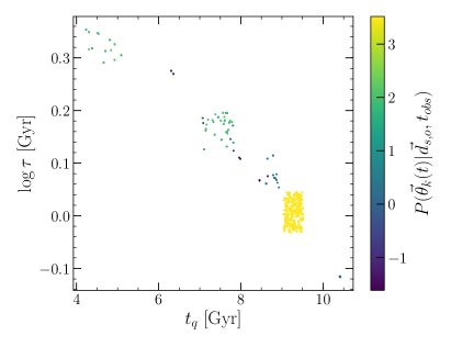
Figure 3: This figure shows the walker positions marginalized over the $Z$ dimension into the two dimensional $[t_{q},\log\tau]$ space and coloured by their characteristic $P(\vec{\theta}_{k}(t)|\vec{d}_{s,o},t_{obs})$ value (see Equation 3). The higher the value of their log probability, the more likely the model is. The lower values of log probability for some groups of walkers suggests that these are indeed stuck in local minima. These clusters of walkers in local minima can be ‘pruned’ (see Section 2.6) away to leave only the global minimum in the final output. Note that since we employ a nearest neighbours interpolation method across the look-up table (see Section 2.5) the resulting global minimum in parameter space traces the grid structure of the look-up table. See Section 2.6.

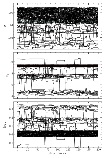
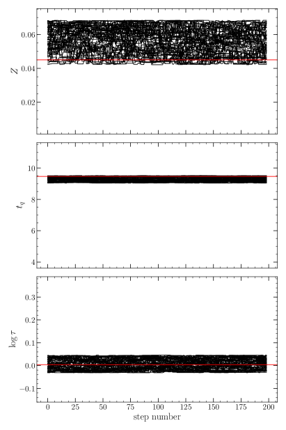
Figure 4: The positions traced by the emcee walkers with step number (i.e. time) in each of the $[Z,t_{q},\log\tau]$ dimensions in the post burn-in phase before pruning (left) and after pruning (right). Walkers have got stuck in local minima (see also Figure 3) but some have managed to find the global minimum. The right panel therefore shows how the walkers left after pruning have fully explored the global minimum around the known true values (shown by the red lines in each panel). See Section 3.

With each ‘walker’ jump to a new place in parameter space, a synthetic spectra must be generated then measured, as described in Section 2.3, to produce predicted spectral parameters. Since this is very computationally expensive, a 4-dimensional look-up table of each of the five spectral parameters listed in Section 2.4 was generated across a logarithmically spaced grid in $[t_{obs},~{}Z,~{}t_{q},~{}\tau]$. We initialised our look-up table over a non-regular grid in order to optimise the number of useful $t_{q}$ values for each $t_{obs}$ value, i.e. quenched SFHs with $t_{q}\leq t_{obs}$. Those SFHs with $t_{q}>t_{obs}$ had constant SFR and so returned the same values for the spectral parameters regardless of the $t_{q},\log\tau$ values. This allowed us to construct a finer array in $t_{q}$ for each value of $t_{obs}$ to pinpoint recent changes in the SFH more precisely. Figure 2 shows a slice in two dimensions of this look-up table, for $t_{obs}=13.8~{}\rm{Gyr}$ and solar metallicity, $Z=Z_{\odot}$ for each of the five spectral parameters.

The look-up table is interpolated over (using a nearest neighbour approach to speed up run time over the irregular grid) to find spectral parameters for each ‘walker’ jump to any new position in $[t_{obs},~{}Z,~{}t_{q},~{}\log\tau]$ parameter space.

2.6 Pruning walkers stuck in local minima

After running snitch and inspecting the walker positions it became apparent that the walkers of emcee would often get stuck in local minima. We therefore implemented a pruning method, as described in Hou et al. (2012), in order to remove those walkers in local minima leaving only the global minima from which to derive inferred SFH parameters. The method outlined in Hou et al. (2012) is a simple one dimensional clustering method wherein the average negative log-likelihood for each walker is collected. This results in $L$ numbers; $\overline{l}_{k}$:

$$\overline{l}_{k}=\frac{1}{T}\sum^{T}_{t=1}P(\vec{\theta}_{k}(t)|\vec{d}_{s,o},t_{obs}),$$ (4)

where T is the total number of steps each walker, $k$, takes. $\vec{\theta}_{k}(t)$ is therefore the set of walker positions at a given step, $t$ in the MCMC chain. These $L$ numbers, $\overline{l}_{k}$, are therefore characteristic of the well which walker $k$ is in, so that walkers in the same well will have similar $\overline{l}_{k}$ (see Figure 3 in which walkers are coloured by their characteristic $P(\vec{\theta}_{k}(t)|\vec{d}_{s,o},t_{obs})$ value).

The walkers are all then ranked in order of decreasing average log likelihood, $\overline{l}_{(k)}$, or increasing $-\log\overline{l}_{(k)}$. If there are big jumps in the $-\log\overline{l}_{(k)}$, these are easy to spot and are indicative of areas where walkers have got stuck in local minima. The difference in $-\log\overline{l}_{(k)}$ for every adjacent pair of walkers is calculated. The first pair whose difference is a certain amount larger than the average difference previously is then identified like so:

$$-\log\overline{l}_{(j+1)}+\log\overline{l}_{(j)}>Const−\frac{\log\overline{l}_{(j)}+log\overline{l}_{(1)}}{j-1}.$$ (5)

After some trial and error we decided on a constant value of $Const=10000$. All the walkers with with $k>j$ are thrown away and only the ones with $k\leq j$ are kept after being identified as part of the global minimum. This can be seen in Figure 4 wherein the walker positions at each step before pruning are shown in comparison to those after pruning in the main run stage. In the cases where the ‘walkers’ did not get stuck in local minima, this pruning routine leaves the walker chains untouched.

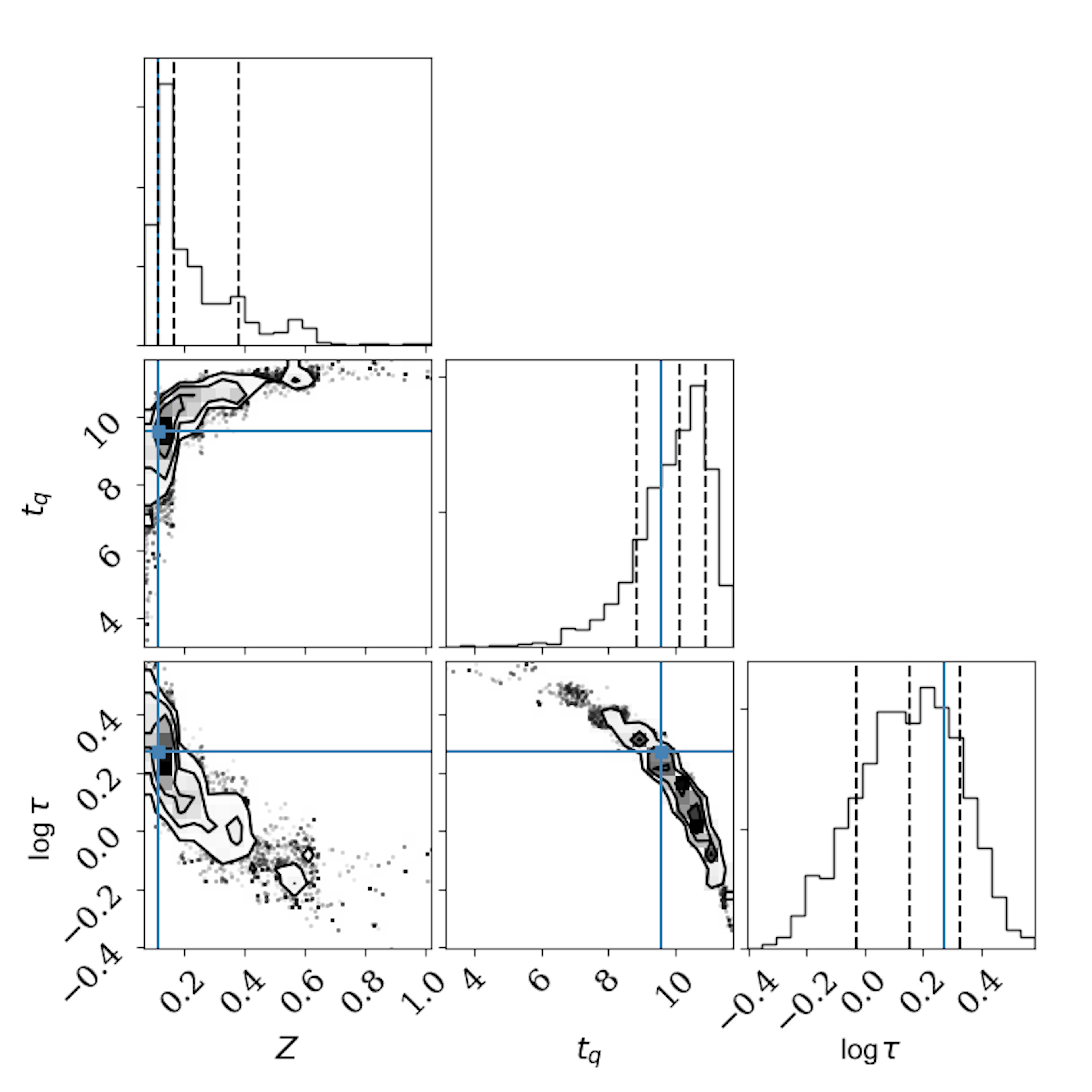
Figure 5: Example output from snitch showing the posterior probability function traced by the MCMC walkers across the three dimensional parameter space $[Z,t_{q},\log\tau]$. Dashed lines show the 18th, 50th and 64th percentile of each distribution function which can be interpreted as the ‘best fit’ with $\textpm 1\sigma$. The blue lines show the known true values which snitch has managed to recover. See Section 3.

3 Output of Code

The burn-in and main run walker positions and posterior probabilities at each step are saved by snitch. From this three dimensional MCMC chain charting the $[Z,t_{q},\log\tau]$ positions of the walkers around parameter space, the ‘best fit’ $[Z,t_{q},\log\tau]$ values along with their uncertainties can be determined from the 16th, 50th and 84th percentile values of the walker positions. These values are quoted by snitch at the end of a run. An example output from snitch for the predicted spectral features of a single known model SFH with a synthetic spectrum constructed with the FSPS models (see Section 2.2) is shown in Figure 5. This figure is also saved by snitch upon completion of a run.

The required inputs for snitch to run on a single spectrum are at least one, if not all, of $\rm{EW}[\rm{H}\alpha]$, $\rm{D}_{n}4000$, $\rm{H}\beta$, $\rm{H}\delta_{A}$ and $\rm{[MgFe]}^{\prime}$ and their associated errors and the galaxy redshift, $z$. To run snitch on a typical laptop on the spectral features of a single spectrum takes approximately 2 minutes.

4 Testing

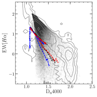
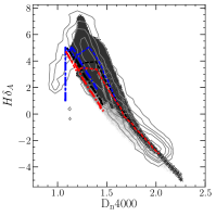
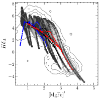
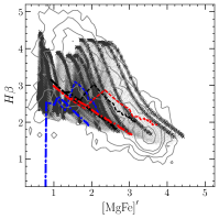
Figure 6: Consistency test between actual spectral parameter measurements of the central spaxels (with $R/R_{e}<0.1$) of all MPL-6 MaNGA galaxies (grey contours) and those measured from the synthetic spectra generated for the look-up table (transparent black crosses; see Section 2.5). The contours enclose $(11,39,68,86,96)\%$ of the spaxel measurements in each panel. We also show the tracks across cosmic time for a synthetic spectrum with constant SFR (thick dot-dashed lines) and for a synthetic spectrum with model quenching parameters $[\rm{t}_{q},\tau]=[10.0,0.5]~{}\rm{Gyr}$ (thin dashed lines; a relatively rapid quench) for $0.2~{}\rm{Z}_{\odot}$, $1.0~{}\rm{Z}_{\odot}$ and $1.6~{}\rm{Z}_{\odot}$ metallicities in blue, black and red respectively. We have not attempted to recreate the distributions across spectral parameter space seen for this sample of real galaxy spectra (see Section 4.4 and Figure 7 for such a test), we are merely showing the spectral parameters for the set of quenching SFHs we have generated across the 4-dimensional look-up table (in which $t_{obs}>11.85~{}\rm{Gyr}$, i.e. $z\mathrel{\hbox{\hbox to0.0pt{\hbox{\lower 3.0pt\hbox{$\sim$}}\hss}\hbox{\raise 2.0pt\hbox{$<$}}}}0.15$, rather than covering all of cosmic time like the tracks shown by the dashed and dot-dashed lines), which we have shown in Figure 2 are degenerate. See Section 4.1.

4.1 Consistency of spectral parameter measurements

Before testing the performance of the code, we tested the consistency of the measurements of the predicted spectral parameters generated in the look-up table (see Section 2.5 and Figure 2). To do this, we collated the spectral parameters for all the central spaxels (with $R/R_{e}<0.1$ to give a reasonable sample size) of all MPL-6 MaNGA galaxies using the Marvin interface developed for MaNGA (Cherinka et al., 2018). These are shown by the black contours in each of the panels of Figure 6. Overlaid are points showing the spectral measurements for the synthetic FSPS spectra from the look-up table. We can see that similar ranges are found for the modelled SFHs as for the spaxels of real MaNGA galaxies, suggesting that the models produced are appropriately generated and measured. Note that we have not attempted to recreate the distributions across spectral parameter space seen for this sample of real MaNGA galaxy spectra (see Section 4.4 for such a test). We are merely showing the spectral parameters for the set of quenching SFHs we have generated across the 4-dimensional look-up table (in particular where $t_{obs}>11.85~{}\rm{Gyr}$, i.e. $z\mathrel{\hbox{\hbox to0.0pt{\hbox{\lower 3.0pt\hbox{$\sim$}}\hss}\hbox{\raise 2.0pt\hbox{$<$}}}}0.15$ rather than covering all of cosmic time). Therefore we do not expect to cover the full range in spectral parameters seen for the real MaNGA galaxy spectra, since these will also include spectra that are starbursting, have increasing star formation rates or contain younger stellar populations. Whereas snitch is specifically designed to target the properties of quenching stellar populations.

4.2 Testing precision

In order to test that snitch can find the correct quenched SFH model for a given set of spectral features, 25 synthesised galaxy spectra were created with known SFH parameters (i.e. known randomised values of $\theta=[Z,t_{q},\log\tau]$) from which synthetic spectra were generated and predicted spectral features were measured (see Section 2.2). These were input into snitch, assuming a $10\%$ error on each spectral parameter measurement, to test whether the known values of $\theta$ were reproduced, within error, for each of the 25 synthesised galaxies. In all cases the true values reside within the parameter space explored by the walkers left over after pruning, which trace the global minimum of the posterior probability. snitch therefore succeeds in locating the true parameter values within the degeneracies of the SFH model for known values. However, the spread in the walker positions generally gets broader as the inferred $\tau$ value gets larger (i.e. longer quench) and the inferred $t_{q}$ value gets smaller (i.e. earlier quench). This is a product of both the logarithmic spacing in the look-up table generated for use in snitch (see Section 2.5) and an observational effect, since spectral signatures of a longer, earlier quench will have been washed out over time.

This test demonstrates how snitch is precise in recovering the parameters describing the true SFHs, however that precision varies across the parameter space. The median difference between known and inferred parameter values for 25 random SFHs is $[\Delta Z,~{}\Delta t_{q},~{}\Delta\tau]~{}=~{}[0.1~{}\rm{Z}_{\odot},~{}0.3~{}\rm{Gyr},~{}0.2~{}\rm{Gyr}]$ and the maximum difference between the inferred and true values are $[\Delta Z,~{}\Delta t_{q},~{}\Delta\tau]~{}=~{}[0.7~{}\rm{Z}_{\odot},~{}3.7~{}\rm{Gyr},~{}1.4~{}\rm{Gyr}]$.

Table 1: The mean uncertainties ($\pm 1\textpm\sigma$) on the best fit and difference in known and best fit values ($\Delta[Z,t_{q},\tau]$) for the 10 synthesised galaxy spectra returned when each spectral feature is omitted in turn. The accuracy in determining the metallicity, $Z$, parameter is most affected by the removal of $\rm{[MgFe]}^{\prime}$ and $\rm{D}_{\rm{n}}4000$. The accuracy in determining the time of quenching, $t_{q}$, parameter is most affected by the removal of $\rm{H}\beta$, $\rm{H}\delta_{A}$ and $\rm{D}_{\rm{n}}4000$. The accuracy in determining the rate of quenching, $\tau$, parameter is most affected by the removal of $\rm{H}\delta_{A}$, $\rm{EW}[\rm{H}\alpha]$ and $\rm{D}_{\rm{n}}4000$. See Section 4.3.

Spectral feature omitted	None	$\rm{H}\alpha$	$\rm{D}_{\rm{n}}4000$	$\rm{H}\beta$	$\rm{H}\delta_{A}$	$\rm{[MgFe]}^{\prime}$
Average uncertainty, Z $1\sigma$	$0.2$	$0.3$	$0.2$	$0.2$	$0.2$	$0.4$
Average uncertainty, $t_{q}$ $1\sigma~{}$	$1.1$	$1.9$	$1.7$	$2.1$	$3.2$	$2.4$
Average uncertainty, $\tau$ $1\sigma~{}$	$0.4$	$0.8$	$0.9$	$0.5$	$0.5$	$0.8$
$\Delta Z~{}\rm{[Gyr]}~{}$	$0.1$	$0.1$	$0.3$	$0.2$	$0.1$	$0.3$
$\Delta t_{q}~{}\rm{[Gyr]}~{}$	$0.3$	$1.3$	$1.6$	$1.5$	$1.9$	$0.8$
$\Delta\tau~{}\rm{[Gyr]}~{}$	$0.2$	$2.3$	$1.4$	$2.1$	$2.6$	$1.5$

4.3 Testing precision when less spectral information provided

snitch is designed so that not all of the spectral features have to be provided for the code to return an inferred quenching history. This is a particularly useful feature if the user is unable to obtain or measure a certain spectral feature. For example, if measurements are being obtained from archival data or a feature lies outside of the wavelength range of their spectrum.

Users should note that quenching histories inferred given fewer inputs results in a larger uncertainty on the quoted best fit parameters returned by snitch. To quantify this we generated 10 random $[Z,t_{q},\log\tau]$ values and used them to generate synthetic spectra, in which the predicted spectral features were measured and used as inputs to snitch, each time omitting one of the spectral features from the list of inputs. The mean uncertainties on the best fit and difference between known and best fit values returned when each spectral feature is omitted are quoted in Table 1. The accuracy in determining the metallicity, $Z$, parameter is most affected by the removal of $\rm{[MgFe]}^{\prime}$ and $\rm{D}_{\rm{n}}4000$. The accuracy in determining the time of quenching, $t_{q}$, parameter is most affected by the removal of $\rm{H}\beta$, $\rm{H}\delta_{A}$ and $\rm{D}_{\rm{n}}4000$. The accuracy in determining the rate of quenching, $\tau$, parameter is most affected by the removal of $\rm{H}\delta_{A}$, $\rm{EW[H}\alpha]$ and $\rm{D}_{\rm{n}}4000$.

For further combinations of missing parameters, we suggest the user completes their own tests to determine how the quoted uncertainty will change with the omission of more than one spectral feature. However, we do not recommend using snitch if the number of available spectral features is less than $4$. If this is the case, the number of inputs given to the code will be equal to or less than the number of parameters to be inferred and the resulting SFH will be unreliable.

4.4 Population testing

Figure 7: The distribution, from right to left of the $\log_{10}$EW$[\rm{H}\alpha]$, $\rm{H}\beta$, $\rm{[MgFe]}^{\prime}$, $\rm{H}\delta_{A}$ and $\rm{D}_{\rm{n}}4000$ values of a random spaxel in each of $150$ randomly selected observed MaNGA galaxies (black solid line). In each panel the distribution of the snitch inferred spectral parameter is shown by the red dashed line. See Section 4.5

A further test of snitch is to determine whether the inferred SFH parameters, $[Z,~{}t_{q},~{}\log\tau]$, can reproduce the distribution of observed spectral features of a sample of galaxy spectra. We randomly selected a spaxel from each of $150$ MaNGA MPL-6 galaxies and used the observed spectral parameters as inputs to snitch. We then used the inferred SFH parameters returned by snitch to estimate inferred spectral parameters for each of the $150$ galaxy spaxels. In order to add noise to these inferred spectral parameters, we also added a random multiple of the error on the observed spectral features, drawn from a Gaussian distribution with mean of $0$ and standard deviation of $1.1$ (i.e. normally distributed between roughly $-3$ and $3$ so that the noise added to the inferred value is distributed between $\pm 3\sigma$).

Figure 7 shows the distributions of the inferred and measured spectral parameters and highlights how the inferred values trace the original measured values well, in particular for the absorption features. Once again demonstrating that snitch can return a precise SFH for a galaxy spectrum.

However, we can see that snitch appears to struggle to reproduce the distribution of $\log_{10}$EW$[\rm{H}\alpha]$. This is due to the fact that the look-up tables which snitch uses are masked for $\log_{10}$EW$[\rm{H}\alpha]~{}\mathrel{\hbox{\hbox to0.0pt{\hbox{\lower 3.0pt\hbox{$\sim$}}\hss}\hbox{\raise 2.0pt\hbox{$<$}}}}~{}1$ (see left most panel of Figure 2) as these values become unreliable measurements due to the contamination from the nearby $[NII]$ doublet. Therefore the inferred SFH found by snitch will have a null EW$[\rm{H}\alpha]$ value where star formation is minimal. This was true for $92$ of the $150$ galaxy spaxels and so these values are not plotted in the distribution shown by the red curve in the left most panel of Figure 7. We did not mask the observed EW$[\rm{H}\alpha]$ values in order to provide snitch with five inputs for each MaNGA galaxy, as a control, so these values are still shown in the distribution shown by the black curve in the left most panel of Figure 7.

4.5 Testing accuracy

We have shown in the previous section that snitch can return precise known values for SFHs, however now we must test its accuracy. In order to quantify this we have run snitch on spectra which have previously derived SFHs. Firstly, on those which have had similar simple models derived (Section 4.5.1) and then on spectra with SFHs from hydrodynamic simulations (Section 4.5.2).

Table 2: The mean star formation fraction (SFF) in each age bin for the six galaxy samples quoted by (Tojeiro et al., 2013, TSFF) and returned by snitch. Each value is quoted with an uncertainty, for the Tojeiro et al. (2013) values this is quoted as the standard error on the mean for each bin with the same precision as Tojeiro et al. quote in their Table 2. For the snitch values the uncertainty stated is calculated from the SFH parameters at the $16$th and $84$th walker positions (see Section 2.5) and are quoted to a the nearest whole number since the snitch uncertainties are much broader than the ones calculated by Tojeiro et al. The SFF and $1\sigma$ errors are given in units of $10^{-3}$. See Section 4.5.1.

Look-back time	$0.01-0.074~{}\rm{Gyr}$		$0.074-0.425~{}\rm{Gyr}$		$0.425-2.44~{}\rm{Gyr}$		$2.44-13.7~{}\rm{Gyr}$
	TSFF	snitch SFF	TSFF	snitch SFF	TSFF	snitch SFF	TSFF	snitch SFF
Red ellipticals	$0.11\pm 0.047$	$1\pm_{1}^{1}$	$0.32\pm 0.052$	$1\pm_{1}^{1}$	$33\pm 1$	$2\pm_{2}^{13}$	$966\pm 2.89$	$996\pm_{6}^{1}$
Red ET spirals	$0.65\pm 0.45$	$10\pm_{9}^{19}$	$2.4\pm 0.023$	$22\pm_{21}^{44}$	$36\pm 3.8$	$244\pm_{241}^{488}$	$960\pm 8.4$	$997\pm_{276}^{1}$
Red LT spirals	$1.9\pm 1.18$	$61\pm_{59}^{121}$	$5.6\pm 0.0097$	$113\pm_{111}^{225}$	$59\pm 12$	$315\pm_{311}^{630}$	$933\pm 18.7$	$997\pm_{501}^{1}$
Blue ellipticals	$2.5\pm 1.3$	$108\pm_{107}^{217}$	$11\pm 0.3$	$186\pm_{184}^{372}$	$52\pm 11$	$319\pm_{315}^{637}$	$934\pm 17.2$	$997\pm_{638}^{1}$
Blue ET spirals	$4.9\pm 1.1$	$80\pm_{79}^{46}$	$14\pm 0.14$	$134\pm_{133}^{74}$	$42\pm 5.2$	$211\pm_{209}^{86}$	$938\pm 9.2$	$554\pm_{217}^{437}$
Blue LT spirals	$6.1\pm 1.4$	$67\pm_{66}^{58}$	$11\pm 0.34$	$113\pm_{109}^{94}$	$43\pm 12$	$187\pm_{184}^{113}$	$939\pm 19.3$	$615\pm_{279}^{372}$

4.5.1 Comparing with other SFH inference codes

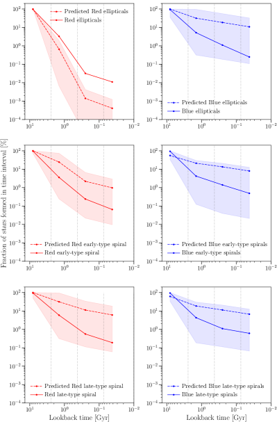
Figure 8: The mean star formation fraction (SFF) in each age bin for the six galaxy samples analysed by (Tojeiro et al., 2013, solid lines) and returned by snitch (dashed lines). We have reproduced these plots in the exact same way as presented in Figure 7 of Tojeiro et al. except that we have flipped the x-axis so that more recent epochs are on the right hand side for continuity with the rest of the figures in this work. The shaded region shows the $1\sigma$ error on the predicted SFF inferred by snitch. Note the logarithmic y-axis scale, given the large uncertainty in predicted SFFs inferred by snitch. These results suggest that SNITCH does return an accurate parametrised model of SFH, however when snitch is less accurate in its inference of the SFH this is reflected in the large uncertainties returned. See Section 4.5.1.

In the case of the previously fitted simple SFH models, we have compared the results of snitch with the parametrised SFHs derived by Tojeiro et al. (2013) for $6$ stacked SDSS spectra of $13959$ red ellipticals, $381$ blue ellipticals, $5139$ blue late-type (LT) spirals, $294$ red LT spirals, $1144$ blue early-type (ET) spirals and $1265$ red ET spirals. We measured the spectral features of each of the $6$ stacked spectra using the method outlined in Section 2.3 and input them into snitch. Since Tojeiro et al. quoted their results in terms of the fraction of stars formed (SFF) in a given time period, we have followed the same method. In Table 2 we have listed the SFF for the six samples found by Tojeiro et al. and the SFF for the best fit parameters inferred by snitch along with the uncertainty. These results are also plotted in Figure 8, recreating Figure 7 of Tojeiro et al.

We can see from these results that snitch broadly agrees with the results of Tojeiro et al., within the uncertainties. However, the uncertainties returned by snitch are much broader for blue galaxies, particular for ET spirals, as seen in Figure 8. This is to be expected since snitch fits a quenching SFH model to a galaxy spectrum and so would return a less accurate SFH for star forming spectra (see Section 4.6.1). There is also some discrepancy between the recent SFFs inferred by snitch and quoted by Tojeiro et al. for the red ellipticals. This is presumably because of the incredibly small SFFs occurring at these recent epochs, which are difficult to constrain. Quenching must therefore have occurred at early epochs in these red ellipticals, which will dilute the spectral features giving rise to an uncertain fit. These results suggest that snitch does return an accurate parametrised model of SFH at least for galaxies which are currently quenching or recently fully quenched (within at least the last $\sim 2.5~{}\rm{Gyr}$, i.e. $z\mathrel{\hbox{\hbox to0.0pt{\hbox{\lower 3.0pt\hbox{$\sim$}}\hss}\hbox{\raise 2.0pt\hbox{$<$}}}}0.2$), however when snitch is less accurate in its inference of the SFH this is reflected in the large uncertainties returned.

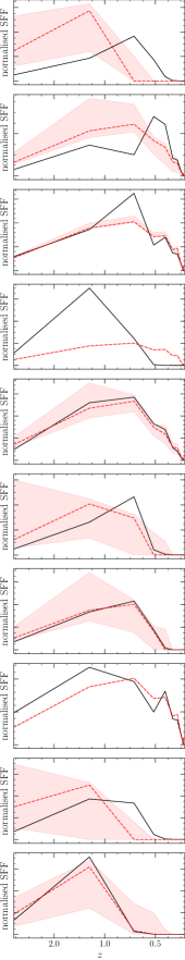
Figure 9: Comparison of the SFFs generated by Lgalaxies (black) and those inferred by snitch (red, dashed with shaded uncertainty regions; note that two panels have very small uncertainties) for $10$ randomly selected synthetic spectra with SFRs in the range $0~{}<~{}\rm{SFR}~{}[M_{\odot}~{}\rm{yr}^{-1}]~{}<~{}1$, and stellar masses $10^{9}~{}<~{}M_{*}~{}[M_{\odot}]~{}<~{}10^{11}$. Note how snitch is sensitive to the most recent change in the SFF. See Section 4.5.2.

Figure 10: Comparison of the difference between the calculated and inferred time of maximum SFR ($\Delta\log t_{\rm{max}}$; left) and time for the SFR to drop to half of the maximum value ($\Delta\log t_{1/2}$; right) for the $104$ synthetic SFHs with a non zero quasar accretion rate generated by LGalaxies. See Section 4.5.2.

4.5.2 Comparing with known SFHs from hydrodynamic simulations

We generated $8238$ simulated galaxy SFHs using the LGalaxies suite of hydrodynamic simulations (Henriques et al., 2015) at a redshift of $z=0.043$ (the mean redshift of the MaNGA DR14 sample) with a range of SFRs, $0<\rm{SFR}~{}[M_{\odot}~{}\rm{yr}^{-1}]<1$, and stellar masses $10^{9}<M_{*}[M_{\odot}]<10^{11}$. Of these $8238$ simulated galaxies we selected all of those flagged by LGalaxies to have a quasar accretion rate above zero. This resulted in $104$ simulated galaxy SFHs. We used the FSPS models of Conroy & Gunn (2010) to generate synthetic spectra for each of these $104$ simulated SFHs (as described in Section 2.2) and then measured their spectral features using the MaNGA DAP functions outlined in Section 2.3. We then input these measurements into snitch to derive the best fit $[Z,t_{q},\log\tau]$ parameters for our simple model of SFH to compare with the known SFH output by the hydrodynamic simulation. This test is therefore very similar to our tests with different known SFHs that we generated in Section 4.2, however the SFHs generated by the hydrodynamic simulation can be classed as both more varied and more characteristic of real galaxy SFHs in this case.

Figure 9 shows the normalised SFFs as generated by Lgalaxies and inferred for their spectra by snitch for $10$ randomly selected simulated SFHs. We can see that the output from snitch largely agrees, within the uncertainties, with the known SFHs of Lgalaxies. Although not all details of the Lgalaxies SFHs are reproduced, snitch identifies the most recent epoch with a dramatic change in the SFR.

We can also generalise the SFHs generated by Lgalaxies and inferred by snitch into two parameters, the time of maximum SFR, $\log t_{\rm{max}}$, and the time for the SFR to drop to half of the maximum value ($\log t_{1/2}$). Note, that if a galaxy’s SFR is increasing then we cannot derive a value for $t_{1/2}$. These generalised parameters roughly trace the exponential SFH parameters of $t_{q}$ and $\tau$, but allow for a comparison to the SFHs generated by Lgalaxies which are not constrained to an analytic form. Figure 10 shows the difference between the generated and inferred values of $\log t_{\rm{max}}$ & $\log t_{1/2}$. We can see that for the majority of synthetic spectra the inferred SFH parameters are comparable to those generated by Lgalaxies. However there is a much larger spread in $\Delta\log t_{1/2}$ (shown in the right panel of Figure  10) than in $\Delta\log t_{\rm{max}}$ (shown in the left panel), suggesting that for galaxies with more complex SFHs, snitch will return a more accurate value for the time of quenching, $t_{q}$, than for the rate that quenching occurs, $\log\tau$.

4.6 Testing performance with different SFH definitions

4.6.1 Star Forming SFHs

We must also understand how snitch behaves when spectral parameters derived from a star forming galaxy spectrum are input. Figure 11 shows the example output from snitch across the three dimensional parameter space $[Z,t_{q},\log\tau]$ for a synthetic galaxy spectrum which is still star forming at a constant rate at the time of observation, $t_{obs}$. Note that the walkers have explored only the parameter space where $t_{q}>t_{obs}$, i.e. the observed redshift of the galaxy (see Section 2.2), and all possible values of $\log\tau$, since the synthetetic galaxy has not yet quenched and therefore all quenching rates are equally likely.

Figure 11: Example output from snitch showing the posterior probability function traced by the MCMC walkers across the three dimensional parameter space $[Z,t_{q},\log\tau]$, for a synthetic galaxy spectrum which is still star forming with a constant SFR. Dashed lines show the 18th, 50th and 64th percentile of each distribution function which can be interpreted as the ‘best fit’ with $1\sigma$. The blue lines show the known true values which snitch has managed to recover, within the uncertainties. Note that the walkers have explored only the parameter space where $t_{q}>t_{obs}$, i.e. the observed redshift of the galaxy (see Section 2.2), and all possible values of $\log\tau$, since the synthetic galaxy has not yet quenched and therefore all quenching rates are equally likely. See Section 4.6.1.

4.6.2 Different Forms of Quenching SFHs

Obviously, not all galaxies will be accurately described by an exponentially quenching SFH. In special use cases (for example studying post starburst galaxies) a different SFH may be defined by the user by replacing the expsfh function with their own.

However, we have also tested how snitch behaves when spectra with known SFHs of different forms are input. We tested spectra with burst, many burst, normal and log-normal models of SFH, all of which are often used in the literature to model simple SFHs.

We found that snitch was always sensitive to the most recent epoch of star formation or quenching. For the burst and many-burst models, snitch returns a constant SFR up until the peak of the last burst at which point quenching happens very rapidly. Similarly for the log normal and normal SFHs, snitch returns a best fit SFH with constant SFR until the peak of the normal at which point it declines at a rate comparable to the drop off of the Gaussian SFH. All of these tests suggest that snitch is most sensitive to the most recent epoch of star formation but can also roughly trace the quenching of star formation even if the true decline does not occur at an exponential rate.

5 Conclusions

Given the recent influx of spectral data from integral field unit (IFU) surveys, there is need for a tool that allows a user to quickly derive a simple, informative star formation history (SFH) in order to compare the SFHs of spectra within a single IFU data cube or across a large population of galaxy spectra. We have therefore developed snitch, an open source Python package which uses a set of five absorption and emission spectral features to infer the best fit parameters describing an exponentially declining model of SFH. To do this, snitch assumes a set of SFH parameters and convolves them with a stellar population synthesis (SPS) model to generate a synthetic spectrum. The predicted absorption and emission spectral features are then measured in this synthetic spectrum (using the same method developed to fit the observed spectra in MaNGA data cubes). The predicted spectral features for many different model SFHs are then compared to the input observed spectral features by snitch to find the best fit SFH model using Bayesian statistics and an MCMC method. snitch returns the best fit time of quenching, exponential rate of quenching and SPS model metallicity to the input spectral features. The typical run time for a single spectrum is around 2 minutes on a laptop machine.

snitch was developed for specific use on the MaNGA IFU data cubes, however, it is fully customisable by the user for a specific science case, for example by changing the SFH model, spectral features used in the inference or the method used to measure spectral features in the synthetic spectra. We advocate for the use of snitch as a comparative tool within an IFU data cube or across a large population of spectra, rather than to derive a detailed SFH of a single spectra due to the generalising nature of the analytic SFH model.

We have demonstrated with rigorous testing that snitch is both precise and accurate at inferring the parameters describing an exponentially declining model of SFH. These tests suggest that snitch is sensitive to the most recent epoch of star formation but can also trace the quenching of star formation even if the true decline does not occur at an exponential rate.

References

- Abramson et al. (2016) Abramson L. E., Gladders M. D., Dressler A., Oemler A., Poggianti B., Vulcani B., 2016, ArXiv e-prints
- Baldwin et al. (1981) Baldwin J. A., Phillips M. M., Terlevich R., 1981, PASP, 93, 5
- Balogh et al. (1999) Balogh M. L., Morris S. L., Yee H. K. C., Carlberg R. G., Ellingson E., 1999, ApJ, 527, 54
- Blanton et al. (2017) Blanton M. R., Bershady M. A., Abolfathi B., Albareti F. D., Allende Prieto C., Almeida A., Alonso-García J., Anders F., Anderson S. F., Andrews B., et al. 2017, AJ, 154, 28
- Brinchmann et al. (2004) Brinchmann J., Charlot S., White S. D. M., Tremonti C., Kauffmann G., Heckman T., Brinkmann J., 2004, MNRAS, 351, 1151
- Bryant et al. (2015) Bryant J. J., Owers M. S., Robotham A. S. G., Croom S. M., Driver S. P., Drinkwater M. J., Lorente N. P. F., Cortese L., Scott N., Colless M., Schaefer A., Taylor E. N., Konstantopoulos I. S., Allen J. T., Baldry I., 2015, MNRAS, 447, 2857
- Bundy et al. (2015) Bundy K., Bershady M. A., Law D. R., Yan R., Drory N., MacDonald N., Wake D. A., Cherinka B., Sánchez-Gallego J. R., Weijmans A.-M., Thomas D., et a., 2015, ApJ, 798, 7
- Burstein et al. (1984) Burstein D., Faber S. M., Gaskell C. M., Krumm N., 1984, ApJ, 287, 586
- Burstein et al. (1986) Burstein D., Faber S. M., Gonzalez J. J., 1986, AJ, 91, 1130
- Calzetti et al. (2000) Calzetti D., Armus L., Bohlin R. C., Kinney A. L., Koornneef J., Storchi-Bergmann T., 2000, ApJ, 533, 682
- Cappellari & Emsellem (2004) Cappellari M., Emsellem E., 2004, PASP, 116, 138
- Chabrier (2003) Chabrier G., 2003, PASP, 115, 763
- Cherinka et al. (2018) Cherinka B., Sánchez-Gallego J., Andrews B., Brownstein J., , 2018, 10.5281/zenodo.1146705, sdss/marvin: Marvin Beta 2.2.0
- Chevallard & Charlot (2016) Chevallard J., Charlot S., 2016, MNRAS, 462, 1415
- Chilingarian (2009) Chilingarian I. V., 2009, MNRAS, 394, 1229
- Chilingarian & Asa’d (2018) Chilingarian I. V., Asa’d R., 2018, ApJ, 858, 63
- Chilingarian et al. (2011) Chilingarian I. V., Mieske S., Hilker M., Infante L., 2011, MNRAS, 412, 1627
- Cid Fernandes et al. (2005) Cid Fernandes R., Mateus A., Sodré L., Stasińska G., Gomes J. M., 2005, MNRAS, 358, 363
- Conroy et al. (2014) Conroy C., Graves G. J., van Dokkum P. G., 2014, ApJ, 780, 33
- Conroy & Gunn (2010) Conroy C., Gunn J. E., 2010, ApJ, 712, 833
- Conroy et al. (2009) Conroy C., Gunn J. E., White M., 2009, ApJ, 699, 486
- Draine & Li (2007) Draine B. T., Li A., 2007, ApJ, 657, 810
- Dressler (2004) Dressler A., 2004, in Diaferio A., ed., IAU Colloq. 195: Outskirts of Galaxy Clusters: Intense Life in the Suburbs Infall and starbursts in z [similar] 0.5 clusters. pp 341–346
- Faber et al. (1985) Faber S. M., Friel E. D., Burstein D., Gaskell C. M., 1985, The Astrophysical Journal Supplement Series, 57, 711
- Ferland et al. (2013) Ferland G. J., Porter R. L., van Hoof P. A. M., Williams R. J. R., Abel N. P., Lykins M. L., Shaw G., Henney W. J., Stancil P. C., 2013, Rev. Mexicana Astron. Astrofis., 49, 137
- Foreman-Mackey et al. (2013) Foreman-Mackey D., Hogg D. W., Lang D., Goodman J., 2013, PASP, 125, 306
- Foreman-Mackey et al. (2014) Foreman-Mackey D., Sick J., Johnson B., 2014, 10.5281/zenodo.12157
- Gavazzi et al. (2002) Gavazzi G., Bonfanti C., Sanvito G., Boselli A., Scodeggio M., 2002, ApJ, 576, 135
- Girardi et al. (2002) Girardi L., Bertelli G., Bressan A., Chiosi C., Groenewegen M. A. T., Marigo P., Salasnich B., Weiss A., 2002, A&A, 391, 195
- Goddard et al. (2017) Goddard D., Thomas D., Maraston C., Westfall K., Etherington J., Riffel R., Mallmann N. D., Zheng Z., Argudo-Fernández M., Lian J., Bershady M., Bundy K., Drory N., Law D., Yan R., 2017, MNRAS, 466, 4731
- Goodman & Weare (2010) Goodman J., Weare J., 2010, CAMCS, 5, 65
- Gorgas et al. (1993) Gorgas J., Faber S. M., Burstein D., Gonzalez J. J., Courteau S., Prosser C., 1993, The Astrophysical Journal Supplement Series, 86, 153
- Goto (2005) Goto T., 2005, MNRAS, 357, 937
- Heavens et al. (2004) Heavens A., Panter B., Jimenez R., Dunlop J., 2004, Nature, 428, 625
- Henriques et al. (2015) Henriques B. M. B., White S. D. M., Thomas P. A., Angulo R., Guo Q., Lemson G., Springel V., Overzier R., 2015, MNRAS, 451, 2663
- Hou et al. (2012) Hou F., Goodman J., Hogg D. W., Weare J., Schwab C., 2012, ApJ, 745, 198
- Huang et al. (2013) Huang M.-L., Kauffmann G., Chen Y.-M., Moran S. M., Heckman T. M., Davé R., Johansson J., 2013, MNRAS, 431, 2622
- Kauffmann et al. (2003) Kauffmann G., Heckman T. M., Tremonti C., Brinchmann J., Charlot S., White S. D. M., Ridgway S. E., Brinkmann J., Fukugita M., Hall P. B., Ivezić Ž., Richards G. T., Schneider D. P., 2003, MNRAS, 346, 1055
- Kauffmann et al. (2003) Kauffmann G., Heckman T. M., White S. D. M., Charlot S., Tremonti C., Brinchmann J., Bruzual G., Peng E. W., Seibert M., Bernardi M., Blanton M., Brinkmann J., 2003, MNRAS, 341, 33
- Kennicutt & Evans (2012) Kennicutt R. C., Evans N. J., 2012, Annual Review of Astronomy and Astrophysics, 50, 531
- Kirby et al. (2013) Kirby E. N., Cohen J. G., Guhathakurta P., Cheng L., Bullock J. S., Gallazzi A., 2013, ApJ, 779, 102
- Kriek et al. (2010) Kriek M., Labbé I., Conroy C., Whitaker K. E., van Dokkum P. G., Brammer G. B., Franx M., Illingworth G. D., Marchesini D., Muzzin A., Quadri R. F., Rudnick G., 2010, ApJ, 722, L64
- Li et al. (2015) Li C., Wang E., Lin L., Bershady M. A., Bundy K., Tremonti C. A., Xiao T., Yan R., Bizyaev D., Blanton M., Cales S., Cherinka B., 2015, ApJ, 804, 125
- Mackay (2003) Mackay D. J. C., 2003, Information Theory, Inference and Learning Algorithms. Cambridge University Press
- Martin et al. (2007) Martin D. C., Wyder T. K., Schiminovich D., Barlow T. A., Forster K., Friedman P. G., Morrissey P., Neff S. G., Seibert M., Small T., Welsh B. Y., Bianchi L., Donas J., Heckman T. M., Lee Y.-W., Madore B. F., Milliard B., Rich R. M., Szalay A. S., Yi S. K., 2007, ApJS, 173, 342
- Moustakas et al. (2006) Moustakas J., Kennicutt Robert C. J., Tremonti C. A., 2006, ApJ, 642, 775
- Noeske & et al. (2007) Noeske K. G., et al. 2007, ApJ, 660, L43
- Nogueira-Cavalcante et al. (2018) Nogueira-Cavalcante J. P., Gonçalves T. S., Mené ndez-Delmestre K., Sheth K., 2018, MNRAS, 473, 1346
- Noll et al. (2009) Noll S., Burgarella D., Giovannoli E., Buat V., Marcillac D., Muñoz-Mateos J. C., 2009, A&A, 507, 1793
- Ocvirk et al. (2006) Ocvirk P., Pichon C., Lançon A., Thiébaut E., 2006, MNRAS, 365, 46
- Oemler et al. (2013) Oemler Jr. A., Dressler A., Gladders M. G., Fritz J., Poggianti B. M., Vulcani B., Abramson L., 2013, ApJ, 770, 63
- Peng et al. (2010) Peng Y.-j., Lilly S. J., Kovač K., Bolzonella M., Pozzetti L., Renzini A., Zamorani G., Ilbert O., Knobel C., Iovino A., Maier C., 2010, ApJ, 721, 193
- Planck Collaboration et al. (2016) Planck Collaboration Ade P. A. R., Aghanim N., Arnaud M., Ashdown M., Aumont J., Baccigalupi C., Banday A. J., Barreiro R. B., Bartlett J. G., et al. 2016, A&A, 594, A13
- Rich et al. (2014) Rich J. A., Kewley L. J., Dopita M. A., 2014, ApJ, 781, L12
- Rich et al. (2015) Rich J. A., Kewley L. J., Dopita M. A., 2015, The Astrophysical Journal Supplement Series, 221, 28
- Sánchez et al. (2012) Sánchez S. F., Kennicutt R. C., Gil de Paz A., van de Ven G., Vílchez J. M., Wisotzki L., Walcher C. J., Mast D., Aguerri J. A. L., Albiol-Pérez S., Alonso-Herrero A., Alves J., 2012, A&A, 538, A8
- Sánchez et al. (2016) Sánchez S. F., Pérez E., Sánchez-Blázquez P., González J. J., Rosález-Ortega F. F., Cano-Dí az M., López-Cobá C., Marino R. A., Gil de Paz A., Mollá M., 2016, Rev. Mexicana Astron. Astrofis., 52, 21
- Schawinski et al. (2014) Schawinski K., Urry C. M., Simmons B. D., Fortson L., Kaviraj S., Keel W. C., Lintott C. J., Masters K. L., Nichol R. C., Sarzi M., Skibba R., Treister E., Willett K. W., Wong O. I., Yi S. K., 2014, MNRAS, 440, 889
- Simha et al. (2014) Simha V., Weinberg D. H., Conroy C., Dave R., Fardal M., Katz N., Oppenheimer B. D., 2014, ArXiv e-prints
- Smethurst et al. (2017) Smethurst R. J., Lintott C. J., Bamford S. P., Hart R. E., Kruk S. J., Masters K. L., Nichol R. C., Simmons B. D., 2017, ArXiv e-prints
- Smethurst et al. (2016) Smethurst R. J., Lintott C. J., Simmons B. D., Schawinski K., Bamford S. P., Cardamone C. N., Kruk S. J., Masters K. L., Urry C. M., Willett K. W., Wong O. I., 2016, MNRAS, 463, 2986
- Smethurst et al. (2015) Smethurst R. J., Lintott C. J., Simmons B. D., Schawinski K., Marshall P. J., Bamford S., Fortson L., Kaviraj S., Masters K. L., Melvin T., Nichol R. C., Skibba R. A., Willett K. W., 2015, MNRAS, 450, 435
- Smethurst et al. (2018) Smethurst R. J., Masters K. L., Lintott C. J., Weijmans A., Merrifield M., Penny S. J., Aragón-Salamanca A., Brownstein J., Bundy K., Drory N., Law D. R., Nichol R. C., 2018, MNRAS, 473, 2679
- Spindler et al. (2018) Spindler A., Wake D., Belfiore F., Bershady M., Bundy K., Drory N., Masters K., Thomas D., Westfall K., Wild V., 2018, MNRAS, 476, 580
- Strauss et al. (2002) Strauss M. A., Weinberg D. H., Lupton R. H., Narayanan V. K., Annis J., Bernardi M., Blanton M., Burles S., Connolly A. J., Dalcanton J., Doi M., Eisenstein D., Frieman J. A., 2002, AJ, 124, 1810
- Tinsley (1972) Tinsley B. M., 1972, A&A, 20, 383
- Tojeiro et al. (2007) Tojeiro R., Heavens A. F., Jimenez R., Panter B., 2007, MNRAS, 381, 1252
- Tojeiro et al. (2013) Tojeiro R., Masters K. L., Richards J., Percival W. J., Bamford S. P., Maraston C., Nichol R. C., Skibba R., Thomas D., 2013, MNRAS, 432, 359
- Trager et al. (1998) Trager S. C., Worthey G., Faber S. M., Burstein D., González J. J., 1998, The Astrophysical Journal Supplement Series, 116, 1
- Vazdekis et al. (2016) Vazdekis A., Koleva M., Ricciardelli E., Röck B., Falcón-Barroso J., 2016, MNRAS, 463, 3409
- Wang et al. (2018) Wang E., Li C., Xiao T., Lin L., Bershady M., Law D. R., Merrifield M., Sanchez S. F., Riffel R. A., Riffel R., Yan R., 2018, ApJ, 856, 137
- Weiner et al. (2006) Weiner B. J., Willmer C. N. A., Faber S. M., Harker J., Kassin S. A., Phillips A. C., Melbourne J., Metevier A. J., Vogt N. P., Koo D. C., 2006, ApJ, 653, 1049
- Wilkinson et al. (2017) Wilkinson D. M., Maraston C., Goddard D., Thomas D., Parikh T., 2017, MNRAS, 472, 4297
- Worthey et al. (1994) Worthey G., Faber S. M., Gonzalez J. J., Burstein D., 1994, The Astrophysical Journal Supplement Series, 94, 687
- Zick et al. (2018) Zick T. O., Kriek M., Shapley A. E., Reddy N. A., Freeman W. R., Siana B., Coil A. L., Azadi M., Barro G., Fetherolf T., Fornasini F. M., de Groot L., Leung G., Mobasher B., Price S. H., Sanders R. L., Shivaei I., 2018, ApJ, 867, L16