A PTAS for Bounded-Capacity Vehicle Routing in Planar Graphs

Abstract

The Capacitated Vehicle Routing problem is to find a minimum-cost set of tours that collectively cover clients in a graph, such that each tour starts and ends at a specified depot and is subject to a capacity bound on the number of clients it can serve. In this paper, we present a polynomial-time approximation scheme (PTAS) for instances in which the input graph is planar and the capacity is bounded. Previously, only a quasipolynomial-time approximation scheme was known for these instances. To obtain this result, we show how to embed planar graphs into bounded-treewidth graphs while preserving, in expectation, the client-to-client distances up to a small additive error proportional to client distances to the depot.

1 Introduction

We define the Capacitated Vehicle Routing problem with capacity $Q>0$ as follows. The input is an undirected graph with nonnegative edge-lengths, a distinguished vertex $r$ (the depot), and a set $S$ of vertices (the clients). The output is a set of tours (closed walks), each including the depot, together with an assignment of clients to tours such that each client belongs to the tour to which it is assigned, and such that each tour is assigned at most $Q$ clients. The objective is to minimize the total length of the tours. We refer to this quantity as the cost of the solution.

This problem arises in both public and commercial settings including planning school bus routes and package delivery. Capacitated Vehicle Routing is NP-hard for any capacity greater than two [1]. We provide a polynomial-time approximation scheme (PTAS) for Capacitated Vehicle Routing when the capacity is bounded and the underlying graph is planar

An embedding of a guest graph $G$ in a host graph $H$ is a mapping $\phi:V(G)\longrightarrow V(H)$. One seeks embeddings in which, for each pair $u,v$ of vertices of $G$, the $u$-to-$v$ distance in $G$ is in some sense approximated by the $\phi(u)$-to-$\phi(v)$ distance in $H$. One algorithmic strategy for addressing a metric problem is as follows: find an embedding $\phi$ from the input graph $G$ to a graph $H$ with simple structure; find a good solution in $H$; lift the solution to a solution in $G$. The success of this strategy depends on how easy it is to find a good solution in $H$ and how well distances in $H$ approximate corresponding distances in $G$.

In this paper, we give a randomized method for embedding a planar graph $G$ into a bounded-treewidth host graph $H$ so as to achieve a certain expected distance approximation guarantee. There is a polynomial-time algorithm to find an optimal solution to Capacitated Vehicle Routing in bounded-treewidth graphs. This algorithm is used to find an optimal solution to the problem induced in $H$. This solution in the host graph is then lifted to obtain a near-optimal solution in $G$.

1.1 Related Work

Capacitated Vehicle Routing

There is a substantial body of work on approximation algorithms for Capacitated Vehicle Routing. As the problem generalizes the Traveling Salesman Problem (TSP), for general metrics and values of $Q$, Capacitated Vehicle Routing is also APX-hard [16]. Haimovich and Rinnoy Kan [14] observe the following lower bound.

$$\frac{2}{Q}\sum_{v\in S}{d(v,r)}\leq\text{cost}(OPT)$$ (1)

where $\text{cost}(OPT)$ denotes the cost of the optimal solution. They use this inequality to give a $1+(1-\frac{1}{Q})\alpha$-approximation, where $\alpha$ denotes the approximation ratio of TSP. Using Christofides 1.5-approximation for TSP [9], this gives a $2.5-\frac{1}{Q}$ approximation ratio. For general metrics and values of $Q$ this result has not been substantially improved upon. Even for tree metrics, the best known approximation ratio for arbitrary values of $Q$ is 4/3, due to Becker [3]. While no polynomial-time approximation schemes are known for arbitrary $Q$ for any nontrivial metric, recently Becker and Paul [7] gave a bicriteria $(1,1+\epsilon)$ approximation scheme for tree metrics. It returns a solution of at most the optimal cost, but in which each tour is responsible for at most $(1+\epsilon)Q$ clients.

One reasonable relaxation is to consider restricted values of $Q$. Even for $Q$ as small as 3, Capacitated Vehicle Routing is APX-hard in general metrics [1]. On the other hand, for fixed values of $Q$, the problem can be solved in polynomial time on trees and bounded-treewidth graphs.

Much attention has been given to approximation schemes for Euclidean metrics. In the Euclidean plane $\mathbb{R}^{2}$, PTASs are known for instances in which the value of $Q$ is constant [14], $O(\log n/\log\log n)$ [1], and $\Omega(n)$ [1]. For $\mathbb{R}^{3}$, a PTAS is known for $Q=O(\log n)$ and for higher dimensions $\mathbb{R}^{d}$, a PTAS is known for $Q=O(\log^{1/d}n)$[15]. For arbitrary values of $Q$, Mathieu and Das designed a quasi-polynomial time approximation scheme (QPTAS) for instances in $\mathbb{R}^{2}$ [10]. No PTAS is known for arbitrary values of $Q$.

There have been a few recent advances in designing approximation schemes for Capacitated Vehicle Routing in non-Euclidean metrics. Becker, Klein, and Saulpic [5] gave a QPTAS for bounded-capacity instances in planar and bounded-genus graphs. The same authors gave a PTAS for graphs of bounded highway dimension [6].

Metric embeddings

There has been much work on metric embeddings. In particular, Bartal [2] gave a randomized algorithm for selecting an embedding $\phi$ of the input graph into a tree so that, for any vertices $u$ and $v$ of $G$, the expected $\phi(u)$-to-$\phi(v)$ distance in the tree approximates the $u$-to-$v$ distance in $G$ to within a polylogarithmic factor. Fakcharoenphol, Rao, and Talwar [11] improved the factor to $O(\log n)$.

Talwar [17] gave a randomized algorithm for selecting an embedding of a metric space of bounded doubling dimension and aspect ratio $\Delta$ into a graph whose treewidth is bounded by a function that is polylogarithmic in $\Delta$; the distances are approximated to within a factor of $1+\epsilon$. Feldman, Fung, Könemann, and Post. [12] built on this result to obtain a similar embedding theorem for graphs of bounded highway dimension.

What about planar graphs? Chakrabarti et al. [8] showed a result that implies that unit-weight planar graphs cannot be embedded into distributions over $o(\sqrt{n})$-treewidth graphs so as to achieve approximation to within an $o(\log n)$ factor.

Let us consider distance approximation guarantees with absolute (rather than relative) error. Becker, Klein, and Saulpic [6] gave a deterministic algorithm that, given a constant $\epsilon>0$, finds an embedding from a graph $G$ of bounded highway dimension to a bounded-treewith graph $H$ such that, for each pair $u,v$ of vertices of $G$, the $\phi(u)$-to-$\phi(v)$ distance in $H$ is at least the $u$-to-$v$ distance in $G$ and exceeds that distance by at most $\epsilon$ times the $u$-to-$r$ distance plus the $v$-to-$r$ distance, where $r$ is a given vertex of $G$. This embedding was used to obtain the previously mentioned PTAS for Capacitated Vehicle Routing with bounded capacity on graphs of bounded highway dimension.

Recently, Fox-Epstein, Klein, and Schild [13] showed how to embed planar graphs into graphs of bounded treewidth, such that distances are preserved up to a small additive error of $\epsilon D$, where $D$ is the diameter of the graph. They show how such an embedding can be used to achieve efficient bicriteria approximation schemes for $k$-Center and $d$-Independent Set.

1.2 Main Contributions

In this paper we present the first known PTAS for Capacitated Vehicle Routing on planar graphs. We formally state the result as follows.

Theorem 1.

For any $\epsilon>0$ and capacity $Q$, there is a polynomial-time algorithm that, given an instance of Capacitated Vehicle Routing on planar graphs with capacity $Q$, returns a solution whose cost is at most $1+\epsilon$ times optimal.

Prior to this work, only a QPTAS was known [5] for planar graphs. As described in Section 1.1, PTASs for Capacitated Vehicle Routing are known only for very few metrics. Our result expands this small list to include planar graphs—a graph class that is quite relevant to vehicle-routing problems as many road networks are planar or near-planar.

The basis for our new PTAS is a new metric-embedding theorem. For a graph $G$ with edge-lengths and vertices $u$ and $v$, let $d_{G}(u,v)$ denote the $u$-to-$v$ distance in $G$.

Theorem 2.

There is a constant $c$ and a randomized polynomial-time algorithm that, given a planar graph $G$ with specified root vertex $r$ and given $0<\epsilon<1$, computes a graph $H$ with treewidth at most $(\frac{1}{\epsilon})^{c\epsilon^{-1}}$ and an embedding $\phi$ of $G$ into $H$, such that, for every pair of vertices $u,v$ of $G$, $d_{G}(u,v)\leq d_{H}(\phi(u),\phi(v))$ with probability 1, and

$$E[d_{H}(\phi(u),\phi(v))]\leq d_{G}(u,v)+\epsilon[d_{G}(u,r)+d_{G}(v,r)]$$ (2)

The expectation $E[\cdot]$ is over the random choices of the algorithm.

Why does this metric-embedding result give rise to an approximation scheme for Capacitated Vehicle Routing? We draw on the following observation, which was also used in previous approximation schemes [5, 6]: tours with clients far from the depot can accommodate a larger error. In particular, each client can be charged error that is proportional to its distance to the depot. In designing an appropriate embedding, we can afford a larger error allowance for the clients farther from the depot.

Our new embedding result builds on that of Fox-Epstein et al. [13]. The challenge in directly applying their embedding result is that it gives an additive error bound, proportional to the diameter of the graph. This error is too large for those clients close to the depot. Instead, we divide the graph into annuli (bands) defined by distance ranges from the depot and apply the embedding result to each induced subgraph independently, with an increasingly large error tolerance for the annuli farthest from the depot. In this way, each client can afford an error proportional to the diameter of the subgraph it belongs to.

How can these subgraph embeddings be combined into a global embedding with the desired properties? In particular, clients that are close to each other in the input graph may be separated into different annuli. How can we ensure that the embedding approximately preserves these distances while still achieving bounded treewidth?

We show that by randomizing the choice of where to define the annuli boundaries, and connecting all vertices of all subgraph embeddings to a new, global depot, client distances are approximately preserved (to within their error allowance) in expectation by the overall embedding, without substantially increasing the treewidth. Specifically, we ensure that the annuli are wide enough that the probability of nearby clients being separated (and thus generating large error) is small. Simultaneously, the annuli must be narrow enough that, within a given annulus, the clients closest to the depot can afford an error proportional to error allowance of the clients farthest from the depot.

Once the input graph $G$ is embedded in a bounded-treewidth host graph $H$, a dynamic-programming algorithm can be used to find an optimal solution to the instance of Capacitated Vehicle Routing induced in $H$, and the solution can be straightforwardly lifted to obtain a solution in the input graph that in expectation is near-optimal.

Finally we describe how this result can be derandomized by trying all possible (relevant) choices for defining annuli and noting that for some such choice, the resulting solution cost must be near-optimal.

1.3 Outline

In Section 2 we describe preliminary notation and definitions. Section 3 describes the details of the embedding and provides an analysis of the desired properties. In Section 4 we outline our algorithm and prove Theorem 1. We conclude with some remarks in Section 5.

2 Preliminaries

2.1 Basics

Let $G=(V,E)$ denote a graph with vertex set $V$ and edge set $E$. The graph comes equipped with a

, and let $n=|V|$. As mentioned earlier, for any two vertices $u,v\in V$, we use $d_{G}(u,v)$ to denote the $u$-to-$v$ distance in $G$, i.e. the minimum length of a $u$-to-$v$ path. We might omit the subscript when the choice of graph is unambiguous. The diameter of a graph $G$ is the maximum distance $d_{G}(u,v)$ over all choices of $u$ and $v$. A graph is planar if it can be drawn in the plane without any edge crossings.

We use $OPT$ to denote an optimal solution. For a minimization problem, an $\alpha$-approximation algorithm is one that returns a solution whose cost is at most $\alpha$ times the cost of $OPT$. An approximation scheme is a family of $(1+\epsilon)$-approximation algorithms, indexed by $\epsilon>0$. A polynomial-time approximation scheme (PTAS) is an approximation scheme such that, for each $\epsilon>0$, the corresponding algorithm runs in $O(n^{c})$ time, where $c$ is a constant independent of $n$ but may depend on $\epsilon$. A quasi-polynomial-time approximation scheme (QPTAS) is an approximation scheme such that, for each $\epsilon>0$, the corresponding algorithm runs in $O(n^{\log^{c}n})$ time, where $c$ is a constant independent of $n$ but may depend on $\epsilon$.

An embedding of a guest graph $G$ into a host graph $H$ is a mapping $\phi:V_{G}\rightarrow V_{H}$ of the vertices of $G$ to the vertices of $H$.

A tree decomposition of a graph $G$ is a tree $T$ whose nodes (called bags) correspond to subsets of $V$ with the following properties:

1. For each $v\in V$, $v$ appears in some bag in $T$

2. For each $(u,v)\in E$, $u$ and $v$ appear together in some bag in $T$

3. For each $v\in V$, the subtree induced by the bags of $T$ containing $v$ is connected

The width of a tree decomposition is the size of the largest bag, and the treewidth of a graph $G$ is the minimum width over all tree decompositions of $G$.

2.2 Problem Statement

A tour in a graph $G$ is a closed path $v_{0},v_{1},v_{2},...,v_{L}$ such that $v_{0}=v_{L}$ and for all $i\in\{1,2,...,L\}$, $(v_{i-1},v_{i})$ is an edge in $G$.

Given a capacity $Q>0$ and a graph $G=(V,E)$ with specified client set $S\subseteq V$ and depot vertex $r\in V$, the Capacitated Vehicle Routing problem is to find a set of tours $\Pi=\{\pi_{1},\pi_{2},...\pi_{|\Pi|}\}$ that collectively cover all clients and such that each tour includes $r$ and covers at most $Q$ clients. The cost of a solution is the sum of the tour lengths, and the objective is to minimize this sum.

If a client $s$ is covered by a tour $\pi$, we say that $\pi$ visits $s$. Note that $\pi$ may pass many other vertices (including other clients) that it does not cover.

As stated, the problem assumes that each client has unit demand. In fact, the more general case, where clients have integral demand (assumed to be polynomially bounded) that is allowed to be covered across multiple tours (demand is divisible) reduces to the unit-demand case as follows: For each client $s\in S$ with demand $dem(s)=k$, add $k$ new vertices $\{v_{1},v_{2},...,v_{k}\}$ each with unit demand and edges $(s,v_{i})$ of length zero, and set $dem(s)$ to zero. Note that this modification does not affect planarity. Additionally, since demand is assumed to be polynomially-bounded, the increase in graph size is negligible for the purpose of a PTAS.

For Capacitated Vehicle Routing with indivisible demands, each client’s demand must be covered by a single tour, and a tour can cover at most $Q$ units of client demand.

We assume values of $\epsilon$ are less than one. If not, any $\epsilon\geq 1$ can be replaced with a number $\epsilon^{\prime}$ slightly less than one. This only helps the approximation guarantee and does not significantly increase runtime. Of course for very large values of $\epsilon$, an efficient constant-factor approximation can be used instead (see Section 1.1).

3 Embedding

In this section, we prove Theorem 2, which we restate for convenience:

See 2The proof uses as a black box the following result from [13]:

Lemma 1 ([13]).

There is a number $c$ and a polynomial-time algorithm that, given a planar graph $G$ with specified root vertex $r$ and diameter $D$, computes a graph $H$ of treewidth at most $(\frac{1}{\epsilon})^{c}$ and an embedding $\phi$ of $G$ into $H$ such that, for all vertices $u$ and $v$,

$$d_{G}(u,v)\leq d_{H}(\phi(u),\phi(v))\leq d_{G}(u,v)+\epsilon D$$

For notational convenience, instead of Inequality 2 of Theorem 2, we prove

$$E[d_{H}(\phi(u),\phi(v))]\leq d_{G}(u,v)+3\epsilon[d_{G}(u,r)+d_{G}(v,r)]$$ (3)

from which Theorem 2 can be proved by taking $\epsilon^{\prime}=\epsilon/3$.

Our embedding partitions vertices of $G$ into bands of vertices defined by distances from $r$. Choose $x\in[0,1]$ uniformly at random. Let $B_{0}$ be the set of vertices $v$ such that $d_{G}(r,v)<{\frac{1}{\epsilon}}^{(x)\frac{1}{\epsilon}}$, and for $i\in\{1,2,3,...\}$ let $B_{i}$ be the set of vertices $v$ such that ${\frac{1}{\epsilon}}^{(i+x-1)\frac{1}{\epsilon}}\leq d_{G}(r,v)<{\frac{1}{\epsilon}}^{(i+x)\frac{1}{\epsilon}}$ (see Figure 1). Let $G_{i}$ be the subgraph induced by $B_{i}$, together with all $u$-to-$v$ and $v$-to-$r$ shortest paths for all $u,v\in B_{i}$. Note that although the $B_{i}$ partition $V$, the $G_{i}$ do not partition $G$. Note also that the diameter of $G_{i}$ is at most $4{\frac{1}{\epsilon}}^{(i+x)\frac{1}{\epsilon}}$. This takes into account the paths included in $G_{i}$ that pass through vertices not in $B_{i}$.

For each $G_{i}$, let $\phi_{i}$ be the embedding and let $H_{i}$ be the host graph resulting from applying Lemma 1 and using $\epsilon^{\prime}=\epsilon^{\frac{1}{\epsilon}+1}$. Finally, let $H$ be the graph resulting from adding a new vertex $r^{\prime}$ and for all $i$ and all $v\in B_{i}$ adding an edge $(\phi_{i}(v),r^{\prime})$ of length $d_{G}(v,r)$. Set $\phi(v)=\phi_{i}(v)$ for all $v\in B_{i}-\{r\}$ and set $\phi(r)=r^{\prime}$. See Figure 2.

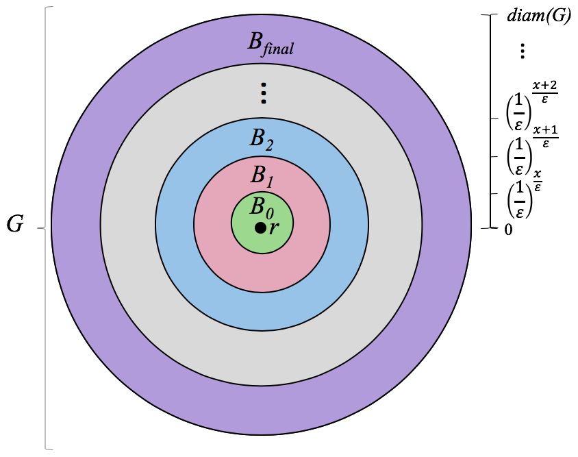
Figure 1: $G$ is divided into bands $B_{0},B_{1},...,B_{final}$ based on distance from $r$.

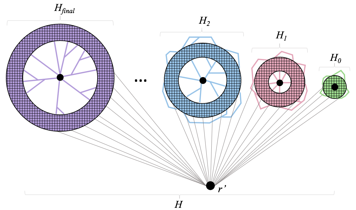
Figure 2: Each subgraph $G_{i}$ of $G$ is embedded into a host graph $H_{i}$. These graphs are joined via edges to a new depot $r^{\prime}$ to form a host graph for $G$.

Let $H^{-}$ be the graph obtained from $H$ by deleting $r^{\prime}$. The connected components of $H^{-}$ are $\{H_{i}\}_{i}$. By Lemma 1, the treewidth of each host graph $H_{i}$ is at most $(\frac{1}{\epsilon^{\prime}})^{c_{0}}$ = $(\frac{1}{\epsilon})^{c_{0}(\epsilon^{-1}+1)}$ for some constant $c_{0}$. This also bounds the treewidth of $H^{-}$. Adding a single vertex to a graph increases the treewidth by at most one, so after adding $r^{\prime}$ back, the treewidth of $H$ is $(\frac{1}{\epsilon})^{c_{0}(\epsilon^{-1}+1)}+1=(\frac{1}{\epsilon})^{c_{1}\epsilon^{-1}}$ for some constant $c_{1}$.

As for the metric approximation, it is clear that $d_{G}(u,v)\leq d_{H}(\phi(u),\phi(v))$ with probability 1. We use the following lemma to prove Equation 3.

Lemma 2.

If $\epsilon d_{G}(v,r)<d_{G}(u,r)\leq d_{G}(v,r)$, then the probability that $u$ and $v$ are in different bands is at most $\epsilon$.

Proof.

Let $i$ be the nonnegative integer such that $d_{G}(u,r)={\frac{1}{\epsilon}}^{(i+a)\frac{1}{\epsilon}}$ for some $a\in[0,1]$. Let $b$ be the number such that $d_{G}(v,r)={\frac{1}{\epsilon}}^{(i+b)\frac{1}{\epsilon}}$.

$$\frac{1}{\epsilon}\geq\frac{d_{G}(v,r)}{d_{G}(u,r)}=\frac{{\frac{1}{\epsilon}}^{(i+b)\frac{1}{\epsilon}}}{{\frac{1}{\epsilon}}^{(i+a)\frac{1}{\epsilon}}}={\frac{1}{\epsilon}}^{(b-a)\frac{1}{\epsilon}}$$

Therefore

$$b-a\leq\epsilon$$

Consider two cases. If $b\leq 1$, then the probability that $u$ and $v$ are in different bands is $Pr[a\leq x<b]\leq\epsilon$.

If $b>1$ then the probability that $u$ and $v$ are in different bands is $Pr[x\geq a\text{ or }x\leq b-1]\leq 1-a+b-1=b-a\leq\epsilon$ ∎

We now prove Equation 3. Let $u$ and $v$ be vertices in $G$. Without loss of generality, assume $d_{G}(u,r)\leq d_{G}(v,r)$. First we address the case where $d_{G}(u,r)\leq\epsilon d_{G}(v,r)$. Since $\phi(u)$ and $\phi(v)$ are both adjacent to $r^{\prime}$ in $H$, $d_{H}(\phi(u),\phi(v))\leq d_{H}(\phi(u),r^{\prime})+d_{H}(\phi(v),r^{\prime})=d_{G}(u,r)+d_{G}(v,r)\leq 2d_{G}(u,r)+d_{G}(u,v)\leq d_{G}(u,v)+2\epsilon d_{G}(v,r)$. Therefore $E[d_{H}(\phi(u),\phi(v))]\leq d_{G}(u,v)+3\epsilon[d_{G}(u,r)+d_{G}(v,r)]$

Now, suppose $d_{G}(u,r)>\epsilon d_{G}(v,r)$. If $u$ and $v$ are in the same band $B_{i}$, then by Lemma 1,

$$d_{H}(\phi(u),\phi(v)) \leq d_{H_{i}}(\phi(u),\phi(v))\leq d_{G}(u,v)+\epsilon^{\prime}\frac{1}{\epsilon}^{(i+x)\frac{1}{\epsilon}}$$

$$\leq d_{G}(u,v)+\epsilon^{\frac{1}{\epsilon}+1}4{\frac{1}{\epsilon}}^{(i+x)\frac{1}{\epsilon}}$$

$$= d_{G}(u,v)+\epsilon 4{\frac{1}{\epsilon}}^{(i+x-1)\frac{1}{\epsilon}}\leq d_{G}(u,v)+2\epsilon(d_{G}(u,r)+d_{G}(v,r))$$

In the final inequality, when $i=0$, we use the fact that all nonzero distances are at least one to give a lower bound on $d_{G}(u,r)$ and $d_{G}(v,r)$.

If $u$ and $v$ are in different bands, then since $\phi(u)$ and $\phi(v)$ are both adjacent to $r^{\prime}$ in $H$, $d_{H}(\phi(u),\phi(v))\leq d_{H}(\phi(u),r^{\prime})+d_{H}(\phi(v),r^{\prime})=d_{G}(u,r)+d_{G}(v,r)$. By Lemma 2, this case occurs with probability at most $\epsilon$.

Therefore $E[d_{H}(\phi(u),\phi(v))]\leq(d_{G}(u,v)+2\epsilon(d_{G}(u,r)+d_{G}(v,r)))+\epsilon[d_{G}(u,r)+d_{G}(v,r)]\leq d_{G}(u,v)+3\epsilon[d_{G}(u,r)+d_{G}(v,r)]$, which proves Inequality 3.

The construction does not depend on planarity only via Lemma 1. For the sake of future uses of the construction with other graph classes, we state a lemma.

Lemma 3.

Let $\mathcal{F}$ be a family of graphs closed under vertex-induced subgraphs. Suppose that there is a function $f$ and a polynomial-time algorithm that, for any graph $G$ in $\mathcal{F}$, computes a graph $H$ of treewidth at most $f(\epsilon)$ and an embedding $\phi$ of $G$ into $H$ such that, for all vertices $u$ and $v$,

$$d_{G}(u,v)\leq d_{H}(\phi(u),\phi(v))\leq d_{G}(u,v)+\epsilon D$$

Then there is a function $g$ and a randomized polynomial-time algorithm that, for any graph $G$ in $\mathcal{F}$, computes a graph $H$ with treewidth at most $g(\epsilon)$ and an embedding $\phi$ of $G$ into $H$, such that, for every pair of vertices $u,v$ of $G$, with probability 1 $d_{G}(u,v)\leq d_{H}(\phi(u),\phi(v))$, and

$$E[d_{H}(\phi(u),\phi(v))]\leq d_{G}(u,v)+\epsilon\left[(d_{G}(u,r)+d_{G}(v,r)\right]$$

4 PTAS for Capacitated Vehicle Routing

In this section, we show how to use the embedding of Section 3 to give a PTAS for Capacitated Vehicle Routing, proving Theorem 1.

4.1 Randomized algorithm

We first prove a slight relaxation of Theorem 1 in which the algorithm is randomized, and the solution value is near-optimal in expectation. We then show in Section 4.2 how to derandomize the result.

Theorem 2.

For any $\epsilon>0$ and capacity $Q$, there is a randomized algorithm for Capacitated Vehicle Routing on planar graphs that in polynomial time returns a solution whose expected value is at most $1+\epsilon$ times optimal.

Our result depends on the following lemma, which is proved in [4], the full version of [6].

Lemma 4 (Lemma 20 in [6], Lemma 15 in [4]).

Given an instance of Capacitated Vehicle Routing with capacity $Q$ on a graph $G$ with treewidth $w$, there is a dynamic-programming algorithm that finds an optimal solution in $n^{O(wQ)}$ time.

Given the dynamic program of Lemma 4 and the embedding of Theorem 2 as black boxes, the algorithm is as follows. First, the graph $G$ is embedded as in Theorem 2 using $\hat{\epsilon}=\epsilon/3Q$ into a host graph $H$ with treewidth $(\frac{1}{\hat{\epsilon}})^{c\hat{\epsilon}^{-1}}$ for some constant $c$, and $d_{G}(u,v)\leq E[d_{H}(\phi(u),\phi(v))]\leq d_{G}(u,v)+3\hat{\epsilon}(d_{G}(u,r)+d_{G}(v,r))$ for all vertices $u$ and $v$. The dynamic program of Lemma 4 is then applied to $H$. The resulting solution $SOL_{H}$ in $H$ is then mapped back to a solution $SOL_{G}$ in $G$ which is returned by the algorithm.

Note that the tours in any vehicle-routing solution can be defined by specifying the order in which clients are visited. In particular, we use $(u,v)\in SOL$ to denote that $u$ and $v$ are consecutive clients visited by the solution, noting that $u$ or $v$ may actually be the depot. In this way, a solution in $H$ is easily mapped back to a corresponding solution in $G$, as $(u,v)\in SOL_{G}$ if and only if $(\phi(u),\phi(v))\in SOL_{H}$.

We now prove Theorem 2 by analyzing this algorithm.

Lemma 5.

For any $\epsilon>0$, the algorithm described above finds a solution whose expected value is at most $1+\epsilon$ times optimal.

Proof.

Let $OPT$ be the optimal solution in $G$ and let $OPT_{H}$ be the corresponding induced solution in $H$. Since the dynamic program finds an optimal solution in $H$, we have $\text{cost}_{H}(SOL_{H})\leq\text{cost}_{H}(OPT_{H})$. Additionally, since distances in $H$ are no shorter than distances in $G$, $\text{cost}_{G}(SOL_{G})\leq\text{cost}_{H}(SOL_{H})$. Putting these pieces together, we have

$$E[\text{cost}_{G}(SOL_{G})] \leq E[\text{cost}_{H}(SOL_{H})]$$

$$\leq E[\text{cost}_{H}(OPT_{H})]$$

$$= E[\sum_{(u,v)\in OPT}d_{H}(\phi(u),\phi(v))]$$

$$= \sum_{(u,v)\in OPT}E[d_{H}(\phi(u),\phi(v))]$$

$$\leq \sum_{(u,v)\in OPT}d_{G}(u,v)+3\hat{\epsilon}(d_{G}(u,r)+d_{G}(v,r))$$

$$= \sum_{(u,v)\in OPT}d_{G}(u,v)+6\hat{\epsilon}\sum_{v\in S}d_{G}(v,r)$$

$$\leq \text{cost}_{G}(OPT)+6\hat{\epsilon}\frac{Q}{2}\text{cost}_{G}(OPT)$$

$$= (1+\epsilon)\text{cost}_{G}(OPT)$$

where the final inequality comes from Inequality 1 (see Section 1.1). ∎

The following lemma completes the proof of Theorem 2.

Lemma 6.

For any $Q,\epsilon>0$, the algorithm described above runs in polynomial time.

Proof.

By Lemma 1, computing $H$ and the embedding of $G$ into $H$ takes polynomial time. By Lemma 4, the dynamic program runs in $|V_{H}|^{O(wQ)}$ time, where $w$ is the treewidth of $H$. By Theorem 2, $w=(\frac{1}{\hat{\epsilon}})^{c\hat{\epsilon}^{-1}}=(\frac{Q}{\epsilon})^{c^{\prime}Q\epsilon^{-1}}$, where $c$ and $c^{\prime}$ are constants independent of $|V_{H}|$.

The algorithm therefore runs in $|V_{H}|^{(Q\epsilon^{-1})^{O(Q\epsilon^{-1})}}$ time. Finally, since $|V_{H}|$ is polynomial in the size of $G$, for fixed $Q$ and $\epsilon$, the running time is polynomial. ∎

4.2 Derandomization

The algorithm can be derandomized using a standard technique. The embedding of Theorem 2 partitions the vertices of the input graph into rings depending on a value $x$ chosen uniformly at random from $[0,1]$. However, the partition depends on the distances of vertices from the root $r$. It follows that the number of partitions that can arise from different choices of $x$ is at most the number of vertices. The deterministic algorithm tries each of these partitions, finding the corresponding solution, and returns the least costly of these solutions.

In particular, consider the optimum solution $OPT$. As shown in Section 4.1,

$$E[\sum_{(u,v)\in OPT}d_{H}(\phi(u),\phi(v))]$$

$$=\sum_{(u,v)\in OPT}E[d_{H}(\phi(u),\phi(v))]$$

$$\leq(1+\epsilon)\text{cost}_{G}(OPT)$$

.

Therefore, for some choice of $x$, the induced cost of $OPT$ in $H$ is nearly optimal, and the dynamic program will find a solution that costs at most as much. This completes the proof of Theorem 1.

5 Conclusion

In this paper, we present the first PTAS for Capacitated Vehicle Routing in planar graphs. Although the approximation scheme takes polynomial time, it is not an efficient PTAS (one whose running time is bounded by a polynomial whose degree is independent of the value of $\epsilon$). It is an open question as to whether an efficient PTAS exists. It is also open whether a PTAS exists when the capacity $Q$ is unbounded.

References

- [1] Tetsuo Asano, Naoki Katoh, Hisao Tamaki, and Takeshi Tokuyama. Covering points in the plane by -tours: towards a polynomial time approximation scheme for general . In Proceedings of the twenty-ninth annual ACM symposium on Theory of computing, pages 275–283. ACM, 1997.
- [2] Yair Bartal. Probabilistic approximations of metric spaces and its algorithmic applications. In 37th Annual Symposium on Foundations of Computer Science, FOCS ’96, Burlington, Vermont, USA, 14-16 October, 1996, pages 184–193, 1996.
- [3] Amariah Becker. A tight 4/3 approximation for capacitated vehicle routing in trees. In Approximation, Randomization, and Combinatorial Optimization. Algorithms and Techniques (APPROX/RANDOM 2018). Schloss Dagstuhl-Leibniz-Zentrum fuer Informatik, 2018.
- [4] Amariah Becker, Philip N. Klein, and David Saulpic. Polynomial-time approximation schemes for k-center and bounded-capacity vehicle routing in metrics with bounded highway dimension. CoRR, abs/1707.08270, 2017.
- [5] Amariah Becker, Philip N Klein, and David Saulpic. A quasi-polynomial-time approximation scheme for vehicle routing on planar and bounded-genus graphs. In LIPIcs-Leibniz International Proceedings in Informatics, volume 87. Schloss Dagstuhl-Leibniz-Zentrum fuer Informatik, 2017.
- [6] Amariah Becker, Philip N Klein, and David Saulpic. Polynomial-time approximation schemes for -center, -median, and capacitated vehicle routing in bounded highway dimension. In 26th Annual European Symposium on Algorithms (ESA 2018). Schloss Dagstuhl-Leibniz-Zentrum fuer Informatik, 2018.
- [7] Amariah Becker and Alice Paul. A ptas for minimum makespan vehicle routing in trees. arXiv preprint arXiv:1807.04308, 2018.
- [8] A. Chakrabarti, A. Jaffe, J. R. Lee, and J. Vincent. Embeddings of topological graphs: Lossy invariants, linearization, and 2-sums. In 49th Annual IEEE Symposium on Foundations of Computer Science, pages 761–770, 2008.
- [9] Nicos Christofides. Worst-case analysis of a new heuristic for the travelling salesman problem. Technical report, Carnegie-Mellon Univ Pittsburgh Pa Management Sciences Research Group, 1976.
- [10] Aparna Das and Claire Mathieu. A quasi-polynomial time approximation scheme for Euclidean capacitated vehicle routing. In Proceedings of the twenty-first annual ACM-SIAM symposium on Discrete Algorithms, pages 390–403. SIAM, 2010.
- [11] Jittat Fakcharoenphol, Satish Rao, and Kunal Talwar. A tight bound on approximating arbitrary metrics by tree metrics. J. Comput. Syst. Sci., 69(3):485–497, 2004.
- [12] A. E. Feldmann, Wai S. F., J.. Könemann, and I. Post. A (1+)-embedding of low highway dimension graphs into bounded treewidth graphs. In 42nd International Colloquium on Automata, Languages, and Programming, pages 469–480. 2015.
- [13] Eli Fox-Epstein, Philip N Klein, and Aaron Schild. Embedding planar graphs into low-treewidth graphs with applications to efficient approximation schemes for metric problems. In Proceedings of the Thirtieth Annual ACM-SIAM Symposium on Discrete Algorithms, pages 1069–1088. SIAM, 2019.
- [14] MARK Haimovich and AHG Rinnooy Kan. Bounds and heuristics for capacitated routing problems. Mathematics of operations Research, 10(4):527–542, 1985.
- [15] Michael Khachay and Roman Dubinin. PTAS for the Euclidean capacitated vehicle routing problem in . In International Conference on Discrete Optimization and Operations Research, pages 193–205. Springer, 2016.
- [16] Christos H Papadimitriou and Mihalis Yannakakis. The traveling salesman problem with distances one and two. Mathematics of Operations Research, 18(1):1–11, 1993.
- [17] K. Talwar. Bypassing the embedding: algorithms for low dimensional metrics. In 36th Annual ACM Symposium on Theory of Computing, pages 281–290, 2004.