DLocRL: A Deep Learning Pipeline for Fine-Grained Location Recognition and Linking in Tweets

Abstract.

In recent years, with the prevalence of social media and smart devices, people causally reveal their locations such as shops, hotels, and restaurants in their tweets. Recognizing and linking such fine-grained location mentions to well-defined location profiles are beneficial for retrieval and recommendation systems. In this paper, we propose DLocRL, a new deep learning pipeline for fine-grained location recognition and linking in tweets, and verify its effectiveness on a real-world Twitter dataset.

1. Introduction

Twitter is a place where users can share their daily life activities by posting tweets (i.e., short messages, up to 140 characters each). In many tweets, locations are implicitly or causally revealed by users at fine-grained granularity (Li and Sun, 2014; Ji et al., 2016; Li et al., 2017), for example, a restaurant, a shopping mall, a park or a landmark building. Here, a fine-grained location is equivalent to a point-of-interest (POI), which is a focused geographical entity (Li and Sun, 2014; Rae et al., 2012). In this paper, we target on recognizing mentions of POIs and linking these mentions to well-defined location profiles.

The two tasks are important for several reasons. First, recognizing mentions of POIs is beneficial for information retrieval (Balog, 2018). An example is that query understanding can be enhanced by exploiting POI information in location-based information retrieval systems (Espinoza et al., 2001; Schiller and Voisard, 2004). In addition, recognized POIs can be integrated into knowledge bases and support many business intelligence applications such as POI recommendation and location-aware advertising (Lingad et al., 2013; Li and Sun, 2014; Oh and Xu, 2003). Second, the linked location profile can serve as side information for the tweet, and vice versa. For example, Twitter sentiment analysis can be conducted in a more precise manner by incorporating the location profile content (Han et al., 2018).

However, recognizing POI mentions and linking these mentions to well-defined location profiles are both challenging. Due to the informal writing of tweets, POIs are usually mentioned by incomplete name, nickname, acronym or misspellings. For example, the mention vivo may refer to VivoCity which is a comprehensive shopping mall in Singapore, or a smartphone brand. Even if we have successfully recognized a POI mention, it remains challenging to link the mention to a specified location profile (i.e., a specific shopping mall with address and geo-coordinates in this case).

On the other hand, existing solutions (Han et al., 2018; Ji et al., 2016; Li and Sun, 2014) on these two tasks require a large set of features manually designed for each task and domain, which demands task and domain expertise. For example, Li et al. (Li and Sun, 2014) carefully designed lexical, grammatical, geographical and BILOU schema features (totally 11 features) to extract fine-grained locations from tweets. Ji et al. (Ji et al., 2016) proposed a joint model to recognize and link fine-grained locations from tweets with 24 hand-crafted features. Recently, Han et al. (Han et al., 2018) proposed a probabilistic model with seven types of hand-crafted features to link fine-grained location in user comments. It is now generally admitted that distributed representations could better capture lexical semantics (Goldberg, 2017). We would envision for a system that is based on distributed representations, and that can learn informative features for location recognition and linking by itself without human effort.

In this paper, we propose DLocRL, a new Deep pipeline for fine-grained Location Recognition and Linking in tweets. DLocRL is designed to adopt effective representation learning, semantic composition, and attention and gate mechanisms to exploit the multiple semantic context features for location recognition and linking. DLocRL consists of two core modules: recognition module and linking module.

The recognition module aims to extract a text segment referring to a fine-grained location (i.e., POI) from a given tweet. In DLocRL, we formulate the recognition task as a sequence labeling problem (i.e., assigning tags to tokens in the given sequence). We adopt bi-directional long short-term memory with conditional random fields output layer (BiLSTM-CRF) to train a POI recognizer.

The linking module aims to link each recognized POI to a corresponding location profile. Before linking POIs to location profiles, an extensive collection of location profiles (CLP) is constructed. Given an input pair $\langle$POI, Profile$\rangle$, the linking module is trained to judge whether the location profile corresponds to the POI. More specifically, DLocRL utilizes two pairs of parallel LSTMs to encode the left context and right context for a POI, respectively. The location profiles are represented by their constituents with TF-IDF weights and one-hot schema. The Manhattan distance is used to measure the geographical distances between users and profiles. Finally, the representation of $\langle$POI, Profile$\rangle$ comes from three sources: tweet-level contextual information, location profile representation and geographical distance. The representation is then fed into a fully-connected layer for final linking prediction. Moreover, to take advantage of the geographical coherence information among mentioned POIs in the same tweet, we develop Geographical Pair Linking (Geo-PL), a post-processing strategy to further enhance the linking accuracy.

In summary, we make the following contributions: (1) We propose DLocRL, a new deep learning pipeline for fine-grained Location Recognition and Linking in tweets. To the best of our knowledge, our work is the first attempt to address location recognition and linking in the paradigm of deep learning. (2) We develop the Geographical Pair Linking (Geo-PL) approach, a post-processing strategy to further improve linking performance. (3) We conduct extensive experiments on a real-world Twitter dataset. The experimental results show the effectiveness of DLocRL on fine-grained location recognition and linking. We also conduct ablation studies to validate the effectiveness of each design choice.

2. Related work

2.1. Location Mention Recognition and Disambiguation

Recognition. Facing noisy and short tweets, traditional NER methods suffer from their unreliable linguistic features (Zheng et al., 2018). Prior solutions exploit comprehensive linguistic features like Part-of-Speech tags, capitalization (Ratinov and Roth, 2009), Brown clustering (Brown et al., 1992) to improve recognition performance. For example, Li et al. (Li and Sun, 2014) carefully designed lexical, grammatical, geographical and BILOU schema features (totally 11 features) to extract fine-grained locations from tweets. Ji et al. (Ji et al., 2016) proposed a joint model to recognize and link fine-grained locations from tweets with 24 hand-crafted features. Zhang et al. (Zhang and Gelernter, 2014) designed four types of features and trained a classifier to select the best match among gazetteer candidates. Generally, location gazetteers are widely used in location mention recognition (Malmasi and Dras, 2015; Zhang and Gelernter, 2014; Li and Sun, 2014). For noisy text, Malmasi et al. (Malmasi and Dras, 2015) proposed an approach based on Noun Phrase extraction and n-gram based matching instead of the traditional methods using NER or CRF. Different from these existing works, our approach DLocRL does not require hand-crafted features.

Disambiguation. For entity disambiguation, many studies attempt to exploit the coherence among mentioned entities. Pair-wise (Kulkarni et al., 2009) and global collective methods (Hoffart et al., 2011; Han et al., 2011; Tsochantaridis et al., 2005) have been applied to explore the coherence. Zhang et al. (Zhang and Gelernter, 2014) and Ji et al. (Ji et al., 2016) observed that the geographical coherence is effective in location disambiguation task. Also, instead of tweet-level coherence, Li et al. (Li et al., 2014) utilized user-level coherence to facilitate entity disambiguation. Besides, Shen et al. (Shen et al., 2013) introduced user interest modeling to collective disambiguation.

To form an entirely end-to-end model for joint recognition and linking, Guo et al. (Guo et al., 2013) and Ji et al. (Ji et al., 2016) adopted structural SVM and perceptron, respectively. Furthermore, the beam search algorithm (Zhang and Clark, 2008) is also used in (Ji et al., 2016) to search the best combination of the mention recognition and linking. In this work, we devise DLocRL, a new pipeline which can be upgraded and optimized much easier than previous joint models and still achieves better performance.

2.2. Neural Networks for NER and EL

Named Entity Recognition (NER). The use of neural models for NER was pioneered by Collobert et al. (Collobert et al., 2011), where an architecture based on temporal convolutional neural networks (CNNs) over word sequence was proposed. Chiu et al. (Chiu and Nichols, 2016) utilized CNN to detect character-level features and LSTM to capture the word-level context in a sentence. Yang et al. (Yang et al., 2016) proposed a gated recurrent unit (GRU) network to learn useful morphological representation from the character sequence of a word. Recently, Peters et al. (Peters et al., 2018) proposed deep contextualized word representation, which can model syntax, semantics, and polysemy. Akbik et al. (Akbik et al., 2018) proposed contextual string embeddings, to leverage the internal states of a trained character language model to produce a novel type of word embedding.

Entity Linking (EL). Neural networks were firstly used for entity linking by Sun et al. (Sun et al., 2015). They proposed a model which takes consideration of the semantic representations of mention, context, and entity. Recently, Phan et al. (Phan et al., 2017) proposed a neural network for entity linking with LSTM and attention mechanism. They also proposed Pair Linking to enhance collective linking by measuring the cosine similarity of the text embeddings between two mentioned entities.

3. Model Description

Figure 1 shows the workflow of DLocRL, which consists of recognition module and location linking module.

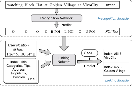
Figure 1. A running example to illustrate the workflow of DLocRL.

3.1. Location Recognition

Figure 2 shows the architecture of the location recognition module. The representation of a word consists of its pre-trained word embedding, BILOU pre-label and character-level representation. Finally, BiLSTM-CRF is utilized to infer tag sequence based on the representations.

Pre-trained Word Embedding. To deal with the problem of informal spellings and casual expressions, we should capture the information from tweets as accurate as possible. We use the GloVe(Pennington et al., 2014) embeddings pre-trained on a large-scale Twitter corpus of two billion tweets. The vocabulary of pre-trained embeddings covers most common misspellings and aliases of most common words.

Pre-label. POI inventory, containing partial and familiar names from Foursquare, is proposed in (Li and Sun, 2014) to pre-label candidate location mentions in tweets. It has been proved that pre-label is an essential resource to improve recognition performance. We use a CRF toolkit to automatically assign the pre-labels with BILOU scheme(Ratinov and Roth, 2009).

Character-level Representation. Previous studies (Chiu and Nichols, 2016; Huang et al., 2015) have shown that character-level information (e.g., prefix and suffix of a word) is an effective resource for NER task. CNN and BiLSTM are commonly used in previous works to extract character-level representation. In our model, we use CNN because of its lower computational cost (Chiu and Nichols, 2016; Li et al., 2018).

BiLSTM-CRF. LSTM is a variant of recurrent neural network (RNN) and is designed to deal with vanishing gradients problem. BiLSTM uses two LSTMs to represent each token of the sequence based on both the past and the future context of the token. As shown in Figure 2, one LSTM processes the sequence from left to right, the other one from right to left. For a word, we concatenate its pre-trained word embedding, pre-label and character-level representation as its final representation, which is then fed into a BiLSTM layer. Then, the output sequence is fed into a CRF layer to infer the tag sequence. BiLSTM-CRF is a state-of-the-art approach to named entity recognition (Huang et al., 2015; Dyer et al., 2015).

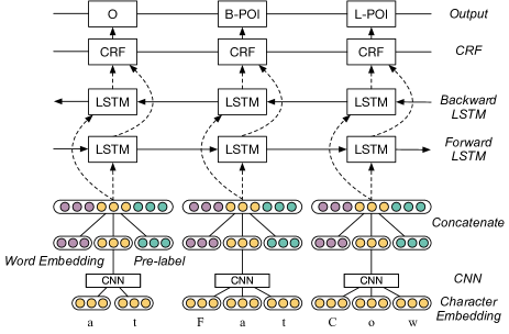
Figure 2. The architecture of location recognition module.

3.2. Location Linking

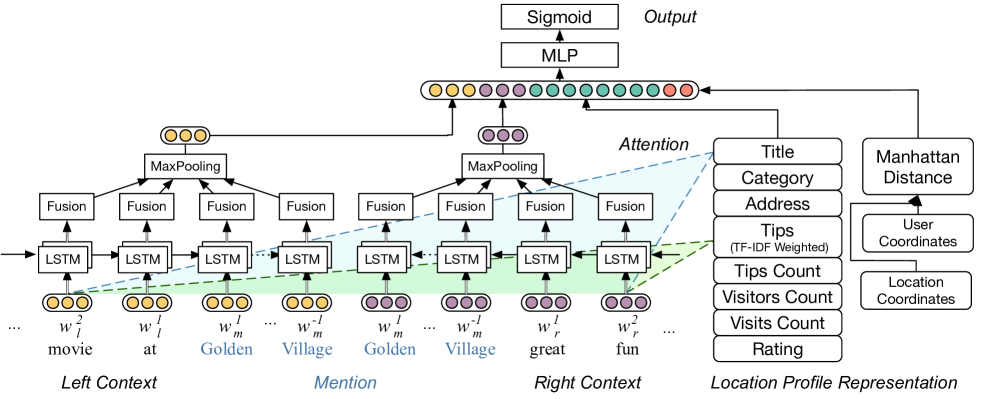
Figure 3. The architecture of location linking network. The input is a pair $\langle$tweet, profile$\rangle$, and the output is the matching score.

Figure 3 shows the architecture of the location linking module. We use two pairs of parallel LSTMs (four in total) to encode the left-side and right-side contexts of a mention, respectively. Note that the input of the two parallel LSTMs for each side is re-weighted by two different attentions from the location profile. The output sequences of LSTMs are “fused” by a fusion gate and then fed into a max-pooling layer over all time steps as the final representation for each side context. Next, we concatenate the left-side context representation, right-side context representation, the representation of location profile together with the Manhattan distance between user coordinates (i.e., user position attached to the tweet) and coordinates from location profile. Finally, a multilayer perceptron (MLP) with a sigmoid activated output layer is used to output a scalar ranged between zero and one as the matching score.

Location Profile Mapping Dictionary. Following (Ji et al., 2016), we use a location profile mapping dictionary to recall all possible candidates for a location mention. The key of the dictionary is a possible POI mention, and the value is the list of candidate profile indexes for the POI mention. If the mention is not in the mapping dictionary, we predict it as un-linkable. The dictionary is constructed with Foursquare check-in tweets.

Mention’s Context. Following (Phan et al., 2017), we use LSTM networks to capture two-side contextual information of the POI mention. The difference is that we use all words in a tweet instead of specific window size. The left-side context starts from the leftmost word in a tweet and ends at the rightmost word inside the mention. Conversely, the right-side context starts from the tweet’s rightmost word and ends at the leftmost word of the mention. Since the tweet does not have a long context, we use all words to understand the tweet as a whole. Note that the input of LSTM layers is re-weighted with a multi-attention mechanism, which is to be detailed shortly.

Behavioral and Semantic Information. Users often reveal their locations and describe what they are doing in tweets. For example, a user posts “Great lobster @ Red Robin!”, which contains information about behavior (having lobster). Here, we name such information as behavioral information. Obviously, since few restaurants serve lobster, it could be beneficial for POI disambiguation. According to our observation, tweets share the same behavioral information with the tips (i.e., user comments) in the Foursquare location profile. On the other hand, some words in a tweet may be directly semantically relevant to the category or address of a location. For instance, in the tweet “Best wine at Elle’s in the center”, wine is closer to bar in word embedding space. Such information is beneficial for location disambiguation between Elle’s Bar and Elle’s Salon. Similarly, in the same example, center is a synonym for Central Region. This can be helpful for picking a location profile titled “Elle’s Bar - Central Region” out of other branches of Elle’s Bar. We name such information as semantic information.

Multi-attention Mechanism. To comprehensively exploit semantic information and behavioral information, we develop a multi-attention mechanism to assign weights for the input sequence. As shown in Figure 3, we use the title representation and tips representation as two attention vectors. Specifically, given an input word embedding $w_{i}$ in a tweet and an attention vector $p$ (i.e., representation of title or tips from location profile), the re-weighted input word embedding $w^{\prime}_{i}$ is defined by:

(1) $$z_{i}=\tanh{(V_{p}p+V_{w}w_{i})}$$

(2) $$s_{i}=\operatorname*{softmax}(v_{k}z_{i}+v_{b})$$

(3) $$w^{\prime}_{i}=w_{i}s_{i}$$

where $V_{*}$, $v_{k}$, and $v_{b}$ are attention parameters which can be learned during training. The TF-IDF weighted tips representation (to be detailed shortly) contains the most characteristic behavioral information about a location. Thus, the attention from tips can highlight the parts which are most relevant with the tips. Similarly, the title contains rich semantic information (including location name, branch name and business status) which can highlight the parts relevant to the location.

Fusion Gate. To collect important information from the output of two parallel LSTMs, we borrow a simple but practical fusion gate from (Shen et al., 2018). Given the output of two parallel LSTMs with different attentions (i.e., $x^{1}_{i}$ and $x^{2}_{i}$), the output of fusion gate $u_{i}$ is formally defined by:

(4) $$f_{i}=\operatorname*{sigmoid}(W_{1}x^{1}_{i}+W_{2}x^{2}_{i}+b)$$

(5) $$u_{i}=f_{i}\odot x^{1}_{i}+(1-f_{i})\odot x^{2}_{i}$$

where $W_{1}$, $W_{2}$, and $b$ are learnable parameters. The fusion gate enables the model to learn how to weight the two input sequences, which solves the problem of the imbalanced importance of behavioral information and semantic information.

Location Profile. The properties (exclude “category” ) of a location profile fall into two classes: word-based and numeric-based. For word-based properties (i.e., title, address, and tips), we represent each property by averaging all word embeddings inside it. In particular, the word embeddings of “tips” are weighted by TF-IDF schema. For numeric-based properties (i.e., tips count, visitors count and visits count), we normalize them through the whole CLP. For category property, we encode it as a one-hot vector. Finally, we concatenate representations of all properties together as the location profile representation.

Manhattan Distance. To measure the distance between user coordinates and location coordinates in a city, we use the Manhattan distance (i.e., taxicab distance) defined by:

(6) $$d(p,q)=\lvert p_{x}-q_{x}\rvert+\lvert p_{y}-q_{y}\rvert$$

where $p$ and $q$ are two pairs of coordinates. Manhattan distance is better than Euclidean distance since the road network in a city or suburb is usually orthogonal. Note that not every tweet has an attached user position. For these situations, we fix the distance value to a pre-defined constant. Manhattan distance is also used in our post-processing, geographical pair linking, which will be discussed in Section 4.

Final Prediction. For all candidate location profiles in our mapping dictionary for a mention, we predict the matching score between the mention and each candidate. Formally, the final predicted location profile $p_{i}$ for mention $m_{i}$ is computed by:

(7) $$p_{i}=\operatorname*{arg\,max}\limits_{p_{j}\in c(m_{i})}\phi(m_{i},p_{j})$$

where $c(m_{i})$ is the candidate set for $m_{i}$ and $\phi(m_{i},p_{j})$ is the matching score between $m_{i}$ and $p_{j}$.

4. Geographical Pair Linking

In this section, we introduce Geographical Pair Linking (Geo-PL), a post-processing strategy to enhance our linking performance.

For location linking, one of the most valuable information is the geographical coherence among mentioned locations in the same tweet. First, instead of directly calling the branch name of a chain restaurant, users are more likely to mention them with another location (usually a landmark). Second, people may describe a route by listing the locations along the way one by one, which also reveals the coherence among the mentioned locations.

For geographical coherence, prior studies often measure the distances among all mentions in a tweet. According to our observation, geographical coherence between two locations is strong enough for location disambiguation. Moreover, as illustrated in Figure 4, when a user mentions four locations with a conventional way like “Had dinner at A near B then saw a movie at C in D,” the geographical coherence measurement among all mentions brings obvious error. It obtains the collective minimum but disregards the strong connection between two mentions.

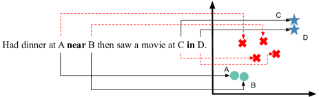
Figure 4. A wrong case of taking into account the coherence among all mentions. A, B, C and D are true POIs mentioned by a user. The incorrect predictions are marked with red dashed arrows and crosses.

Table 1. Performance on Location Recognition and Location Linking.

Methods	Location Recognition			Location Linking			Recognition + Linking
	Pr	Re	$F_{1}$	Pr	Re	$F_{1}$	Pr	Re	$F_{1}$
Li et al. (Li and Sun, 2014)	0.8962	0.7661	0.8261	-	-	-	-	-	-
Shen et al. (Shen et al., 2013)	-	-	-	0.6723	0.6349	0.6531	-	-	-
Pipelined (Li and Sun, 2014) (Shen et al., 2013)	-	-	-	-	-	-	0.6339	0.5635	0.5966
$\rm JoRL_{L}$ (Ji et al., 2016)	0.8926	0.7823	0.8338	-	-	-	0.8152	0.5952	0.6881
DLocRL	0.8575	0.8091	0.8326	0.8235	0.7778	0.8000	0.8350	0.6825	0.7511

To exploit pair-wise geographical coherence, we developed Geographical Pair Linking (Geo-PL) algorithm based on the Pair Linking algorithm (Phan et al., 2017). The original algorithm measures the cosine similarity between text embeddings, while we use Manhattan distance discussed in Section 3.2 to measure the geographical coherence. Geo-PL iteratively resolves all pairs of mentions, starting from the most confident pair. The confidence score of a pair of links $m_{i}\mapsto p_{i}$ and $m_{j}\mapsto p_{j}$ is defined by:

(8) $$conf(i,j)=(1-\beta)\frac{[\phi(m_{i},p_{i})+\phi(m_{j},p_{j})]}{2}+\beta\frac{1}{d(p_{i},p_{j})}$$

where $\beta$ is a given coefficient representing the preference between the matching scores and the geographical coherence; $d$ is the Manhattan distance defined by Equation 6. In the case of $p_{i}=p_{j}$, we temporarily set $\beta$ to 0 when calculating. The procedure of Geo-PL (the same as Pair Linking) is detailed in Algorithm 1. Note that if there is only one POI mention in a tweet, we simply predict its location profile by Equation 7.

Input: N mentions($m_{1},...,m_{N}$). Mention $m_{i}$ has candidate profiles $\{e|e_{i}\in C(m_{i})\}$

Output: $\Gamma=(p_{1},...,p_{N})$

1$p_{i}\leftarrow null,\forall p_{i}\in\Gamma$;

2 foreach $pair(m_{i},m_{j})\land m_{i}\not=m_{j}$ do

3       $Q_{m_{i},m_{j}}\leftarrow top\_pair(m_{i},C(m_{i}),m_{j},C(m_{j}))$;

4       $Q.add(Q_{m_{i},m_{j}})$;

5      

6 end foreach

7while $\exists p_{i}\in\Gamma,p_{i}=null$ do

8       $(m_{i},e_{i},m_{j},e_{j})\leftarrow most\_confident\_pair(Q)$;

9       $p_{i}\leftarrow e_{i}$;

10       $p_{j}\leftarrow e_{j}$;

11       for $k:=1\to N\land p_{k}=null$ do

12             $Q_{m_{k},m_{i}}\leftarrow top\_pair(m_{k},C(m_{k}),m_{i},\{p_{i}\})$;

13             $Q_{m_{k},m_{j}}\leftarrow top\_pair(m_{k},C(m_{k}),m_{j},\{p_{j}\})$;

14            

15       end for

16      

17 end while

Algorithm 1 Geo-PL Algorithm

5. Experiment

5.1. Data Preparation

We use a Singaporean national Twitter dataset released by Ji et al. (Ji et al., 2016). The dataset includes a CLP and a set of labeled tweets.

326,853 Foursquare check-in tweets, containing both formal auto-generated POI name and informal user mentions, are collected to build the CLP (including 22,414 valid location profiles) and the POI inventory (including 27,386 entries). Location profile mapping dictionary (see Section 3.2) is also constructed with check-in tweets. Informal mentions in check-in tweets and the indexes of crawled profiles are used as keys and values, respectively. The final location profile mapping dictionary has 24,750 keys and 63,091 ¡key, value¿ mappings.

The dataset consists of 3,611 labeled tweets and 1,542 POI locations, 543 of which can be linked to a profile in the CLP. 10% of tweets have an attached user position. These tweets are labeled by human annotators. All possible POI mentions are labeled with one of NPOI (i.e., not a POI mention), index of linked location profile, or NIL (i.e., cannot be linked to a profile).

We split the 3,611 labeled tweets randomly into three subsets: 2,500 tweets for training, 211 tweets for validation, and 900 tweets for testing. Same POI inventory and location profile mapping dictionary used in (Ji et al., 2016) are employed through all models in our experiments.

5.2. Parameter Setting and Evaluation Metrics

We set $\beta$, the coefficient of Geo-PL preference to 0.8 based on fine-tuning on the validation set. When concatenating the scalars to be the input of MLP, we duplicate them to the same number of dimensions as the word-based properties (i.e., 200 dimensions in our experiments). This setting prevents the scalars from being “ignored” during training.

We conduct experiments on location recognition subtask, location linking subtask and the whole task, respectively. We adopt three metrics, Precision ($Pr$), Recall ($Re$) and $F_{1}$ which are widely used to evaluate NER and EL tasks. In particular, we use the ground-truth mentions instead of the predicted output of the recognition module, to get the metric scores for location linking.

5.3. Overall Comparison

We compare our model with state-of-the-art solutions. More specifically, we compare our model with (Li and Sun, 2014) and (Ji et al., 2016) for recognition, and (Shen et al., 2013) for linking, respectively. Note that the performance of (Ji et al., 2016) on linking subtask is not provided since it is a joint model. For the whole task, we choose $\rm JoRL_{L}$ as the baseline since it is the state-of-the-art joint model in supervised learning manner. All models are fine-tuned on the validation set.

The result is shown in Table 1. We observe that DLocRL achieves the highest recall on location recognition. DLocRL beats Li et al. (Li and Sun, 2014) and $\rm JoRL_{L}$ (Ji et al., 2016) with relative recall improvements of $5.61\%$ and $3.43\%$, respectively. We contribute this to the fact that word/character embeddings enable our model to be more “tolerant” than prior works which depend on hand-crafted features. Although the precision score of DLocRL is not good, it does not have an impact on the whole task, because the location profile mapping dictionary can filter out most false positive (FP) prediction in the linking module.

On location linking subtask, our method outperforms the work (Shen et al., 2013) by 22.49% on precision, 22.51% on recall and 22.49% on $F_{1}$.

On the whole task, our model prominently outperforms the state-of-the-art joint solution ($\rm JoRL_{L}$) on all three metrics (2.43% on precision, 14.67% on recall, 9.16% on $F_{1}$). Also, our model dramatically outperforms the prior state-of-the-art pipeline by 31.72% on precision, 21.12% on recall and 25.90% on $F_{1}$.

5.4. Effect of Multi-attention for Linking

We conduct experiments to verify the effectiveness of the multi-attention mechanism. Table 2 shows the linking performance with single attention from tips/title attentions and multi-attention. Note that the single attention approaches can only slightly improve the performance because they have “prejudice” which considers either behavioral information or semantic information. By “fusing” this two information, DLocRL eliminates the prejudice so it can effectively filter out noisy information. With the multi-attention mechanism, DLocRL improves the performance of linking module by 4.25% on precision, 4.26% on recall, and 4.26% on $F_{1}$, compared with the baseline.

5.5. Effect of Geo-PL for Linking

As discussed in Section 4, we introduce a novel post-processing strategy, named Geo-PL. Here, we conduct experiments to show the impact of Geo-PL for location linking. Table 3 shows the experimental results. Compared with no Geo-PL component, DLocRL (with Geo-PL) significantly improves precision by 13.46%, recall by 8.89% and $F_{1}$ by 11.11%.

Table 2. Effect of Multi-attention Mechanism for Linking.

Attention	Location Linking
	Pr	Re	$F_{1}$
Baseline (without attention)	0.7899	0.7460	0.7673
Single Tips Attention	0.7983	0.7540	0.7755
Single Title Attention	0.7899	0.7460	0.7673
Tips + Title (multi-attention)	0.8235	0.7778	0.8000

Table 3. Effect of Geo-PL for Linking.

Strategy	Location Linking
	Pr	Re	$F_{1}$
Without Geo-PL	0.7258	0.7143	0.7200
With Geo-PL	0.8235	0.7778	0.8000

6. Conclusions

In this paper, we introduce DLocRL, the first deep neural network based pipeline to recognize fine-grained location mentions in tweets and link the recognized locations to location profiles. Moreover, we develop a novel post-processing strategy which can further improve location linking performance. Through extensive experiments, we demonstrate the effectiveness of DLocRL against state-of-the-art solutions on a real-world Twitter dataset. The ablation experiments show the effectiveness of multi-attention mechanism and Geo-PL strategy on location linking.

- (1)
- Akbik et al. (2018) Alan Akbik, Duncan Blythe, and Roland Vollgraf. 2018. Contextual String Embeddings for Sequence Labeling. In Proc. COLING. 1638–1649.
- Balog (2018) Krisztian Balog. 2018. Entity-Oriented Search. (2018).
- Brown et al. (1992) Peter F. Brown, Vincent J. Della Pietra, Peter V. de Souza, Jennifer C. Lai, and Robert L. Mercer. 1992. Class-Based n-gram Models of Natural Language. Computational Linguistics 18, 4 (1992), 467–479.
- Chiu and Nichols (2016) Jason PC Chiu and Eric Nichols. 2016. Named entity recognition with bidirectional LSTM-CNNs. In TACL, Vol. 4. 357–370.
- Collobert et al. (2011) Ronan Collobert, Jason Weston, Léon Bottou, Michael Karlen, Koray Kavukcuoglu, and Pavel Kuksa. 2011. Natural language processing (almost) from scratch. Journal of Machine Learning Research 12, Aug (2011), 2493–2537.
- Dyer et al. (2015) Chris Dyer, Miguel Ballesteros, Wang Ling, Austin Matthews, and Noah A. Smith. 2015. Transition-Based Dependency Parsing with Stack Long Short-Term Memory. In Proc ACL. 334–343.
- Espinoza et al. (2001) Fredrik Espinoza, Per Persson, Anna Sandin, Hanna Nyström, Elenor Cacciatore, and Markus Bylund. 2001. Geonotes: Social and navigational aspects of location-based information systems. In Proc. UBICOMP. 2–17.
- Goldberg (2017) Yoav Goldberg. 2017. Neural network methods for natural language processing. Synthesis Lectures on Human Language Technologies 10, 1 (2017), 1–309.
- Guo et al. (2013) Stephen Guo, Ming-Wei Chang, and Emre Kiciman. 2013. To Link or Not to Link? A Study on End-to-End Tweet Entity Linking. In Proc. NAACL-HLT. 1020–1030.
- Han et al. (2018) Jialong Han, Aixin Sun, Gao Cong, Wayne Xin Zhao, Zongcheng Ji, and Minh C Phan. 2018. Linking Fine-Grained Locations in User Comments. IEEE Transactions on Knowledge and Data Engineering 30, 1 (2018), 59–72.
- Han et al. (2011) Xianpei Han, Le Sun, and Jun Zhao. 2011. Collective entity linking in web text: a graph-based method. In Proc. SIGIR. 765–774.
- Hoffart et al. (2011) Johannes Hoffart, Mohamed Amir Yosef, Ilaria Bordino, Hagen Fürstenau, Manfred Pinkal, Marc Spaniol, Bilyana Taneva, Stefan Thater, and Gerhard Weikum. 2011. Robust Disambiguation of Named Entities in Text. In Proc. EMNLP. 782–792.
- Huang et al. (2015) Zhiheng Huang, Wei Xu, and Kai Yu. 2015. Bidirectional LSTM-CRF models for sequence tagging. arXiv preprint arXiv:1508.01991 (2015).
- Ji et al. (2016) Zongcheng Ji, Aixin Sun, Gao Cong, and Jialong Han. 2016. Joint Recognition and Linking of Fine-Grained Locations from Tweets. In Proc. WWW. 1271–1281.
- Kulkarni et al. (2009) Sayali Kulkarni, Amit Singh, Ganesh Ramakrishnan, and Soumen Chakrabarti. 2009. Collective annotation of Wikipedia entities in web text. In Proc. SIGKDD. 457–466.
- Li and Sun (2014) Chenliang Li and Aixin Sun. 2014. Fine-grained location extraction from tweets with temporal awareness. In Proc. SIGIR. 43–52.
- Li et al. (2017) Daifeng Li, Zhipeng Luo, Ying Ding, Jie Tang, Gordon Guo-Zheng Sun, Xiaowen Dai, John Du, Jingwei Zhang, and Shoubin Kong. 2017. User-level microblogging recommendation incorporating social influence. Journal of the Association for Information Science and Technology 68, 3 (2017), 553–568.
- Li et al. (2014) Guoliang Li, Jun Hu, Jianhua Feng, and Kian-Lee Tan. 2014. Effective location identification from microblogs. In Proc. ICDE. 880–891.
- Li et al. (2018) Jing Li, Aixin Sun, and Shafiq Joty. 2018. SegBot: A Generic Neural Text Segmentation Model with Pointer Network. In Proc. IJCAI. 4166–4172.
- Lingad et al. (2013) John Lingad, Sarvnaz Karimi, and Jie Yin. 2013. Location extraction from disaster-related microblogs. In Proc. WWW. 1017–1020.
- Malmasi and Dras (2015) Shervin Malmasi and Mark Dras. 2015. Location Mention Detection in Tweets and Microblogs. In Proc. PACLING. 123–134.
- Oh and Xu (2003) Lih-Bin Oh and Heng Xu. 2003. Effects of multimedia on mobile consumer behavior: An empirical study of location-aware advertising. Proc. ICiS (2003), 56.
- Pennington et al. (2014) Jeffrey Pennington, Richard Socher, and Christopher D. Manning. 2014. Glove: Global Vectors for Word Representation. In Proc. EMNLP. 1532–1543.
- Peters et al. (2018) Matthew E Peters, Mark Neumann, Mohit Iyyer, Matt Gardner, Christopher Clark, Kenton Lee, and Luke Zettlemoyer. 2018. Deep contextualized word representations. In Proc. NAACL-HLT. 2227–2237.
- Phan et al. (2017) Minh C. Phan, Aixin Sun, Yi Tay, Jialong Han, and Chenliang Li. 2017. NeuPL: Attention-based Semantic Matching and Pair-Linking for Entity Disambiguation. In Proc. CIKM. 1667–1676.
- Rae et al. (2012) Adam Rae, Vanessa Murdock, Adrian Popescu, and Hugues Bouchard. 2012. Mining the web for points of interest. In Proc. SIGIR. 711–720.
- Ratinov and Roth (2009) Lev-Arie Ratinov and Dan Roth. 2009. Design Challenges and Misconceptions in Named Entity Recognition. In Proc. CoNLL. 147–155.
- Schiller and Voisard (2004) Jochen Schiller and Agnès Voisard. 2004. Location-based services. Elsevier.
- Shen et al. (2018) Tao Shen, Tianyi Zhou, Guodong Long, Jing Jiang, Shirui Pan, and Chengqi Zhang. 2018. DiSAN: Directional Self-Attention Network for RNN/CNN-Free Language Understanding. In Proc. AAAI.
- Shen et al. (2013) Wei Shen, Jianyong Wang, Ping Luo, and Min Wang. 2013. Linking named entities in Tweets with knowledge base via user interest modeling. In Proc. SIGKDD. 68–76.
- Sun et al. (2015) Yaming Sun, Lei Lin, Duyu Tang, Nan Yang, Zhenzhou Ji, and Xiaolong Wang. 2015. Modeling Mention, Context and Entity with Neural Networks for Entity Disambiguation. In Proc. IJCAI. 1333–1339.
- Tsochantaridis et al. (2005) Ioannis Tsochantaridis, Thorsten Joachims, Thomas Hofmann, and Yasemin Altun. 2005. Large Margin Methods for Structured and Interdependent Output Variables. Journal of Machine Learning Research 6 (2005), 1453–1484.
- Yang et al. (2016) Zhilin Yang, Ruslan Salakhutdinov, and William Cohen. 2016. Multi-task cross-lingual sequence tagging from scratch. arXiv preprint arXiv:1603.06270 (2016).
- Zhang and Gelernter (2014) Wei Zhang and Judith Gelernter. 2014. Geocoding location expressions in Twitter messages: A preference learning method. J. Spatial Information Science 9, 1 (2014), 37–70.
- Zhang and Clark (2008) Yue Zhang and Stephen Clark. 2008. Joint Word Segmentation and POS Tagging Using a Single Perceptron. In Proc. ACL. 888–896.
- Zheng et al. (2018) Xin Zheng, Jialong Han, and Aixin Sun. 2018. A Survey of Location Prediction on Twitter. IEEE Trans. Knowl. Data Eng. 30, 9 (2018), 1652–1671.