Distributed Nesterov gradient methods
over arbitrary graphs

Abstract

In this letter, we introduce a distributed Nesterov method, termed as $\mathcal{ABN}$, that does not require doubly-stochastic weight matrices. Instead, the implementation is based on a simultaneous application of both row- and column-stochastic weights that makes this method applicable to arbitrary (strongly-connected) graphs. Since constructing column-stochastic weights needs additional information (the number of outgoing neighbors at each agent), not available in certain communication protocols, we derive a variation, termed as FROZEN, that only requires row-stochastic weights but at the expense of additional iterations for eigenvector learning. We numerically study these algorithms for various objective functions and network parameters and show that the proposed distributed Nesterov methods achieve acceleration compared to the current state-of-the-art methods for distributed optimization.

I Introduction

Distributed optimization has recently seen a surge of interest particularly with the emergence of modern signal processing and machine learning applications. A well-studied problem in this domain is finite sum minimization that also has some relevance to empirical risk formulations, i.e.,

$$\min_{\mathbf{x}}\sum_{i}f_{i}(\mathbf{x}),$$

where each $f_{i}:\mathbb{R}^{p}\rightarrow\mathbb{R}$ is a smooth and convex function available at an agent $i$. Since the $f_{i}$’s depend on data that may be private to each agent and communicating large data is impractical, developing distributed solutions of the above problem have attracted a strong interest. Related work has been a topic of significant research in the areas of signal processing and control [1, 2, 3, 4], and more recently has also found coverage in the machine learning literature [5, 6, 7, 8, 9, 10].

Since the focus is on distributed implementation, the information exchange mechanism among the agents becomes a key ingredient of the solutions. Such inter-agent information exchange is modeled by a graph and significant work has focused on algorithm design under various graph topologies. The associated algorithms require two key steps: (i) consensus, i.e., reaching agreement among the agents; and, (ii) optimality, i.e., showing that the agreement is on the optimal solution. Naturally, consensus algorithms have been predominantly used as the basic building block of distributed optimization on top of which a gradient correction is added to steer the agreement to the optimal solution. Initial work thus follows closely the progress achieved in the consensus algorithms and extensions to various graph topologies, see e.g., [11, 12, 13, 5, 6, 14, 15].

Early work on consensus assumes doubly-stochastic (DS) weights [16, 17], which require the underlying graphs to be undirected (or balanced) since both incoming and outgoing weights must sum to $1$. The subsequent work on optimization over undirected graphs includes [12] where the convergence is sublinear and [18, 19, 20] with linear convergence. For directed (and unbalanced) graphs, it is not possible to construct DS weights, i.e., the weights can be chosen such that they sum to $1$ either only on incoming edges or only on outgoing edges. Optimization over digraphs [21, 22, 23, 24, 25, 26, 27, 28] thus has been built on consensus with non-DS weights [29, 30, 31]. Required now is a division with additional iterates that learn the non-$\mathbf{1}$ (where $\mathbf{1}$ is a vector of all $1$’s) Perron eigenvector of the underlying weight matrix, see [23, 25, 26] for details. Such division causes significant conservatism and stability issues [32].

Recently, we introduced the $\mathcal{AB}$ algorithm that removes the need of eigenvector learning by utilizing both row-stochastic (RS) and column-stochastic (CS) weights, simultaneously, [33]. The algorithm thus is applicable to arbitrary strongly-connected graphs. The intuition behind using both sets of weights is as follows: Let $A$ be RS and $B$ be CS, with $\mathbf{w}^{\top}A=\mathbf{w}^{\top}$ and $B\mathbf{v}=\mathbf{v}$, in addition to being primitive. From Perron-Frobenius theorem, we have that $A^{\infty}=\mathbf{1}\mathbf{w}^{\top}$ and $B^{\infty}=\mathbf{v}\mathbf{1}^{\top}$. Clearly, using $A$ or $B$ alone makes an algorithm dependent on the non-$\mathbf{1}$ Perron eigenvector ($\mathbf{w}$ or $\mathbf{v}$) and thus the need for the aforementioned division by the iterates learning this eigenvector. Using $A$ and $B$ simultaneously, the asymptotics of $\mathcal{AB}$ are driven by, loosely speaking, $A^{\infty}B^{\infty}=(\mathbf{w}^{\top}\mathbf{v})\cdot\mathbf{1}\mathbf{1}^{\top}$, which recovers the consensus matrix, $\mathbf{1}\mathbf{1}^{\top}$, without any scaling. It is shown in [33] that $\mathcal{AB}$ converges linearly to the optimal for smooth and strongly-convex functions.

In this letter, we study accelerated optimization over arbitrary graphs by extending $\mathcal{AB}$ with Nesterov’s momentum. We first propose $\mathcal{ABN}$ that uses both RS and CS weights. Construct CS weights requires each agent to know at least its out-degree, which may not be possible in broadcast-type communication scenarios. To address this challenge, we provide an alternate algorithm, termed as FROZEN, that only uses RS weights. We show that FROZEN can be derived from $\mathcal{ABN}$ with the help of a simple state transformation. Finally, we note that a rigorous theoretical analysis is beyond the scope of this letter and we present extensive simulations to highlight and verify different aspects of the proposed methods.

We now describe the rest of this paper. Section II formulates the problem and recaps the $\mathcal{AB}$ algorithm. Section III describes the two methods, $\mathcal{ABN}$ and FROZEN, and Section IV provides simulations comparing the proposed methods with the state-of-the-art in distributed optimization over both convex and strongly-convex functions, and over various digraphs.

II Problem Formulation and Preliminaries

Consider $n$ agents connected over a digraph, $\mathcal{G}=(\mathcal{V},\mathcal{E})$, where $\mathcal{V}=\{1,\cdots,n\}$ is the set of agents and $\mathcal{E}$ is the collection of edges, $(i,j),i,j\in\mathcal{V}$, such that $j\rightarrow i$. We define $\mathcal{N}_{i}^{{\scriptsize\mbox{in}}}$ as the collection of in-neighbors of agent $i$, i.e., the set of agents that can send information to agent $i$. Similarly, $\mathcal{N}_{i}^{{\scriptsize\mbox{out}}}$ is the set of out-neighbors of agent $i$. Note that both $\mathcal{N}_{i}^{{\scriptsize\mbox{in}}}$ and $\mathcal{N}_{i}^{{\scriptsize\mbox{out}}}$ include node $i$. The agents solve the following unconstrained optimization problem:

$$\mbox{P1}:\quad\min_{\mathbf{x}\in\mathbb{R}^{p}}F(\mathbf{x})\triangleq\frac{1}{n}\sum_{i=1}^{n}f_{i}(\mathbf{x}),$$

where each $f_{i}:\mathbb{R}^{p}\rightarrow\mathbb{R}$ is private to agent $i$. We formalize the set of assumptions as follows.

Assumption 1.

The graph, $\mathcal{G}$, is strongly-connected.

Assumption 2.

Each local objective, $f_{i}$, is $\mu$-strongly-convex, $\mu>0$, i.e., $\forall i\in\mathcal{V}$ and $\forall\mathbf{x},\mathbf{y}\in\mathbb{R}^{p}$, we have

$$f_{i}(\mathbf{y})\geq f_{i}(\mathbf{x})+\nabla f_{i}(\mathbf{x})^{\top}(\mathbf{y}-\mathbf{x})+\frac{\mu}{2}\|\mathbf{x}-\mathbf{y}\|^{2}.$$

Assumption 3.

Each local objective, $f_{i}$, is $L$-smooth, i.e., its gradient is Lipschitz-continuous: $\forall i\in\mathcal{V}$ and $\forall\mathbf{x},\mathbf{y}\in\mathbb{R}^{p}$, we have, for some $L>0$,

$$\qquad\|\mathbf{\nabla}f_{i}(\mathbf{x})-\mathbf{\nabla}f_{i}(\mathbf{y})\|\leq L\|\mathbf{x}-\mathbf{y}\|.$$

Let $\mathcal{F}_{L}^{1,1}$ be the class of functions satisfying Assumption 3 and let $\mathcal{F}_{\mu,L}^{1,1}$ be the class of functions that satisfy both Assumptions 2 and 3; note that $\mu\leq L$. In this letter, we propose distributed algorithms to solve Problem P1 for both function classes, i.e., $F\in\mathcal{F}_{L}^{1,1}$ and $F\in\mathcal{F}_{\mu,L}^{1,1}$. We assume that the underlying optimization is solvable in the class $\mathcal{F}_{L}^{1,1}$.

II-A Centralized Optimization: Nesterov’s Method

The gradient descent algorithm is given by

$$\mathbf{x}_{k+1}=\mathbf{x}_{k}-\alpha\nabla F\left(\mathbf{x}_{k}\right),$$

where $k$ is the iteration and $\alpha$ is the step-size. It is well known [34, 35] that the oracle complexity of this method to achieve an $\epsilon$-accuracy is $\mathcal{O}(\frac{1}{\epsilon})$ for the function class $\mathcal{F}_{L}^{1,1}$ and $\mathcal{O}(\mathcal{Q}\log\frac{1}{\epsilon})$ for the function class $\mathcal{F}_{\mu,L}^{1,1}$, where $\mathcal{Q}\triangleq\tfrac{L}{\mu}$ is the condition number of the objective function, $F$. There are gaps between the lower oracle complexity bounds of the function class $\mathcal{F}_{L}^{1,1}$ and $\mathcal{F}_{\mu,L}^{1,1}$, and the upper complexity bounds of gradient descent [35]. This gap is closed by the seminal work [35] by Nesterov, which accelerates the convergence of the gradient descent by adding a certain momentum to gradient descent. The centralized Nesterov’s method [35] iteratively updates two variables $\mathbf{x}_{k},\mathbf{y}_{k}\in\mathbb{R}^{p}$, initialized arbitrarily with $\mathbf{x}_{0}=\mathbf{y}_{0}$, as follows:

$$\mathbf{y}_{k+1} =\mathbf{x}_{k}-\frac{1}{L}\nabla F(\mathbf{x}_{k}),$$ (1a)

$$\mathbf{x}_{k+1} =\mathbf{y}_{k+1}+\beta_{k}(\mathbf{y}_{k+1}-\mathbf{y}_{k}),$$ (1b)

where $\beta_{k}$ is the momentum parameter. For the function class $\mathcal{F}_{L}^{1,1}$, choosing $\beta_{k}=\frac{k}{k+3}$ leads to an optimal oracle complexity of $\mathcal{O}(\frac{1}{\sqrt{\epsilon}})$, while for the function class $\mathcal{F}_{\mu,L}^{1,1}$, $\beta_{k}=\frac{\sqrt{L}-\sqrt{\mu}}{\sqrt{L}+\sqrt{\mu}}$ results into an optimal oracle complexity of $\mathcal{O}(\sqrt{\mathcal{Q}}\log\frac{1}{\epsilon})$.

II-B Distributed Optimization: The $\mathcal{AB}$ algorithm

When the objective functions are not available at a central location, distributed solutions are required to solve Problem P1. Most existing work [1, 2, 3, 11, 12, 13, 14, 18, 19, 20] is restricted to undirected graphs, since the weights assigned to neighboring agents must be doubly-stochastic. The work on directed graphs [21, 22, 25, 26, 27, 28] is largely based on push-sum consensus [29, 30] that requires eigenvector learning. Recently, $\mathcal{AB}$ algorithm was introduced in [33] that does not require eigenvector learning by utilizing a novel approach to deal with the non-doubly-stochasticity in digraphs.

We now describe the $\mathcal{AB}$ algorithm: Consider two distinct sets of weights, $\{a_{ij}\}$ and $\{b_{ij}\}$, at each agent such that

$$a_{ij} =\left\{\begin{array}[]{rl}>0,&j\in\mathcal{N}_{i}^{{\scriptsize\mbox{in}}},\\ 0,&\mbox{otherwise},\end{array}\right.\quad\sum_{j=1}^{n}a_{ij}=1,\forall i,$$

$$b_{ij} =\left\{\begin{array}[]{rl}>0,&i\in\mathcal{N}_{j}^{{\scriptsize\mbox{out}}},\\ 0,&\mbox{otherwise},\end{array}\right.\quad\sum_{i=1}^{n}b_{ij}=1,\forall j.$$

In other words, the weight matrix, $A=\{a_{ij}\}$, is row-stochastic, while $B=\{b_{ij}\}$ is column-stochastic. It is straightforward to note that the construction of row-stochastic weights, $A$, is trivial as it each agent $i$ on its own assigns arbitrary weights to incoming information (from agents in $\mathcal{N}_{i}^{{\scriptsize\mbox{in}}}$) such that these weights sum to $1$. The construction of column-stochastic weights is more involved as it requires that all outgoing weights at agent $i$ must sum to $1$ and thus cannot be assigned on incoming information. The simplest way to obtain such weights is for each agent $i$ to transmit ${\mathbf{s}_{k}^{i}}/{|\mathcal{N}_{i}^{{\scriptsize\mbox{out}}}|}$ to its outgoing neighbors in $\mathcal{N}_{i}^{{\scriptsize\mbox{out}}}$. This strategy, however, requires the knowledge of the out-degree at each agent $i$.

With the help of the row- and column-stochastic weights, we can now describe the $\mathcal{AB}$ algorithm as follows [33]:

$$\mathbf{x}^{i}_{k+1} =\sum_{j=1}^{n}a_{ij}\mathbf{x}^{j}_{k}-\alpha\mathbf{s}^{i}_{k},$$ (2a)

$$\mathbf{s}^{i}_{k+1} =\sum_{j=1}^{n}b_{ij}\mathbf{s}^{j}_{k}+\nabla f_{i}\big{(}\mathbf{x}^{i}_{k+1}\big{)}-\nabla f_{i}\big{(}\mathbf{x}^{i}_{k}\big{)},$$ (2b)

where $\mathbf{x}_{0}^{i}\in\mathbb{R}^{p}$ is arbitrary and $\mathbf{s}_{0}^{i}=\nabla f_{i}(\mathbf{x}_{0}^{i})$. We explain the above algorithm in the following. Eq. (2a) essentially is gradient descent where the descent direction is $\mathbf{s}_{k}^{i}$, instead of $\nabla f_{i}(\mathbf{x}_{k}^{i})$ as used in the earlier methods [12, 24]. Eq. (2b), on the other hand, is gradient tracking, i.e., $\mathbf{s}_{k}^{i}\rightarrow\sum_{i}\nabla f_{i}(\mathbf{x}_{k}^{i})$, and thus Eq. $\eqref{ABa}$ descends in the global direction, asymptotically. It is shown in [33] that $\mathcal{AB}$ converges linearly to the optimal solution for the function class $\mathcal{F}^{1,1}_{\mu,L}$.

The $\mathcal{AB}$ algorithm for undirected graphs where both weights are doubly-stochastic was studied earlier in [18, 19, 26]. It is shown in [19] that the oracle complexity with doubly-stochastic weights is $\mathcal{O}(Q^{2}\log\frac{1}{\epsilon})$. Extensions of $\mathcal{AB}$ include: non-coordinated step-sizes and heavy-ball momentum [32]; time-varying graphs [36, 37]; analysis for non-convex functions [38]. Related work on distributed Nesterov-type methods can be found in [39, 40, 41], which is restricted to undirected graphs. There is no prior work on Nesterov’s method that is applicable to arbitrary strongly-connected graphs.

III Distributed Nesterov Gradient Methods

In this section, ww introduce two distributed Nesterov gradient methods, both of which are applicable to arbitrary, strongly-connected, graphs.

III-A The $\mathcal{ABN}$ algorithm

Each agent, $i\in\mathcal{V}$, maintains three variables: $\mathbf{x}^{i}_{k}$, $\mathbf{y}^{i}_{k}$ and $\mathbf{s}_{k}^{i}$, all in $\mathbb{R}^{p}$, where $\mathbf{x}^{i}_{k}$ and $\mathbf{y}^{i}_{k}$ are the local estimates of the global minimizer and $\mathbf{s}^{i}_{k}$ is used to track the average gradient. The $\mathcal{ABN}$ algorithm is described in Algorithm 1.

At each agent $i$:
Initialize: Arbitrary $\mathbf{x}_{0}^{i}=\mathbf{y}_{0}^{i}\in\mathbb{R}^{p}$ and $\mathbf{s}_{0}^{i}=\nabla f_{i}(\mathbf{x}_{0}^{i})$
Choose: $a_{ij}$ with $\sum_{j}a_{ij}=1$, and $b_{ij}$ with $\sum_{i}b_{ij}=1$
for $k=0,1,\ldots,$ do

      

$$\mbox{{Transmit:}}~{}\mathbf{x}_{k}^{i}\mbox{ and }b_{ij}\mathbf{s}_{k}^{i}~{}\mbox{to each}~{}j\in\mathcal{N}_{i}^{{\scriptsize\mbox{out}}}$$

Compute:

$$\mathbf{y}^{i}_{k+1}\leftarrow\textstyle\sum_{j\in\mathcal{N}_{i}^{{\tiny\mbox{in}}}}a_{ij}\mathbf{x}^{j}_{k}-\alpha\mathbf{s}^{i}_{k}$$ (3a)

$$\mathbf{x}^{i}_{k+1}\leftarrow\mathbf{y}^{i}_{k+1}+\beta_{k}(\mathbf{y}^{i}_{k+1}-\mathbf{y}^{i}_{k})$$ (3b)

$$\mathbf{s}^{i}_{k+1}\leftarrow\textstyle\sum_{j\in\mathcal{N}_{i}^{{\tiny\mbox{in}}}}b_{ij}\mathbf{s}^{j}_{k}+\nabla f_{i}\big{(}\mathbf{x}^{i}_{k+1}\big{)}-\nabla f_{i}\big{(}\mathbf{x}^{i}_{k}\big{)}$$ (3c)

end for

Algorithm 1 $\mathcal{ABN}$

A valid choice for $b_{ij}$’s at each $i$ is to choose them as $1/{|\mathcal{N}_{i}^{{\scriptsize\mbox{out}}}|}$, which does not require knowing the outgoing nodes but only the out-degree. For the function class $\mathcal{F}^{1,1}_{\mu,L}$, $\beta$ is a constant; for the function class $\mathcal{F}^{1,1}_{L}$, we choose $\beta_{k}=\frac{k}{k+3}$.

III-B The FROZEN algorithm

Note that $\mathcal{ABN}$ is restricted to communication protocols that allow column-stochastic weights, $\{b_{ij}\}$’s. When this is not possible, it is desirable to have algorithms that only use row-stochastic weights. Row-stochasticity is trivially established at the receiving agent by assigning a weight to each incoming information such that the sum of weights is $1$. To avoid CS weights altogether, we now develop a distributed Nesterov gradient method that only row-stochastic weights and show the procedure of constructing this new algorithm from $\mathcal{ABN}$.

To this aim, we first write $\mathcal{ABN}$ in the vector-matrix form. Let $\mathbf{x}_{k},\mathbf{y}_{k}$, $\mathbf{s}_{k}$, and $\nabla\mathbf{f}(\mathbf{x}_{k})$ denote the concatenated vectors with $\mathbf{x}_{k}^{i}$’s, $\mathbf{y}_{k}^{i}$’s, $\mathbf{s}_{k}^{i}$’s, and $\nabla f_{i}(\mathbf{x}_{k}^{i})$’s, respectively. Then $\mathcal{ABN}$ can be compactly written follows:

$$\mathbf{y}_{k+1} =\mathcal{A}\mathbf{x}_{k}-\alpha\mathbf{s}_{k},$$ (4a)

$$\mathbf{x}_{k+1} =\mathbf{y}_{k+1}+\beta_{k}(\mathbf{y}_{k+1}-\mathbf{y}_{k}),$$ (4b)

$$\mathbf{s}_{k+1} =\mathcal{B}\mathbf{s}_{k}+\nabla\mathbf{f}\big{(}\mathbf{x}_{k+1}\big{)}-\nabla\mathbf{f}\big{(}\mathbf{x}_{k}\big{)},$$ (4c)

where $\mathcal{A}=A\otimes I_{p}$ and $\mathcal{B}=B\otimes I_{p}$, where $\otimes$ is the Kronecker. Since $\mathcal{A}$ is already row-stochastic, we seek a transformation that makes $\mathcal{B}$ a row-stochastic matrix. Since $B$ is column-stochastic, we denote its left and right Perron eigenvectors as $\mathbf{1}_{n}^{\top}{B}=\mathbf{1}_{n}^{\top}$ and $B\mathbf{v}=\mathbf{v}$. Let $\mbox{diag}(\mathbf{v})$ denote a matrix with $\mathbf{v}$ on its main diagonal. With the help of $V=\mbox{diag}(\mathbf{v})\otimes I_{p}$, we define a state transformation, $\widetilde{\mathbf{s}}_{k}=V^{-1}\mathbf{s}_{k}$, and rewrite $\mathcal{ABN}$ as follows:

$$\mathbf{y}_{k+1} =\mathcal{A}\mathbf{x}_{k}-\alpha V\widetilde{\mathbf{s}}_{k},$$ (5a)

$$\mathbf{x}_{k+1} =\mathbf{y}_{k+1}+\beta_{k}(\mathbf{y}_{k+1}-\mathbf{y}_{k}),$$ (5b)

$$\widetilde{\mathbf{s}}_{k+1} =\widetilde{\mathcal{A}}\widetilde{\mathbf{s}}_{k}+V^{-1}\left(\nabla\mathbf{f}\big{(}\mathbf{x}_{k+1}\big{)}-\nabla\mathbf{f}\big{(}\mathbf{x}_{k}\big{)}\right),$$ (5c)

where $\widetilde{\mathcal{A}}=V^{-1}\mathcal{B}V$ can be easily verified to be row-stochastic. Since $\mathbf{v}$ is the right Perron vector of $\widetilde{\mathcal{A}}$, it is not locally known to any agent and thus the above equations are not practically possible to implement. We thus add an independent eigenvector learning algorithm to the above set equations and obtain FROZEN (Fast Row-stochastic OptimiZation with Nesterov’s momentum) described in Algorithm 2. The momentum parameter is chosen the same way as in $\mathcal{ABN}$.

At each agent $i$:
Initialize: Arbitrary $\mathbf{x}_{0}^{i}=\mathbf{y}_{0}^{i}\in\mathbb{R}^{p}$, $\mathbf{s}_{0}^{i}=\nabla f_{i}(\mathbf{x}_{0}^{i})$, $\mathbf{v}_{0}^{i}=\mathbf{e}_{i}$
Choose: $a_{ij}$ with $\sum_{j}a_{ij}=1$, and $\widetilde{a}_{ij}$ with $\sum_{j}\widetilde{a}_{ij}=1$
for $k=1,\ldots,$ do

      

$$\mbox{{Transmit:}}~{}~{}\mathbf{x}_{k}^{i},\mathbf{v}_{k}^{i},\mathbf{s}_{k}^{i}~{}\mbox{to each}~{}j\in\mathcal{N}_{i}^{{\scriptsize\mbox{out}}}$$

Compute:

$$\mathbf{v}^{i}_{k+1}\leftarrow\textstyle\sum_{j\in\mathcal{N}_{i}^{{\tiny\mbox{in}}}}\widetilde{a}_{ij}\mathbf{v}_{k}^{j}$$ (6a)

$$\mathbf{y}^{i}_{k+1}\leftarrow\textstyle\sum_{j\in\mathcal{N}_{i}^{{\tiny\mbox{in}}}}a_{ij}\mathbf{x}^{j}_{k}-\alpha{\mathbf{s}}^{i}_{k}$$ (6b)

$$\mathbf{x}^{i}_{k+1}\leftarrow\mathbf{y}^{i}_{k+1}+\beta_{k}(\mathbf{y}^{i}_{k+1}-\mathbf{y}^{i}_{k})$$ (6c)

$${\mathbf{s}}^{i}_{k+1}\leftarrow\textstyle\sum_{j\in\mathcal{N}_{i}^{{\tiny\mbox{in}}}}\widetilde{a}_{ij}\mathbf{s}^{j}_{k}+\frac{\nabla f_{i}\left(\mathbf{x}^{i}_{k+1}\right)}{[\mathbf{v}^{i}_{k+1}]_{i}}-\frac{\nabla f_{i}\left(\mathbf{x}^{i}_{k}\right)}{[\mathbf{v}^{i}_{k}]_{i}}$$ (6d)

end for

Algorithm 2 FROZEN

In the above algorithm, $\mathbf{e}_{0}^{i}\in\mathbb{R}^{n}$ is a vector of zeros with a $1$ at the $i$th location and $[\>\cdot\>]_{i}$ denotes the $i$th element of a vector. We note that although the weight assignment in FROZEN is straightforward, this flexibility comes at a price: (i) each agent must maintain an additional $n$-dimensional vector, $\mathbf{v}_{k}^{i}$; (ii) additional iterations are required for eigenvector learning in Eq. (6b); and, (iii) the initial condition $\mathbf{v}_{0}^{i}=\mathbf{e}_{0}^{i}$ requires each agent to have and know a unique identifier. However, as discussed earlier, $\mathcal{ABN}$ may not be applicable in some communication protocols and thus, FROZEN may be the only algorithm available. Finally, we note that when $\beta_{k}=0,\forall k$, FROZEN reduces to FROST whose detailed analysis and a linear convergence proof can be found in [27, 28].

Generalizations and extensions: The method we described to convert $\mathcal{ABN}$ to FROZEN leads to another variant of $\mathcal{ABN}$ with only CS weights, see [33] for details. The resulting methods add Nesterov’s momentum to ADDOPT and Push-DIGing [25, 26]. Since these variants only require CS weights, $\mathcal{AB}$ and $\mathcal{ABN}$ are preferable due to their faster convergence. It is further straightforward to conceive a time-varying implementation of $\mathcal{ABN}$ and FROZEN over gossip based protocols or random graphs, see e.g., the related work in [36, 37] on non-accelerated methods. Asynchronous schemes may also be derived following the methodologies studied in [42, 43]. Finally, we note that a rigorous theoretical analysis of $\mathcal{AB}$ and $\mathcal{ABN}$ is beyond the scope of this letter. We thus rely on simulations to highlight and verify different aspects of the proposed methods.

IV Numerical Results

In this section, we numerically verify the convergence of the proposed algorithms, $\mathcal{ABN}$ and FROZEN, in this letter, and compare them with well-known solutions for distributed optimization. To this aim, we generate strongly-connected digraphs with $n=30$ nodes using nearest-neighbor rules. We use an uniform weighting strategy to generate the row- and column-stochastic weight matrices, i.e., $a_{ij}=1/|\mathcal{N}_{i}^{{\scriptsize\mbox{in}}}|,\forall i,$ and $b_{ij}=1/|\mathcal{N}_{j}^{{\scriptsize\mbox{out}}}|,\forall j$. We first compare $\mathcal{ABN}$ and FROZEN with the following methods over digraphs: ADDOPT/Push-DIGing [25, 26], FROST [28], and $\mathcal{AB}$ [33]. For comparison, we plot the average residual: $\frac{1}{n}\sum_{i=1}^{n}\|\mathbf{x}_{i}(k)-\mathbf{x}^{*}\|_{2}$.

IV-A Strongly-convex case

We first consider a distributed binary classification problem using logistic loss: each agent $i$ has access to $m_{i}$ training samples, $(\mathbf{c}_{ij},y_{ij})\in\mathbb{R}^{p}\times\{-1,+1\}$, where $\mathbf{c}_{ij}$ contains $p$ features of the $j$th training data at agent $i$, and $y_{ij}$ is the corresponding binary label. The agents cooperatively minimize $F=\sum_{i=1}^{n}f_{i}(\mathbf{b},c)$, where $\mathbf{b}\in\mathbb{R}^{p},c\in\mathbb{R}$ are the optimization variables to learn the separating hyperplane, with each $f_{i}$ being

$$f_{i}(\mathbf{b},c)=\textstyle\sum_{j=1}^{m_{i}}{\rm ln}[1+e^{-(\mathbf{b}^{\top}\mathbf{c}_{ij}+c)y_{ij}}]+\frac{\lambda}{2}(\|\mathbf{b}\|_{2}^{2}+c^{2}).$$

In our setting, the feature vectors, $\mathbf{c}_{ij}$’s, are generated from a Gaussian distribution with zero mean. The binary labels are generated from a Bernoulli distribution. We set $p=10$ and $m_{i}=5,\forall i$. The results are shown in Fig. 1. Although FROZEN is slower than $\mathcal{ABN}$, it is applicable broadcast-based protocols as it only requires row-stochastic weights. The step-size and momentum parameters are manually chosen to obtain the best performance for each algorithm.

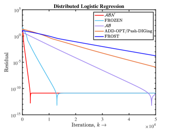
Figure 1: Strongly-convex case: Accelerated linear rate

IV-B Non strongly-convex case

We next choose the objective functions, $f_{i}$’s, to be smooth, convex but not strongly-convex. In particular, $f_{i}(x)=u(x)+b_{i}x$, where $b_{i}$’s are randomly generated, $b_{n}=-\sum_{i=1}^{n-1}b_{i}$, and $u(x)$ is chosen as follows:

$$u(x)=\left\{\begin{array}[]{rl}\frac{1}{4}x^{4},&|x|\leq 1,\\ |x|-\frac{3}{4},&|x|>1.\end{array}\right.$$

It can be verified that $f=\sum_{i}f_{i}$ is not strongly-convex as $f^{{}^{\prime\prime}}(x^{*})=0$. The results are shown in Fig. 2 where the momentum parameter is chosen as $\beta_{k}=\frac{k}{k+3}$ and other parameters are manually optimized.

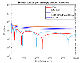
Figure 2: Non strongly-convex case: Accelerated sublinear rate

IV-C Influence of graph sparsity

Finally, we study the influence of graph sparsity with the help of the logistic regression problem discussed earlier. We fix the number of nodes to $n=30$ and randomly generate three nearest-neighbor digraphs, $\mathcal{G}_{1}$, $\mathcal{G}_{2}$ and $\mathcal{G}_{3}$, with decreasing sparsity, see Fig. 3 (Top). In Fig. 3 (Bottom), we compare the performance of the proposed methods with centralized Nesterov over the three graphs. It can be verified that $\mathcal{ABN}$ and FROZEN approach centralized Nesterov method as the graphs become dense. FROZEN, however, is much slower than $\mathcal{ABN}$ because it additionally requires eigenvector learning.

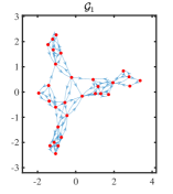
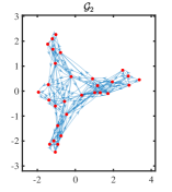
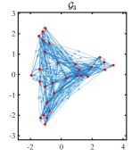
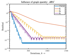
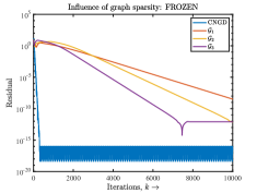
Figure 3: Influence of digraph sparsity on $\mathcal{ABN}$ and FROZEN.

V Conclusions

In this letter, we present accelerated methods for optimization based on Nesterov’s momentum over arbitrary, strongly-connected, graphs. The fundamental algorithm, $\mathcal{ABN}$, uses both row- and column-stochastic weights, simultaneously, to achieve agreement and optimality. We then derive a variant from $\mathcal{ABN}$, termed as FROZEN, that only uses row-stochastic weights and thus is applicable to a larger set of communication protocols, however, at the expense of eigenvector learning, thus resulting into slower convergence. Although a theoretical analysis is beyond the scope of this letter, we provide an extensive set of numerical results to study the behavior of the proposed methods for both convex and strongly-convex cases.

References

- [1] M. Rabbat and R. Nowak, “Distributed optimization in sensor networks,” in 3rd International Symposium on Information Processing in Sensor Networks, Berkeley, CA, Apr. 2004, pp. 20–27.
- [2] J. Chen and A. H. Sayed, “Diffusion adaptation strategies for distributed optimization and learning over networks,” IEEE Trans. on Signal Processing, vol. 60, no. 8, pp. 4289–4305, Aug. 2012.
- [3] A. Mokhtari, W. Shi, Q. Ling, and A. Ribeiro, “A decentralized second-order method with exact linear convergence rate for consensus optimization,” IEEE Trans. on Signal and Information Processing over Networks, vol. 2, no. 4, pp. 507–522, 2016.
- [4] S. Safavi, U. A. Khan, S. Kar, and J. M. F. Moura, “Distributed localization: A linear theory,” Proceedings of the IEEE, vol. 106, pp. 1204–1223, Jul. 2018.
- [5] P. A. Forero, A. Cano, and G. B. Giannakis, “Consensus-based distributed support vector machines,” Journal of Machine Learning Research, vol. 11, no. May, pp. 1663–1707, 2010.
- [6] S. Boyd, N. Parikh, E. Chu, B. Peleato, and J. Eckstein, “Distributed optimization and statistical learning via the alternating direction method of multipliers,” Foundation and Trends in Maching Learning, vol. 3, no. 1, pp. 1–122, Jan. 2011.
- [7] H.-T. Wai, Z. Yang, Z. Wang, and M. Hong, “Multi-agent reinforcement learning via double averaging primal-dual optimization,” arXiv preprint arXiv:1806.00877, 2018.
- [8] X. Lian, C. Zhang, H. Zhang, C. Hsieh, W. Zhang, and J. Liu, “Can decentralized algorithms outperform centralized algorithms? A case study for decentralized parallel stochastic gradient descent,” in Advances in Neural Information Processing Systems, 2017, pp. 5330–5340.
- [9] M. Hong, D. Hajinezhad, and M. Zhao, “Prox-PDA: The proximal primal-dual algorithm for fast distributed nonconvex optimization and learning over networks,” in International Conference on Machine Learning, 2017, pp. 1529–1538.
- [10] K. Scaman, F. Bach, S. Bubeck, L. Massoulié, and Y. T. Lee, “Optimal algorithms for non-smooth distributed optimization in networks,” in Advances in Neural Information Processing Systems, 2018, pp. 2745–2754.
- [11] S. S. Ram, A. Nedić, and V. V. Veeravalli, “Distributed subgradient projection algorithm for convex optimization,” in IEEE International Conference on Acoustics, Speech and Signal Processing, Taipei, Taiwan, Apr. 2009, pp. 3653–3656.
- [12] A. Nedić and A. Ozdaglar, “Distributed subgradient methods for multi-agent optimization,” IEEE Trans. on Automatic Control, vol. 54, no. 1, pp. 48–61, Jan. 2009.
- [13] K. Srivastava and A. Nedić, “Distributed asynchronous constrained stochastic optimization,” IEEE Journal of Selected Topics in Signal Processing, vol. 5, no. 4, pp. 772–790, 2011.
- [14] S. Lee and A. Nedić, “Distributed random projection algorithm for convex optimization,” IEEE Journal of Selected Topics in Signal Processing, vol. 7, no. 2, pp. 221–229, Apr. 2013.
- [15] S. Safavi and U. A. Khan, “Revisiting finite-time distributed algorithms via successive nulling of eigenvalues,” IEEE Signal Processing Letters, vol. 22, no. 1, pp. 54–57, Jan. 2015.
- [16] R. Olfati-Saber and R. M. Murray, “Consensus problems in networks of agents with switching topology and time-delays,” IEEE Trans. on Automatic Control, vol. 49, no. 9, pp. 1520–1533, Sep. 2004.
- [17] Lin Xiao and Stephen Boyd, “Fast linear iterations for distributed averaging,” Systems & Control Letters, vol. 53, no. 1, pp. 65–78, 2004.
- [18] J. Xu, S. Zhu, Y. C. Soh, and L. Xie, “Augmented distributed gradient methods for multi-agent optimization under uncoordinated constant stepsizes,” in IEEE 54th Annual Conference on Decision and Control, 2015, pp. 2055–2060.
- [19] G. Qu and N. Li, “Harnessing smoothness to accelerate distributed optimization,” IEEE Trans. on Control of Network Systems, Apr. 2017.
- [20] W. Shi, Q. Ling, G. Wu, and W Yin, “Extra: An exact first-order algorithm for decentralized consensus optimization,” SIAM Journal on Optimization, vol. 25, no. 2, pp. 944–966, 2015.
- [21] K. I. Tsianos, The role of the Network in Distributed Optimization Algorithms: Convergence Rates, Scalability, Communication/Computation Tradeoffs and Communication Delays, Ph.D. thesis, Dept. Elect. Comp. Eng. McGill University, 2013.
- [22] A. Nedić and A. Olshevsky, “Distributed optimization over time-varying directed graphs,” IEEE Trans. on Automatic Control, vol. 60, no. 3, pp. 601–615, Mar. 2015.
- [23] C. Xi and U. A. Khan, “Distributed subgradient projection algorithm over directed graphs,” IEEE Trans. on Automatic Control, vol. 62, no. 8, pp. 3986–3992, Oct. 2016.
- [24] C. Xi, Q. Wu, and U. A. Khan, “On the distributed optimization over directed networks,” Neurocomputing, vol. 267, pp. 508–515, Dec. 2017.
- [25] C. Xi, R. Xin, and U. A. Khan, “ADD-OPT: Accelerated distributed directed optimization,” IEEE Trans. on Automatic Control, Aug. 2017, in press.
- [26] A. Nedić, A. Olshevsky, and W. Shi, “Achieving geometric convergence for distributed optimization over time-varying graphs,” SIAM Journal of Optimization, Dec. 2017.
- [27] C. Xi, V. S. Mai, R. Xin, E. Abed, and U. A. Khan, “Linear convergence in optimization over directed graphs with row-stochastic matrices,” IEEE Trans. on Automatic Control, Jan. 2018, in press.
- [28] R. Xin, C. Xi, and U. A. Khan, “FROST – Fast row-stochastic optimization with uncoordinated step-sizes,” Arxiv: https://arxiv.org/abs/1803.09169, Mar. 2018.
- [29] D. Kempe, A. Dobra, and J. Gehrke, “Gossip-based computation of aggregate information,” in 44th Annual IEEE Symposium on Foundations of Computer Science, Oct. 2003, pp. 482–491.
- [30] F. Benezit, V. Blondel, P. Thiran, J. Tsitsiklis, and M. Vetterli, “Weighted gossip: Distributed averaging using non-doubly stochastic matrices,” in IEEE International Symposium on Information Theory, Jun. 2010, pp. 1753–1757.
- [31] K. Cai and H. Ishii, “Average consensus on general strongly connected digraphs,” Automatica, vol. 48, no. 11, pp. 2750 – 2761, 2012.
- [32] R. Xin and U. A. Khan, “Distributed heavy-ball: A generalization and acceleration of first-order methods with gradient tracking,” arXiv preprint arXiv:1808.02942, 2018.
- [33] R. Xin and U. A. Khan, “A linear algorithm for optimization over directed graphs with geometric convergence,” IEEE Control Systems Letters, vol. 2, no. 3, pp. 325–330, Jul. 2018.
- [34] B. Polyak, Introduction to optimization, Optimization Software, 1987.
- [35] Y. Nesterov, Introductory lectures on convex optimization: A basic course, vol. 87, Springer Science & Business Media, 2013.
- [36] F. Saadatniaki, R. Xin, and U. A. Khan, “Optimization over time-varying directed graphs with row and column-stochastic matrices,” arXiv preprint arXiv:1810.07393, 2018.
- [37] S. Pu, W. Shi, J. Xu, and A. Nedić, “Push-pull gradient methods for distributed optimization in networks,” arXiv preprint arXiv:1803.07588, 2018.
- [38] A. Daneshmand, G. Scutari, and V. Kungurtsev, “Second-order guarantees of distributed gradient algorithms,” arXiv preprint arXiv:1809.08694, 2018.
- [39] D. Jakovetic, J. Xavier, and J. M. F. Moura, “Fast distributed gradient methods,” IEEE Trans. on Automatic Control, vol. 59, no. 5, pp. 1131–1146, 2014.
- [40] D. Jakovetic, J. M. F. Xavier, and José M. F. Moura, “Convergence rates of distributed nesterov-like gradient methods on random networks.,” IEEE Trans. Signal Processing, vol. 62, no. 4, pp. 868–882, 2014.
- [41] G. Qu and N. Li, “Accelerated distributed Nesterov gradient descent,” Arxiv: https://arxiv.org/abs/1705.07176, May 2017.
- [42] T. Wu, K. Yuan, Q. Ling, W. Yin, and A. H. Sayed, “Decentralized consensus optimization with asynchrony and delays,” IEEE Transactions on Signal and Information Processing over Networks, vol. 4, no. 2, pp. 293–307, 2018.
- [43] Y. Tian, Y. Sun, B. Du, and G. Scutari, “Asy-sonata: Achieving geometric convergence for distributed asynchronous optimization,” arXiv preprint arXiv:1803.10359, 2018.