Learning Graph Pooling and Hybrid Convolutional Operations for Text Representations

Abstract.

With the development of graph convolutional networks (GCN), deep learning methods have started to be used on graph data. In additional to convolutional layers, pooling layers are another important components of deep learning. However, no effective pooling methods have been developed for graphs currently. In this work, we propose the graph pooling (gPool) layer, which employs a trainable projection vector to measure the importance of nodes in graphs. By selecting the $k$-most important nodes to form the new graph, gPool achieves the same objective as regular max pooling layers operation on images and texts. Another limitation of GCN when used on graph-based text representation tasks is that, GCNs do not consider the order information of nodes in graph. To address this limitation, we propose the hybrid convolutional (hConv) layer that combines GCN and regular convolutional operations. The hConv layer is capable of increasing receptive fields quickly and computing features automatically. Based on the proposed gPool and hConv layers, we develop new deep networks for text categorization tasks. Our experimental results show that the networks based on gPool and hConv layers achieves new state-of-the-art performance as compared to baseline methods.

1. Introduction

Convolutional neural networks (CNNs) (LeCun et al., 1998) have shown great capability of solving challenging tasks in various fields such as computer vision and natural language processing (NLP). A variety of CNN networks have been proposed to continuously set new performance records (Krizhevsky et al., 2012; Simonyan and Zisserman, 2015; He et al., 2016; Huang et al., 2017). In addition to image-related tasks, CNNs are also successfully applied to NLP tasks such as text classification (Zhang et al., 2015) and neural machine translation (Bahdanau et al., 2015; Vaswani et al., 2017). The power of CNNs lies in trainable local filters for automatic feature extraction. The networks can decide which kind of features to extract with the help of these trainable local filters, thereby avoiding hand-crafted feature extractors (Wang et al., 2012).

One common characteristic behind the above tasks is that both images and texts can be represented in grid-like structures, thereby enabling the application of convolutional operations. However, some data in real-world can be naturally represented as graphs such as social networks. There are primarily two types of tasks on graph data; those are, node classification (Kipf and Welling, 2017; Veličković et al., 2017) and graph classification (Niepert et al., 2016; Wu et al., 2017). Graph convolutional networks (GCNs) (Kipf and Welling, 2017) and graph attention networks (GATs) (Veličković et al., 2017) have been proposed for node classification tasks under both transductive and inductive learning settings. However, GCNs lack the capability of automatic high-level feature extraction, since no trainable local filters are used.

In addition to convolutional layers, pooling layers are another important components in CNNs by helping to enlarge receptive fields and reduce the risk of over-fitting. However, there are still no effective pooling operations that can operate on graph data and extract sub-graphs. Meanwhile, GCNs have been applied on text data by converting texts into graphs (Schlichtkrull et al., 2017; Liu et al., 2018). Although GCNs can operate on graphs converted from texts, they ignore the ordering information between nodes, which correspond to words in texts.

In this work, we propose a novel pooling layer, known as the graph pooling (gPool) layer, that acts on graph data. Our method employs a trainable projection vector to measure the importance of nodes in a graph. Based on measurement scores, we rank and select $k$-largest nodes to form a new sub-graph, thereby achieving pooling operation on graph data. When working on graphs converted from text data, the words are treated as nodes in the graphs. By maintaining the order information in nodes’ feature matrices, we can apply convolutional operations to feature matrices. Based on this observation, we develop a new graph convolutional layer, known as the hybrid convolutional (hConv) layer. Based on gPool and hConv layers, we develop a shallow but effective architecture for text modeling tasks (Long et al., 2015). Results on text classification tasks demonstrate the effectiveness of our proposed methods as compared to previous CNN models.

2. Related Work

Before applying graph-based methods on text data, we need to convert texts to graphs. In this section, we discuss related literatures on converting texts to graphs and use of GCNs on text data.

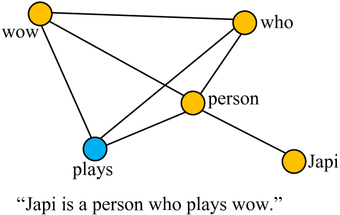
Figure 1. Example of converting text to a graph using the graph-of-words method. For this text, we use noun, adjective, and verb as terms for node selection. The words of “Japi”, “person”, “who”, “plays”, and “wow” are selected as nodes in the graph. We employ a sliding window size of 4 for edge building. For instance, there is an undirected edge between “Japi” and “person”, since they can be covered in the same sliding window in the original text.

2.1. Text to Graph Conversion

Many graph representations of texts have been explored to capture the inherent topology and dependence information between words. Bronselaer and Pasi (2013) employed a rule-based classifier to map each tag onto graph nodes and edges. The tags are acquired by the part-of-speech (POS) tagging techniques. In (Liu et al., 2018) a concept interaction graph representation is proposed for capturing complex interactions among sentences and concepts in documents. The graph-of-word representation (GoW) (Mihalcea and Tarau, 2004) attempts to capture co-occurrence relationships between words known as terms. It was initially applied to text ranking task and has been widely used in many NLP tasks such as information retrieval (Rousseau and Vazirgiannis, 2013), text classification (Rousseau et al., 2015; Malliaros and Skianis, 2015), keyword extraction (Rousseau and Vazirgiannis, 2015; Tixier et al., 2016) and document similarity measurement (Nikolentzos et al., 2017).

Before applying graph-based text modeling methods, we need to convert texts to graphs. In this work, we employ the graph-of-words (Mihalcea and Tarau, 2004) method for its effectiveness and simplicity. The conversion starts with the phase preprocessing such as tokenization and text cleaning. After preprocessing, each text is encoded into an unweighted and undirected graph in which nodes represent selected terms and edges represent co-occurrences between terms within a fixed sliding window. A term is a group of words clustered based on their part-of-speech tags such as noun and adjective. The choice of sliding window size depends on the average lengths of processed texts. Figure 1 provides an example of this method.

2.2. GCN and its Applications on Text Modeling

Recently, many studies (Kipf and Welling, 2017; Veličković et al., 2017) have attempted to apply convolutional operations on graph data. Graph convolutional networks (GCNs) (Kipf and Welling, 2017) were proposed and have achieved the state-of-the-art performance on inductive and transductive node classification tasks. The spectral graph convolution operation is defined such that a convolution-like operation can be applied on graph data. Basically, each GCN layer updates the feature representation of each node by aggregating the features of its neighboring nodes. To be specific, the layer-wise propagation rule of GCNs can be defined as $\mbox{gcn}(\hat{A},X_{\ell})=\sigma(\hat{D}^{-\frac{1}{2}}\hat{A}\hat{D}^{-\frac{1}{2}}X_{\ell}W_{\ell})$, where $X_{\ell}$ and $X_{\ell+1}$ are input and output matrices of layer $\ell$, respectively. The numbers of rows of two matrices are the same, which indicates that the number of nodes in graph does not change in GCN layers. We use $\hat{A}=A+I$ to include self-loop edges to the graph. The diagonal node degree matrix $\hat{D}$ is generated to normalize $\hat{A}$ such that the scale of feature vectors remains the same after aggregation. $W^{\ell}$ is the trainable weight matrix, which plays the role of linear transformation of each node’s feature vector. Finally, $\sigma(\cdot)$ denotes the nonlinear activation function such as ReLU (Nair and Hinton, 2010). Later, graph attention networks (GAT) (Veličković et al., 2017) are proposed to solve node classification tasks by using the attention mechanism (Xu et al., 2015).

In addition to graph data, some studies attempted to apply graph-based methods to grid-like data such as texts. Compared to traditional recurrent neural networks such as LSTM (Hochreiter and Schmidhuber, 1997), GCNs have the advantage of considering long-term dependencies by edges in graphs. Marcheggiani and Titov (2017) applied a variant of GCNs to the task of sentence encoding and achieved better performance than LSTM. GCNs have also been used in neural machine translation tasks (Bastings et al., 2017). Although graph convolutional operations have been extensively developed and explored, pooling operations on graphs are not well studied currently.

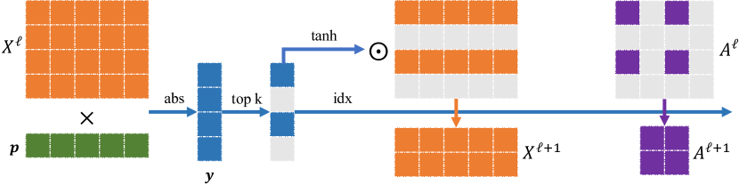
Figure 2. An illustration of the proposed graph pooling layer which samples $k=2$ nodes. $\times$ and $\odot$ represent matrix and element-wise multiplication, respectively. This example graph has four nodes, each of which contains 5 features. We have the adjacency matrix $A^{\ell}\in\mathbb{R}^{4\times 4}$ and the input feature matrix $X^{\ell}\in\mathbb{R}^{4\times 5}$ of layer $\ell$ representing this graph. $\mathbf{p}\in\mathbb{R}^{5}$ is a trainable projection vector in this layer. By matrix multiplication and $\mbox{abs}(\cdot)$, we have scores $\mathbf{y}$ which estimate the closeness of each node to the projection vector. Using $k=2$, we select two nodes with the highest scores and record their indices in idx, which represents indices of selected nodes. With indices idx, we extract corresponding nodes to form the new graph, which results in a new pooled feature map $\tilde{X}^{\ell}$ and adjacency matrix $A^{\ell+1}$. To control information flow, we create a gate vector by applying element-wise $\tanh(\cdot)$ to score vector $\mathbf{y}$. By element-wise multiplication between gate vector and $\tilde{X}^{\ell}$, we obtain the $X^{\ell+1}$. Outputs of this graph pooling layer are $A^{\ell+1}$ and $X^{\ell+1}$.

3. Graph Pooling and Hybrid Convolutional Operations

In this section, we describe our proposed graph pooling (gPool) and hybrid convolutional (hConv) operations. Based on these two new layers, we develop FCN-like graph convolutional networks for text modeling tasks.

3.1. Graph Pooling Layer

Pooling layers are very important for CNNs on grid-like data such as images, as they can help quickly enlarge receptive fields and reduce feature map size, thereby resulting in better generalization and performance (Yu and Koltun, 2016). In pooling layers, input feature maps are partitioned into a set of non-overlapping rectangles on which non-linear down-sampling functions, such as maximum, are applied. Obviously, the partition scheme depends on the local adjacency on grid-like data like images. For instance in a max-pooling layer with a kernel size of $2\times 2$, 4 spatially adjacent units form a partition. However, such kind of spatial adjacency information is not available for nodes on graphs. We cannot directly apply regular pooling layers to graph data.

To enable pooling operations on graph data, we propose the graph pooling layer (gPool), which adaptively selects a subset of important nodes to form a smaller new graph. Suppose a graph has $N$ nodes and each node contains $C$ features. We can represent the graph with two matrices; those are the adjacency matrix $A^{\ell}\in\mathbb{R}^{N\times N}$ and the feature matrix $X^{\ell}\in\mathbb{R}^{N\times C}$. Each row in $X^{\ell}$ corresponds to a node in the graph. We propose the layer-wise propagation rule of gPool to be defined as

(1) $$\mathbf{y} =|X^{\ell}\mathbf{p}^{\ell}|, =\mbox{rank}(\mathbf{y},k),$$ idx

$$A^{\ell+1} =A^{\ell}(\mbox{idx},\mbox{idx}), \tilde{X}^{\ell} =X^{\ell}(\mbox{idx},\mathrel{\mathop{\mathchar 58\relax}}),$$

$$\tilde{\mathbf{y}} =\tanh(\mathbf{y}(\mbox{idx})), X^{\ell+1} =\tilde{X}^{\ell}\odot\left(\tilde{\mathbf{y}}\mathbf{1}_{C}^{T}\right),$$

where $k$ is the number of nodes to be selected from the graph, $\mathbf{p}^{\ell}\in\mathbb{R}^{C}$ is a trainable projection vector of layer $\ell$, $\mbox{rank}(\mathbf{y})$ is an operation that returns the indices corresponding to the $k$-largest values in $\mathbf{y}$, $A^{\ell}(\mbox{idx},\mbox{idx})$ extracts the rows and columns with indices idx, $X^{\ell}(\mbox{idx},\mathrel{\mathop{\mathchar 58\relax}})$ selects the rows with indices idx using all column values, $\mathbf{y}(\mbox{idx})$ returns the corresponding values in $\mathbf{y}$ with indices idx, $\mathbf{1}_{C}\in\mathbb{R}^{C}$ is a vector of size $C$ with all components being 1, and $\odot$ denotes the element-wise matrix multiplication operation.

Suppose $X^{\ell}$ is a matrix with row vectors $\mathbf{x}^{\ell}_{1},\mathbf{x}^{\ell}_{2},\cdots,\mathbf{x}^{\ell}_{N}$. We first perform a matrix multiplication between $X^{\ell}$ and $\mathbf{p}^{\ell}$ followed by an element-wise $\mbox{abs}(\cdot)$ operation, resulting in $\mathbf{y}=[y_{1},y_{2},\cdots,y_{N}]^{T}$ with each $y_{i}$ measuring the closeness between the node feature vector $\mathbf{x}^{\ell}_{i}$ and the projection vector $\mathbf{p}^{\ell}$.

The $\mbox{rank}(\cdot)$ operation ranks the $N$ values in $\mathbf{y}$ and returns the indices of the $k$-largest values. Suppose the indices of the $k$ selected values are $i_{1},i_{2},\cdots,i_{k}$ with $i_{m}<i_{n}$ if $1\leq m<n\leq k$. These indices correspond to nodes in the graph. Note that the selection process retains the order information of selected nodes in the original feature matrix. With indices, the $k$-node selection is conducted on the feature matrix $X^{l}$, the adjacency matrix $A^{\ell}$, and the score vector $\mathbf{y}$. We concatenate the corresponding feature vectors $\mathbf{x}^{\ell}_{i_{1}},\mathbf{x}^{\ell}_{i_{2}},\cdots,\mathbf{x}^{\ell}_{i_{k}}$ and output a matrix $\tilde{X}^{\ell}\in\mathbb{R}^{k\times C}$. Similarly, we use scores $\tanh(y_{i_{1}}),\tanh(y_{i_{2}}),\cdots,\tanh(y_{i_{k}})$ as elements of the vector $\mathbf{\tilde{y}}\in\mathbb{R}^{k}$. For the adjacency matrix $A^{\ell}$, we extract rows and columns based on the selected indices and output the adjacency matrix $A^{{\ell}+1}\in\mathbb{R}^{k\times k}$ for the new graph.

Finally, we perform a gate operation to control the information flow in this layer. Using element-wise product of $\tilde{X}^{\ell}$ and $\mathbf{\tilde{y}}\mathbf{1}^{T}_{C}$, features of selected nodes are filtered through their corresponding scores and form the output $X^{{\ell}+1}\in\mathbb{R}^{k\times C}$. The $i$th row vector in $X^{{\ell}+1}$ is the product of the corresponding row vector in $\tilde{X}^{\ell}$ and the $i^{th}$ scalar number in $\mathbf{\tilde{y}}$. In addition to information control, the gate operation also makes the projection vector $\mathbf{p}^{\ell}$ trainable with back-propagation (LeCun et al., 2012). Without the gate operation, the projection vector $\mathbf{p}^{\ell}$ only contributes discrete indices to outputs and thus is not trainable. Figure 2 provides an illustration of the gPool layer.

Compared to regular pooling layers used on grid-like data, our gPool layer involves extra parameters in the trainable projection vector $\mathbf{p}^{\ell}$. In Section 4.6, we show that the number of extra parameters is negligible and would not increase the risk of over-fitting.

3.2. Hybrid Convolutional Layer

It follows from the analysis in Section 2.2 that GCN layers only perform convolutional operations on each node. There is no trainable spatial filters as in regular convolution layers. GCNs do not have the power of automatic feature extraction as achieved by CNNs. This limits the capability of GCNs, especially in the field of graph modeling. In traditional graph data, there is no ordering information among nodes. In addition, the different numbers of neighbors for each node in the graph prohibit convolutional operations with a kernel size larger than 1. Although we attempt to modeling texts as graph data, they are essentially grid-like data with order information among nodes, thereby enabling the application of regular convolutional operations.

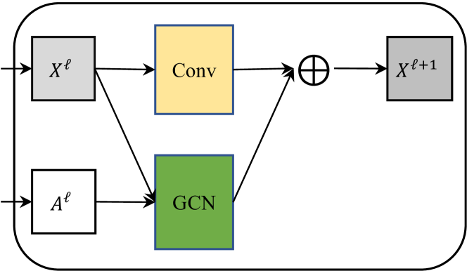
Figure 3. An illustration of the hybrid convolutional layer. $\oplus$ denotes matrix concatenation along the row dimension. In this layer, $A^{\ell}$ and $X^{\ell}$ are the adjacency matrix and the node feature matrix, respectively. A regular 1-D convolutional operation is used to extract high-level features from sentence texts. The GCN operation is applied at the graph level for feature extraction. The two intermediate outputs are concatenated together to form the final output $X^{\ell+1}$.

To take advantage of convolutional operations with trainable filters, we propose the hybrid convolutional layer (hConv), which combines GCN operations and regular 1-D convolutional operations to achieve the capability of automatic feature extraction. Formally, we propose the hConv layer to be defined as

(2) $$X^{\ell+1}_{1} =\mbox{conv}(X^{\ell}), X^{\ell+1}_{2} =\mbox{gcn}(A^{\ell},X^{\ell}),$$

$$X^{\ell+1} =\big{[}X^{\ell+1}_{1},X^{\ell+1}_{2}\big{]},$$

where $\mbox{conv}(\cdot)$ denotes a regular 1-D convolutional operation, and the $\mbox{gcn}(\cdot,\cdot)$ operation is defined in Eq. LABEL:eq:gcn. For the feature matrix $X^{\ell}$, we treat the column dimension as the channel dimension, such that the 1-D convolutional operation can be applied along the row dimension. Using the 1-D convolutional operation and the GCN operation, we obtain two intermediate outputs; those are $X^{\ell+1}_{1}$ and $X^{\ell+1}_{2}$. These two matrices are concatenated together as the layer output $X^{\ell+1}$. Figure 3 illustrates an example of the hConv layer.

We argue that the integration of GCN operations and 1-D convolutional operations in the hConv layer is especially applicable to graph data obtained from texts. By representing texts as an adjacency matrix $A^{\ell}$ and a node feature matrix $X^{\ell}$ of layer $\ell$, each node in the graph is essentially a word in the text. We retain the order information of nodes from their original relative positions in texts. This indicates that the feature matrix $X^{\ell}$ is organized as traditional grid-like data with order information retained. From this point, we can apply an 1-D convolutional operation with kernel sizes larger than 1 on the feature matrix $X^{\ell}$ for high-level feature extraction.

The combination of the GCN operation and the convolutional operation in the hConv layer can take the advantages of both of them and overcome their respective limitations. In convolutional layers, the receptive fields of units on feature maps increase very slow since small kernel sizes are usually used to avoid massive number of parameters. In contrast, GCN operations can help to increase the receptive fields quickly by means of edges between terms in sentences corresponding to nodes in graphs. At the same time, GCN operations are not able to automatically extract high-level features as they do not have trainable spatial filters as used in convolutional operations. From this point, the hConv layer is especially useful when working on text-based graph data such as sentences and documents.

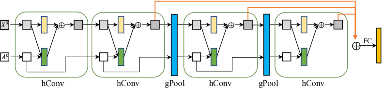
Figure 4. The architecture of the hConv-gPool-Net. $\oplus$ denotes the concatenation operation of feature maps. The inputs of the network are an adjacency matrix $A^{0}$ and a feature matrix $X^{0}$. We stack four hConv layers for feature extraction. In the second and the third hConv layers, we employ the gPool layers to reduce the number of nodes in graphs by half. Starting from the second hConv layer, a global max-pooling layer is applied to the output feature maps of each hConv layer. The outputs of these pooling layers are concatenated together. Finally, we employ a fully-connected layer for predictions. To obtain the other three networks discussed in Section 3.3, we can simply replace the hConv layers with GCN layers or remove gPool layers based on this network architecture.

3.3. Network Architectures

Based on our proposed gPool and hConv layers, we design four network architectures, including our baseline with a FCN-like (Long et al., 2015) architecture. FCN has been shown to be very effective for image semantic segmentation. It allows final linear classifiers to make use of features from different layers. Here, we design four architectures based on our proposed gPool and hConv layers.

• GCN-Net: We establish a baseline method by using GCN layers to build a network without any hConv or gPool layers. In this network, we stack 4 standard GCN layers as feature extractors. Starting from the second layer, a global max-pooling layer (Lin et al., 2013) is applied to each layer’s output. The outputs of these pooling layers are concatenated together and fed into a fully-connected layer for final predictions. This network serves as a baseline model in this work for experimental studies.

• GCN-gPool-Net: In this network, we add our proposed gPool layers to GCN-Net. Starting from the second layer, we add a gPool layer after each GCN layer except for the last one. In each gPool layer, we select the hyper-parameter $k$ to reduce the number of nodes in the graph by a factor of two. All other parts of the network remain the same as those of GCN-Net.

• hConv-Net: For this network, we replace all GCN layers in GCN-Net by our proposed hConv layers. To ensure the fairness of comparison among these networks, the hConv layers output the same number of feature maps as the corresponding GCN layers. Suppose the original $i$th GCN layer outputs $n_{out}$ feature maps. In the corresponding hConv layer, both the GCN operation and the convolutional operation output $n_{out}/2$ feature maps. By concatenating those intermediate outputs, the $i$th hConv layer also outputs $n_{out}$ feature maps. The remaining parts of the network remain the same as those in GCN-Net.

• hConv-gPool-Net: Based on the hConv-Net network, we add gPool layers after each hConv layer except for the first and the last layers. We employ the same principle for the selection of hyper-parameter $k$ as that in GCN-gPool-Net. The remaining parts of the network remain the same. Note that gPool layers maintain the order information of nodes in the new graph, thus enabling the application of 1-D convolutional operations in hConv layers afterwards. Figure 4 provides an illustration of the hConv-gPool-Net network.

Datasets	#Training	#Testing	#Classes	#Words
AG’s News	120,000	7,600	4	45
DBPedia	560,000	70,000	14	55
Yelp Polarity	560,000	38,000	2	153
Yelp Full	650,000	50,000	5	155

Table 1. Summary of datasets used in our experiments. The #words denotes the average number of words of the data samples for each dataset. These numbers help the selection of the sliding window size used in converting texts to graphs.

Models	AG’s News	DBPedia	Yelp Polarity	Yelp Full
Word-level CNN (Zhang et al., 2015)	8.55%	1.37%	4.60%	39.58%
Char-level CNN (Zhang et al., 2015)	9.51%	1.55%	4.88%	37.95%
GCN-Net	8.64%	1.69%	7.74%	42.60%
GCN-gPool-Net	8.09%	1.44%	5.82%	41.83%
hConv-Net	7.49%	1.02%	4.45%	37.81%
hConv-gPool-Net	7.09%	0.92%	4.37%	36.27%

Table 2. Results of text classification experiments in terms of classification error rate on the AG’s News, DBPedia, Yelp Review Polarity, and Yelp Review Full datasets. The first two methods are the state-of-the-art models without using any unsupervised data. The last four networks are proposed in this work.

4. Experimental Study

In this section, we evaluate our gPool layer and hConv layer based on the four networks proposed in Section 3.3. We compare the performances of our networks with that of previous state-of-the-art models. The experimental results show that our methods yield improved performance in terms of classification accuracy. We also perform some ablation studies to examine the contributions of the gPool layer and the hConv layer to the performance. The number of extra parameters in gPool layers is shown to be negligible and will not increase the risk of over-fitting.

4.1. Datasets

In this work, we evaluate our methods on four datasets, including the AG’s News, Dbpedia, Yelp Polarity, and Yelp Full (Zhang et al., 2015) datasets.

AG’s News is a news dataset containing four topics: World, Sports, Business and Sci/Tech. The task is to classify each news into one of the topics.

Dbpedia ontology dataset contains 14 ontology classes. It is constructed by choosing 14 non-overlapping classes from the DBPedia 2014 dataset (Lehmann et al., 2015). Each sample contains a title and an abstract corresponding to a Wikipedia article.

Yelp Polarity dataset is obtained from the Yelp Dataset Challenge in 2015 (Zhang et al., 2015). Each sample is a piece of review text with a binary label (negative or positive).

Yelp Full dataset is obtained from the Yelp Dataset Challenge in 2015, which is for sentiment classification (Zhang et al., 2015). It contains five classes corresponding to the movie review star ranging from 1 to 5.

The summary of these datasets are provided in Table 1. For all datasets, we tokenize the textual document and convert words to lower case. We remove stop-words and all punctuation in texts. Based on cleaned texts, we build the graph-of-word representations for texts.

4.2. Text to Graph Conversion

We use the graph-of-words method to convert texts into graph representations that include an adjacency matrix and a feature matrix. We select nouns, adjective, and verb as terms, meaning a word appears in the graph if it belongs to one of the above categories. We use a sliding window to decide if two terms have an edge between them. If the distance between two terms is less than the window size, an undirected edge between these two terms is added. In the generated graph, nodes are the terms appear in texts, and edges are added using the sliding window. We use a window size of 4 for the AG’s News and DBpedia datasets and 10 for the other two datasets, depending on their average words in training samples. The maximum numbers of nodes in graphs for the AG’s News, DBPedia, Yelp Polarity, Yelp Full datasets are 100, 100, 300, and 256, respectively.

To produce the feature matrix, we use word embedding and position embedding features. For word embedding features, the pre-trained fastText word embedding vectors (Joulin et al., 2017) are used, and it contains more than 2 million pre-trained words vectors. Compared to other pre-trained word embedding vectors such as GloVe (Pennington et al., 2014), using the fastText helps us to avoid massive unknown words. On the AG’s News dataset, the number of unknown words with the fastText is only several hundred, which is significantly smaller than the number using GloVe. In addition to word embedding features, we also employ position embedding method proposed in Zeng et al. (2014). We encode the positions of words in texts into one-hot vectors and concatenate them with word embedding vectors. We obtain the feature matrix by stacking word vectors of nodes in the row dimension.

Models	Depth	Error Rate
Word-level CNN	9	8.55%
Character-level CNN	9	9.51%
GCN-Net	5	8.64%
GCN-gPool-Net	5	8.09%
hConv-Net	5	7.49%
hConv-gPool-Net	5	7.09%

Table 3. Comparison in terms of the network depth and the text classification error rate on the AG’s News dataset. The depth listed here is calculated by counting the number of convolutional and fully-connected layers in networks.

4.3. Experimental Setup

For our proposed networks, we employ the same settings with minor adjustments to accommodate the different datasets. As discussed in Section 3.3, we stack four GCN or hConv layers for GCN-based networks or hConv-based networks. For the networks using gPool layers, we add gPool layers after the second and the third GCN or hConv layers. Four GCN or hConv layers output 1024, 1024, 512, and 256 feature maps, respectively. We use this decreasing number of feature maps, since GCNs help to enlarge the receptive fields very quickly. We do not need more high-level features in deeper layers. The kernel sizes used by convolutional operations in hConv layers are all $3\times 1$. For all layers, we use the ReLU (Nair and Hinton, 2010) for nonlinearity. For all experiments, the following settings are shared. For training, the Adam optimizer (Kingma and Ba, 2015) is used for 60 epochs. The learning rate starts at 0.001 and decays by 0.1 at the 30${}^{t}h$ and the 50${}^{t}h$ epoch. We employ the dropout with a keep rate of 0.55 (Srivastava et al., 2014) and batch size of 256. These hyper-parameters are tuned on the AG’s News dataset, and then ported to other datasets.

4.4. Performance Study

We compare our proposed methods with other state-of-the-art models, and the experimental results are summarized in Table 2. We can see from the results that our hConv-gPool-Net outperforms both word-level CNN and character-level CNN by at least a margin of 1.46%, 0.45%, 0.23%, and 3.31% on the AG’s News, DBPedia, Yelp Polarity, and Yelp Full datasets, respectively. The performance of GCN-Net with only GCN layers cannot compete with that of word-level CNN and char-level CNN primarily due to the lack of automatic high-level feature extraction. By replacing GCN layers using our proposed hConv layers, hConv-Net achieves better performance than the two CNN models across four datasets. This demonstrates the promising performance of our hConv layer by employing regular convolutional operations for automatic feature extraction. By comparing the GCN-Net with GCN-gPool-Net, and hConv-Net with hConv-gPool-Net, we observe that our proposed gPool layers promote both models’ performance by at least a margin of 0.4%, 0.1%, 0.08%, and 1.54% on the AG’s News, DBPedia, Yelp Polarity, and Yelp Full datasets. The margins tend to be larger on harder tasks. This observation demonstrates that our gPool layer helps to enlarge receptive fields and reduce spatial dimensions of graphs, resulting in better generalization and performance.

Models	Error rate	# Params	Ratio of increase
GCN-Net	8.64%	1,554,820	0.00%
GCN-gPool-Net	8.09%	1,555,719	0.06%

Table 4. Comparison between the GCN-Net and GCN-gPool-Net in term of parameter numbers and text classification error rates on the AG’s News dataset.

4.5. Network Depth Study

In addition to performance study, we also conduct experiments to evaluate the relationship between performance and network depth in terms of the number of convolutional and fully-connected layers in models. The results are summarized in Table 3. We can observe from the results that our models only require 5 layers, including 4 convolutional layers and 1 fully-connected layer. Both word-level CNN and character-level CNN models need 9 layers in their networks, which are much deeper than ours. Our hConv-gPool-Net achieves the new state-of-the-art performance with fewer layers, demonstrating the effectiveness of gPool and hConv layers. Since GCN and gPool layers enlarge receptive fields quickly, advanced features are learned in shallow layers, leading to shallow networks but better performance.

4.6. Parameter Study of gPool Layer

Since gPool layers involve extra trainable parameters in projection vectors, we study the number of parameters in gPool layers in the GCN-gPool-Net that contains two gPool layers. The results are summarized in Table 4. We can see from the results that gPool layers only needs 0.06% additional parameters compared to GCN-Net. We believe that this negligible increase of parameters will not increase the risk of over-fitting. With negligible additional parameters, gPool layers can yield a performance improvement of 0.54%.

5. Conclusion

In this work, we propose the gPool and hConv layers in FCN-like graph convolutional networks for text modeling. The gPool layer achieves the effect of regular pooling operations on graph data to extract important nodes in graphs. By learning a projection vector, all nodes are measured through cosine similarity with the projection vector. The nodes with the $k$-largest scores are extracted to form a new graph. The scores are then applied to the feature matrix for information control, leading to the additional benefit of making the projection vector trainable. Since graphs are extracted from texts, we maintain the node orders as in the original texts. We propose the hConv layer that combines GCN and regular convolutional operations to enable automatic high-level feature extraction. Based on our gPool and hConv layers, we propose four networks for the task of text categorization. Our results show that the model based on gPool and hConv layers achieves new state-of-the-art performance compared to CNN-based models. gPool layers involve negligible number of parameters but bring significant performance boosts, demonstrating its contributions to model performance.

References

- (1)
- Bahdanau et al. (2015) Dzmitry Bahdanau, Kyunghyun Cho, and Yoshua Bengio. 2015. Neural machine translation by jointly learning to align and translate. International Conference on Learning Representations (2015).
- Bastings et al. (2017) Joost Bastings, Ivan Titov, Wilker Aziz, Diego Marcheggiani, and Khalil Sima’an. 2017. Graph convolutional encoders for syntax-aware neural machine translation. arXiv preprint arXiv:1704.04675 (2017).
- Bronselaer and Pasi (2013) Antoon Bronselaer and Gabriella Pasi. 2013. An approach to graph-based analysis of textual documents. In 8th European Society for Fuzzy Logic and Technology (EUSFLAT-2013). Atlantis Press, 634–641.
- He et al. (2016) Kaiming He, Xiangyu Zhang, Shaoqing Ren, and Jian Sun. 2016. Deep Residual Learning for Image Recognition. In Proceedings of the IEEE Conference on Computer Vision and Pattern Recognition.
- Hochreiter and Schmidhuber (1997) Sepp Hochreiter and Jürgen Schmidhuber. 1997. Long short-term memory. Neural computation 9, 8 (1997), 1735–1780.
- Huang et al. (2017) Gao Huang, Zhuang Liu, Kilian Q Weinberger, and Laurens van der Maaten. 2017. Densely connected convolutional networks. In Proceedings of the IEEE conference on computer vision and pattern recognition, Vol. 1. 3.
- Joulin et al. (2017) Armand Joulin, Edouard Grave, Piotr Bojanowski, and Tomas Mikolov. 2017. Bag of Tricks for Efficient Text Classification. In Proceedings of the 15th Conference of the European Chapter of the Association for Computational Linguistics: Volume 2, Short Papers, Vol. 2. 427–431.
- Kingma and Ba (2015) Diederik Kingma and Jimmy Ba. 2015. Adam: A method for stochastic optimization. The International Conference on Learning Representations (2015).
- Kipf and Welling (2017) Thomas N Kipf and Max Welling. 2017. Semi-supervised classification with graph convolutional networks. International Conference on Learning Representations (2017).
- Krizhevsky et al. (2012) Alex Krizhevsky, Ilya Sutskever, and Geoffrey E Hinton. 2012. Imagenet classification with deep convolutional neural networks. In Advances in neural information processing systems. 1097–1105.
- LeCun et al. (1998) Yann LeCun, Léon Bottou, Yoshua Bengio, and Patrick Haffner. 1998. Gradient-based learning applied to document recognition. Proc. IEEE 86, 11 (1998), 2278–2324.
- LeCun et al. (2012) Yann LeCun, Léon Bottou, Genevieve B Orr, and Klaus-Robert Müller. 2012. Efficient backprop. In Neural networks: Tricks of the trade. Springer, 9–48.
- Lehmann et al. (2015) Jens Lehmann, Robert Isele, Max Jakob, Anja Jentzsch, Dimitris Kontokostas, Pablo N Mendes, Sebastian Hellmann, Mohamed Morsey, Patrick Van Kleef, Sören Auer, et al. 2015. DBpedia–a large-scale, multilingual knowledge base extracted from Wikipedia. Semantic Web 6, 2 (2015), 167–195.
- Lin et al. (2013) Min Lin, Qiang Chen, and Shuicheng Yan. 2013. Network in network. arXiv preprint arXiv:1312.4400 (2013).
- Liu et al. (2018) Bang Liu, Ting Zhang, Di Niu, Jinghong Lin, Kunfeng Lai, and Yu Xu. 2018. Matching Long Text Documents via Graph Convolutional Networks. arXiv preprint arXiv:1802.07459 (2018).
- Long et al. (2015) Jonathan Long, Evan Shelhamer, and Trevor Darrell. 2015. Fully convolutional networks for semantic segmentation. In Proceedings of the IEEE conference on computer vision and pattern recognition. 3431–3440.
- Malliaros and Skianis (2015) Fragkiskos D Malliaros and Konstantinos Skianis. 2015. Graph-based term weighting for text categorization. In Advances in Social Networks Analysis and Mining (ASONAM), 2015 IEEE/ACM International Conference on. IEEE, 1473–1479.
- Marcheggiani and Titov (2017) Diego Marcheggiani and Ivan Titov. 2017. Encoding sentences with graph convolutional networks for semantic role labeling. arXiv preprint arXiv:1703.04826 (2017).
- Mihalcea and Tarau (2004) Rada Mihalcea and Paul Tarau. 2004. Textrank: Bringing order into text. In Proceedings of the 2004 conference on empirical methods in natural language processing.
- Nair and Hinton (2010) Vinod Nair and Geoffrey E Hinton. 2010. Rectified linear units improve restricted boltzmann machines. In Proceedings of the 27th international conference on machine learning (ICML-10). 807–814.
- Niepert et al. (2016) Mathias Niepert, Mohamed Ahmed, and Konstantin Kutzkov. 2016. Learning convolutional neural networks for graphs. In International Conference on Machine Learning. 2014–2023.
- Nikolentzos et al. (2017) Giannis Nikolentzos, Polykarpos Meladianos, François Rousseau, Yannis Stavrakas, and Michalis Vazirgiannis. 2017. Shortest-Path Graph Kernels for Document Similarity. In Proceedings of the 2017 Conference on Empirical Methods in Natural Language Processing. 1890–1900.
- Pennington et al. (2014) Jeffrey Pennington, Richard Socher, and Christopher Manning. 2014. Glove: Global vectors for word representation. In Proceedings of the 2014 conference on empirical methods in natural language processing (EMNLP). 1532–1543.
- Rousseau et al. (2015) François Rousseau, Emmanouil Kiagias, and Michalis Vazirgiannis. 2015. Text categorization as a graph classification problem. In Proceedings of the 53rd Annual Meeting of the Association for Computational Linguistics and the 7th International Joint Conference on Natural Language Processing (Volume 1: Long Papers), Vol. 1. 1702–1712.
- Rousseau and Vazirgiannis (2013) François Rousseau and Michalis Vazirgiannis. 2013. Graph-of-word and TW-IDF: new approach to ad hoc IR. In Proceedings of the 22nd ACM international conference on Information & Knowledge Management. ACM, 59–68.
- Rousseau and Vazirgiannis (2015) François Rousseau and Michalis Vazirgiannis. 2015. Main core retention on graph-of-words for single-document keyword extraction. In European Conference on Information Retrieval. Springer, 382–393.
- Schlichtkrull et al. (2017) Michael Schlichtkrull, Thomas N Kipf, Peter Bloem, Rianne van den Berg, Ivan Titov, and Max Welling. 2017. Modeling Relational Data with Graph Convolutional Networks. arXiv preprint arXiv:1703.06103 (2017).
- Simonyan and Zisserman (2015) Karen Simonyan and Andrew Zisserman. 2015. Very deep convolutional networks for large-scale image recognition. Proceedings of the International Conference on Learning Representations (2015).
- Srivastava et al. (2014) Nitish Srivastava, Geoffrey Hinton, Alex Krizhevsky, Ilya Sutskever, and Ruslan Salakhutdinov. 2014. Dropout: A simple way to prevent neural networks from overfitting. Journal of Machine Learning Research 15, 1 (2014), 1929–1958.
- Tixier et al. (2016) Antoine Tixier, Fragkiskos Malliaros, and Michalis Vazirgiannis. 2016. A graph degeneracy-based approach to keyword extraction. In Proceedings of the 2016 Conference on Empirical Methods in Natural Language Processing. 1860–1870.
- Vaswani et al. (2017) Ashish Vaswani, Noam Shazeer, Niki Parmar, Jakob Uszkoreit, Llion Jones, Aidan N Gomez, Łukasz Kaiser, and Illia Polosukhin. 2017. Attention is all you need. In Advances in Neural Information Processing Systems. 6000–6010.
- Veličković et al. (2017) Petar Veličković, Guillem Cucurull, Arantxa Casanova, Adriana Romero, Pietro Liò, and Yoshua Bengio. 2017. Graph Attention Networks. arXiv preprint arXiv:1710.10903 (2017).
- Wang et al. (2012) Tao Wang, David J Wu, Adam Coates, and Andrew Y Ng. 2012. End-to-end text recognition with convolutional neural networks. In Pattern Recognition (ICPR), 2012 21st International Conference on. IEEE, 3304–3308.
- Wu et al. (2017) Jia Wu, Shirui Pan, Xingquan Zhu, Chengqi Zhang, and S Yu Philip. 2017. Multiple structure-view learning for graph classification. IEEE transactions on neural networks and learning systems (2017).
- Xu et al. (2015) Kelvin Xu, Jimmy Ba, Ryan Kiros, Kyunghyun Cho, Aaron Courville, Ruslan Salakhudinov, Rich Zemel, and Yoshua Bengio. 2015. Show, attend and tell: Neural image caption generation with visual attention. In International conference on machine learning. 2048–2057.
- Yu and Koltun (2016) Fisher Yu and Vladlen Koltun. 2016. Multi-Scale Context Aggregation by Dilated Convolutions. In Proceedings of the International Conference on Learning Representations.
- Zeng et al. (2014) Daojian Zeng, Kang Liu, Siwei Lai, Guangyou Zhou, and Jun Zhao. 2014. Relation classification via convolutional deep neural network. In Proceedings of COLING 2014, the 25th International Conference on Computational Linguistics: Technical Papers. 2335–2344.
- Zhang et al. (2015) Xiang Zhang, Junbo Zhao, and Yann LeCun. 2015. Character-level convolutional networks for text classification. In Advances in neural information processing systems. 649–657.