Approximating the Perfect Sampling Grids for Computing the Eigenvalues of Toeplitz-like Matrices Using the Spectral Symbol

Sven-Erik Ekström
see@2pi.se
(Athens University of Economics and Business
)
Abstract

In a series of papers the author and others have studied an asymptotic expansion of the errors of the eigenvalue approximation, using the spectral symbol, in connection with Toeplitz (and Toeplitz-like) matrices, that is, Ej,nsubscript𝐸𝑗𝑛E_{j,n} in λj(An)=f(θj,n)+Ej,nsubscript𝜆𝑗subscript𝐴𝑛𝑓subscript𝜃𝑗𝑛subscript𝐸𝑗𝑛\lambda_{j}(A_{n})=f(\theta_{j,n})+E_{j,n}, An=Tn(f)subscript𝐴𝑛subscript𝑇𝑛𝑓A_{n}=T_{n}(f), f𝑓f real-valued cosine polynomial. In this paper we instead study an asymptotic expansion of the errors of the equispaced sampling grids θj,nsubscript𝜃𝑗𝑛\theta_{j,n}, compared to the exact grids ξj,nsubscript𝜉𝑗𝑛\xi_{j,n} (where λj(An)=f(ξj,n)subscript𝜆𝑗subscript𝐴𝑛𝑓subscript𝜉𝑗𝑛\lambda_{j}(A_{n})=f(\xi_{j,n})), that is, Ej,nsubscript𝐸𝑗𝑛E_{j,n} in ξj,n=θj,n+Ej,nsubscript𝜉𝑗𝑛subscript𝜃𝑗𝑛subscript𝐸𝑗𝑛\xi_{j,n}=\theta_{j,n}+E_{j,n}. We present an algorithm to approximate the expansion. Finally we show numerically that this type of expansion works for various kind of Toeplitz-like matrices (Toeplitz, preconditioned Toeplitz, low-rank corrections of them). We critically discuss several specific examples and we demonstrate the superior numerical behavior of the present approach with respect to the previous ones.

1 Introduction

For a given banded Hermitian Toeplitz matrix, Tn(f)n×nsubscript𝑇𝑛𝑓superscript𝑛𝑛T_{n}(f)\in\mathbb{R}^{n\times n},

Tn(f)=[f^0f^mf^mf^mf^mf^0]subscript𝑇𝑛𝑓delimited-[]subscript^𝑓0subscript^𝑓𝑚missing-subexpressionmissing-subexpressionmissing-subexpressionmissing-subexpressionmissing-subexpressionmissing-subexpressionmissing-subexpressionmissing-subexpressionmissing-subexpressionmissing-subexpressionmissing-subexpressionmissing-subexpressionsubscript^𝑓𝑚missing-subexpressionmissing-subexpressionmissing-subexpressionmissing-subexpressionmissing-subexpressionmissing-subexpressionmissing-subexpressionmissing-subexpressionmissing-subexpressionsubscript^𝑓𝑚missing-subexpressionmissing-subexpressionmissing-subexpressionmissing-subexpressionmissing-subexpressionmissing-subexpressionmissing-subexpressionmissing-subexpressionmissing-subexpressionmissing-subexpressionmissing-subexpressionmissing-subexpressionsubscript^𝑓𝑚subscript^𝑓0missing-subexpressionmissing-subexpressionmissing-subexpression\displaystyle T_{n}(f)=\left[\begin{array}[]{ccccccccc}\hat{f}_{0}&\cdots&\hat{f}_{m}\\ \vdots&\ddots&&\ddots\\ \hat{f}_{m}&&\ddots&&\ddots\\ &\ddots&&\ddots&&\hat{f}_{m}\\ &&\ddots&&\ddots&\vdots\\ &&&\hat{f}_{m}&\cdots&\hat{f}_{0}\end{array}\right] (7)

we can easily associate a real-valued spectral symbol f𝑓f, independent of n𝑛n, namely

f(θ)=k=nnf^ke𝐢kθ=k=mmf^ke𝐢kθ=f^0+2k=0mf^kcos(θ),𝑓𝜃superscriptsubscript𝑘𝑛𝑛subscript^𝑓𝑘superscript𝑒𝐢𝑘𝜃superscriptsubscript𝑘𝑚𝑚subscript^𝑓𝑘superscript𝑒𝐢𝑘𝜃subscript^𝑓02superscriptsubscript𝑘0𝑚subscript^𝑓𝑘𝜃\displaystyle f(\theta)=\sum_{k=-n}^{n}\hat{f}_{k}e^{\mathbf{i}k\theta}=\sum_{k=-m}^{m}\hat{f}_{k}e^{\mathbf{i}k\theta}=\hat{f}_{0}+2\sum_{k=0}^{m}\hat{f}_{k}\cos(\theta),

and note that f^ksubscript^𝑓𝑘\hat{f}_{k} are the Fourier coefficients of f(θ)𝑓𝜃f(\theta), that is,

f^k=12πππf(θ)e𝐢kθdθ.subscript^𝑓𝑘12𝜋superscriptsubscript𝜋𝜋𝑓𝜃superscript𝑒𝐢𝑘𝜃differential-d𝜃\displaystyle\hat{f}_{k}=\frac{1}{2\pi}\int_{-\pi}^{\pi}f(\theta)e^{-\mathbf{i}k\theta}\mathrm{d}\theta.

We say that the symbol f𝑓f generates the Toeplitz matrix of order n𝑛n when Tn(f)subscript𝑇𝑛𝑓T_{n}(f) is defined as [f^ij]i,j=1nsuperscriptsubscriptdelimited-[]subscript^𝑓𝑖𝑗𝑖𝑗1𝑛[\hat{f}_{i-j}]_{i,j=1}^{n}. The eigenvalues of Tn(f)subscript𝑇𝑛𝑓T_{n}(f), denoted λj(Tn(f))subscript𝜆𝑗subscript𝑇𝑛𝑓\lambda_{j}(T_{n}(f)), can be approximated by sampling the symbol f𝑓f with an equispaced grid θj,nsubscript𝜃𝑗𝑛\theta_{j,n}, that is,

λj(Tn(f))=f(θj,n)+Ej,nλ,θsubscript𝜆𝑗subscript𝑇𝑛𝑓𝑓subscript𝜃𝑗𝑛superscriptsubscript𝐸𝑗𝑛𝜆𝜃\displaystyle\lambda_{j}(T_{n}(f))=f(\theta_{j,n})+E_{j,n}^{\lambda,\theta} (8)

where we typically use the following standard equispaced grid

θj,n=jπn+1=jπh,j=1,,n,h=1n+1,formulae-sequencesubscript𝜃𝑗𝑛𝑗𝜋𝑛1𝑗𝜋formulae-sequence𝑗1𝑛1𝑛1\displaystyle\theta_{j,n}=\frac{j\pi}{n+1}=j\pi h,\quad j=1,\ldots,n,\quad h=\frac{1}{n+1}, (9)

and the error, for grid θj,nsubscript𝜃𝑗𝑛\theta_{j,n}, is Ej,nλ,θ=𝒪(h)superscriptsubscript𝐸𝑗𝑛𝜆𝜃𝒪E_{j,n}^{\lambda,\theta}=\mathcal{O}(h); see for example [7, 14].

In a series of papers [4, 5, 6] an asymptotic expansion of the error Ej,nθsuperscriptsubscript𝐸𝑗𝑛𝜃E_{j,n}^{\theta} in (8),

Ej,nλ,θ=k=1αck(θ)hk+Ej,n,αλ,θsuperscriptsubscript𝐸𝑗𝑛𝜆𝜃superscriptsubscript𝑘1𝛼subscript𝑐𝑘𝜃superscript𝑘superscriptsubscript𝐸𝑗𝑛𝛼𝜆𝜃\displaystyle E_{j,n}^{\lambda,\theta}=\sum_{k=1}^{\alpha}c_{k}(\theta)h^{k}+E_{j,n,\alpha}^{\lambda,\theta} (10)

was studied. In [12] an algorithm to approximate the functions ck(θ)subscript𝑐𝑘𝜃c_{k}(\theta), in the grid points θj,n1subscript𝜃𝑗subscript𝑛1\theta_{j,n_{1}} for a chosen n1subscript𝑛1n_{1}, was proposed: such an approximation is denoted by c~k(θj,n1)subscript~𝑐𝑘subscript𝜃𝑗subscript𝑛1\tilde{c}_{k}(\theta_{j,n_{1}}), for k=1,,α𝑘1𝛼k=1,\ldots,\alpha and α𝛼\alpha chosen properly. We thus have

Ej,n1λ,θsuperscriptsubscript𝐸𝑗subscript𝑛1𝜆𝜃\displaystyle E_{j,n_{1}}^{\lambda,\theta} =k=1αck(θj,n1)hk+Ej,n1,αλ,θabsentsuperscriptsubscript𝑘1𝛼subscript𝑐𝑘subscript𝜃𝑗subscript𝑛1superscript𝑘superscriptsubscript𝐸𝑗subscript𝑛1𝛼𝜆𝜃\displaystyle=\sum_{k=1}^{\alpha}c_{k}(\theta_{j,n_{1}})h^{k}+E_{j,n_{1},\alpha}^{\lambda,\theta}
=k=1αc~k(θj,n1)h1k+E~j,n1,αλ,θ.absentsuperscriptsubscript𝑘1𝛼subscript~𝑐𝑘subscript𝜃𝑗subscript𝑛1superscriptsubscript1𝑘superscriptsubscript~𝐸𝑗subscript𝑛1𝛼𝜆𝜃\displaystyle=\sum_{k=1}^{\alpha}\tilde{c}_{k}(\theta_{j,n_{1}})h_{1}^{k}+\tilde{E}_{j,n_{1},\alpha}^{\lambda,\theta}.

Ignoring the error term E~j,n,αλ,θsuperscriptsubscript~𝐸𝑗𝑛𝛼𝜆𝜃\tilde{E}_{j,n,\alpha}^{\lambda,\theta}, we obtain the following expression to approximate the eigenvalues of a generated matrix Tnm(f)subscript𝑇subscript𝑛𝑚𝑓T_{n_{m}}(f) with indices jm=2m1j1subscript𝑗𝑚superscript2𝑚1subscript𝑗1j_{m}=2^{m-1}j_{1} (where j1={1,,n}subscript𝑗11𝑛j_{1}=\{1,\ldots,n\}), that is

λjm(Tnm(f))λ~jm(α)(Tnm(f))=f(θj,n1)+k=1αc~k(θj,n1)hmk,subscript𝜆subscript𝑗𝑚subscript𝑇subscript𝑛𝑚𝑓superscriptsubscript~𝜆subscript𝑗𝑚𝛼subscript𝑇subscript𝑛𝑚𝑓𝑓subscript𝜃𝑗subscript𝑛1superscriptsubscript𝑘1𝛼subscript~𝑐𝑘subscript𝜃𝑗subscript𝑛1superscriptsubscript𝑚𝑘\displaystyle\lambda_{j_{m}}(T_{n_{m}}(f))\approx\tilde{\lambda}_{j_{m}}^{(\alpha)}(T_{n_{m}}(f))=f(\theta_{j,n_{1}})+\sum_{k=1}^{\alpha}\tilde{c}_{k}(\theta_{j,n_{1}})h_{m}^{k},

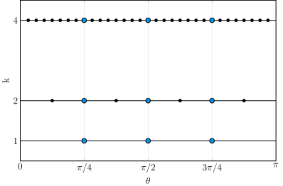
where nm=2m1(n1+1)1subscript𝑛𝑚superscript2𝑚1subscript𝑛111n_{m}=2^{m-1}(n_{1}+1)-1. In Figure 1 we show three grids, given by nk=2k1(n1+1)1subscript𝑛𝑘superscript2𝑘1subscript𝑛111n_{k}=2^{k-1}(n_{1}+1)-1, namely n1=3,n2=7formulae-sequencesubscript𝑛13subscript𝑛27n_{1}=3,n_{2}=7, and n4=31subscript𝑛431n_{4}=31. Blue circles indicate the sets of incices jksubscript𝑗𝑘j_{k} such that θjk,nksubscript𝜃subscript𝑗𝑘subscript𝑛𝑘\theta_{j_{k},n_{k}} always are the same for any k𝑘k.

Refer to caption
Figure 1: Three grids θj,nksubscript𝜃𝑗subscript𝑛𝑘\theta_{j,n_{k}} with k=1,2,4𝑘124k=1,2,4, nk=2k1(n1+1)1subscript𝑛𝑘superscript2𝑘1subscript𝑛111n_{k}=2^{k-1}(n_{1}+1)-1, and n1=3subscript𝑛13n_{1}=3. The subgrids θjk,nksubscript𝜃subscript𝑗𝑘subscript𝑛𝑘\theta_{j_{k},n_{k}}, which is the same for any k𝑘k, is indicated by blue circles (jk=2k1j1subscript𝑗𝑘superscript2𝑘1subscript𝑗1j_{k}=2^{k-1}j_{1}, j1={1,,n1}subscript𝑗11subscript𝑛1j_{1}=\{1,\ldots,n_{1}\}).

If we use the interpolation–extrapolation scheme introduced in [11], then we can approximate c~k(θj,n)subscript~𝑐𝑘subscript𝜃𝑗𝑛\tilde{c}_{k}(\theta_{j,n}) for any n𝑛n and thus we can compute numerically the full spectrum of Tn(f)subscript𝑇𝑛𝑓T_{n}(f) by

λj(Tn(f))λ~j(θ,α)(Tn(f))=f(θj,n)+k=1αc~k(θj,n)hk.subscript𝜆𝑗subscript𝑇𝑛𝑓superscriptsubscript~𝜆𝑗𝜃𝛼subscript𝑇𝑛𝑓𝑓subscript𝜃𝑗𝑛superscriptsubscript𝑘1𝛼subscript~𝑐𝑘subscript𝜃𝑗𝑛superscript𝑘\displaystyle\lambda_{j}(T_{n}(f))\approx\tilde{\lambda}_{j}^{(\theta,\alpha)}(T_{n}(f))=f(\theta_{j,n})+\sum_{k=1}^{\alpha}\tilde{c}_{k}(\theta_{j,n})h^{k}. (11)

Note that the procedure using the asymptotic expansion (11) also works for more general types of Toeplitz-like matrices, for example for preconditioned Toeplitz matrices [2], and block-Toeplitz matrices generated by matrix-valued symbols [10], and even in a differential setting when considering the isogeometric approximation of the Laplacian eigenvalue problem in any dimension [9]. The latter example is quite important since the involved matrices can be written as low-rank corrections of either of Toeplitz or of preconditioned Toeplitz matrices. We call this type of methods matrix-less since they do not need to construct a matrix, of arbitrary order n𝑛n, to approximate its eigenvalues (after the initial step when approximating ck(θj,n1)subscript𝑐𝑘subscript𝜃𝑗subscript𝑛1c_{k}(\theta_{j,n_{1}}) from α𝛼\alpha small matrices, data that can be reused for a matrix of any order).

By the notation of the theory of Generalized Locally Toeplitz (GLT) sequences, see [14] and references therein, we say that f𝑓f describes the eigenvalue distribution of a matrix Ansubscript𝐴𝑛A_{n}, when

{An}nglt,σ,λf.subscriptsimilar-toglt𝜎𝜆subscriptsubscript𝐴𝑛𝑛𝑓\displaystyle\{A_{n}\}_{n}\sim_{\textsc{glt},\sigma,\lambda}f.

Here we do not report the formal definitions for which we refer to [14], but instead we remind that {An}nσ,λfsubscriptsimilar-to𝜎𝜆subscriptsubscript𝐴𝑛𝑛𝑓\{A_{n}\}_{n}\sim_{\sigma,\lambda}f has the informal meaning that the bulk of singular values, eigenvalues behave, for n𝑛n large enough and up to infinitesimal errors in the parameter n𝑛n, as an equispaced sampling of the functions f𝑓f, |f|𝑓|f|, respectively over the common definition domain.

In this paper we consider the following types of matrices Ansubscript𝐴𝑛A_{n},

Ansubscript𝐴𝑛\displaystyle A_{n} =Tn(f),absentsubscript𝑇𝑛𝑓\displaystyle=T_{n}(f),
Ansubscript𝐴𝑛\displaystyle A_{n} =Tn(f)+Rn,absentsubscript𝑇𝑛𝑓subscript𝑅𝑛\displaystyle=T_{n}(f)+R_{n},
Ansubscript𝐴𝑛\displaystyle A_{n} =Tn1(b)Tn(a),f=a/b,formulae-sequenceabsentsuperscriptsubscript𝑇𝑛1𝑏subscript𝑇𝑛𝑎𝑓𝑎𝑏\displaystyle=T_{n}^{-1}(b)T_{n}(a),\quad f=a/b,

where f𝑓f is assumed to be real-valued, continuous and monotone, Rnsubscript𝑅𝑛R_{n} is a low-rank matrix, and a,b𝑎𝑏a,b are real-valued cosine polynomials, with b𝑏b non-negative and not identically zero. We thus have the following more general notation

λ~j(θ,α)(An)superscriptsubscript~𝜆𝑗𝜃𝛼subscript𝐴𝑛\displaystyle\tilde{\lambda}_{j}^{(\theta,\alpha)}(A_{n}) =f(θj,n)+k=1αc~k(θj,n)hk,absent𝑓subscript𝜃𝑗𝑛superscriptsubscript𝑘1𝛼subscript~𝑐𝑘subscript𝜃𝑗𝑛superscript𝑘\displaystyle=f(\theta_{j,n})+\sum_{k=1}^{\alpha}\tilde{c}_{k}(\theta_{j,n})h^{k}, (12)
E~j,n,αλ,θsuperscriptsubscript~𝐸𝑗𝑛𝛼𝜆𝜃\displaystyle\tilde{E}_{j,n,\alpha}^{\lambda,\theta} =λj(An)λ~j(α)(An).absentsubscript𝜆𝑗subscript𝐴𝑛superscriptsubscript~𝜆𝑗𝛼subscript𝐴𝑛\displaystyle=\lambda_{j}(A_{n})-\tilde{\lambda}_{j}^{(\alpha)}(A_{n}). (13)

2 Main Results

In this paper we now introduce the “perfect” grid ξj,nsubscript𝜉𝑗𝑛\xi_{j,n}, associated with the symbol f𝑓f and matrix Ansubscript𝐴𝑛A_{n}, such that

λj(An)=f(ξj,n),subscript𝜆𝑗subscript𝐴𝑛𝑓subscript𝜉𝑗𝑛\displaystyle\lambda_{j}(A_{n})=f(\xi_{j,n}), (14)

that is, sampling the symbol f(θ)𝑓𝜃f(\theta) with ξj,nsubscript𝜉𝑗𝑛\xi_{j,n} gives the exact eigenvalues of Ansubscript𝐴𝑛A_{n}. Such a grid has to exist thanks to the continuity of f𝑓f and thanks to the distributional/localization results (see [8] and references therein). We thus have

ξj,n=θj,n+Ej,nξ,subscript𝜉𝑗𝑛subscript𝜃𝑗𝑛superscriptsubscript𝐸𝑗𝑛𝜉\displaystyle\xi_{j,n}=\theta_{j,n}+E_{j,n}^{\xi}, (15)

where Ej,nξsuperscriptsubscript𝐸𝑗𝑛𝜉E_{j,n}^{\xi} is error in the sampling grid, using the standard grid (9) instead of the perfect grid ξj,nsubscript𝜉𝑗𝑛\xi_{j,n}. We now introduce the following fact, and dedicate the rest of this paper to show applications of this assumption to a number of different Toeplitz-like matrices and their symbols, describing the eigenvalue distribution. Fact 1 follows from (10) and from the monotonicity of f𝑓f via a proper Taylor expansion.

Fact 1.

There exists an expansion

ξj,n=θj,n+k=1αdk(θj,n)hk+Ej,n,αξ,subscript𝜉𝑗𝑛subscript𝜃𝑗𝑛superscriptsubscript𝑘1𝛼subscript𝑑𝑘subscript𝜃𝑗𝑛superscript𝑘superscriptsubscript𝐸𝑗𝑛𝛼𝜉\displaystyle\xi_{j,n}=\theta_{j,n}+\sum_{k=1}^{\alpha}d_{k}(\theta_{j,n})h^{k}+E_{j,n,\alpha}^{\xi}, (16)

where h=1/(n+1)1𝑛1h=1/(n+1), such that we can asymptotically describe a perfect grid ξj,nsubscript𝜉𝑗𝑛\xi_{j,n} such that (14) is true. Of course the latter holds for the same types of symbols for which the expansion (10) has been shown to work for; see for example [2, 10, 12].

We now first present two illustrative examples, and then propose Algorithm 1, a matrix-less method for approximating the functions dk(θ)subscript𝑑𝑘𝜃d_{k}(\theta) in (16). Finally Algorithm 2 describes how to use the information form Algorithm 1 to approximate the eigenvalues λj(An)subscript𝜆𝑗subscript𝐴𝑛\lambda_{j}(A_{n}) for any n𝑛n. Henceforth we use the following notation

ξ~j,n(α)superscriptsubscript~𝜉𝑗𝑛𝛼\displaystyle\tilde{\xi}_{j,n}^{(\alpha)} =θj,n+k=1αd~k(θj,n)hk,absentsubscript𝜃𝑗𝑛superscriptsubscript𝑘1𝛼subscript~𝑑𝑘subscript𝜃𝑗𝑛superscript𝑘\displaystyle=\theta_{j,n}+\sum_{k=1}^{\alpha}\tilde{d}_{k}(\theta_{j,n})h^{k}, (17)
E~j,n,αξsuperscriptsubscript~𝐸𝑗𝑛𝛼𝜉\displaystyle\tilde{E}_{j,n,\alpha}^{\xi} =ξj,nξ~j,n(α),absentsubscript𝜉𝑗𝑛superscriptsubscript~𝜉𝑗𝑛𝛼\displaystyle=\xi_{j,n}-\tilde{\xi}_{j,n}^{(\alpha)}, (18)
λ~j(ξ,α)(An)superscriptsubscript~𝜆𝑗𝜉𝛼subscript𝐴𝑛\displaystyle\tilde{\lambda}_{j}^{(\xi,\alpha)}(A_{n}) =f(ξj,n(α)),absent𝑓superscriptsubscript𝜉𝑗𝑛𝛼\displaystyle=f(\xi_{j,n}^{(\alpha)}), (19)
E~j,n,αλ,ξsuperscriptsubscript~𝐸𝑗𝑛𝛼𝜆𝜉\displaystyle\tilde{E}_{j,n,\alpha}^{\lambda,\xi} =λj(An)λ~j,n(ξ,α)(An),absentsubscript𝜆𝑗subscript𝐴𝑛superscriptsubscript~𝜆𝑗𝑛𝜉𝛼subscript𝐴𝑛\displaystyle=\lambda_{j}(A_{n})-\tilde{\lambda}_{j,n}^{(\xi,\alpha)}(A_{n}), (20)

to distinguish from the expansion and errors defined in (12) and (13).

Example 1.

In this example we study the symbol f(θ)=(22cos(θ))2=68cos(θ)+2cos(2θ)𝑓𝜃superscript22𝜃268𝜃22𝜃f(\theta)=(2-2\cos(\theta))^{2}=6-8\cos(\theta)+2\cos(2\theta), associated with the second order finite difference discretization of the bi-Laplacian. It is well known that an equispaced grid does not give the exact eigenvalues of the generated matrices Tn(f)subscript𝑇𝑛𝑓T_{n}(f) for finite matrices, for example, see discussions in [3, 13].

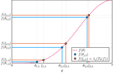
In Figure 2 we show the symbol f𝑓f (dashed pink line), and present data for the generated Toeplitz matrix of order n=3𝑛3n=3, T3(f)subscript𝑇3𝑓T_{3}(f), that is, the three eigenvalues λj(T3(f))=f(ξj,3)subscript𝜆𝑗subscript𝑇3𝑓𝑓subscript𝜉𝑗3\lambda_{j}(T_{3}(f))=f(\xi_{j,3}) (red circles) and the three samplings f(θj,3)𝑓subscript𝜃𝑗3f(\theta_{j,3}) (blue circles) where the sampling grid θj,3subscript𝜃𝑗3\theta_{j,3} is defined in (9).

Refer to caption
Figure 2: Example 1: Symbol f(θ)=(22cos(θ))2𝑓𝜃superscript22𝜃2f(\theta)=(2-2\cos(\theta))^{2} (dashed pink line) and the two expansions approximate the errors Ej,nλ,θ=λj(Tn(f))f(θj,n)=f(ξj,n)f(θj,n)superscriptsubscript𝐸𝑗𝑛𝜆𝜃subscript𝜆𝑗subscript𝑇𝑛𝑓𝑓subscript𝜃𝑗𝑛𝑓subscript𝜉𝑗𝑛𝑓subscript𝜃𝑗𝑛E_{j,n}^{\lambda,\theta}=\lambda_{j}(T_{n}(f))-f(\theta_{j,n})=f(\xi_{j,n})-f(\theta_{j,n}) and Ej,nξ=ξj,nθj,nsuperscriptsubscript𝐸𝑗𝑛𝜉subscript𝜉𝑗𝑛subscript𝜃𝑗𝑛E_{j,n}^{\xi}=\xi_{j,n}-\theta_{j,n}.

Hence, in previous papers, we approximate Ej,nλ,θsuperscriptsubscript𝐸𝑗𝑛𝜆𝜃E_{j,n}^{\lambda,\theta} in (8), by computing the λ~j(θ,α)(An)f(θj,n)superscriptsubscript~𝜆𝑗𝜃𝛼subscript𝐴𝑛𝑓subscript𝜃𝑗𝑛\tilde{\lambda}_{j}^{(\theta,\alpha)}(A_{n})-f(\theta_{j,n}) in (12). We thus approximate the error of the eigenvalue approximations when only using the symbol approximation f(θj,n)𝑓subscript𝜃𝑗𝑛f(\theta_{j,n}). The sought error Ej,3λ,θ=λj(T3(f))f(θj,3)superscriptsubscript𝐸𝑗3𝜆𝜃subscript𝜆𝑗subscript𝑇3𝑓𝑓subscript𝜃𝑗3E_{j,3}^{\lambda,\theta}=\lambda_{j}(T_{3}(f))-f(\theta_{j,3}) is the distance between the red and blue line on the y-axis.

In this paper we instead study the error Ej,nξsuperscriptsubscript𝐸𝑗𝑛𝜉E_{j,n}^{\xi} in (15), by computing the ξ~j,n(α)θj,nsuperscriptsubscript~𝜉𝑗𝑛𝛼subscript𝜃𝑗𝑛\tilde{\xi}_{j,n}^{(\alpha)}-\theta_{j,n} in (17). Hence, we approximate the error of the grid, when using the standard grid (9). The sought error Ej,3ξ=ξj,3θj,3superscriptsubscript𝐸𝑗3𝜉subscript𝜉𝑗3subscript𝜃𝑗3E_{j,3}^{\xi}=\xi_{j,3}-\theta_{j,3} is the distance between the red and blue line on the x-axis. Subsequently we can use the approximated ξ~j,n(α)superscriptsubscript~𝜉𝑗𝑛𝛼\tilde{\xi}_{j,n}^{(\alpha)}, in (17), to approximate the eigenvalues λj(Tn(f))subscript𝜆𝑗subscript𝑇𝑛𝑓\lambda_{j}(T_{n}(f)) by using (19).

In the following Example 2 we show the first numerical evidence supporting Fact 1.

Example 2.

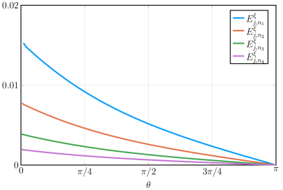
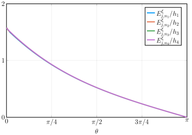
We return to the symbol f(θ)=(22cos(θ))2𝑓𝜃superscript22𝜃2f(\theta)=(2-2\cos(\theta))^{2} of Example 1. In Figure 3 we present in the left panel the errors Ej,nξ=Ej,n,0ξsuperscriptsubscript𝐸𝑗𝑛𝜉superscriptsubscript𝐸𝑗𝑛0𝜉E_{j,n}^{\xi}=E_{j,n,0}^{\xi} in (16), for a number of different n𝑛n, that is,

ξj,nsubscript𝜉𝑗𝑛\displaystyle\xi_{j,n} =cos1(2λj(Tn(f))2),absentsuperscript12subscript𝜆𝑗subscript𝑇𝑛𝑓2\displaystyle=\cos^{-1}\left(\frac{2-\sqrt{\lambda_{j}(T_{n}(f))}}{2}\right),
Ej,nξsuperscriptsubscript𝐸𝑗𝑛𝜉\displaystyle E_{j,n}^{\xi} =ξj,nθj,n.absentsubscript𝜉𝑗𝑛subscript𝜃𝑗𝑛\displaystyle=\xi_{j,n}-\theta_{j,n}.

The sizes of the matrices, used to compute Ej,nkξsuperscriptsubscript𝐸𝑗subscript𝑛𝑘𝜉E_{j,n_{k}}^{\xi} are nk=2k1(n1+1)1subscript𝑛𝑘superscript2𝑘1subscript𝑛111n_{k}=2^{k-1}(n_{1}+1)-1, where n1=100subscript𝑛1100n_{1}=100, and k=1,,4𝑘14k=1,\ldots,4. In the right panel we have scaled all the errors by hk=1/(nk+1)subscript𝑘1subscript𝑛𝑘1h_{k}=1/(n_{k}+1). The overlap is very good for the curves for different nksubscript𝑛𝑘n_{k}, indicating the general shape of d1(θ)subscript𝑑1𝜃d_{1}(\theta) in (16), later observed in Figure 5.

Refer to caption
Refer to caption
Figure 3: Example 2: Errors (Ej,nξ=ξj,nθj,n)superscriptsubscript𝐸𝑗𝑛𝜉subscript𝜉𝑗𝑛subscript𝜃𝑗𝑛(E_{j,n}^{\xi}=\xi_{j,n}-\theta_{j,n}) and scaled errors (Ej,nξ/h)superscriptsubscript𝐸𝑗𝑛𝜉(E_{j,n}^{\xi}/h). Left: Errors Ej,nkξsuperscriptsubscript𝐸𝑗subscript𝑛𝑘𝜉E_{j,n_{k}}^{\xi}, for nk=2k1(n1+1)1subscript𝑛𝑘superscript2𝑘1subscript𝑛111n_{k}=2^{k-1}(n_{1}+1)-1, n1=100subscript𝑛1100n_{1}=100, and k=1,,4𝑘14k=1,\ldots,4. Right: Scaled errors Ej,nkξ/hksuperscriptsubscript𝐸𝑗subscript𝑛𝑘𝜉subscript𝑘E_{j,n_{k}}^{\xi}/h_{k} where hk=1/(nk+1)subscript𝑘1subscript𝑛𝑘1h_{k}=1/(n_{k}+1).
Remark 1.

For more complicated symbols f𝑓f, the roots of f(θ)λj(An)𝑓𝜃subscript𝜆𝑗subscript𝐴𝑛f(\theta)-\lambda_{j}(A_{n}) are ξj,nsubscript𝜉𝑗𝑛\xi_{j,n}, and can be computed numerically.

We propose in Algorithm 1 a procedure for approximating dk(θ)subscript𝑑𝑘𝜃d_{k}(\theta) with d~k(θj,n1)subscript~𝑑𝑘subscript𝜃𝑗subscript𝑛1\tilde{d}_{k}(\theta_{j,n_{1}}), for k=1,,α𝑘1𝛼k=1,\ldots,\alpha on the grid points θj,n1subscript𝜃𝑗subscript𝑛1\theta_{j,n_{1}}, defined in (9). In Algorithm 2 we then use the interpolation–extrapolation scheme described in [11] to approximate dk(θj,n)subscript𝑑𝑘subscript𝜃𝑗𝑛d_{k}(\theta_{j,n}) for any n𝑛n, and subsequently use this data to approximate the eigenvalues λjAnsubscript𝜆𝑗subscript𝐴𝑛\lambda_{j}{A_{n}}. We here note that a similar approach was developed independently in [1].

Algorithm 1.

Approximate the expansion functions dk(θ)subscript𝑑𝑘𝜃d_{k}(\theta) in (16) in the points θj,n1subscript𝜃𝑗subscript𝑛1\theta_{j,n_{1}} defined in (9).

  1. 1.

    Choose n1subscript𝑛1n_{1} and α𝛼\alpha.

  2. 2.

    For each k=1,α𝑘1𝛼k=1,\ldots\alpha

    1. (a)

      Compute eigenvalues λj(Ank)subscript𝜆𝑗subscript𝐴subscript𝑛𝑘\lambda_{j}(A_{n_{k}}) where, for example,

      • Ank=Tnk(f)subscript𝐴subscript𝑛𝑘subscript𝑇subscript𝑛𝑘𝑓A_{n_{k}}=T_{n_{k}}(f),

      • Ank=Tnk(f)+Rnk+Nnksubscript𝐴subscript𝑛𝑘subscript𝑇subscript𝑛𝑘𝑓subscript𝑅subscript𝑛𝑘subscript𝑁subscript𝑛𝑘A_{n_{k}}=T_{n_{k}}(f)+R_{n_{k}}+N_{n_{k}},

      • Ank=(Tnk(b))1Tnk(a)subscript𝐴subscript𝑛𝑘superscriptsubscript𝑇subscript𝑛𝑘𝑏1subscript𝑇subscript𝑛𝑘𝑎A_{n_{k}}=(T_{n_{k}}(b))^{-1}T_{n_{k}}(a), f=a/b𝑓𝑎𝑏f=a/b,

      and nk=2k1(n1+1)1subscript𝑛𝑘superscript2𝑘1subscript𝑛111n_{k}=2^{k-1}(n_{1}+1)-1, Rnsubscript𝑅𝑛R_{n} is a low-rank matrix and Nnsubscript𝑁𝑛N_{n} is a small-norm matrix, a,b𝑎𝑏a,b are real-valued cosine polynomials, with b𝑏b non-negative and not identically zero; see [14];

    2. (b)

      Define the indices jk=2k1j1subscript𝑗𝑘superscript2𝑘1subscript𝑗1j_{k}=2^{k-1}j_{1}, where j1={1,,n1}subscript𝑗11subscript𝑛1j_{1}=\{1,\ldots,n_{1}\};

    3. (c)

      Compute the grid that gives the exact eigenvalues by finding the roots ξjk,nksubscript𝜉subscript𝑗𝑘subscript𝑛𝑘\xi_{j_{k},n_{k}} such that

      f(ξjk,nk)λjk(Ank)=0;𝑓subscript𝜉subscript𝑗𝑘subscript𝑛𝑘subscript𝜆subscript𝑗𝑘subscript𝐴subscript𝑛𝑘0\displaystyle f(\xi_{j_{k},n_{k}})-\lambda_{j_{k}}(A_{n_{k}})=0;
    4. (d)

      Store the errors in a matrix (𝐄)k,jk=ξjk,nkθj1,n1subscript𝐄𝑘subscript𝑗𝑘subscript𝜉subscript𝑗𝑘subscript𝑛𝑘subscript𝜃subscript𝑗1subscript𝑛1(\mathbf{E})_{k,j_{k}}=\xi_{j_{k},n_{k}}-\theta_{j_{1},n_{1}};

  3. 3.

    Create the Vandermonde matrix (𝐕)i,j=hijsubscript𝐕𝑖𝑗superscriptsubscript𝑖𝑗(\mathbf{V})_{i,j}=h_{i}^{j}, where hi=1/(ni+1)subscript𝑖1subscript𝑛𝑖1h_{i}=1/(n_{i}+1), where i,j=1,,αformulae-sequence𝑖𝑗1𝛼i,j=1,\ldots,\alpha;

  4. 4.

    Compute the 𝐃𝐃\mathbf{D} matrix by solving 𝐕𝐃=𝐄𝐕𝐃𝐄\mathbf{V}\mathbf{D}=\mathbf{E}, that is, 𝐃=𝐕\𝐄𝐃\𝐕𝐄\mathbf{D}=\mathbf{V}\backslash\mathbf{E}.

Once we have our 𝐃𝐃\mathbf{D} matrix, where d~k(θj,n1)=(𝐃)k,j1subscript~𝑑𝑘subscript𝜃𝑗subscript𝑛1subscript𝐃𝑘subscript𝑗1\tilde{d}_{k}(\theta_{j,n_{1}})=(\mathbf{D})_{k,j_{1}}, we can utilize them to reconstruct approximately the “perfect” grid ξj,nsubscript𝜉𝑗𝑛\xi_{j,n} for any n𝑛n. Hence, for an arbitrary n𝑛n, the full spectrum om Ansubscript𝐴𝑛A_{n} is then approximated by (19), by first using a modified version of the interpolation–extrapolation scheme of [11], to get d~k(θj,n)subscript~𝑑𝑘subscript𝜃𝑗𝑛\tilde{d}_{k}(\theta_{j,n}). The procedure is described in Algorithm 2.

Algorithm 2.

Compute approximation d~k(θj,n)subscript~𝑑𝑘subscript𝜃𝑗𝑛\tilde{d}_{k}(\theta_{j,n}) from d~k(θj,n1)subscript~𝑑𝑘subscript𝜃𝑗subscript𝑛1\tilde{d}_{k}(\theta_{j,n_{1}}), and approximate λj(An)subscript𝜆𝑗subscript𝐴𝑛\lambda_{j}(A_{n}).

  1. 1.

    Interpolate–extrapolate d~k(θj,n1)subscript~𝑑𝑘subscript𝜃𝑗subscript𝑛1\tilde{d}_{k}(\theta_{j,n_{1}}) to d~k(θj,n)subscript~𝑑𝑘subscript𝜃𝑗𝑛\tilde{d}_{k}(\theta_{j,n}) as is done for c~k(θj,n1)subscript~𝑐𝑘subscript𝜃𝑗subscript𝑛1\tilde{c}_{k}(\theta_{j,n_{1}}) in [11];

  2. 2.

    Compute ξ~j,n(α)=θj,n+k=1αd~k(θj,n)hksuperscriptsubscript~𝜉𝑗𝑛𝛼subscript𝜃𝑗𝑛superscriptsubscript𝑘1𝛼subscript~𝑑𝑘subscript𝜃𝑗𝑛superscript𝑘\tilde{\xi}_{j,n}^{(\alpha)}=\theta_{j,n}+\sum_{k=1}^{\alpha}\tilde{d}_{k}(\theta_{j,n})h^{k}, where h=1/(n+1)1𝑛1h=1/(n+1);

  3. 3.

    Compute the eigenvalue approximations λ~j(ξ,α)(An)=f(ξ~j,n(α))superscriptsubscript~𝜆𝑗𝜉𝛼subscript𝐴𝑛𝑓superscriptsubscript~𝜉𝑗𝑛𝛼\tilde{\lambda}_{j}^{(\xi,\alpha)}(A_{n})=f(\tilde{\xi}_{j,n}^{(\alpha)}).

3 Numerical Experiments

In this section we consider three different examples, numerically supporting Fact 1. In Example 3 we study the Toeplitz matrix associated with the second order finite difference discretization of the Laplacian, with imposed Neumann–Dirichlet boundary conditions. We examine in Example 4 the grid expansion (17) for the Toeplitz matrix associated with second order finite difference discretization of the bi-Laplacian. Finally the grid expansion (17) for a preconditioned matrix is presented in Example 5.

Example 3.

We here study the symbol f(θ)=22cos(θ)𝑓𝜃22𝜃f(\theta)=2-2\cos(\theta), and the perturbed generated matrix An=Tn(f)+Rnsubscript𝐴𝑛subscript𝑇𝑛𝑓subscript𝑅𝑛A_{n}=T_{n}(f)+R_{n} of the form

An=Tn(f)+Rn=[21121112]+[1]=[11121112].subscript𝐴𝑛subscript𝑇𝑛𝑓subscript𝑅𝑛delimited-[]21missing-subexpressionmissing-subexpressionmissing-subexpressionmissing-subexpressionmissing-subexpressionmissing-subexpressionmissing-subexpression121missing-subexpressionmissing-subexpressionmissing-subexpressionmissing-subexpressionmissing-subexpressionmissing-subexpressionmissing-subexpressionmissing-subexpressionmissing-subexpressionmissing-subexpressionmissing-subexpressionmissing-subexpressionmissing-subexpressionmissing-subexpression1missing-subexpressionmissing-subexpressionmissing-subexpressionmissing-subexpressionmissing-subexpressionmissing-subexpressionmissing-subexpression12missing-subexpressionmissing-subexpressionmissing-subexpressionmissing-subexpressiondelimited-[]1missing-subexpressionmissing-subexpressionmissing-subexpressionmissing-subexpressionmissing-subexpressionmissing-subexpressionmissing-subexpressionmissing-subexpressionmissing-subexpressionmissing-subexpressionmissing-subexpressionmissing-subexpressionmissing-subexpressionmissing-subexpressionmissing-subexpressionmissing-subexpressionmissing-subexpressionmissing-subexpressionmissing-subexpressionmissing-subexpressionmissing-subexpressionmissing-subexpressionmissing-subexpressionmissing-subexpressionmissing-subexpressionmissing-subexpressionmissing-subexpressionmissing-subexpressionmissing-subexpressionmissing-subexpressionmissing-subexpressionmissing-subexpressionmissing-subexpressionmissing-subexpressionmissing-subexpressiondelimited-[]11missing-subexpressionmissing-subexpressionmissing-subexpressionmissing-subexpressionmissing-subexpressionmissing-subexpressionmissing-subexpression121missing-subexpressionmissing-subexpressionmissing-subexpressionmissing-subexpressionmissing-subexpressionmissing-subexpressionmissing-subexpressionmissing-subexpressionmissing-subexpressionmissing-subexpressionmissing-subexpressionmissing-subexpressionmissing-subexpressionmissing-subexpression1missing-subexpressionmissing-subexpressionmissing-subexpressionmissing-subexpressionmissing-subexpressionmissing-subexpressionmissing-subexpression12missing-subexpressionmissing-subexpressionmissing-subexpressionmissing-subexpression\displaystyle A_{n}=T_{n}(f)+R_{n}=\left[\begin{array}[]{rrrrrrrrr}2&-1\\ -1&2&-1\\ &\ddots&\ddots&\ddots\\ &&\ddots&\ddots&-1\\ &&&-1&2\end{array}\right]+\left[\begin{array}[]{rrrrrrrrr}-1&\\ &\phantom{2}&\\ &\phantom{\ddots}&\phantom{\ddots}&\\ &&\phantom{\ddots}&&\\ &&&&\end{array}\right]=\left[\begin{array}[]{rrrrrrrrr}1&-1\\ -1&2&-1\\ &\ddots&\ddots&\ddots\\ &&\ddots&\ddots&-1\\ &&&-1&2\end{array}\right]. (36)

This matrix corresponds to the normalized discretization of second order finite differences och the second derivative operator (Laplacian), with imposed mixed Neumann–Dirichlet boundary conditions. It is known that the eigenvalues of Ansubscript𝐴𝑛A_{n} are exactly expressed by

λj(An)=f(ξj,n),ξj,n=(j1/2)πn+1/2,j=1,,n.formulae-sequencesubscript𝜆𝑗subscript𝐴𝑛𝑓subscript𝜉𝑗𝑛formulae-sequencesubscript𝜉𝑗𝑛𝑗12𝜋𝑛12𝑗1𝑛\displaystyle\lambda_{j}(A_{n})=f(\xi_{j,n}),\quad\xi_{j,n}=\frac{(j-1/2)\pi}{n+1/2},\quad j=1,\ldots,n.

We thus have

Ej,nξsuperscriptsubscript𝐸𝑗𝑛𝜉\displaystyle E_{j,n}^{\xi} =ξj,nθj,n=(j1/2)πn+1/2jπn+1=12n+1(θj,nπ),absentsubscript𝜉𝑗𝑛subscript𝜃𝑗𝑛𝑗12𝜋𝑛12𝑗𝜋𝑛112𝑛1subscript𝜃𝑗𝑛𝜋\displaystyle=\xi_{j,n}-\theta_{j,n}=\frac{(j-1/2)\pi}{n+1/2}-\frac{j\pi}{n+1}=\frac{1}{2n+1}\left(\theta_{j,n}-\pi\right),

and then

Ej,nξ=k=1dk(θj,n)hk,h=1/(n+1),formulae-sequencesuperscriptsubscript𝐸𝑗𝑛𝜉superscriptsubscript𝑘1subscript𝑑𝑘subscript𝜃𝑗𝑛superscript𝑘1𝑛1\displaystyle E_{j,n}^{\xi}=\sum_{k=1}^{\infty}d_{k}(\theta_{j,n})h^{k},\quad h=1/(n+1),

where

dk(θj,n)=12k(θj,nπ).subscript𝑑𝑘subscript𝜃𝑗𝑛1superscript2𝑘subscript𝜃𝑗𝑛𝜋\displaystyle d_{k}(\theta_{j,n})=\frac{1}{2^{k}}\left(\theta_{j,n}-\pi\right).

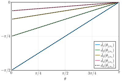
In Figure 4 we present d~k(θj,n1)subscript~𝑑𝑘subscript𝜃𝑗subscript𝑛1\tilde{d}_{k}(\theta_{j,n_{1}}), computed with Algorithm 1, and dk(θj,n1)subscript𝑑𝑘subscript𝜃𝑗subscript𝑛1d_{k}(\theta_{j,n_{1}}) for k=1,α𝑘1𝛼k=1,\ldots\alpha, for n1=100,α=4formulae-sequencesubscript𝑛1100𝛼4n_{1}=100,\alpha=4. The overlaps of the numerical and theoretical function values are good.
Refer to caption
Figure 4: Example 3: Expansion of the grid ξj,n1subscript𝜉𝑗subscript𝑛1\xi_{j,n_{1}} associated with the matrix An1=Tn1(f)+Rn1subscript𝐴subscript𝑛1subscript𝑇subscript𝑛1𝑓subscript𝑅subscript𝑛1A_{n_{1}}=T_{n_{1}}(f)+R_{n_{1}}, where f(θ)=22cos(θ)𝑓𝜃22𝜃f(\theta)=2-2\cos(\theta) and Rnsubscript𝑅𝑛R_{n} is a small rank perturbation (coming from a Neumann boundary condition). The functions dk(θ)subscript𝑑𝑘𝜃d_{k}(\theta) are well approximated by d~k(θ)subscript~𝑑𝑘𝜃\tilde{d}_{k}(\theta).
Example 4.

In this example we return to the symbol f𝑓f discussed in Examples 1 and 2, namely,

f(θ)=(22cos(θ))2=68cos(θ)+2cos(2θ),𝑓𝜃superscript22𝜃268𝜃22𝜃\displaystyle f(\theta)=(2-2\cos(\theta))^{2}=6-8\cos(\theta)+2\cos(2\theta),

and employ Algorithms 1 and 2 and study the results.

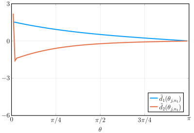
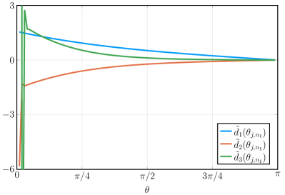
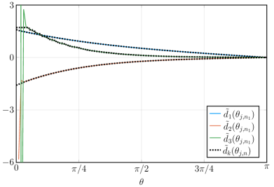
In Figure 5 we show the computed expansion functions d~k(θj,n1)subscript~𝑑𝑘subscript𝜃𝑗subscript𝑛1\tilde{d}_{k}(\theta_{j,n_{1}}), for n1=100subscript𝑛1100n_{1}=100 and α=2𝛼2\alpha=2 (left panel) and α=3𝛼3\alpha=3 (right panel). We note that for example d~2(θ1,n1)subscript~𝑑2subscript𝜃1subscript𝑛1\tilde{d}_{2}(\theta_{1,n_{1}}) and d~2(θ2,n1)subscript~𝑑2subscript𝜃2subscript𝑛1\tilde{d}_{2}(\theta_{2,n_{1}}) (red line, closest to θ=0𝜃0\theta=0) is different in the two panels. Also d~3(θj,n1)subscript~𝑑3subscript𝜃𝑗subscript𝑛1\tilde{d}_{3}(\theta_{j,n_{1}}) behaves erratic a few approximations close to θ=0𝜃0\theta=0. This effect is due to the fact that the symbol f𝑓f violates the simple-loop conditions, discussed in detail in [3] and also in [13]. However, this has low impact in the current numerical setting, and also we employ a modification of the extrapolation in [11] by simply ignoring user specified indices for the different k=1,,α𝑘1𝛼k=1,\ldots,\alpha.

Refer to caption
Refer to caption
Figure 5: Example 4: Computed expansion function approximations d~k(θj,n1)subscript~𝑑𝑘subscript𝜃𝑗subscript𝑛1\tilde{d}_{k}(\theta_{j,n_{1}}), k=1,,α𝑘1𝛼k=1,\ldots,\alpha for α=2𝛼2\alpha=2 (left) and α=3𝛼3\alpha=3 (right), and n1=100subscript𝑛1100n_{1}=100. Note the erratic behavior for d~2(θj,n1)subscript~𝑑2subscript𝜃𝑗subscript𝑛1\tilde{d}_{2}(\theta_{j,n_{1}}) and d~3(θj,n1)subscript~𝑑3subscript𝜃𝑗subscript𝑛1\tilde{d}_{3}(\theta_{j,n_{1}}) close to θ=0𝜃0\theta=0.

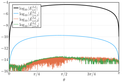
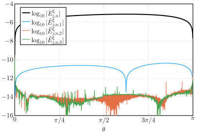
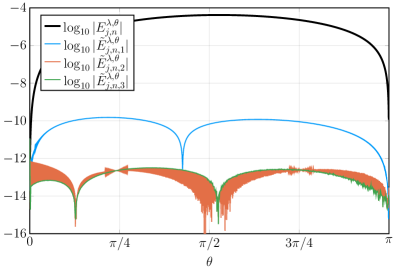
In the left panel of Figure 6 we show the interpolation–extrapolated d~k(θj,n)subscript~𝑑𝑘subscript𝜃𝑗𝑛\tilde{d}_{k}(\theta_{j,n}) (dashed black lines) for n1=100,α=3formulae-sequencesubscript𝑛1100𝛼3n_{1}=100,\alpha=3, and n=100000𝑛100000n=100000. The following samplings were ignored in these computations: for d~2(θj,n1)subscript~𝑑2subscript𝜃𝑗subscript𝑛1\tilde{d}_{2}(\theta_{j,n_{1}}) indices j=1,2𝑗12j=1,2 and for d~3(θj,n1)subscript~𝑑3subscript𝜃𝑗subscript𝑛1\tilde{d}_{3}(\theta_{j,n_{1}}) indices j=1,2,3𝑗123j=1,2,3. In the right panel of Figure 6 is presented the absolute error log10|Ej,nξ|subscript10superscriptsubscript𝐸𝑗𝑛𝜉\log_{10}|E_{j,n}^{\xi}| of (15) and the subsequent errors log10|E~j,n,βξ|subscript10superscriptsubscript~𝐸𝑗𝑛𝛽𝜉\log_{10}|\tilde{E}_{j,n,\beta}^{\xi}| of (18) for β=1,2,3𝛽123\beta=1,2,3. The perfect grid ξj,nsubscript𝜉𝑗𝑛\xi_{j,n} is very well approximated, with a slight reduction of accuracy close to θ=0𝜃0\theta=0. The parameters used for the computations in the right panel of Figure 6 (and also both panels of Figure 7) are n1=1000,α=3formulae-sequencesubscript𝑛11000𝛼3n_{1}=1000,\alpha=3, and n=100000𝑛100000n=100000. As expected the correction d~3(θj,n)h3subscript~𝑑3subscript𝜃𝑗𝑛superscript3\tilde{d}_{3}(\theta_{j,n})h^{3} to E~j,n,2ξsuperscriptsubscript~𝐸𝑗𝑛2𝜉\tilde{E}_{j,n,2}^{\xi} (to get E~j,n,3ξsuperscriptsubscript~𝐸𝑗𝑛3𝜉\tilde{E}_{j,n,3}^{\xi}) has only negligible effect since h3=𝒪(1015)superscript3𝒪superscript1015h^{3}=\mathcal{O}(10^{-15}). Only every 50thsuperscript50th50^{\mathrm{th}} (every 100thsuperscript100th100^{\mathrm{th}} for E~j,n,3ξsuperscriptsubscript~𝐸𝑗𝑛3𝜉\tilde{E}_{j,n,3}^{\xi}) error is plotted for improved clarity in the visualizations.
Refer to caption
Refer to caption
Figure 6: Example 4: Application of Algorithms 1 and 2,. Left: Approximations d~k(θj,n1)subscript~𝑑𝑘subscript𝜃𝑗subscript𝑛1\tilde{d}_{k}(\theta_{j,n_{1}}) from Algorithm 1 (colored lines) and d~k(θj,n)subscript~𝑑𝑘subscript𝜃𝑗𝑛\tilde{d}_{k}(\theta_{j,n}) from step 1 of of Algorithm 2 (dashed black lines). Right: The error Ej,nξsuperscriptsubscript𝐸𝑗𝑛𝜉E_{j,n}^{\xi} (and E~j,n,βξsuperscriptsubscript~𝐸𝑗𝑛𝛽𝜉\tilde{E}_{j,n,\beta}^{\xi}, for β=1,2,3)\beta=1,2,3).

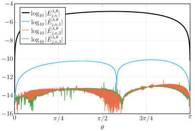
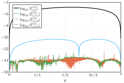
In Figure 7 we present the the errors Ej,nλ,θsuperscriptsubscript𝐸𝑗𝑛𝜆𝜃E_{j,n}^{\lambda,\theta} and Ej,nλ,ξsuperscriptsubscript𝐸𝑗𝑛𝜆𝜉E_{j,n}^{\lambda,\xi} (and E~j,n,βλ,θsuperscriptsubscript~𝐸𝑗𝑛𝛽𝜆𝜃\tilde{E}_{j,n,\beta}^{\lambda,\theta} and E~j,n,βλ,ξsuperscriptsubscript~𝐸𝑗𝑛𝛽𝜆𝜉\tilde{E}_{j,n,\beta}^{\lambda,\xi} for β=1,2,3𝛽123\beta=1,2,3) defined in (8) and (15) (and (13) and (20)). Thus, in the left panel of Figure 7 we show how well λj(Tn(f))subscript𝜆𝑗subscript𝑇𝑛𝑓\lambda_{j}(T_{n}(f)) are approximated using the method in [11] (with the addition of removal of erratic points in the interpolation–extrapolation stage). In the right panel of Figure 7 we present how well λj(Tn(f))subscript𝜆𝑗subscript𝑇𝑛𝑓\lambda_{j}(T_{n}(f)) are approximated using Algorithms 1 and 2 in this paper. We note that the result in the right panel is better overall for the whole spectrum, but especially close to θ=0𝜃0\theta=0, and machine precision accuracy has almost been achieved.
Refer to caption
Refer to caption
Figure 7: Example 4: Errors of eigenvalue approximations. Left: Errors log10|Ej,nλ,θ|subscript10superscriptsubscript𝐸𝑗𝑛𝜆𝜃\log_{10}|E_{j,n}^{\lambda,\theta}| (and log10|E~j,n,βλ,θ|subscript10superscriptsubscript~𝐸𝑗𝑛𝛽𝜆𝜃\log_{10}|\tilde{E}_{j,n,\beta}^{\lambda,\theta}|, for β=1,2,3𝛽123\beta=1,2,3). Computations using [11]. Right: Errors log10|Ej,nλ,ξ|subscript10superscriptsubscript𝐸𝑗𝑛𝜆𝜉\log_{10}|E_{j,n}^{\lambda,\xi}| (and log10|E~j,n,βλ,ξ|subscript10superscriptsubscript~𝐸𝑗𝑛𝛽𝜆𝜉\log_{10}|\tilde{E}_{j,n,\beta}^{\lambda,\xi}|, for β=1,2,3𝛽123\beta=1,2,3). Computations using Algorithms 1 and 2. Note the overall lower error compared with the left panel, especially close to θ=0𝜃0\theta=0.
Example 5.

Preconditioned matrices are important in many applications, and the study of their behavior is hence of importance. We here look at the matrix

Ansubscript𝐴𝑛\displaystyle A_{n} =Tn1(a)Tn(b),absentsuperscriptsubscript𝑇𝑛1𝑎subscript𝑇𝑛𝑏\displaystyle=T_{n}^{-1}(a)T_{n}(b),
{An}subscript𝐴𝑛\displaystyle\{A_{n}\} glt,σ,λf,subscriptsimilar-toglt𝜎𝜆absent𝑓\displaystyle\sim_{\textsc{glt},\sigma,\lambda}f,

where

a(θ)𝑎𝜃\displaystyle a(\theta) =42cos(θ)2cos(2θ)=(22cos(θ))(3+2cos(θ)),absent42𝜃22𝜃22𝜃32𝜃\displaystyle=4-2\cos(\theta)-2\cos(2\theta)=(2-2\cos(\theta))(3+2\cos(\theta)),
b(θ)𝑏𝜃\displaystyle b(\theta) =3+2cos(θ),absent32𝜃\displaystyle=3+2\cos(\theta),
f(θ)𝑓𝜃\displaystyle f(\theta) =a(θ)/b(θ)=22cos(θ),absent𝑎𝜃𝑏𝜃22𝜃\displaystyle=a(\theta)/b(\theta)=2-2\cos(\theta),

which is Example 1 from [2].

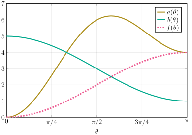
In the left panel of Figure 8 we show the symbols a,b𝑎𝑏a,b, and f=a/b𝑓𝑎𝑏f=a/b. In the right panel of Figure 8 is shown the absolute error when approximating ξj,nsubscript𝜉𝑗𝑛\xi_{j,n}, that is, log10|Ej,nξ|subscript10superscriptsubscript𝐸𝑗𝑛𝜉\log_{10}|E_{j,n}^{\xi}| (and log10|E~j,n,βξ|subscript10superscriptsubscript~𝐸𝑗𝑛𝛽𝜉\log_{10}|\tilde{E}_{j,n,\beta}^{\xi}| for β=1,2,3𝛽123\beta=1,2,3). Like in the right panel of Figure 6 we note a slight reduction of accuracy close to θ=0𝜃0\theta=0, but here also close to θ=π𝜃𝜋\theta=\pi.

Refer to caption
Refer to caption
Figure 8: Example 5: Symbols and errors approximating ξj,nsubscript𝜉𝑗𝑛\xi_{j,n}. Left: Symbols a,b𝑎𝑏a,b, and f=a/b𝑓𝑎𝑏f=a/b. Right: log10|Ej,nξ|subscript10superscriptsubscript𝐸𝑗𝑛𝜉\log_{10}|E_{j,n}^{\xi}| (and log10|E~j,n,βξ|subscript10superscriptsubscript~𝐸𝑗𝑛𝛽𝜉\log_{10}|\tilde{E}_{j,n,\beta}^{\xi}| for β=1,2,3𝛽123\beta=1,2,3 for n1=1000,α=3formulae-sequencesubscript𝑛11000𝛼3n_{1}=1000,\alpha=3, and n=100000𝑛100000n=100000).

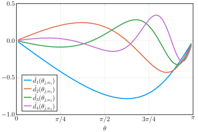
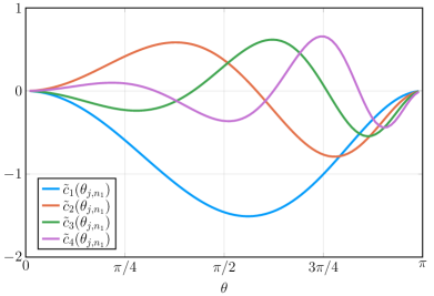
In Figure 9 we present both the computed expansion function c~k(θj,n)subscript~𝑐𝑘subscript𝜃𝑗𝑛\tilde{c}_{k}(\theta_{j,n}) (left) and d~k(θj,n)subscript~𝑑𝑘subscript𝜃𝑗𝑛\tilde{d}_{k}(\theta_{j,n}) (right). We note the similarity between the two expansions.
Refer to caption
Refer to caption
Figure 9: Example 5: Expansions for preconditioned matrix, n1=100subscript𝑛1100n_{1}=100 and α=4𝛼4\alpha=4. Left: Expansion c~k(θj,n1)subscript~𝑐𝑘subscript𝜃𝑗subscript𝑛1\tilde{c}_{k}(\theta_{j,n_{1}}), for k=1,,α𝑘1𝛼k=1,\ldots,\alpha. Right: Expansion d~k(θj,n1)subscript~𝑑𝑘subscript𝜃𝑗subscript𝑛1\tilde{d}_{k}(\theta_{j,n_{1}}), for k=1,,4𝑘14k=1,\ldots,4.

Finally in Figure 10 we present the absolute errors when approximating λj(Tn1(b)Tn(a))subscript𝜆𝑗superscriptsubscript𝑇𝑛1𝑏subscript𝑇𝑛𝑎\lambda_{j}(T_{n}^{-1}(b)T_{n}(a)), that is, log10|Ej,nλ,θ|subscript10superscriptsubscript𝐸𝑗𝑛𝜆𝜃\log_{10}|E_{j,n}^{\lambda,\theta}| (left panel) and log10|Ej,nλ,ξ|subscript10superscriptsubscript𝐸𝑗𝑛𝜆𝜉\log_{10}|E_{j,n}^{\lambda,\xi}| (right panel) (and log10|E~j,n,βλ,θ|subscript10superscriptsubscript~𝐸𝑗𝑛𝛽𝜆𝜃\log_{10}|\tilde{E}_{j,n,\beta}^{\lambda,\theta}| and log10|E~j,n,βλ,ξ|subscript10superscriptsubscript~𝐸𝑗𝑛𝛽𝜆𝜉\log_{10}|\tilde{E}_{j,n,\beta}^{\lambda,\xi}| for β=1,2,3𝛽123\beta=1,2,3). As is noted in Figure 7, the Algorithms 1 and 2 generally perform better than the algorithm in [11]. The additional cost for Algorithms 1 and 2, compared with [11], is negligible. It consists only of finding the αn1𝛼subscript𝑛1\alpha n_{1} roots to f(θ)λjk(Ank)𝑓𝜃subscript𝜆subscript𝑗𝑘subscript𝐴subscript𝑛𝑘f(\theta)-\lambda_{j_{k}}(A_{n_{k}}), for k=1,,α𝑘1𝛼k=1,\ldots,\alpha.

Refer to caption
Refer to caption
Figure 10: Example 5: Errors of eigenvalue approximations. Left: Errors log10|Ej,nλ,θ|subscript10superscriptsubscript𝐸𝑗𝑛𝜆𝜃\log_{10}|E_{j,n}^{\lambda,\theta}| (and log10|E~j,n,βλ,θ|subscript10superscriptsubscript~𝐸𝑗𝑛𝛽𝜆𝜃\log_{10}|\tilde{E}_{j,n,\beta}^{\lambda,\theta}|, for β=1,2,3𝛽123\beta=1,2,3). Computations using [11]. Right: Errors log10|Ej,nλ,ξ|subscript10superscriptsubscript𝐸𝑗𝑛𝜆𝜉\log_{10}|E_{j,n}^{\lambda,\xi}| (and log10|E~j,n,βλ,ξ|subscript10superscriptsubscript~𝐸𝑗𝑛𝛽𝜆𝜉\log_{10}|\tilde{E}_{j,n,\beta}^{\lambda,\xi}|, for β=1,2,3𝛽123\beta=1,2,3). Computations using Algorithms 1 and 2. Note the overall lower error compared with the left panel.

4 Conclusions

In this paper we have studied the expansion of the grid error Ej,nξsuperscriptsubscript𝐸𝑗𝑛𝜉E_{j,n}^{\xi} in ξj,n=θj,n+Ej,nξsubscript𝜉𝑗𝑛subscript𝜃𝑗𝑛superscriptsubscript𝐸𝑗𝑛𝜉\xi_{j,n}=\theta_{j,n}+E_{j,n}^{\xi}, where ξj,nsubscript𝜉𝑗𝑛\xi_{j,n} is the “perfect” grid associated with a sequence of matrices {An}nsubscriptsubscript𝐴𝑛𝑛\{A_{n}\}_{n}, in the sense that λj(An)=f(ξj,n)subscript𝜆𝑗subscript𝐴𝑛𝑓subscript𝜉𝑗𝑛\lambda_{j}(A_{n})=f(\xi_{j,n}). Here f𝑓f is the symbol such that {An}nglt,σ,λfsubscriptsimilar-toglt𝜎𝜆subscriptsubscript𝐴𝑛𝑛𝑓\{A_{n}\}_{n}\sim_{\textsc{glt},\sigma,\lambda}f. We present an Algorithm 1 to approximate the expansion, proposed in Fact 1, of the error Ej,nξsuperscriptsubscript𝐸𝑗𝑛𝜉E_{j,n}^{\xi} in (16). In Algorithm 2 we show how to interpolate–extrapolate the data from Algorithm 1, and use this information to approximate the eigenvalues of Ansubscript𝐴𝑛A_{n} for arbitrary n𝑛n. By the numerical experiments in Section 3 we have shown evidence of Fact 1, in a number of practical examples, by also emphasizing the superiority of the new matrix-less method seen in Examples 4 and 5 when approximating the eigenvalues of a large matrix Ansubscript𝐴𝑛A_{n}.

The further study of the proposed expansion is warranted, since it might lead to new discoveries on the spectral behavior by applying perturbations of Toeplitz-like matrices, and also faster and more accurate methods to approximate the spectrum of Toeplitz-like matrices. For matrices generated by partially non-monotone symbols we expect similar behavior as for the expansion of the eigenvalue errors: in particular the conclusion is that we can not in general gain any information in the non-monotone part. The block and multilevel cases are also to be considered in future research.

5 Acknowledgments

The author would like to thank Stefano Serra-Capizzano for valuable discussions and suggestions during the preparation of this work. The author is financed by Athens University of Economics and Business.

References

  • [1] F. Ahmad, Equations and Systems of Nonlinear Equations: from high order Numerical Methods to fast Eigensolvers for Structured Matrices and Applications, PhD thesis, University of Insubria, 2018.
  • [2] F. Ahmad, E. S. Al-Aidarous, D. A. Alrehaili, S.-E. Ekström, I. Furci, and S. Serra-Capizzano, Are the eigenvalues of preconditioned banded symmetric Toeplitz matrices known in almost closed form?, Numerical Algorithms, 78 (2017), pp. 867–893.
  • [3] M. Barrera, A. Böttcher, S. M. Grudsky, and E. A. Maximenko, Eigenvalues of even very nice Toeplitz matrices can be unexpectedly erratic, in The Diversity and Beauty of Applied Operator Theory, Springer International Publishing, 2018, pp. 51–77.
  • [4] J. Bogoya, A. Böttcher, S. Grudsky, and E. Maximenko, Eigenvalues of Hermitian Toeplitz matrices with smooth simple-loop symbols, Journal of Mathematical Analysis and Applications, 422 (2015), pp. 1308–1334.
  • [5] J. M. Bogoya, S. M. Grudsky, and E. A. Maximenko, Eigenvalues of Hermitian Toeplitz Matrices Generated by Simple-loop Symbols with Relaxed Smoothness, in Large Truncated Toeplitz Matrices, Toeplitz Operators, and Related Topics, Springer International Publishing, 2017, pp. 179–212.
  • [6] A. Böttcher, S. Grudsky, and E. Maksimenko, Inside the eigenvalues of certain Hermitian Toeplitz band matrices, Journal of Computational and Applied Mathematics, 233 (2010), pp. 2245–2264.
  • [7] A. Böttcher and B. Silbermann, Introduction to Large Truncated Toeplitz Matrices, Springer New York, 1999.
  • [8] F. Di Benedetto, G. Fiorentino, and S. Serra, C. G. preconditioning for Toeplitz matrices, Computers & Mathematics with Applications, 25 (1993), pp. 35–45.
  • [9] S.-E. Ekström, I. Furci, C. Garoni, C. Manni, S. Serra-Capizzano, and H. Speleers, Are the eigenvalues of the B-spline isogeometric analysis approximation of Δu=λuΔ𝑢𝜆𝑢-\Delta u=\lambda u known in almost closed form?, Numerical Linear Algebra with Applications, 25 (2018), p. e2198.
  • [10] S.-E. Ekström, I. Furci, and S. Serra-Capizzano, Exact formulae and matrix-less eigensolvers for block banded symmetric Toeplitz matrices, BIT Numerical Mathematics, 58 (2018), pp. 937–968.
  • [11] S.-E. Ekström and C. Garoni, A matrix-less and parallel interpolation–extrapolation algorithm for computing the eigenvalues of preconditioned banded symmetric Toeplitz matrices, Numerical Algorithms, (2018). https://doi.org/10.1007/s11075-018-0508-0, (in press).
  • [12] S.-E. Ekström, C. Garoni, and S. Serra-Capizzano, Are the Eigenvalues of Banded Symmetric Toeplitz Matrices Known in Almost Closed Form?, Experimental Mathematics, 27 (2018), pp. 478–487.
  • [13] S.-E. Ekström, Matrix-Less Methods for Computing Eigenvalues of Large Structured Matrices, PhD thesis, Uppsala University, Uppsala: Acta Universitatis Upsaliensis, 2018.
  • [14] C. Garoni and S. Serra-Capizzano, Generalized Locally Toeplitz Sequences: Theory and Applications (Volume 1), Springer International Publishing, 2017.