Optimal Task Scheduling Benefits From a Duplicate-Free State-Space

Abstract

The NP-hard problem of task scheduling with communication delays ($P|prec,c_{ij}|C_{\mathrm{max}}$) is often tackled using approximate methods, but guarantees on the quality of these heuristic solutions are hard to come by. Optimal schedules are therefore invaluable for properly evaluating these heuristics, as well as being very useful for applications in time critical systems. Optimal solving using branch-and-bound algorithms like A* has been shown to be promising in the past, with a state-space model we refer to as exhaustive list scheduling (ELS). The obvious weakness of this model is that it leads to the production of large numbers of duplicate states during a search, requiring special techniques to mitigate this which cost additional time and memory. In this paper we define a new state-space model (AO) in which we divide the problem into two distinct sub-problems: first we decide the allocations of all tasks to processors, and then we order the tasks on their allocated processors in order to produce a complete schedule. This two-phase state-space model offers no potential for the production of duplicates. We also describe how the pruning techniques and optimisations developed for the ELS model were adapted or made obsolete by the AO model. An experimental evaluation shows that the use of this new state-space model leads to a significant increase in the number of task graphs able to be scheduled within a feasible time-frame, particularly for task graphs with a high communication-to-computation ratio. Finally, some advanced lower bound heuristics are proposed for the AO model, and evaluation demonstrates that significant gains can be achieved from the consideration of necessary idle time.

Department of Electrical and Computer Engineering, University of Auckland, New Zealand

1 Introduction

In order to use the full potential of a multiprocessor system in speeding up task execution, efficient schedules are required. In this work, we address the classic problem of task scheduling with communication delays, known as $P|prec,c_{ij}|C_{\mathrm{max}}$ using the $\alpha|\beta|\gamma$ notation [1]. The problem involves a set of tasks, with associated precedence constraints and communication delays, which must be scheduled such that the overall finish time (schedule length) is minimised. The optimal solving of this problem is well known to be NP-hard [2], so that the amount of work required grows exponentially as the number of tasks is increased. For this reason, many heuristic approaches have been developed, trading solution quality for reduced computation time [3, 4, 5, 6]. Unfortunately, the relative quality of these approximate solutions cannot be guaranteed, as no $\alpha$-approximation scheme for the problem is known [7].

Although the NP-hardness of the problem usually discourages optimal solving, an optimal schedule can give a significant advantage in time critical systems or applications where a single schedule is reused many times. Optimal solutions are also necessary in order to evaluate the effectiveness of a heuristic scheduling method. Branch-and-bound algorithms have previously shown promise in efficiently finding optimal solutions to this problem [8], but the state-space model used, exhaustive list scheduling (ELS), was prone to the production of duplicate states.

This paper presents a new state-space model in which the task scheduling problem is tackled in two distinct phases: first allocation, and then ordering. The two-phase state-space model (abbreviated AO) does not allow for the possibility of duplicate states. We give a detailed explanation of the algorithms and heuristics used to explore the AO state space and discuss its theoretical benefits over ELS, as well as its limitations. We describe the algorithms necessary to guarantee that all valid states can be produced, and that invalid states cannot. Previous research demonstrated that the ELS model benefited immensely from the application of pruning techniques such as processor normalisation and identical task pruning. The benefit is such that effective pruning would seem to be a necessity in order for another model to be competitive. We therefore describe these techniques and explain the changes needed to adapt them from the ELS model to the AO model. An experimental evaluation is used to compare the performance of the two state-space models. We then propose further advances to lower bound heuristics for AO, and evaluate these. This paper expands on preliminary work, which featured a promising evaluation using only small task graphs [9].

In Section 2, background information is given, including an explanation of the task scheduling model, an overview of branch-and-bound algorithms, and a description of the ELS model. Section 4 describes the new AO model, and how a branch-and-bound search is conducted through it. Section 5 proposes a technique to avoid searching invalid states in the ordering phase. Section 6 explains the pruning techniques used with ELS, and their adaptation to the AO model. Section 7 explains how the new model was evaluated by comparison with the old one, and presents the results. Section 8 describes novel and more complex lower bound heuristics for the AO model, and an evaluation of their effect. Finally, Section 9 gives the conclusions of the paper and outlines possible further avenues of study.

2 Background

2.1 Task Scheduling Model

The specific problem that we address here is the scheduling of a task graph $G=\{V,E,w,c\}$ on a set of processors $P$. $G$ is a directed acyclic graph wherein each node $n\in V$ represents a task, and each edge $e_{ij}\in E$ represents a required communication from task $n_{i}$ to task $n_{j}$. Figure 1 shows an example of a task graph. The computation cost of a task $n\in V$ is given by its positive weight $w(n)$, and the communication cost of an edge $e_{ij}\in E$ is given by the non-negative weight $c(e_{ij})$. The target parallel system for our schedule consists of a finite number of homogeneous processors, represented by $P$. Each processor is dedicated, meaning that no executing task may be preempted. We assume a fully connected communication subsystem, such that each pair of processors $p_{i},p_{j}\in P$ is connected by an identical communication link. Communications are performed concurrently and without contention. Local communication (from $p_{i}$ to $p_{i}$) is assumed to take place in the memory shared by the tasks on the same processor and is therefore assumed to have zero cost.

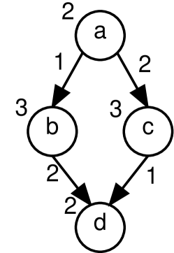
Figure 1: A simple task graph.

Our aim is to produce a schedule $S=\{proc,t_{\mathrm{s}}\}$, where $proc(n)$ allocates the task to a processor in $P$, and $t_{\mathrm{s}}(n)$ assigns it a start time on this processor. For a schedule to be valid, it must fulfill two conditions for all tasks in $G$. The Processor Constraint requires that only one task is executed by a processor at any one time. The Precedence Constraint requires that a task $n$ may only be executed once all of its predecessors have finished execution, and all required data has been communicated to $proc(n)$. Figure 2 illustrates a valid schedule for the task graph in Figure 1. The goal of optimal task scheduling is to find such a schedule $S$ for which the total execution time or schedule length $sl(S)$ is the lowest possible.

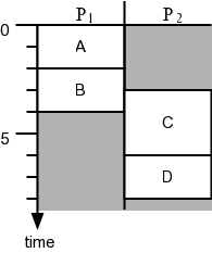
Figure 2: A valid schedule for the simple task graph of Fig..

It is useful to define the concept of node levels for a task graph [6]. For a task $n$, the top level $tl(n)$ is the length of the longest path in the task graph that ends with $n$. This does not include the weight of $n$, or any communication costs. Similarly, the bottom level $bl(n)$ is the length of the longest path beginning with $n$, excluding communication costs. The weight of $n$ is included in $bl(n)$. The allocated top and bottom levels $tl_{\alpha}(n)$ and $bl_{\alpha}(n)$ incorporate communication costs, once the allocation of a parent and child task to different processors confirms that the edge between them will be incurred.

Task graphs can be categorised into a number of different structures, which often have distinct properties and associated difficulties when solving. Figure 3 shows examples of some of the simplest structures.

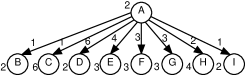
(a) Fork

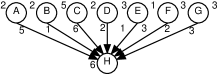
(b) Join

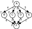
(c) Fork-join

Figure 3: Example of simple task graph structures

2.2 Branch-and-Bound

The term branch-and-bound refers to a family of search algorithms which are widely used for the solving of combinatorial optimisation problems. They do this by implicitly enumerating all solutions to a problem, simultaneously finding an optimal solution and proving its optimality [10]. A search tree is constructed in which each node (usually referred to as a state) represents a partial solution to the problem. From the partial solution represented by a state $s$, some set of operations is applied to produce new partial solutions which are closer to a complete solution. In this way we define the children of $s$, and thereby branch. Each state must also be bounded: we evaluate each state $s$ using a cost function $f$, such that $f(s)$ is a lower bound on the cost of any solution that can be reached from $s$. Using these bounds, we can guide our search away from unpromising partial solutions and therefore remove large subsets of the potential solutions from the need to be fully examined.

A* is a particularly popular variant of branch-and-bound which uses a best-first search approach [11]. A* has the interesting property that it is optimally efficient; using the same cost function $f$, no search algorithm could find an optimal solution while examining fewer states. To achieve this property, it is necessary that the cost function $f$ provides an underestimate. That is, it must be the case that $f(s)\leq f^{*}(s)$, where $f^{*}(s)$ is the true lowest cost of a complete solution in the sub-tree rooted at $s$. A cost function with this property is said to be admissable.

2.3 Exhaustive List Scheduling

Previous branch-and-bound approaches to optimal task scheduling have used a state-space model that is inspired by list scheduling algorithms [8]. States are partial schedules in which some subset of the tasks in the problem instance have been assigned to a processor and given a start time. At each branching step, successors are created by putting every possible ready task (tasks for which all parents are already scheduled) on every possible processor at the earliest possible start time. In this way, the search space demonstrates every possible sequence of decisions that a list scheduling algorithm could make. This branch-and-bound strategy can therefore be described as exhaustive list scheduling. Figure 4 demonstrates how four possible child states can be reached from a partial schedule with two ready tasks and two processors.

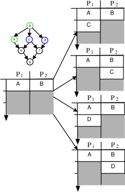
Figure 4: Branching in the ELS state space.

Branch-and-bound works most efficiently when the sub-trees produced when branching are entirely disjoint. Another way of stating this is that there is only one possible path from the root of the tree to any given state, and therefore there is only one way in which a search can create this state. When this is not the case, a large amount of work can be wasted: the same state could be expanded, and its sub-tree subsequently explored, multiple times. Avoiding this requires doing work to detect duplicate states, such as keeping a set of already created states with which all new states must be compared. This process increases the algorithm’s need for both time and memory.

Unfortunately, the ELS strategy creates a lot of potential for duplicated states [12]. This stems from two main sources:

Processor Permutation Duplicates

Firstly, since the processors are homogeneous, any permutation of the processors in a schedule represents an entirely equivalent schedule. For example, Figure 5 shows two partial schedules which are identical aside from the labelling of the processors. This means that for each truly unique complete schedule, there will be $|P|!$ equivalent complete schedules in the state space. This makes it very important to use some strategy of processor normalisation when branching, such that these equivalent states cannot be produced.

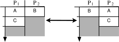
Figure 5: Processor permutation duplicates.

Independent Decision Duplicates

The other source of duplicate states is more difficult to deal with. When tasks are independent of each other, the order in which they are selected for scheduling can be changed without affecting the resulting schedule. This means there is more than one path to the corresponding state, and therefore a potential duplicate. Figure 6 demonstrates how multiple paths can lead to the same state. The only way to avoid these duplicates is to enforce a particular sequence onto these scheduling decisions. Under the ELS strategy, however, no method is apparent in which this could be achieved while also allowing all possible legitimate schedules to be produced.

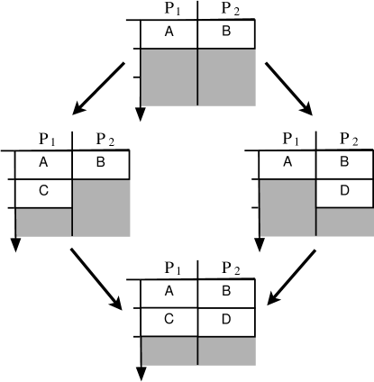
Figure 6: Independent decision duplicates.

3 Related Work

Although the task scheduling model presented here can be applied to the parallelisation of any arbitrary program, one specific area to which task scheduling has been practically applied in recent years is in the implementation of linear algebra solvers. Software packages such as SuperMatrix[13] and PLASMA[14] represent linear algebra algorithms as DAGs, decomposing the steps required into tasks, and use a variety of methods to schedule these graphs. They do not, however, attempt to find optimal schedules, although this could be helpful in some specific circumstances.

Due to the NP-hard nature of the task scheduling problem, the majority of efforts have gone towards developing polynomial-time heuristic solutions, producing schedules which are “good enough” for most applications. The two major categories of approximation algorithms are list scheduling and clustering [6]. List scheduling algorithms generally proceed in two phases: first, all of the tasks are placed into an ordered list, according to some priority scheme. Second, the tasks are removed from the list one by one, in order, and scheduled. That is, they are assigned to a processor, and usually given a start time as early as possible after the tasks previously assigned to that processor have completed. Notable list scheduling variants include MCP[15] and HLFET[16]. In a clustering algorithm, tasks are grouped together in clusters, with the intention that if two tasks belong to the same cluster then it is likely to be beneficial for them to be assigned to the same processor. Technically, a clustering algorithm is only concerned with suggesting a processor allocation for the tasks, with a subsequent process similar to list scheduling usually required in order to produce an actual schedule. Notable clustering variants include DCP[17] and DSC[18]. While the ELS model resembles a generalised version of the list scheduling approach (hence its name), the new AO model more closely resembles a clustering approach.

The task scheduling problem is theoretically susceptible to many combinatorial optimisation techniques. A*, the popular branch-and-bound search algorithm, has been successfully applied to the optimal solving of small problem instances through the ELS model [8] and earlier attempts [19]. Another combinatorial optimisation technique which has been applied to this task scheduling problem is integer linear programming (ILP). This involves formulating the problem instance as a linear program, a series of simultaneous linear equations, where the variables are constrained to integer values. A number of possible ILP formulations of the $P|prec,c_{ij}|C_{\mathrm{max}}$ problem have been proposed [20, 21, 22], with similarly promising results as branch-and-bound. Neither technique has been shown to have a significant advantage over the other in terms of the size of task scheduling problem that they can solve practically. Most widely used ILP solvers are mature, highly optimised, proprietary software packages. This optimisation means they are very likely to have a built-in advantage in terms of speed when compared to a custom implementation of state-space search. On the other hand, their complexity and proprietary nature make them somewhat of a “black box”. A custom implementation makes it easier to gain potentially critical insight into the behaviour of the solver. Additionally, it is often easier to map domain-specific knowledge directly into a state-space model than into an ILP formulation.

Many combinatorial optimisation problems can be naturally expressed as permutation problems, meaning that the set of solutions consists of all possible arrangements or orderings of some set of objects. In the most famous of these, the travelling salesperson problem (TSP), the goal is to plan a trip which visits a number of cities such that the total distance travelled between the cities is minimised [23]. Evidently, each possible ordering of the cities represents a valid solution, and the optimal solution can be found by iterating over these permutations. Other classic permutation problems include the assignment problem [24] and the MAX-SAT problem [25]. Another class of combinatorial optimisation problem can be thought of as a distribution or allocation problem, in which a set of objects must be divided among a number of possible groups. Examples include the graph colouring problem [26], and the problem of task scheduling with independent tasks [6].

The problem of task scheduling with communication delays is interesting in that it can be considered as the composition of a distribution problem with a permutation problem, as the tasks must both be optimally divided among the processors and ordered optimally on each processor. An example of a similar problem is that of minimizing part programs for numerical control (NC) punch presses, which could be decomposed into two distinct permutation problems (TSP and the assignment problem), A proposed algorithm for this problem iterated between these two sub-problems, using heuristic approaches to solve each [27]. To the best of our knowledge, our proposed model is the first to attempt optimal solving by branch-and-bound through separating two subproblems into distinct phases, which are combined into one overall solution space.

Pruning techniques are considered to be a fundamental aspect of branch-and-bound search, as they have the potential to greatly limit the number of states that need to be evaluated [28]. Work on pruning techniques for the ELS model demonstrated that they had a dramatic impact on its performance [12]. It seems unlikely that any state-space model could be competitive without the development of effective pruning techniques.

4 Duplicate-Free State-Space Model

Both sources of duplicate states can be eliminated by adopting a new state-space model (AO), in which the two dimensions of task scheduling are dealt with separately. Rather than making all decisions about a task’s placement simultaneously, the search proceeds in two stages. In the first stage, we decide for each task the processor to which it will be assigned. We refer to this as the allocation phase. The second stage of the search, beginning after all tasks are allocated, decides the start time of each task. Given that each processor has a known set of tasks allocated to it, this is equivalent to deciding on an ordering for each set. Therefore, we refer to this as the ordering phase. Once the allocation phase has determined the tasks’ positions in space, and the ordering phase has determined the tasks’ positions in time, a complete schedule is produced. Essentially, we divide the problem of task scheduling into two distinct sub-problems, each of which can be solved separately using distinct methods. However, while we distinguish the two phases, we combine them into a single state-space, making this a powerful approach.

4.1 Allocation

In the allocation phase, we wish to allocate each task to a processor. Since the processors in our task scheduling problem are homogeneous, the exact processor on which a task is placed is unimportant. What matters is the way the tasks are grouped on the processors. The problem of task allocation is therefore equivalent to the problem of producing a partition of a set. A partition of a set $X$ is a set of non-overlapping subsets of $X$, such that the union of the subsets is equal to $X$. In other words, the set of all partitions of $X$ represents all possible ways of grouping the elements of $X$. Applying this to our task scheduling problem, we find all possible ways in which tasks could be grouped on processors. In the allocation phase, we are therefore searching for a partition of the set $V$ that can lead to an optimal schedule, consisting of all tasks in our task graph. Figure 7 shows different possible partitions of a set of tasks.

The search is conducted by constructing a series of partial partitions of $V$. A partial partition $A$ of $V$ is defined as a partition of a set $V^{\prime}$, $V^{\prime}\subseteq V$ [29]. At each level of the search we expand the subset $V^{\prime}$ by adding one additional task $n\in V$, until $V^{\prime}=V$ and all tasks are allocated. At each stage, the task $n$ selected can be placed into any existing part $a\in A$ , or alternatively, a new part can be added to $A$ containing only $n$. In our implementation we build an allocation by adding tasks in a topological order, but any pre-defined order suffices. As we are allocating tasks to a finite number of processors $|P|$, we simply limit the number of parts allowed in a partial partition to the same number. This has no effect other than to reduce the search space by disregarding partitions consisting of a larger number of sets. A partial allocation $A$ will have $|A|$ children again of size $|A|$ and one child of size $|A|+1$. Therefore, as the number of parts in a partial allocation is non-decreasing as we move deeper in the search tree, disregarding partial allocations such that $|A|>|P|$ cannot prevent valid allocations where $|A|\leq|P|$ from being discovered. Figure 8 illustrates how child states are derived from a partial partition: the new task $D$ can be added to either of the existing parts. If scheduling with three or more processors, it could be placed in a new part by itself, but for this example we limit the allocation to two processors.

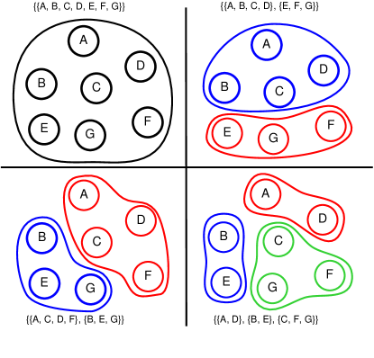
Figure 7: Partitions of tasks, equivalent to processor allocations.

Lemma 1.

The allocation phase of the AO model can produce all possible partitioning of tasks and there is only one unique sequence that produces each possible paritition.

Proof.

We show how any given allocation $A_{\Omega}$, which is a complete partition of $V$, is constructed with the proposed allocation procedure and that there is only one possible choice at each step. We begin with an empty partial allocation $A=\{\}$, and are presented with the tasks in $V$ in a fixed order $n_{1}$, $n_{2}$, … $n_{|V|}$. We must always begin by placing $n_{1}$ into a new part, so that $A=\{\{n_{1}\}\}$. Now we must place $n_{2}$. If $n_{1}$ and $n_{2}$ belong to the same part in $A_{\Omega}$, they must also be placed in the same part in $A$, and so we must have $A=\{\{n_{1},n_{2}\}\}.$ Conversely, if $n_{1}$ and $n_{2}$ belong to different parts in $A_{\Omega}$, the same must be true in $A$, and we make $A=\{\{n_{1}\},\{n_{2}\}\}.$ For each subsequent task $n_{i}$, if $n_{i}$ in $A_{\Omega}$ belongs to the same part as any of tasks $n_{1}$ to $n_{i-1}$, we must place it in the same part in $A$. If $n_{i}$ does not share a part in $A_{\Omega}$ with any task $n_{1}$ to $n_{i-1}$, it must be placed in a new part by itself. At each step, there is exactly one possible move that can be taken in order to keep $A$ consistent with $A_{\Omega}$. Since there is always at least one move, it is possible to produce any partition of $V$ in this fashion, and because there is always at most one move, there is only one path that will produce a given partition. Since each distinct allocation can only be produced with one unique sequence of moves, duplicate allocations are not possible. ∎

By Lemma 1, we have removed the first source of duplicates: there is no possibility of producing allocations that differ from each other only by the permutation of processors.

In a naive approach to allocation, in which we simply assign each task in $V$ to an arbitrary processor in $P$ without considering their homogeneity, there are $|P|^{|V|}$ possible outcomes. The number of possible complete allocations in this state space is given by the formula $\sum_{k=1}^{|P|}\begin{Bmatrix}|V|\\ k\end{Bmatrix}$, where $\begin{Bmatrix}n\\ k\end{Bmatrix}$ represents the number of distinct ways to divide a set of size $n$ into $k$ subsets (this being known as a Stirling number of the second kind) [30]. In the worst case, where the number of available processors is equal to the number of tasks, the formula gives us what is known as a Bell number: the total number of possible partitions of a set with size $n$. Bell numbers are known to be asymptotically bounded such that $B_{n}<(\frac{0.792n}{ln(n+1)})^{n}$[31]. This bound demonstrates that, although the number of allocations still grows exponentially, it is an exponential function of significantly lower order than the naive $|P|^{|V|}$approach.

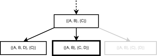
Figure 8: Branching in the allocation state-space with a maximum of two processors.

$A_{s}$ is a partial partition of $V$

function expand-alloc-state($s$, $V$, $|P|$)

     $unallocated\leftarrow V\setminus\bigcup\nolimits_{a\in A_{s}}a$

     $nextTask\leftarrow min_{n\in unallocated}topo\mathchar 45\relax order(n,G)$

     $children_{s}\leftarrow\emptyset$

     for all $a\in A_{s}$ do

         $s_{c}hild\leftarrow$ a copy of $s$

         $a_{c}hild\leftarrow$ the set in $A_{c}hild$ which is equal to $a$

         $a_{c}hild\leftarrow a_{c}hild\cup\{nextTask\}$

         $children_{s}\leftarrow children_{s}\cup\{s_{c}hild\}$

     end for

     if $\lvert A_{s}\rvert<|P|$ then

         $s_{c}hild\leftarrow$ a copy of $s$

         $a_{n}ew\leftarrow\{nextTask\}$

         $A_{c}hild\leftarrow A_{c}hild\cup\{a_{n}ew\}$

         $children_{s}\leftarrow children_{s}\cup\{s_{c}hild\}$

     end ifreturn $children_{s}$

end function

Algorithm 1 Defining children of an allocation state.

4.1.1 Allocation Cost Function

For branch-and-bound search using our AO state-space model to be effective, we need an admissable heuristic to determine our cost function $f$, such that $f(s)$ gives a lower bound for the minimum length of any schedule resulting from the partial partition $A$ at state $s$. The efficiency of a branch-and-bound search can be defined by the number of states in the state-space that need to be examined before a provably optimal solution can be found [32]. To prove that a solution is optimal, all states in the state-space with a lower $f$-value must be examined and shown to not be solutions themselves. Such states are said to be ’critical’ [33]. A tighter bound can make the search more efficient, while a looser bound may make the search less efficient. This is because a tighter bound is likely to increase the $f$-value of some states, possibly making them no longer critical, while a looser bound can do the opposite.

In the case of allocation, there are two crucial types of information we can obtain from a partial partition $A$, which allow us to determine a lower bound for the length of a resulting schedule. The first, and simplest, is how well the computational load is balanced between the different groupings of tasks. In an ideal case, with no gaps in execution, a processor assigned a grouping $a\in A$ will still require time equal to the sum of the computational weights $w(n)$ of the tasks $n\in a$, i.e. $\sum_{n\in a}w(n)$, in order to finish. The overall schedule length is therefore bounded by the total weight of the most heavily loaded grouping in $A$. We improve this bound further by considering the time at which execution can start on each processor. The earliest possible start time for a task $n$ is given by its allocated top level $tl_{\alpha}(n)$. The earliest that a processor can begin executing tasks can therefore be determined by finding the minimum allocated top level among its assigned tasks $n\in a$. Similarly, the minimum bottom level (disregarding the weight of the first task in the level path) among the grouping tells us the minimum amount of time required to reach the end of the schedule once all tasks on this processor have finished execution. We therefore add the minimum allocated top level and minimum bottom level (disregarding (disregarding the weight of first task in the level path) to each grouping’s computational load to obtain our first bound.

$$f_{l\mathrm{oad}}(s)=\mathrm{max}{}_{a\in A} \biggl{\{}min_{n\in a}tl_{\alpha}(n)+\sum_{n\in a}w(n)$$

$$+min_{n\in a}(bl_{\alpha}(n)-w(n))\biggr{\}}$$ (1)

The second bound derives from our knowledge of which communication costs must be incurred, and is obtained from the length of the allocated critical path of the task graph; that is, the longest path through the task graph given the particular set of allocations. It is usual when finding a critical path for a task graph to ignore the edge weights, as in an ideal case no communication costs would need to be incurred. However, if two tasks $i,j\in V$ have been assigned to different groupings in $A$, and an edge $e_{ij}$ exists between them, we now know that the communication represented by that edge must take place. Such edges can therefore be included when determining the critical path, and may increase its length. As all computations and communications in the allocated critical path must be completed in sequence, the overall schedule must be at least as long, and this gives us our second bound. Figure 9 shows an example of an allocated critical path. In practise, it is helpful to consider the allocated top and bottom levels of the tasks when determining the allocated critical path, since we use those values for several other calculations. The length of the longest path in a task graph which includes a task $n$ can be found by adding the top and bottom levels of $n$. It follows that the length of the allocated critical path is the greatest value for $tl_{\alpha}(n)+bl_{\alpha}(n)$ among all $n\in V^{\prime}$.

$$f_{\mathrm{acp}}(s)=\mathrm{max}_{n\in V^{\prime}}\left\{tl_{\mathrm{\alpha}}(n)+bl_{\alpha}(n)\right\}$$ (2)

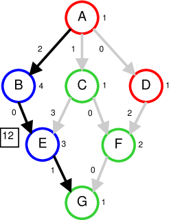
Figure 9: The allocated critical path heuristic.

Since we want the tightest bound possible, the maximum of these two bounds is taken as the final $f$-value.

$$f_{\mathrm{alloc}}(s)=\mathrm{max}\{f_{\mathrm{load}}(s),f_{\mathrm{acp}}(s)\}$$ (3)

By their nature, these two bounds oppose each other; lowering one is likely to increase the other. The shortest possible allocated critical path can be trivially obtained simply by allocating all tasks to the same processor, but this will cause the total computational weight of that processor to be the maximum possible. Likewise, the lowest possible computational weight on a single processor can be achieved simply by allocating each task to a different processor, but this means that all communication costs will be incurred and therefore the allocated critical path will be the longest possible. Combining these two bounds guides the search to find the best possible compromise between computational load-balancing and the elimination of communication costs.

4.2 Ordering

In the ordering phase, we begin with a complete allocation, and our aim is to produce a complete schedule $S$. After giving an arbitrary ordering to both the sets in $A$ and the processors in $P$, we can define the processor allocation in $S$ such that $n\in a_{i}\implies proc(n)=p_{i}$. The remaining step is to determine the optimal start time for each task. Given a particular ordering of the tasks $n\in p_{i}$, the best start time for each task is trivial to obtain, as it is simply the earliest it is possible for that task to start, considering the availability of the processor and the precedence constraints induced by the incoming edges. To complete our schedule we therefore only need to determine an ordering for each set of tasks $a_{i}\in A$. Our search could proceed by enumerating all possible permutations of the tasks within their processors. However, it is likely that many of the possible permutations do not describe a valid schedule. This will occur if any task is placed in order after one of its descendants (or before one of its ancestors).

In order to produce only valid orderings, an approach inspired by list scheduling is taken. In this variant, however, each processor $p_{i}$ is considered separately, with a local ready list $R(p_{i})$. Initially, a task $n\in p_{i}$ is said to be locally ready if it has no predecessors also on $p_{i}$. At each step we can select a task $n\in R(p_{i})$ and place it next in order on $p_{i}$. Those tasks which have been selected and placed in order are called ordered, while those which have not are called unordered. A simple definition of the local ready list states that a task $n\in p_{i}$ belongs to $R(p_{i})$ if it has no unordered predecessors also on $p_{i}$. Unfortunately, this formulation allows invalid states to be reached by the search, as seemingly valid local orders may combine to produce a schedule with an invalid global ordering. The simple definition still guarantees that all valid schedules can be produced, and invalid branches of the state-space can easily be removed from consideration: the f-value of certain invalid states is undefined, and in calculcation will increase indefinitely. However, an indeterminate amount of work may be wasted in exploring these invalid states. A correct formulation of the local ready list requires that any task $n_{i}$ which is ordered on $p_{i}$ must be subsequently considered to be a predecessor of any task $n_{j}$ on $p_{i}$ which is still unordered. This more complex ready condition is explained in detail in Section 5.

After a task $n$ has been ordered, each of its descendants on $p_{i}$ must be checked to see if the ready condition has now been met, in which case they will be added to $R(p_{i})$. Following this process to the end, we can produce any possible valid ordering of the tasks on $p_{i}$. Figure 10 illustrates a single state in an ordering state-space, and shows the options for branching which are available. In this example, several tasks have already been ordered on processor $P1$, and it has again been selected for consideration. Since they have no unordered predecessors also on $P1$, tasks $e$ and $f$ are both ready to be ordered. There are therefore two possible children of this state, one in which each of these ready tasks is placed next in order on $P1$. Note that $f$ is ready to be ordered despite the fact that its parent, $d$, has not been ordered. Since $d$ is allocated to a different processor, it is not considered when determining the readiness of $f$. Neither is its own parent, $a$, which would necessarily have been the very first task scheduled under the ELS model.

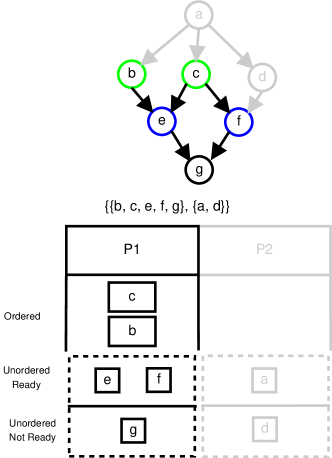
Figure 10: A single state in the ordering state space.

Producing a full schedule requires that this process be completed for all processors in $P$. At each level of the search, we can select a processor $p_{i}\in P$ and order one of its tasks. The order in which processors are selected can be decided arbitrarily; however, in order to avoid duplication, it must be fixed by some scheme such that the processor selected can be determined solely by the depth of the current state. The simplest method to achieve this is to proceed through the processors in order: first order all the tasks on $p_{1}$, then all the tasks on $p_{2}$, and so on to $p_{n}$. Another method is to alternate between the processors in a round-robin fashion. Unlike in exhaustive list scheduling, tasks are not guaranteed to be placed into the schedule in topological order. When a task is ordered, its predecessors on other processors may still be unordered, and therefore their start times may not be known. During the ordering process, therefore, a task $n$ may only be given an estimated earliest start time $eest(n)$. For all unordered tasks, $eest(n)=tl_{\mathrm{\alpha}}(n)$, its allocated top level. For ordered tasks, we first define $prev(n)$ as the task ordered immediately before $n$ on the same processor $proc(n)$. We also define the estimated data ready time $edrt(n_{j})=max_{n_{i}\in parents(n_{j})}\left\{eest(n_{i})+w(n_{i})+c(e_{ij})\right\}$. Where $prev(n)$ does not exist, $eest(n)=edrt(n)$. Otherwise, $eest(n)=max(eest(prev(n))+w(prev(n)),edrt(n))$. These are the same as the conditions for determining the earliest start time of a task in ELS whose ancestors have already been scheduled, but replacing the fixed, known start times of these ancestors with estimated earliest start times in each instance.

In our implementation, the changes in estimated earliest start times caused by the ordering of each new task $n_{\Delta}$ are propagated recursively. First, $eest(n_{\Delta})$ is calculated based on the EEST of the parents of $n_{\Delta}$, and the EEST of the task immediately preceding it on its processor $proc(n_{\Delta})$. The algorithm then proceeds to update the EEST of all ordered tasks whose start times depend on $n_{\Delta}$ - any of its children which, being allocated to a different processor, may have already been ordered. Once the EEST of all these tasks has been recalculated, we continue propagating to any previously ordered tasks which depend on them, and so on. In this case, dependent tasks include not only children, but also tasks which may be scheduled immediately after them on their respective processor. The red arrows in figure 11 show how the EEST updates are propogated after the ordering of task $a$, both through the original communication dependencies in the task graph and the new dependencies determined by the previously decided ordering.

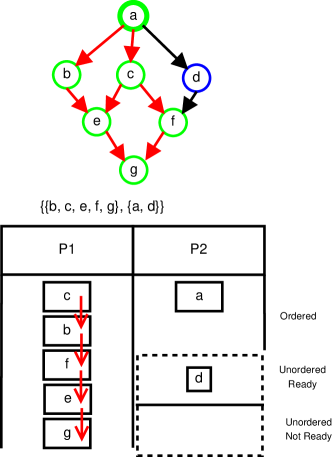
Figure 11: Updating estimated earliest start times after ordering a new task.

In this way, we have solved the problem of duplicates arising from making the same decisions in a different order. By allocating each task to a processor ahead of time, and enforcing a strict order on the processors, it is no longer possible for these situations to arise. Where before we might have placed task $n_{2}$ on $p_{2}$ and then task $n_{1}$ on $p_{1}$, we now must always place task $n_{1}$ on $p_{1}$ and then task $n_{2}$ on $p_{2}$.

Lemma 2.

The ordering phase of the AO model can produce all possible valid orderings of tasks and there is only one unique sequence that produces each possible ordering.

Proof.

This proof is similar to that of Lemma 1. We show how any given complete valid schedule $S_{\Omega}$, which implies the complete allocation $A_{x}$, is constructed with the proposed ordering procedure and that there is only one possible choice at each step. Consider the sequence of moves required to replicate $S_{\Omega}$. We begin with an empty schedule $S$, and then select processors for consideration in a fixed and deterministic order (e.g. round robin). Say that we select $p_{i}$. In schedule $S_{\Omega}$, there is a task $n_{x}$ which is next in order on $p_{i}$. Since $S_{\Omega}$ is a valid schedule consistent with $A_{x}$, $n_{x}$ must belong to the current ready queue for $p_{i}$. Since $n_{x}$ is next in order in $S_{\Omega}$, it must be selected to be ordered next in $S$. At each step, there is exactly one possible move that can be taken in order to keep $S$ consistent with $S_{\Omega}$. Since there is always at least one move, it is possible to produce any schedule consistent with $A_{x}$ in this fashion, and because there is always at most one move, there is only one path that will produce a given schedule. Since each distinct schedule can only be produced with one unique sequence of moves, duplicate schedules are not possible. ∎

Please note that this lemma is not ruling out the creation of invalid orderings. How they are avoided is discussed in 5.

Ordering Cost Function

The heuristic for determining $f$-values in the ordering stage follows a similar pattern to that for allocation. The difference lies in the fact that independent tasks allocated to the same processor can now delay one another. During the allocation phase, our critical path heuristic assumes that every task begins as early as it theoretically could on the processor it is assigned to, only based on the allocated top-level. Another way of looking at this is that we assume that every task will be first in order (and that this is also true for all ancestors). Clearly this is not the case, and as we decide the actual order of the tasks on a processor $p$, the tasks which are placed earlier in the order are likely to push back the start times of the tasks placed later in the order, as they must wait to be executed. Communications from other processors can also introduce idle times, during which the processor does nothing as the data required for the task next in order is not yet ready. The $eest$ of a task takes both of these factors into account. For each state $s$, the current estimated finish time of a processor $p_{i}$ is the latest estimated finish time of any task $n\in V:proc(n)=p_{i}$ which has so far been ordered. This estimated finish time must include both the full computation time of each task already ordered on $p_{i}$, as well as any idle time incurred between tasks.

With this in mind, we define our two bounds like so: first, the latest estimated start time of any task already ordered, plus the allocated bottom level of that task. We refer to this as the partially scheduled critical path, as it corresponds to the allocated critical path through our task graph, but with the addition of the now known idle times and intra-processor communication delays.

$$f_{\mathrm{scp}}(s)=\mathrm{max}_{n\in ordered(s)}\left\{eest(n)+bl_{\mathrm{\alpha}}(n)\right\}$$ (4)

Second, the latest finish time of any processor in the partial schedule, plus the total computational weight of all tasks allocated to that processor which are not yet scheduled.

$$f_{\mathrm{ordered-load}}(s)=\mathrm{max}{}_{p\in P}\left\{t_{\mathrm{f}}(p)+\sum_{n\in p\cap unordered(s)}w(n)\right\}$$ (5)

Again, this corresponds to the total computational load on a processor with the addition of now known idle times and intra-processor delays. To obtain the tightest possible bound, the maximum of these bounds is taken as the final $f$-value.

$$f_{\mathrm{order}}(s)=\mathrm{max}\{f_{\mathrm{scp}}(s),f_{\mathrm{ordered-load}}(s)\}$$ (6)

4.3 Combined State-Space

Solving a task scheduling problem instance requires both the allocation and ordering sub-problems to be solved in conjunction. To produce a combined state-space, we begin with the allocation search tree, $S_{\mathrm{A}}$. The leaves of this tree represent every possible distinct allocation of tasks in $G$ to processors in $P$. Say that leaf $l_{i}$ represents allocation $A_{i}$. We produce the ordering search tree $S_{\mathrm{O}_{i}}$ using $A_{i}$. The leaves of $S_{\mathrm{O}_{i}}$ represent every distinct complete schedule of $G$ which is consistent with $A_{i}$. If we take each leaf $l_{i}$ in $S_{A}$ and set the root of tree $S_{\mathrm{O}_{i}}$ as its child, the result is the combined tree $S_{\mathrm{AO}}$, the leaves of which represent every distinct complete schedule of $G$ on the processors in $P$. Figure 12 demonstrates how all of the ordering sub-trees in $S_{AO}$ sprout from the leaves of the allocation tree above them.

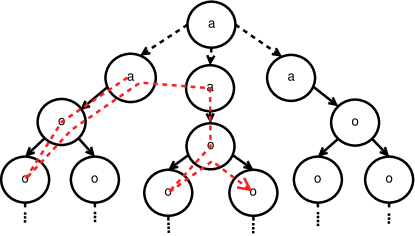
Figure 12: A possible search path through the combined state space.

A branch-and-bound search conducted on this state-space will begin by searching the allocation state-space. Each allocation state representing a complete allocation has one child state, which is an initial ordering state with this allocation. When considering the allocation sub-problem in isolation, we define the optimal allocation as that which has the smallest possible lower bound on the length of a schedule resulting from it. Unfortunately, these lower bounds cannot be tight and therefore it is not guaranteed that the allocation with the smallest lower bound will actually produce the shortest possible schedule. This means generally that in the combined state-space, a number of complete allocations are investigated by the search and have their possible orderings evaluated, as represented by the red arrow in figure 12. The tighter the bound which can be calculated, the more quickly the search is likely to be guided toward a truly optimal allocation.

5 Avoiding Invalid States

The simple definition of a ready list as done in Section 4.2 enforces valid local orders for all processors, but in same cases their combination can be an invalid global ordering. To explain why this happens, we model a partial schedule as a graph showing all of the dependencies between tasks. For a task graph $G$, a partial schedule $S^{\prime}$can be represented by augmenting $G$ to produce a partial schedule graph $G_{S^{\prime}}.$ We begin with the graph $G$. Say that in $S^{\prime}$, a task $n_{1}$ is ordered on processor $p_{1}$, and a task $n_{2}$ is also ordered on $p_{1}$, but later in the sequence. We check for the edge $e_{12}$ in the task graph. If $e_{12}\notin E$, we add $e_{12}$to $E$. This new edge represents that, according to the ordering defined by our partial schedule, $n_{2}$must begin after $n_{1}$. This can be considered as a new type of dependency, which we call an ordering dependency, as opposed to the original communication dependencies in $G$. Once edges have been added corresponding to all ordered tasks in $S^{\prime}$, we have our graph $G_{S^{\prime}}$. The presence of a cycle in this graph indicates that the ordering is invalid, as a cycle of dependencies is unsatisfiable. Since the graph $G$ is acyclic, and if $n_{i}$ is an ancestor of $n_{j}$ in $G$ then the ordering edge $e_{ji}$ cannot be created, it is necessary that any cycle in $G_{S^{\prime}}$ will contain at least two ordering edges. Figure 13 shows a minimal example of such a cycle, with ordering edges marked by dashed lines.

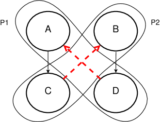
(a) Task graph and allocation.

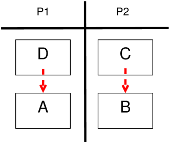
(b) Ordering which produces a cycle.

Figure 13: A minimal example of a cycle created by ordering edges.

In our preliminary work in [9], such states were removed from consideration during the search as their cyclic nature made their $f$-values increase infinitely during calculation, until they passed an upper bound for the schedule length and it was clear they could be ignored. However, it is possible for a state to exist in which no cycle yet exists, but for which it is inevitable that a cycle will be created as the ordering process continues. Say, for example, that the introduction of edge $e_{ij}$ would create a cycle in $G_{S^{\prime}}$, but in $S^{\prime}$ the task $n_{i}$ has already been ordered while $n_{j}$ has not. In order for the schedule to be completed, $n_{j}$ must eventually be ordered, at which point a cycle will be formed. Here, $S^{\prime}$represents an entire subtree of states from which no valid schedule can be reached. None of these states can be selected as the optimal solution, so this does not present a threat to the accuracy of the search process. However, it does represent a potentially substantial amount of wasted work performed by the search algorithm. Ideally the formulation of the AO model would be such that it allows the creation of any valid solution, and only valid solutions.

The key to avoiding this unnecessary work is the observation that, given that $n_{i}$ has been ordered and $n_{j}$ has not, it is inevitable that $n_{j}$must eventually be ordered later than $n_{i}$. Therefore, for all descendents of this partial schedule in which $n_{j}$ is ordered, the ordering edge $e_{ij}$ must be in $G_{S^{\prime}}$. We can therefore define a more useful augmented task graph, $G_{S^{\prime}}^{*}$, which ’looks ahead’ to determine cycles that must inevitably occur. In this graph, the ordering edge $e_{ij}$ exists if $proc(n_{i})=proc(n_{j})$ and either $n_{j}$ is ordered later than $n_{i}$, or $n_{i}$ has been ordered and $n_{j}$ has not.

To avoid these cycles, we propose a modification to the condition we use to determine if a task is free to be ordered. The new condition is this: a task $n_{i}$ on processor $p_{i}$ is free to be ordered if it has no ancestors in graph $G_{S^{\prime}}^{*}$ which are also on $p_{i}$ and have not already been ordered in $S^{\prime}$. In the original formulation of AO, this condition used only the graph $G$. However, the ordering edges specific to the partial solution $S^{\prime}$ must be considered equally with the communication edges that are common to all partial solutions. The creation of a cycle in $G_{S^{\prime}}^{*}$ requires that an ordering edge is introduced from a task $n_{i}$ to task $n_{j}$, where $n_{i}$ was already reachable from $n_{j}$ using at least one ordering edge. By definition, this means that $n_{j}$ is the ancestor of $n_{i}$ in $G_{S^{\prime}}^{*}$. Therefore, according to the new condition, $n_{i}$ cannot be considered free until $n_{j}$ has been ordered, meaning that the edge $e_{ij}$ can never be introduced and the cycle can never be formed. By treating the ordering dependencies created during the ordering process in the same way as the original communication dependencies, we ensure that states with an invalid global ordering cannot be reached.

We implement this more precise definition of a free task by maintaining a record of $G_{S^{\prime}}^{*}$with each state in the form of a transitive closure matrix. Whenever a new task is ordered, the transitive closure is updated to reflect the new ordering dependencies. We can then use this matrix to determine which tasks are free when creating the children of a state.

5.1 Evaluation

Use of the simpler definition of the ready list as in Section 4.2 does not produce incorrect results; invalid states eventually have their f-values escalate indefinitely, and hence are quickly removed from consideration. An indeterminate amount of work was wasted before reaching and removing these obviously wrong states, however. We therefore find it necessary to evaluate whether the work saved by avoiding invalid states outweighs the additional algorithmic overhead necessary to do so. To determine experimentally the impact of this, we performed A* searches on a set of task graphs using versions of the model both with invalid state avoidance and without. Task graphs were chosen corresponding to a wide variety of program structures. Approximately 270 graphs with 21 tasks were selected. These graphs were a mix of the following DAG structure types: Independent, Fork, Join, Fork-Join, Out-Tree, In-Tree, Pipeline, Random, Series-Parallel, and Stencil. We attempted to find an optimal schedule using both 2 and 4 processors, once each for both versions of AO, giving a total of over 1000 trials. All tests were run on a Linux machine with 4 Intel Xeon E7-4830 v3 @2.1GHz processors. The tests were single-threaded, so they would only have gained marginal benefit from the multi-core system. The tests were allowed a time limit of 2 minutes to complete. For all tests, the JVM was given a maximum heap size of 96 GB.A new JVM instance was started for every search, to minimise the possibility of previous searches influencing the performance of later searches due to garbage collection and JIT compilation.

Figure 14 shows the results of these tests. We use a form of plot know as a performance profile: the $x$-axis shows time elapsed, while the $y$-axis shows the cumulative percentage of problem instances which were successfully solved by this time. Both versions of AO were able to solve approximately 70% of the problem instances within 2 minutes, with a slight advantage for invalid state avoidance. This suggests that the presence of invalid states does not have too much of a negative impact on average. It also suggests, however, that the addition of the transitive closure and associated operations does not significantly slow down the implementation of the AO formulation.

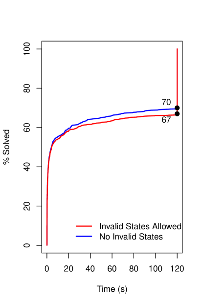
Figure 14: Comparing the performance of AO with and without invalid states.

6 Pruning Techniques and Optimisations

Now that the novel AO model and the search through its solution space have been proposed, it is important to investigate pruning techniques and other optimisations which can be used with it. A search of the AO state-space model is theoretically able to benefit from several pruning techniques and optimisations already developed for ELS. Namely, these are identical task pruning, fixed order pruning and a heuristic upper bound [12, 8]. We discuss them in the following, see which have become obsolete and then propose a new additional pruning technique.

6.1 Adapted from ELS

Identical Task

Two tasks $A$ and $B$ are considered identical if they are indistinguishable from each other in any way except by their name [34]. This means they have the same weight, same children, same parents, and same communication costs to and from those respectively. If tasks are identical, then their positions in any schedule can be freely swapped without any effect on the rest of the schedule. Therefore, the relative ordering of a set of such tasks, $I$, does not matter. We only need to consider one such order for our search.

To do this in ELS, we augment the task graph by creating a chain of “virtual edges” linking tasks in $I$. A virtual edge from task $A$ to task $B$ prevents $B$ from being considered for scheduling before $A$, but does not imply any other dependency. It has no weight, and $A$ does not have to finish before $B$ can be started. Virtual edges, therefore, only have an impact on deciding which tasks belong to the current ready list. $B$ cannot be added to the ready list until $A$ is scheduled. In this way it is ensured that only one order for the identical tasks in $I$ is allowed.

In AO, this pruning can also be applied, but we need to distinguish the allocation (A) and the ordering (O) phase. In the allocation phase we take advantage of identical tasks to provide additional pruning . Not only does the ordering of identical tasks not matter, a task $A$ on processor $p_{1}$ can be swapped with its identical task $B$ on $p_{2}$ without consequence. The processor that an individual task in a set of identical tasks is allocated to does not matter. What matters, therefore, is what number of the tasks in $I$ belong to each part of the allocation. While building our allocation, we give the parts of the allocation an arbitrary index order. Say that part $a_{x}\in A$ is the part with highest index to which any task in $I$ is allocated. When a task $n_{i}\in I$ is next to be allocated, we restrict the parts to which it may be assigned to only those $a_{i}\in A|i\geq x$. Essentially, as we allocate the tasks in $I$, we first decide how many of the identical tasks are assigned to $a_{0}$, then how many are assigned to $a_{1}$, and so on. In this way, we avoid producing any allocations which differ only in the permutation of identical tasks across processors.

During the ordering phase the pruning technique is applied in much the same way as in ELS. However, since we consider only local ready lists, the virtual edges are not always relevant. If identical tasks $A$ and $B$ are allocated to the same processor, then the virtual edge from $A$ to $B$ will be respected, and only orderings in which $A$ goes before $B$ will be produced. If $A$ and $B$ are on different processors, however, then the order in which they are considered for scheduling is instead decided by the order in which processors are considered. These virtual edges will therefore be ignored.

Heuristic Upper Bound

A solution to a task scheduling problem can be found quickly (that is, in polynomial time) using a heuristic algorithm. The length of an approximate solution can then be used as an upper bound for f-values in an optimal search. Since we have an example of a solution with this length, it is guaranteed that no solution with a higher f-value can be optimal. The A* algorithm will not examine states with higher f-values than the optimal solution, so this optimisation will not prevent additional states from being created. However, it can save memory as states that will never need to be examined do not need to be stored. Additionally, if the heuristic happens to find an optimal solution, it saves us from searching through an indeterminate number of equal f-value states. As soon as our best state has that f-value, we know we can stop and take the heuristic solution - now proven to be optimal [34, 8].

The AO model is able to use this technique in just the same way as ELS, with no special consideration required.

Fixed Task Order

For a fork graph, it is guaranteed that an optimal schedule exists in which the tasks are scheduled in order of non-decreasing in-edge weight [12]. Given such an order for the tasks, all that is required to find the optimal schedule is a search for an optimal allocation of tasks. Conversely, for join graphs, the same is true if the tasks are scheduled in order of non-increasing out-edge weight. In a fork-join graph, if an order can be found which satisfies both the fork and the join condition simultaneously, then this order is also optimal. We can therefore fix the order of this set of tasks, eliminating the need to search all permutations.

In fact in ELS, whenever the current set of ready tasks fulfills these conditions, their order can be fixed [12]. This fixed order can then be followed until changes to the ready list invalidate the fixed order conditions. This property allows the technique to be extended to graphs which are not purely independent, a fork, join, or fork-join, but merely contain these as a sub-structure. If in any state the current ready tasks all belong to such a sub-structure, it may be possible to fix their order. It also means that if a fork-join graph does not immediately meet the fixed order conditions, the conditions may still be met in subsequent states and allow the order to be fixed for certain sub-trees.

For AO, if we are able to fix the order of all the tasks in a graph then only the allocation phase of our search is relevant, and the ordering phase becomes trivial. Generally, in the ordering phase, we can apply our fixed order conditions to the tasks in a local ready list. If the conditions hold for the currently ready tasks on a given processor, then the local order of these tasks can be fixed. Since these local ready lists are smaller than the global ready list of ELS, they are less likely to contain a task which contradicts the fixed order conditions. Additionally, the number of chances for an order to be fixed increases by a factor of $|P|$. It is therefore probable that the order of tasks can be fixed more often when using AO, albeit for smaller sets of tasks. We can even fix the order of multiple fork-join substructures in a graph at the same time, as long as they are assigned to different processors.

6.2 Obsolete

Since there are no duplicates in the AO model, the pruning techniques used to mitigate the impact of duplicates in ELS [9]are no longer relevant.

Duplicate Detection

In ELS, there is no way to mitigate the effect of independent scheduling order duplicates (Section 2.3) except to keep a record of all states found so far. Binary search trees are used to store both an open set (containing states created but not yet explored) and a closed set (containing states which have already been expanded) [8]. Each time a state is created, it must be ensured that neither the open nor the closed set already contain this state. If they do, then this state is a duplicate and is discarded. The need for the closed set means that all states created must be kept in memory for the duration of the search. The time taken to search the open and closed sets is $O(lg(k))$, where $k$ is the number of states so far created by the search.

Since there are no duplicates in AO, it is not necessary to maintain a closed list. It is also unnecessary to compare new states against the open list, which permits the use of more efficient data structures for the open list. AO therefore has a very large advantage in terms of memory usage, and a small but perhaps practically significant advantage in time complexity.

Processor Normalisation

In order to avoid processor permutation duplicates (Section 2.3) in ELS, each state created has its partial schedule $S^{\prime}$ transformed into a normalised form $S_{N}^{\prime}$ [8]. In the ELS implementation compared here, we rename and therefore ’re-order’ the processors to which tasks are assigned in $S^{\prime}$, in a way that ensures that all processor permutation duplicates of $S^{\prime}$ are transformed to the same normalised form. First, we give a total ordering to the tasks in $V$. This can be any order, so long as it is used consistently, but is likely to be the same topological order used elsewhere. We can then define $min(p_{i})$ as the task $n$ with lowest value among those assigned to $p_{i}$. The ordering of processors is then defined such that $min(p_{i})<min(p_{j})\implies p_{i}<p_{j}$. Once the processors are re-ordered according to this scheme, we have our normalised partial schedule $S_{N}^{\prime}$. By normalising all states in this way, we can use the previously discussed duplicate detection mechanism in order to remove processor permutation duplicates from consideration.

The method used by the AO model for its allocation phase makes this process unnecessary, as it simply does not allow these duplicates to be produced in the first place. In essence, the method of iteratively building a partition from an ordered list of tasks ensures that each state produced is automatically in its normalised form. In other words, if the processor normalisation process were to be applied to one of AO’s partial allocations no re-ordering would ever take place, as the processors are in their normalised order at all times.

6.3 Novel

Graph Reversal

Among the standard task graph structures, there are several pairs which differ only by the direction of their edges. Most obviously, reversing the edges of a fork graph produces a join graph, and vice versa. It can also be observed that, for both the ELS and AO models, join graphs are significantly more difficult to solve than fork graphs, as evident in Figure 16. This arises from the fact that in both models tasks are allocated to processors in a topological order. In a fork graph, all communications originate from the source task. Being a source, and therefore first in topological order, this task is always the first to be allocated, and from that point on it will always be known whether a communication cost is incurred or not as soon as the other corresponding task is allocated. Conversely, in a join graph, all communications go to the sink task. Since it is last in topological order, all other tasks are allocated before it without any knowledge of which communications are incurred. The decision of which communication costs to set to zero is made all at once, in the last step. Since knowledge about communication costs is critical to determining a lower bound on the eventual length of a partial schedule, it is clear to see why fork graphs, where this information is always available, can be solved much more efficiently than join graphs, where this information is not available until too late.

We define $R(G)$, the reverse of a task graph $G$, simple by reversing the direction of each edge $e\in G$. If we do this for a join graph, the result is a corresponding fork graph. We can then find an optimal schedule $S_{R(G)}^{*}$ for this reversed graph. If this reversed graph is now a fork, it can be solved much more efficiently than the original join. Our optimal schedule for $R(G)$ can then be reversed to obtain a valid schedule for $G$. Reversing a schedule simply means reversing the ordering of the tasks allocated to each processor, so that the task scheduled first is now scheduled last, and so on. Using, this ordering, each task is started as early as possible, subject to the processor availability and precedence constraints. This reversed schedule $R(S_{R(G)}^{*})$ is now an optimal schedule $S_{G}^{*}$ for the original graph. This known result is easy to show. Taking a schedule and reversing its time line, while at the same time reversing the direction of all edges results in a valid schedule for the reversed graph. The reversed schedule and the original must have the same length - the same computation and communication delays occur, only in backwards order. In the reversed schedule, not all tasks might start at their earlist possible time, but rescheduling them earlier has no negative impact on the schedule length (this is done automatically in the above described procedure as we only take the order of the tasks). If a shorter schedule for $G$ existed, it could in turn be reversed to produce a shorter valid schedule for $R(G)$, and so $S_{R(G)}^{*}$ could not have been an optimal schedule in the first place. Instead of solving difficult join graphs, we can instead transform them into fork graphs, solve these much more easily, and then transform the resulting schedules to produce optimal schedules for the original joins. This technique is also applied to out-tree and in-tree graphs, of which fork and join are special cases, respectively.

7 Evaluation

In this section we evaluate the benefit of the new AO state-space model in the search for optimal solutions. For this purpose it is compared against the use of the ELS model. The empirical evaluation was performed by running branch-and-bound searches on a diverse set of task graphs using each state-space model. Task graphs were chosen that differed by the following attributes: graph structure, the number of tasks, and the communication-to-computation ratio (CCR). Table LABEL:tab:Range-of-task describes the range of attributes in the data set. A set of 1360 task graphs with unique combinations of these attributes were selected. These graphs were divided into four groups according to the number of tasks they contained: either 10 tasks, 16 tasks, 21 tasks, or 30 tasks. An optimal schedule was attempted for each task graph using 2, 4, and 8 processors, once each for each state-space model. This made a total of 4080 problem instances attempted per model. Searches were performed using the A* search algorithm. All pruning techniques discussed in the previous section were applied to each state-space model that could take advantage of them.

Graph Structure

• Independent

• Fork

• Join

• Fork-Join

• Out-Tree

• In-Tree

• Pipeline

• Random

• Series-Parallel

No. of Tasks

• 10

• 16

• 21

• 30

CCR

• 0.1

• 1

• 10

Table 1: Range of task graphs in the experimental data set.

The implementations were built with the Java programming language. An existing implementation of ELS[12] was used as the basis for an AO implementation, with code for common procedures shared wherever possible. Notably, the basic implementation of the A* search algorithm is shared, with the implementations differing only by how the children of a search node are created. The implementations of commonly applicable pruning techniques are also shared. Using this approach, the differences observed in the experimental results are most like due to the different models and not implementation artifacts.

All tests were run on a Linux machine with 4 Intel Xeon E7-4830 v3 @2.1GHz processors. The tests were single-threaded, so they would only have gained marginal benefit from the multi-core system. The tests were allowed a time limit of 2 minutes to complete. For all tests, the JVM was given a maximum heap size of 96 GB. A new JVM instance was started for every search, to minimise the possibility of previous searches influencing the performance of later searches due to garbage collection and JIT compilation.

7.1 Results and discussion

For the 10-task group, every problem instance was solved within at most 3 seconds, regardless of the state-space model used. It is apparent that both models are powerful enough that task graphs this small will not present a challenge, and so we will not discuss these results further. The other three groups will be discussed in detail in the following.. Figure 15 shows performance profiles (as used in Section 5.1) that compare the performance of the two models, broken down by graph size. These charts indicate the accumulated percent of problem instances in the data set that were successfully solved after a given time had elapsed, up to the timeout of 120 seconds. In the 16 task group, a large majority of the problem instances were able to be solved by both models, but AO gives a clear advantage. By the timeout, 90% of instances were solved by AO, while only 77% were solved by ELS. In the 21 task group, we see an even more dramatic difference: while ELS solves only 46% of instances within two minutes, AO manages to solve 70%. Graphs of size 30 are difficult to solve within two minutes for both models. Although ELS is seen to have a slight advantage in the first few seconds of runtime, by the end of two minutes the lines have converged and both models solve 19% of instances. Overall, AO has significantly better performance in these experiments, particularly in the “medium difficulty” 21 task group. Not only does it solve more instances within a few seconds, the gap between the models widens as time goes on, with AO consistently solving more instances than ELS.

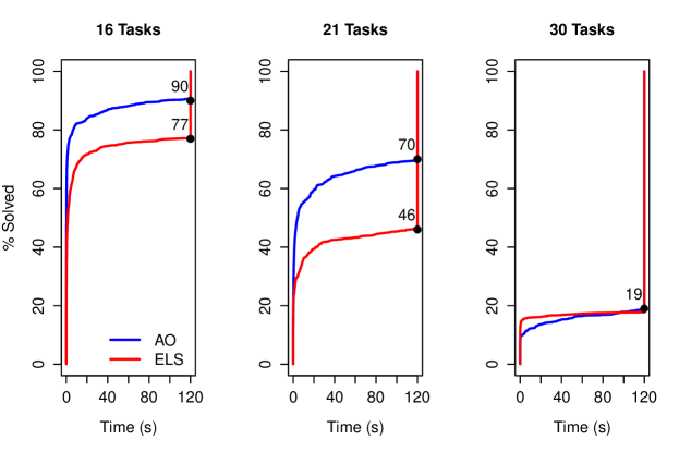
Figure 15: Overall performance of the two models.

Breaking the results down by graph structure, we see that AO has a clear advantage for most structures. Figure 16 shows the solved instances within the time limit by model in stacked bar charts across the different structures. In the 16 and 21 task graphs, AO dominates ELS in almost all structures. For 30 tasks, it is clear that graphs of this size present a significant challenge for both models, as a large majority of problem instances were not solved by either. Overall, both models solved 19% of graphs in this group. ELS shows better performance with Independent, Random, and Stencil graphs, while AO is better for the other structures. The large number of non-solved instances in this size category makes it difficult to draw further conclusions.

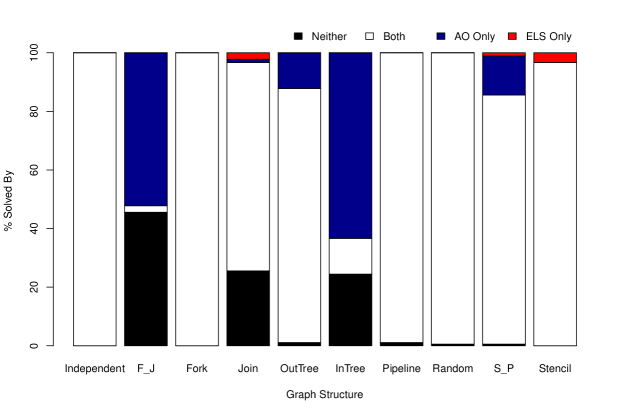
(a) 16 Tasks

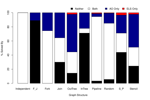
(b) 21 Tasks

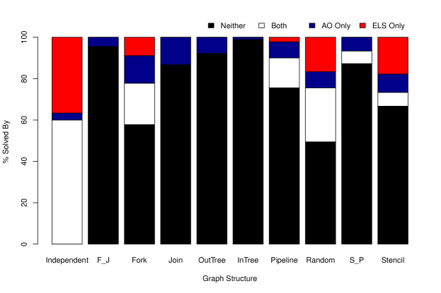
(c) 30 Tasks

Figure 16: Performance of the models broken down by graph structure.

Comparing by the communication-to-computation ratio of the task graphs (Figure 17), we see that AO has an advantage at all values, but is dramatically better at solving graphs with very high CCR of 10. By deciding the allocation of tasks first, a search using the AO model very quickly determines the entire set of communication costs which will be incurred. Allocations which incur very large communication costs are likely to be quickly ruled out, and knowledge of all the communication costs can be used in the calculation of $f$-values throughout the ordering stage. For graphs in which communication is dominant, it is intuitive that early knowledge of the communication would allow more efficient decision-making, and these results support that intuition.

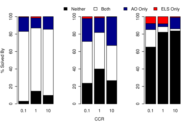
Figure 17: Performance of the models broken down by CCR.

The newly implemented reversed-join pruning technique allowed for a dramatic increase in the number of join and in-tree task graphs able to be solved, as seen in Figure 18, where the ’-R’ graph name extension indicates that the graph was reversed before scheduling. As would be expected, the performance trend for reversed join graphs is very similar to that for fork graphs, and the same is true for reversed in-tree and out-tree graphs. Both AO and ELS are able to solve many more graphs this way, but the impact is more significant for AO.

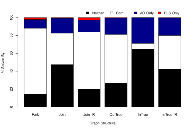
Figure 18: The effect of reversing Join and In-Tree task graphs.

8 Advanced Lower Bound Heuristics

Section 4 described intuitive and essential bounds and corresponding $f$-value functions to use for the initial implementation of the AO state space. However, it is likely that tighter bounds could improve the performance of searches using AO. Below we describe various improvements which allow these bounds to be tightened in some circumstances. These new bounds all apply to the Allocation phase of the state-space. Since this is the part of the model which is most distinct from ELS, it appears to offer the most new opportunities for heuristic development.

Minimum Finish Time

The allocation-load heuristic (Section 4.1.1,$f_{load}$(1)) was intended to provide an estimate for the finish time of each processor, using the trivial fact that a processor will require at least as much time as is necessary to execute all of its allocated tasks. The addition of the minimum allocated top and bottom levels was a simple step which acknowledged that processors must sometimes wait for data to be communicated to them before they can begin execution. However, it is also often the case that a processor cannot execute all of its tasks in one unbroken stretch, and additional idle time must occur. Idle time is time during the run of a schedule when a processor is not performing any computation. This is often necessitated when a processor has finished execution of one task but has not yet received all data necessary to begin the next task in order. It is required to wait while computation and communication associated with that task’s ancestors is performed by other components of the system. The time at which a processor receives all the necessary data for a task $n$ and may begin execution is known as the data-ready time, $drt(n)$. In any schedule, for a given task $n$, it must always be the case that $t_{s}(n)\geq drt(n)\geq tl_{\alpha}(n)$. It follows from this that we may obtain a tighter bound by considering the allocated top levels of all tasks on a processor, thereby including some additional idle time.

Consider a single grouping $a$ in a partial partition $A$. When scheduled, each task $n\in a$ will have some finish time $t_{f}(n)=t_{s}(n)+w(n)$. We wish to find a lower bound for the value $T_{F}(a)=max_{n\in a}\{t_{f}(n)\}$. A simple observation is that $T_{F}(a)\geq max_{n\in a}\{tl_{\alpha}(n)+w(n)\}$: the minimum finish time must be at least as large as the maximum of the earliest possible finish times of the tasks. However, in many cases a task $n$ will not be able to start at $tl_{\alpha}(n)$ without overlapping execution of tasks and violating the processor constraint. Execution of the final task must be delayed until all other tasks are completed.

Given a total ordering $O_{a}$ for the tasks $n\in a$, let task $n_{i}$ be the i^th in order according to $O_{a}$. The earliest possible starting time for task $n_{i}$ adhering to order $O_{a}$ is then $t_{est}(n_{i},O_{a})=max\{tl_{\alpha}(n_{i}),t_{est}(n_{i-1},O_{a})+w(n_{i-1})\}$, with $t_{est}(n_{0},O_{a})=tl_{\alpha}(n_{0})$. It follows for the order $O_{a}$ that $T_{F}(a,O_{a})\geq max_{n\in a}\{t_{est}(n,O_{a})+w(n)\}.$

To use this in a lower bound, we now need to find an ordering which minimises $T_{F}(a)$.

Lemma 3.

Let $O_{a}^{tl_{\alpha}}$ be the ordering of the tasks $n\in a$ in non-descending allocated top level order $tl_{\alpha}$. Then $T_{F}(a,O_{a}^{tl_{\alpha}})\leq T_{F}(a,O_{a})$ for all possible orders $O_{a}$ of tasks in $a$.

Proof.

The proof is by contradiction. Assume there is an ordering$O_{a}^{*}\neq O_{a}^{tl_{\alpha}}$ with $T_{F}(a,O_{a}^{tl_{\alpha}})>T_{F}(a,O_{a}^{*})$. Now consider two adjacent tasks $n_{j-1}$ and $n_{j}$, $1\leq j\leq|a|-1$, in the ordering $O_{a}^{*}$. If $tl_{\alpha}(n_{j})\geq tl_{\alpha}(n_{j-1})$, they are already in the same relative order as in $O_{a}^{tl_{\alpha}}$. Otherwise, their order can be swapped without increasing the earliest start time of the following tasks, $t_{est}(n_{i}),\forall i>j$. This is true because $tl_{\alpha}(n_{j})<tl_{\alpha}(n_{j-1}),$and so there is no gap (idle time) between the two tasks. This means they can be swapped and placed again without any gap, such that the now first task $n_{j}$ starts at the original $t_{est}(n_{j-1}O_{a}^{*})$. Following this, the now later task $n_{j-1}$ will finish at the original $t_{f}(n_{j},O_{a}^{*})$, and therefore the swap does not impact on the following tasks in the order. Repeatedly swapping all task pairs that are not in order until there is no such pair left, will then bring all tasks of $a$ into $O_{a}^{tl_{\alpha}}$ order with the same $T_{F}(a,O_{a}^{*})$ as before, which is a contradiction to the original assumption. ∎

We have shown that by ordering the tasks $n\in a$ by non-descending allocated top level, we can obtain a lower bound for $T_{F}(a)$, which we call $T_{F}^{*}(a)$. Adding the minimum bottom level to this, as explained in the previous section, achieves an even tighter lower bound for the overall schedule.

Additionally, an analogous bound $T_{S}^{*}(a)$ can be found by arranging the tasks in an order $O_{a}^{bl}$, such that $bl(n_{i})-w(n_{i})\geq bl(n_{i+1})-w(n_{i+1})$, and assigning them as-late-as-possible start times. Note that this is equivalent to the process of finding $T_{F}^{*}(a)$ on a reversed task graph. Where $T_{F}^{*}(a)$ is a lower bound on the time between the start of the overall schedule and the end of execution of the last task on the processor, $T_{S}^{*}(a)$ is a lower bound on the time between the start of execution of the first task on the processor and the end of the overall schedule. This can of course be combined with the minimum allocated top level in just the same way as $T_{F}^{*}(a)$ is with the minimum bottom level. Finally, we can combine all of this to obtain our new overall bound:

$$f_{\mathrm{load-mft}}(s)=\mathrm{max}{}_{a\in A} \biggl{\{}max\{T_{F}^{*}(a)+min_{n\in a}(bl_{\alpha}(n)-w(n)),$$

$$min_{n\in a}tl_{\alpha}(n)+T_{S}^{*}(a)\biggr{\}}$$ (7)

Critical Path Load

The allocated critical path heuristic (Section 4.1.1, $f_{acp}$2) can be improved by closer examination of the reasons for using top and bottom levels. The top level $tl(n)$ gives us a lower bound on the time before a task $n$ can start. The bottom level $bl(n)$ gives us a lower bound on the time between the start of task $n$ and the overall finish time of the schedule. These are determined by finding the "critical paths" in the task graph that begin and end with that task, respectively. However, as shown by use of the allocation-load heuristic, combining a critical path with a load balancing heuristic gives us a tighter bound. To apply this to top and bottom levels, we can examine the ideal load balancing of the tasks preceding and following our task $n$. We call these the top load, $tload(n)$, and bottom load, $bload(n)$. We use a well-known simple load-balancing bound found by summing the weights of all relevant tasks and dividing by the total number of processors. For the top load, this means the sum of the weights of all ancestors of our task: since they all must finish execution before our task starts, a perfect load balancing of these tasks gives a lower bound for the start of our task. Therefore, $tload(n)=\sum_{i\in ancestors(n)}w(i)/|P|$. Similarly, the bottom load uses the sum of the weights of all descendants of our task: since they all must start execution after our task finishes, a perfect load balancing gives a lower bound for the time required to finish the schedule, and so $bload(n)=\sum_{i\in descendants(n)}w(i)/|P|$. The top and bottom load values are not affected by allocation, and therefore need only be calculated once at the beginning of the search process. When determining the allocated critical path, we can use whichever is the maximum of the top level or top load of each task (and similarly, bottom level or bottom load) to find a tighter overall bound:

$$f_{\mathrm{acp-load}}(s)=\mathrm{max}_{n\in V^{\prime}} \biggl{\{}max(tl_{\mathrm{a}}(n),tload(n))$$

$$+max(bl_{a}(n),bload(n))\biggr{\}}$$ (8)

8.1 Evaluation

To determine experimentally the impact of these new lower bound heuristics, we performed A* searches on a set of task graphs using various heuristic profiles, detailed in Table 2. To clearly see the effect of these novel lower bounds, we keep the A* search algorithm fixed, except for the changes in the $f$-value calculation using the proposed bounds. In each trial, the number of states created by the A* search before reaching an optimal solution was recorded. The same set of task graphs was used as in Section 7. We attempted to find an optimal schedule using 4 processors, once each for each heuristic profile, giving a total of over 1000 trials. As before, the algorithms were implemented in the Java programming language. All tests were run on a Linux machine with 4 Intel Xeon E7-4830 v3 @2.1GHz processors. The tests were single-threaded, so they would only have gained marginal benefit from the multi-core system. The tests were allowed a time limit of 2 minutes to complete. For all tests, the JVM was given a maximum heap size of 96 GB.A new JVM instance was started for every search, to minimise the possibility of previous searches influencing the performance of later searches due to garbage collection and JIT compilation.

Heuristic Profile	Description
Baseline	The previously used heuristics, described by Eqs. (1) and (2).
CritPathLoad	$f_{acp}$(2) is replaced by $f_{acp-load}$(8).
MinFinishTime	$f_{load}$(1) is replaced by $f_{load-idle}$(7).

Table 2: Heuristic profiles used for experimental trials.

Figure 19 shows the results of these tests as performance profiles for the three heuristics. It is obvious that the CPL heuristic produces no difference from the baseline, with both solving 68% of instances overall. This suggests that the top and bottom load metrics rarely produce a critical difference when compared to top and bottom level. However, MFT does show an advantage over the baseline, with a total of 71% of instances solved. The inclusion of necessary idle time in the processor load heuristic is significant enough to produce a difference of 3% of total graphs solved. Further, that advantage is achieved very early in the A* search, which makes this even more useful. This noticeable improvement of the AO model based A* search demonstrates the further potential that this new AO model may show as better $f$ functions are discovered.

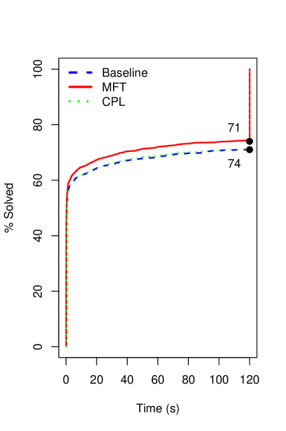
Figure 19: Comparing percent of instances solved with different heuristic profiles.

9 Conclusions

Previous attempts at optimal task scheduling through branch-and-bound methods have used a state-space model which we refer to as exhaustive list scheduling. This state-space model is limited by its high potential for producing duplicate states. In this paper, we have proposed a new state-space model which approaches the problem of task scheduling with communication delays in two distinct phases: allocation, and ordering. In the allocation phase, we assign each task to a processor by searching through all possible groupings of tasks. In the ordering phase, with an allocation already decided, we assign a start time to each task by investigating each possible ordering of the tasks on their processors. Using a priority ordering on processors, and thereby fixing the sequence in which independent tasks must be scheduled, we are able to avoid the production of any duplicate states.

Our evaluation suggests that the AO model allows for superior performance in the majority of problem instances, as searches using the new model were significantly more likely to reach a successful conclusion within a two minute time limit. Along with pruning techniques and optimisations previously used with ELS, a new graph reversal optimisation leads to much higher success rates with Join and In-Tree graph structures. Finally, the more complex Minimum Finish Time heuristic for the allocation phase of AO was found to produce a significant advantage over a simpler heuristic. In this work, the majority of pruning techniques for ELS have either been adapted to AO, or made obsolete by its lack of duplicates. However, entirely new pruning techniques which are only possible under the AO model are likely to be able to be found. Application of these new techniques may allow AO to further improve.

The AO state-space model’s lack of duplicates means that branch-and-bound algorithms searching it do not require the use of additional data structures for duplicate detection. This suggests that AO may have an advantage over ELS when using a low-memory algorithm such as depth-first branch-and-bound. Parallel branch-and-bound is also likely to benefit from the AO model, as the lack of duplicate detection means a decreased need for synchronisation.

References

- [1] B. Veltman, B. J. Lageweg, J. K. Lenstra, Multiprocessor Scheduling with Communication Delays 16 (2-3) (1990) 173–182.
- [2] V. Sarkar, Partitioning and scheduling parallel programs for multiprocessors, MIT press, 1989.
- [3] T. Hagras, J. Janecek, A high performance, low complexity algorithm for compile-time task scheduling in heterogeneous systems, Parallel Computing 31 (7) (2005) 653–670.
-
[4]
T. Yang, A. Gerasoulis,
List
scheduling with and without communication delays, Parallel Computing
19 (12) (1993) 1321–1344.
URL http://www.sciencedirect.com/science/article/pii/016781919390079Z - [5] J.-J. Hwang, Y.-C. Chow, F. D. Anger, C.-Y. Lee, Scheduling Precedence Graphs in Systems with Interprocessor Communication Times, SIAM J. Comput. 18 (2) (1989) 244–257.
- [6] O. Sinnen, Task Scheduling for Parallel Systems (Wiley Series on Parallel and Distributed Computing), Wiley-Interscience, 2007.
- [7] M. Drozdowski, Scheduling for Parallel Processing, 1st Edition, Springer Publishing Company, Incorporated, 2009.
- [8] A. Z. Semar Shahul, O. Sinnen, Scheduling task graphs optimally with A*, Journal of Supercomputing 51 (3) (2010) 310–332.
- [9] M. Orr, O. Sinnen, A duplicate-free state-space model for optimal task scheduling, in: Proc. of 21st Int. European Conference on Parallel and Distributed Computing (Euro-Par 2015), Vol. 9233 of Lecture Notes in Computer Science, Springer, Vienna, Austria, 2015.
- [10] A. Bundy, L. Wallen, Branch-and-bound algorithms, in: A. Bundy, L. Wallen (Eds.), Catalogue of Artificial Intelligence Tools, Symbolic Computation, Springer Berlin Heidelberg, 1984, pp. 12–12.
- [11] N. J. N. P. E. Hart, B. Raphael, A formal basis for the heuristic determination of minimum cost paths, IEEE Transactions on Systems, Science, and Cybernetics SSC-4 (2) (1968) 100–107.
-
[12]
O. Sinnen,
Reducing
the solution space of optimal task scheduling, Computers & Operations
Research 43 (0) (2014) 201 – 214.
doi:http://dx.doi.org/10.1016/j.cor.2013.09.004.
URL http://www.sciencedirect.com/science/article/pii/S0305054813002542 - [13] E. Chan, The foundations of thread-level parallelism in the supermatrix runtime system.
- [14] J. Kurzak, H. Ltaief, J. Dongarra, R. M. Badia, Scheduling dense linear algebra operations on multicore processors, Concurrency and Computation: Practice and Experience 22 (1) (2010) 15–44.
- [15] M.-Y. Wu, D. D. Gajski, Hypertool: A programming aid for message-passing systems, IEEE transactions on parallel and distributed systems 1 (3) (1990) 330–343.
-
[16]
Y.-K. Kwok, I. Ahmad,
Benchmarking the task
graph scheduling algorithms, in: Proc. of Int. Par. Processing
Symposium/Symposium on Par. and Distributed Processing (IPPS/SPDP-98),
Orlando, Florida, USA, 1998, pp. 531–537.
URL http://www.eee.hku.hk/ ykwok/publications.html - [17] Y.-K. Kwok, I. Ahmad, Dynamic critical-path scheduling: An effective technique for allocating task graphs to multiprocessors, IEEE transactions on parallel and distributed systems 7 (5) (1996) 506–521.
- [18] A. Gerasoulis, T. Yang, A comparison of clustering heuristics for scheduling directed acyclic graphs on multiprocessors, Journal of Parallel and Distributed Computing 16 (4) (1992) 276–291.
- [19] Y.-K. Kwok, I. Ahmad, On multiprocessor task scheduling using efficient state space search approaches, Journal of Parallel and Distributed Computing 65 (12) (2005) 1515–1532.
- [20] A. A. El Cadi, R. B. Atitallah, S. d. Hanafi, N. Mladenović, A. Artiba, New mip model for multiprocessor scheduling problem with communication delays, Optimization Letters (2014) 1–17.
- [21] S. Mallach, Improved mixed-integer programming models for multiprocessor scheduling with communication delays.
- [22] S. Venugopalan, O. Sinnen, Integer linear programming for the multiprocessor scheduling problem with communication delays, IEEE Transactions on Parallel and Distributed Systems 16 (1) (2015) 142–151. doi:10.1109/TPDS.2014.2308175.
- [23] S. Lin, Computer solutions of the traveling salesman problem, The Bell System Technical Journal 44 (10) (1965) 2245–2269.
- [24] J. Munkres, Algorithms for the assignment and transportation problems, Journal of the society for industrial and applied mathematics 5 (1) (1957) 32–38.
- [25] B. Borchers, J. Furman, A two-phase exact algorithm for max-sat and weighted max-sat problems, Journal of Combinatorial Optimization 2 (4) (1998) 299–306.
- [26] P. M. Pardalos, T. Mavridou, J. Xue, The graph coloring problem: A bibliographic survey, in: Handbook of combinatorial optimization, Springer, 1998, pp. 1077–1141.
- [27] R. A. Walas, R. G. Askin, An algorithm for nc turret punch press tool location and hit sequencing, IIE Transactions 16 (3) (1984) 280–287.
- [28] M. J. Brusco, S. Stahl, Branch-and-bound applications in combinatorial data analysis, Springer Science & Business Media, 2006.
-
[29]
C. Ronse, Closures on
partial partitions from closures on sets, Mathematica Slovaca 63 (5) (2013)
959–978.
doi:10.2478/s12175-013-0147-9.
URL http://dx.doi.org/10.2478/s12175-013-0147-9 - [30] M. STEPHEN, On some numbers related to the bell numbers, Canadian Mathematical Bulletin 17 (5) (1975) 733.
- [31] D. Berend, T. Tassa, Improved bounds on bell numbers and on moments of sums of random variables, Probability and Mathematical Statistics 30 (2) (2010) 185–205.
- [32] T. Ibaraki, On the computational efficiency of branch-and-bound algorithms, Journal of the Operations Research Society of Japan 20 (1) (1977) 16–35.
- [33] R. Crainic, Lecun, Parallel branch-and-bound algorithms, in: E.-G. Talbi (Ed.), Parallel combinatorial optimization, Vol. 58, John Wiley & Sons, 2006.
-
[34]
O. Sinnen, Reducing the
solution space of optimal task scheduling, Comput. Oper. Res. 43 (2014)
201–214.
doi:10.1016/j.cor.2013.09.004.
URL http://dx.doi.org/10.1016/j.cor.2013.09.004