Construction and Decoding of Product
Codes with Non-Systematic Polar Codes

Abstract

Product codes are widespread in optical communications, thanks to their high throughput and good error-correction performance. Systematic polar codes have been recently considered as component codes for product codes. In this paper, we present a novel construction for product polar codes based on non-systematic polar codes. We prove that the resulting product code is actually a polar code, having a frozen set that is dependent on the frozen sets of the component polar codes. We propose a low-complexity decoding algorithm exploiting the dual nature of the constructed code. Performance analysis and simulations show high decoding speed, that allows to construct long codes while maintaining low decoding latency. The resulting high throughput and good error-correction performance are appealing for optical communication systems and other systems where high throughput and low latency are required.

I Introduction

Polar codes [1] are capacity-achieving linear block codes based on the polarization phenomenon, that makes bit channels either completely noisy or completely noiseless as code length tends to infinity. While optimal at infinite code length, the error-correction performance of polar codes under successive cancellation (SC) decoding degrades at practical code lengths. Moreover, SC-based decoding algorithms are inherently sequential, which results in high dependency of decoding latency on code length. List decoding was proposed in [2] to improve SC performance for practical code lengths: the resulting SC-List (SCL) algorithm exhibits enhanced error-correction performance, at the cost of higher decoder latency and complexity.

Product codes [3] are parallel concatenated codes often used in optical communication systems for their good error-correction performance and high throughput, thanks to their highly parallelizable decoding process. To exploit this feature, systematic polar codes have been concatenated with short block codes as well as LDPC codes [4, 5]. This concatenation allows the construction of very long product codes based on the polarization effect: to fully exploit the decoding parallelism, a high number of parallel decoders for the component codes need to be instantiated, leading to a high hardware cost. Authors in [6] propose to use two systematic polar codes in the concatenation scheme in order to simplify the decoder structure. Soft cancellation (SCAN) [7] and belief propagation (BP) [5] can be used as soft-input / soft-output decoders for systematic polar codes, at the cost of increased decoding complexity compared to SC. Recently, SCL decoding has been proposed as a valid alternative to SCAN and BP [8], while authors in [9] propose to use irregular systematic polar codes to further increase the decoding throughput.

In this paper, we show that the nature of polar codes inherently induces the construction of product codes that are not systematic. In particular, we show that the product of two polar codes is a polar code, that can be designed and decoded as a product code. We propose a code construction approach and a low-complexity decoding algorithm that makes use of the observed dual interpretation of polar codes. Both analysis and simulations show that the proposed code construction and decoding approaches allow to combine high decoding speed and long codes, resulting in high-throughput and good error-correction performance suitable for optical communications.

II Preliminaries

II-A Polar Codes

Polar codes are linear block codes based on the polarization effect of the kernel matrix $T_{2}=\left[\begin{smallmatrix}1&0\\ 1&1\end{smallmatrix}\right]$. A polar code of length $N=2^{n}$ and dimension $K$ is defined by the transformation matrix $T_{N}=T_{2}^{\otimes n}$, given by the $n$-fold Kronecker power of the polarization kernel, and a frozen set $\mathcal{F}\subset\{1,\dots,N\}$ composed of $N-K$ elements. Codeword $x=[x_{0},x_{1},\ldots,x_{N-1}]$ is calculated as

$$x=u\cdot T_{N}\text{,}$$ (1)

where the input vector $u=[u_{0},u_{1},\ldots,u_{N-1}]$ has the $N-K$ bits in the positions listed in $\mathcal{F}$ set to zero, while the remaining $K$ bits carry the information to be transmitted. The frozen set is usually designed to minimize the error probability under SC decoding, such that information bits are stored in the most reliable bits, defining the information set $\mathcal{I}=\mathcal{F}^{C}$. Reliabilities can be calculated in various ways, e.g. via Monte Carlo simulation, by tracking the Batthacharyya parameter, or by density evolution under a Gaussian approximation [10]. The generator matrix $G$ of a polar code is calculated from the transformation matrix $T_{N}$ by deleting the rows of the indices listed in the frozen set.

SC decoding [1] can be interpreted as a depth-first binary tree search with priority given to the left branches. Each node of the tree receives from its parent a soft information vector, that gets processed and transmitted to the left and right child nodes. Bits are estimated at leaf nodes, and hard estimates are propagated from child to parent nodes. While optimal for infinite codes, SC decoding exhibits mediocre performance for short codes. SCL decoding [2] maintains $L$ parallel codeword candidates, improving decoding performance of polar codes for moderate code lengths. The error-correction performance of SCL can be further improved by concatenating the polar code with a cyclic redundancy check (CRC), that helps in the selection of the final candidate.

II-B Product Codes

Product codes were introduced in [3] as a simple and efficient way to build very long codes on the basis of two or more short block component codes. Even if it is not necessary, component codes are usually systematic in order to simplify the encoding. In general, given two systematic linear block codes $\mathcal{C}_{r}$ and $\mathcal{C}_{c}$ with parameters $(N_{r},K_{r})$ and $(N_{c},K_{c})$ respectively, the product code $\mathcal{P}=\mathcal{C}_{c}\times\mathcal{C}_{r}$ of length $N=N_{r}N_{c}$ and dimension $K=K_{r}K_{c}$ is obtained as follows. The $K$ information bits are arranged in a $K_{c}\times K_{r}$ matrix $U$, then code $\mathcal{C}_{r}$ is used to encode the $K_{c}$ rows independently. Afterwards, the $N_{r}$ columns obtained in the previous step are encoded independently using code $\mathcal{C}_{c}$. The result is a $N_{c}\times N_{r}$ codeword matrix $X$, where rows are codewords of code $\mathcal{C}_{r}$ and columns are codewords of code $\mathcal{C}_{c}$, calculated as

$$X=G_{c}^{T}\cdot U\cdot G_{r},$$ (2)

where $G_{r}$ and $G_{c}$ are the generator matrices of codes $\mathcal{C}_{r}$ and $\mathcal{C}_{c}$ respectively. Alternatively, the generator matrix of $\mathcal{P}$ can be obtained taking the Kronecker product of the generator matrices of the two component codes as $G=G_{c}\otimes G_{r}$ [11].

Product codes can be decoded by sequentially decoding rows and column component codes, and exchanging information between the two phases. Soft-input/soft-output algorithms are used to improve the decoding performance by iterating the decoding of rows and columns and exchanging soft information between the two decoders [12]. Since no information is directly exchanged among rows (columns), the decoding of all row (column) component codes can be performed concurrently.

III Product Polar Codes Design

Figure 1: Input matrix $U$ for a product polar code.

Product codes based on polar codes have been proposed in literature, using systematic polar codes as one of the two component codes or as both. However, the peculiar structure of polar codes has never been exploited in the construction of the product code. Both polar and product codes are defined through the Kronecker product of short and simple blocks, that are used to construct longer and more powerful codes. In the following, we prove that the product of two non-systematic polar codes is still a polar code, having a peculiar frozen set obtained on the basis of the component polar codes. This design can be extended to multi-dimensional product codes.

Let us define two polar codes $\mathcal{C}_{r}$ and $\mathcal{C}_{c}$ of parameters $(N_{r},K_{r})$ and $(N_{c},K_{c})$ with transformation matrices $T_{N_{r}}$ and $T_{N_{c}}$ respectively, where $N_{c}=2^{n_{c}}$ and $N_{r}=2^{n_{r}}$, and $\mathcal{F}_{r}$ and $\mathcal{F}_{c}$ are the respective frozen sets. The product polar code $\mathcal{P}=\mathcal{C}_{c}\times\mathcal{C}_{r}$ is generated as follows. An $N_{c}\times N_{r}$ input matrix $U$ is generated having zeros in the columns listed in $\mathcal{F}_{r}$ and in the rows listed in $\mathcal{F}_{c}$ as depicted in Figure 1. Input bits are stored in the remaining $K_{r}K_{c}$ entries of $U$, row first, starting from the top left entry. Encoding is performed as for product codes: the rows of $U$ are encoded independently using polar code $\mathcal{C}_{r}$, namely through matrix multiplication by the transformation matrix $T_{N_{r}}$, obtaining matrix $U_{r}$. Then, the columns of $U_{r}$ are encoded independently using $\mathcal{C}_{c}$. The encoding order can be inverted performing column encoding first and row encoding next without changing the results. The resulting codeword matrix $X$ can be expressed as

$$X=T_{N_{c}}^{T}\cdot U\cdot T_{N_{r}}.$$ (3)

In order to show that this procedure creates a polar code, let us vectorize the input and codeword matrices $U$ and $X$, converting them into row vectors $u$ and $x$. This operation is performed by the linear transformation $\operatorname*{row}(\cdot)$, which converts a matrix into a row vector by juxtaposing its rows head-to-tail. This transformation is similar to the classical vectorization function $\operatorname*{vec}(\cdot)$ converting a matrix into a column vector by juxtaposing its columns head-to-tail. However, before proving our claim, we need to extend a classical result of $\operatorname*{vec}(\cdot)$ function to $\operatorname*{row}$ function.

Lemma 1.

Given three matrices $A$, $B$, $C$ such that $A\cdot B\cdot C$ is defined, then

$$\operatorname*{row}(A\cdot B\cdot C)=\operatorname*{row}(B)\cdot(A^{T}\otimes C).$$ (4)

Proof.

The compatibility of vectorization with the Kronecker product is well known, and is used to express matrix multiplication $A\cdot B\cdot C$ as a linear transformation $\operatorname*{vec}(A\cdot B\cdot C)=(C^{T}\otimes A)\cdot\operatorname*{vec}(B)$. Moreover, by construction we have that $\operatorname*{vec}(A^{T})=(\operatorname*{row}(A))^{T}$. As a consequence,

$$\operatorname*{row}(A\cdot B\cdot C) =(\operatorname*{vec}((A\cdot B\cdot C)^{T}))^{T}$$

$$=(\operatorname*{vec}(C^{T}\cdot B^{T}\cdot A^{T}))^{T}$$

$$=((A\otimes C^{T})\cdot\operatorname*{vec}(B^{T}))^{T}$$

$$=(\operatorname*{vec}(B^{T}))^{T}\cdot(A\otimes C^{T})^{T}$$

$$=\operatorname*{row}(B)\cdot(A^{T}\otimes C).$$

∎

Equipped with Lemma 1 we can now prove the following proposition:

Proposition 1.

The $(N,K)$ product code $\mathcal{P}$ defined by the product of two non-systematic polar codes as $\mathcal{P}=\mathcal{C}_{c}\times\mathcal{C}_{r}$ is a non-systematic polar code having transformation matrix $T_{N}=T_{N_{c}}\otimes T_{N_{r}}$ and frozen set

$$\mathcal{F}=\arg\min(i_{c}\otimes i_{r}),$$ (5)

where $i_{r}$ ($i_{c}$) is a vector of length $N_{r}$ ($N_{c}$) having zeros in the positions listed in $\mathcal{F}_{r}$ ($\mathcal{F}_{c}$) and ones elsewhere.

Proof.

To prove the proposition we have to show that $x=\operatorname*{row}(X)$ is the codeword of a polar code, providing its frozen set and transformation matrix. If $u=\operatorname*{row}(U)$, Lemma 1 shows that

$$x =\operatorname*{row}(X)$$

$$=\operatorname*{row}(T_{N_{c}}^{T}\cdot U\cdot T_{N_{r}})$$

$$=\operatorname*{row}(U)\cdot(T_{N_{c}}\otimes T_{N_{r}})$$

$$=u\cdot T_{N}.$$

By construction, input vector $u$ has zero entries in positions imposed by the structure of the input matrix $U$, and (5) follows from the definition of $U$; with a little abuse of notation, we use the $\arg\min$ function to return the set of the indices of vector $i=i_{c}\otimes i_{r}$ for which the entry is zero. Finally, $T_{N}=T_{N_{c}}\otimes T_{N_{r}}=T_{2}^{\otimes(n_{c}+n_{r})}$ is the transformation matrix of a polar code of length $N=2^{n_{c}+n_{r}}$. ∎

Proposition 1 shows how to design a product polar code on the basis of the two component polar codes. The resulting product polar code $\mathcal{P}$ has parameters $(N,K)$, with $N=N_{r}N_{c}$ and $K=K_{r}K_{c}$, and frozen set $\mathcal{F}$ designed according to (5). The encoding of $\mathcal{P}$ can be performed in $O(\log N)$ steps exploiting the structure of $T_{N}$. The sub-vectors $x_{r}^{i}$ and $x_{c}^{j}$ corresponding to the $i$-th row and the $j$-th column of $X$ represent codewords of polar codes $\mathcal{C}_{r}$ and $\mathcal{C}_{c}$ respectively. It is worth noticing that the frozen set identified for the product polar code is suboptimal, w.r.t. SC decoding, compared to the one calculated for a polar code of length $N$. On the other hand, this frozen set allows to construct a polar code as a result of the product of two shorter polar codes, that can be exploited at decoding time to reduce the decoding latency, as shown in Section IV-B. We also conjecture the possibility to invert the product polar code construction, decomposing a polar code as the product of two or more shorter polar codes.

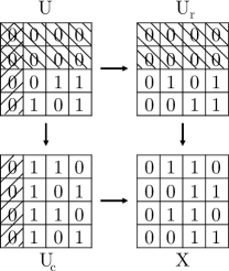
Figure 2: Example of product polar code design and encoding.

Figure 2 shows the encoding of a product polar code generated by a $(4,2)$ polar code with frozen set $\mathcal{F}_{c}=\{0,1\}$ as column code $\mathcal{C}_{c}$ and a $(4,3)$ polar code with frozen set $\mathcal{F}_{r}=\{0\}$ as row code $\mathcal{C}_{r}$. This defines a product polar code $\mathcal{P}$ with $N=16$ and $K=6$. According to Proposition 1, its frozen set can be calculated through the Kronecker product of the auxiliary vectors $i_{c}=[0,0,1,1]$ and $i_{r}=[0,1,1,1]$, obtaining $\mathcal{F}=\{0,1,2,3,4,5,6,7,8,12\}$. We recall that the optimal frozen set for a $(16,6)$ polar code is given by $\mathcal{F}^{\prime}=\{0,1,2,3,4,5,6,8,9,10\}$.

IV Low-latency Decoding of Product Polar Codes

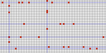
Figure 3: Example of overlapping of $X_{r}$ and $X_{c}$. Red squares represent mismatches, blue lines represent wrong estimations identified by Algorithm 1.

In this Section, we present a two-step, low-complexity decoding scheme for the proposed polar product codes construction, based on the dual nature of these codes. We propose to initially decode the code as a product code (step 1), and in case of failure to perform SC decoding on the full polar code (step 2). The product code decoding algorithm of step 1 exploits the soft-input / hard-output nature of SC decoding to obtain a low complexity decoder for long codes. We then analyze the complexity and expected latency of the presented decoding approach.

IV-A Two-Step Decoding

The first decoding step considers the polar code as a product code. Vector $y$ containing the log-likelihood ratios (LLRs) of the $N$ received bits is rearranged in the $N_{c}\times N_{r}$ matrix $Y$. Every row is considered as a noisy $\mathcal{C}_{r}$ polar codeword, and decoded independently through SC to estimate vector $\hat{u}_{r}$. Each $\hat{u}_{r}$ is re-encoded, obtaining $\hat{x}_{r}=\hat{u}_{r}\cdot T_{N_{r}}$: the $N_{r}$-bit vectors $\hat{x}_{r}$ are then stored as rows of matrix $X_{r}$. The same procedure is applied to the columns of $Y$, obtaining vectors $\hat{x}_{c}=\hat{u}_{c}\cdot T_{N_{c}}$, that are in turn stored as columns of matrix $X_{c}$. In case $X_{r}=X_{c}$, decoding is considered successful; the estimated input vector $\hat{u}$ of code $\mathcal{P}$ can thus be derived inverting the encoding operation, i.e. by encoding vector $\hat{x}=\operatorname*{row}(X_{r})$, since $T_{N}$ is involutory. In case $X_{r}\neq X_{c}$, it is possible to identify incorrect estimations by overlapping $X_{r}$ and $X_{c}$ and observing the pattern of mismatches. Mismatches are usually grouped in strings, as shown in Figure 3, where mismatches are represented by red squares.

Algorithm 1 FindErroneousEstimations

1:  Initialize $\text{ErrRows}=\text{ErrCols}=\emptyset$

2:  $X_{d}=X_{r}\oplus X_{c}$

3:  $\text{NumErrRows}=\text{SumRows}(X_{d})$

4:  $\text{NumErrCols}=\text{SumCols}(X_{d})$

5:  while $\text{NumErrRows}+\text{NumErrCols}>0$ do

6:     $e_{r}=\text{arg max(NumErrRows)}$

7:     $e_{c}=\text{arg max(NumErrCols)}$

8:     if $\text{max(NumErrRows)}>\text{max(NumErrCols)}$ then

9:        $\text{ErrRows}=\text{ErrRows}\cup\{e_{r}\}$

10:        $X_{d}(e_{r},:)=0$

11:     else

12:        $\text{ErrCols}=\text{ErrCols}\cup\{e_{c}\}$

13:        $X_{d}(:,e_{c})=0$

14:     end if

15:     $\text{NumErrRows}=\text{SumRows}(X_{d})$

16:     $\text{NumErrCols}=\text{SumCols}(X_{d})$

17:  end while

18:  return  ErrRows, ErrCols

Even if mismatch patterns are simple to analyze by visual inspection, it may be complex for an algorithm to recognize an erroneous row or column. We propose the greedy Algorithm 1 to accomplish this task. The number of mismatches in each row and column is counted, flagging as incorrect that with the highest count. Next, its contribution is subtracted from the mismatch count of connected rows or columns, and another incorrect one is identified. The process is repeated until all mismatches belong to incorrect rows or columns, the list of which is stored in ErrRows and ErrCols. An example of this identification process is represented by the blue lines in Figure 3.

Incorrect rows can be rectified using correct columns and vice-versa, but intersections of wrong rows and columns cannot. In order to correct these errors, we propose to treat the intersection points as erasures. As an example, in a row, crossing points with incorrect columns have their LLR set to 0, while intersections with correct columns set the LLR to $+\infty$ if the corresponding bit in $X_{c}$ has been decoded as $0$, and to $-\infty$ if the bit is $1$. The rows and columns flagged as incorrect are then re-decoded, obtaining updated $X_{r}$ and $X_{c}$. This procedure is iterated a number $t$ of times, or until $X_{r}=X_{c}$.

In case $X_{r}\neq X_{c}$ after $t$ iterations, the first step returns a failure. In this case, the second step of the algorithm is performed, namely the received vector $y$ is decoded directly, considering the complete length-$N$polar code $\mathcal{P}$.

The proposed two-step decoding approach is summarized in Algorithm 2. Any polar code decoder can be used at lines 3,4 and 16. However, since a soft output is not necessary, and the decoding process can be parallelized, simple, sequential and non-iterative SC-based algorithms can be used instead of the more complex BP and SCAN.

Algorithm 2 TwoStepDecoding

1:  Initialize $Y_{r}=Y_{c}=Y$

2:  for $w=1\dots t$ do

3:     $\hat{X}_{r}=\text{DecodeRows}(Y)$

4:     $\hat{X}_{c}=\text{DecodeCols}(Y)$

5:     if $X_{r}==X_{c}$ then

6:        $\hat{x}=\operatorname*{row}(X_{r})$

7:        return  $\hat{u}=\text{PolarEncoding}(\hat{x})$

8:     else

9:        FindErroneousEstimations

10:     end if

11:     $Y_{r}=(-2\hat{X}_{c}+1)\cdot\infty$

12:     $Y_{c}=(-2\hat{X}_{r}+1)\cdot\infty$

13:     $Y_{r}(:,\text{ErrCols})=0$

14:     $Y_{c}(\text{ErrRows},:)=0$

15:  end for

16:  return  $\hat{u}=\text{Decode}(y)$

IV-B Decoding Latency and Complexity

The proposed two-step decoding of product polar codes allows to split the polar decoding process into $N_{r}+N_{c}$ shorter, independent decoding processes, whose hard decisions are compared and combined together, using the long polar code decoding only in case of failure. Let us define as $\Delta_{N}$ the number of time steps required by an SC-based algorithm to decode a polar code of length $N$. For the purpose of latency analysis, we suppose the decoder to have unlimited computational resources, allowing a fully parallel implementation of decoding algorithms. Using Algorithm 2 to decode component codes, the expected number of steps for the proposed two-step decoder for a code of length $N=N_{c}N_{r}$ is given by

$$\Delta^{\rm P}_{N}=t_{avg}\Delta_{\max(N_{r},N_{c})}+\gamma\Delta_{N}~{},$$ (6)

where $t_{avg}\leq t$ is the average number iterations, and $\max(N_{r},N_{c})$ assumes that the decoding of row and column component codes is performed at the same time. The parameter $\gamma$ is the fraction of decoding attempts in which the second decoding step was performed. It can be seen that as long as $\gamma\approx 0$ and $t_{avg}<<N/\max(N_{r},N_{c})$, then $\Delta^{\rm P}_{N}$ is substantially smaller than $\Delta_{N}$.

The structure of parallel and partially-parallel SC-based decoders is based on a number of processing elements performing LLR and hard decision updates, and on dedicated memory structures to store final and intermediate values. Given the recursive structure of polar codes, decoders for shorter codes are naturally nested within decoders for longer codes. In the same way, the main difference between long and short code decoders is the amount of memory used. Thus, not only a high degree of resource sharing can be expected between the first and second decoding step; the parallelization available during the first decoding step implies that the same hardware can be used in the second step, with minor overhead.

V Performance Results

The dual nature of product polar codes can bring substantial speedup in the decoding; on the other hand, given a time constraint, longer codes can be decoded, leading to improved error-correction performance. In this Section, we present decoding speed and error-correction performance analysis, along with simulation results. We assume an additive white Gaussian noise (AWGN) channel with binary phase-shift keying (BPSK) modulation, while the two component codes have the same parameters, i.e. $N_{r}=N_{c}$ and $K_{r}=K_{c}$.

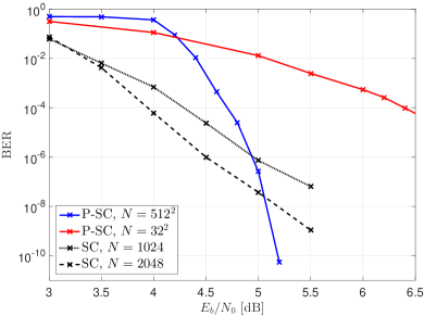
Figure 4: BER comparison for SC and P-SC, for codes of rate $R=(7/8)^{2}$.

V-A Error-Correction Performance

As explained in Section III, the frozen set identified for the code of length $N$ is suboptimal for product decoding of polar codes, that relies on the frozen set seen by component codes. On the other hand, a frozen set that can help product decoding leads to error-correction performance degradation when standard polar code decoding is applied.

Figure 4 portrays the bit error rate (BER) for different codes under P-SC decoding, i.e. the proposed two-step decoding with SC as the component decoder, with parameter $t=4$, while $N=512^{2}=262144$ and $N=32^{2}=1024$ with rate $R=(7/8)^{2}$. As a reference, Figure 4 displays also curves obtained with SC decoding of a polar code of length $N=1024$ and $N=2048$, with the same rate $R=(7/8)^{2}$, designed according to [1]. As expected due to the suboptimality of the frozen set, P-SC degrades the error correction performance with respect to standard SC decoding when compared to codes with the same code length $N$. However, the speedup achieved by P-SC over standard SC allows to decode longer codes within the same time constraint: consequently, we compare codes with similar decoding latency. SC decoding of $N=2048$ and $N=1024$ codes has a decoding latency similar to that of a conservative estimate for P-SC decoding of the $N=512^{2}$ code. The steeper slope imposed by the longer code can thus be exploited within the same time frame as the shorter codes: the BER curves are shown to cross at around $\text{BER}\simeq 10^{-7}$.

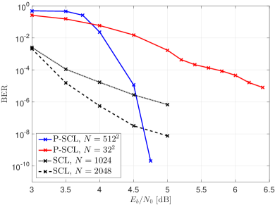
Figure 5: BER comparison for SCL and P-SCL, for codes of rate $R=(7/8)^{2}$ and $L=8$.

Figure 5 depicts the BER curves for the same codes, obtained through SCL and P-SCL decoding with a list size $L=8$, and no CRC. The more powerful SCL algorithm leads to an earlier waterfall region for all codes, with a slope slightly gentler than that of SC. The P-SCL curve crosses the SCL ones around similar BER points as in Figure 4, but at lower $E_{b}/N_{0}$.

V-B Decoding Latency

To begin with, we study the evolution of the parameters $\gamma$ and $t_{avg}$ in (6) under SC decoding. Figure 6 depicts the value of $\gamma$ measured at different $E_{b}/N_{0}$, for various code lengths and rates. The codes have been decoded with the proposed two-step decoding approach, considering $t=4$ maximum iterations. As $E_{b}/N_{0}$ increases, the number of times SC is activated rapidly decreases towards $0$, with $\gamma<10^{-3}$ at a BER orders of magnitude higher than the working point for optical communications, which is the target scenario for the proposed construction. Simulations have shown that the slope with which $\gamma$ tends to $0$ changes depending on the value of $t$; as $t$ increases, so does the steepness of the $\gamma$ curve. Regardless of $t$, $\gamma$ tends to $0$ as the channel conditions improve.

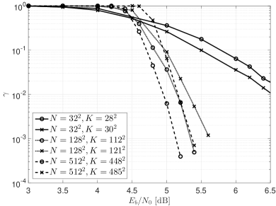
Figure 6: Evolution of $\gamma$ with codes of different length and rate, SC component decoding, $t=4$, $N_{r}=N_{c}$, $R_{r}=R_{c}$.

The first decoding step is stopped as soon as $X_{r}=X_{c}$, or if the maximum number of iterations $t$ has been reached. Through simulation, we have observed that the average number of iterations $t_{avg}$ follows a behavior similar to that of $\gamma$, and tends to $1$ as $E_{b}/N_{0}$ increases. It is worth noting that similar considerations apply when a decoding algorithm different than SC is used, as long as the same decoder is applied to the component codes and the length-$N$ code. The trends observed with SC for $\gamma$ and $t_{avg}$ are found with P-SCL as well, and we can safely assume that similar observations can be made with other SC-based decoding algorithms.

Table I reports $\Delta_{N}$ required by standard SC and SCL decoders, as well as for the proposed two-step decoder P-SC and P-SCL, at different code lengths and rates. Assuming no restrictions of available resources, the number of time steps required by SC decoding is $\Delta^{\rm SC}_{N}=2N-2$, that becomes $\Delta^{\rm SCL}_{N}=2N+K-2$ for SCL decoding [13]. For P-SC and P-SCL, $\Delta^{\rm P}_{N}$ is evaluated for worst case (WC), that assumes $t_{avg}=t$ and $\gamma=1$, and best case (BC), that assumes $t_{avg}=1$ and $\gamma=0$. Simulation results show that $\Delta^{\rm P}_{N}$ tends to the asymptotic limit represented by BC decoding latency as the BER goes towards optical communication working point. As an example, for $N=512^{2}=262144$, $K=448^{2}=200704$ with P-SC, at $\text{BER}\simeq 2.5\cdot 10^{-7}$, i.e. approximately eight orders of magnitude higher than the common target for optical communications, $\gamma\approx 6\cdot 10^{-3}$ and $t_{avg}=1.1$, leading to $\Delta_{N}^{\rm P-SC}=5967$. This value is equivalent to $1.1\%$ of standard decoding time $\Delta_{N}^{\rm SC}$, while the BC latency is $0.2\%$ of $\Delta_{N}^{\rm SC}$. At $\text{BER}\simeq 10^{-15}$, it is safe to assume that the actual decoding latency is almost equal to BC.

TABLE I: Time step analysis for standard and two-step decoding.

Code	$\Delta^{\rm SC}_{N}$	$\Delta^{\rm P-SC}_{N}$		$\Delta^{\rm SCL}_{N}$	$\Delta^{\rm P-SCL}_{N}$
$N$,$K$		WC	BC		WC	BC
$1024,784$	2046	2294	62	2830	3190	90
$1024,841$	2046	2294	62	2876	3240	91
$4096,3136$	8190	8694	126	11326	12054	182
$4096,3249$	8190	8694	126	11508	12244	184
$16384,12544$	32766	33782	254	45310	46774	366
$16384,13225$	32766	33782	254	46038	47518	370
$65536,50176$	131070	133110	510	181246	184182	734
$65536,52900$	131070	133110	510	184155	187119	741
$262144,200704$	524286	528374	1022	724990	730870	1470
$262144,211600$	524286	528374	1022	736623	742555	1483

VI Conclusion

In this paper, we have shown that the product of two non-systematic polar codes results in a polar code whose transformation matrix and frozen set are inferred from the component polar codes. We have then proposed a code construction and decoding approach that exploit the dual nature of the resulting product polar code. The resulting code is decoded first as a product code, obtaining substantial latency reduction, while standard polar decoding is used as post-processing in case of failures. Performance analysis and simulations show that thanks to the high throughput of the proposed decoding approach, very long codes can be targeted, granting good error-correction performance suitable for optical communications. Future works rely on the inversion of the proposed product polar code construction, namely rewriting any polar code as the product of smaller polar codes.

References

- [1] E. Arıkan, “Channel polarization: A method for constructing capacity-achieving codes for symmetric binary-input memoryless channels,” IEEE Transactions on Information Theory, vol. 55, no. 7, pp. 3051–3073, July 2009.
- [2] I. Tal and A. Vardy, “List decoding of polar codes,” IEEE Transactions on Information Theory, vol. 61, no. 5, pp. 2213–2226, May 2015.
- [3] P. Elias, “Error-free coding.,” Transactions of the IRE Professional Group on Information Theory, vol. 4, no. 4, pp. 29–37, 1954.
- [4] M. Seidl and J. B. Huber, “Improving successive cancellation decoding of polar codes by usage of inner block codes,” in IEEE International Symposium on Turbo Codes and Iterative Information Processing (ISTC), Brest, France, September 2010.
- [5] J. Guo, M. Qin, A. G. I Fabregas, and P. H. Siegel, “Enhanced belief propagation decoding of polar codes through concatenation,” in IEEE International Symposium on Information Theory (ISIT), 2014, Honolulu, HI, USA, June 2014.
- [6] D. Wu, A. Liu, Y. Zhang, and Q. Zhang, “Parallel concatenated systematic polar codes,” in Electronics Letters, 2015, vol. 52, pp. 43–45.
- [7] U. U. Fayyaz and J. R. Barry, “Low-complexity soft-output decoding of polar codes,” IEEE Journal on Selected Areas in Communications, vol. 32, no. 5, pp. 958–966, 2014.
- [8] Z. Liu, K. Niu, and J. Lin, “Parallel concatenated systematic polar code based on soft successive cancellation list decoding,” in IEEE International Symposium on Wireless Personal Multimedia Communications (WPMC), Yogyakarta, Indonesia, December 2017.
- [9] T. Koike-Akino, C. Cao, Y. Wang, K. Kojima, D. S. Millar, and K. Parsons, “Irregular polar turbo product coding for high-throughput optical interface,” in Optical Fiber Communication Conference and Exhibition (OFC), San Diego, CA, USA, 2018, p. March.
- [10] H. Vangala, E. Viterbo, and Y. Hong, “A comparative study of polar code constructions for the AWGN channel,” in arXiv preprint arXiv:1501.02473, 2015.
- [11] F. J. MacWilliams and N. J. A. Sloane, The theory of error-correcting codes, Elsevier, 1977.
- [12] R. M. Pyndiah, “Near-optimum decoding of product codes: Block turbo codes,” IEEE Transactions on communications, vol. 46, no. 8, pp. 1003–1010, 1998.
- [13] S. A. Hashemi, C. Condo, and W. J. Gross, “Fast and flexible successive-cancellation list decoders for polar codes,” IEEE Transactions on Signal Processing, vol. 65, no. 21, pp. 5756–5769, October 2017.