Calculation of the electromagnetic scattering by non-spherical particles based on the volume integral equation in the spherical wave function basis

Abstract

The paper presents a method for calculation of non-spherical particle T-matrices based on the volume integral equation and the spherical vector wave function basis, and relies on the Generalized Source Method rationale. The developed method appears to be close to the invariant imbedding approach, and the derivations aims at intuitive demonstration of the calculation scheme. In parallel calculation of single columns of T-matrix is considered in detail, and it is shown that this way not only has a promising potential of parallelization but also yields an almost zero power balance for purely dielectric particles.

1 Introduction

An accurate simulation of the light scattering by non-spherical particles is important for a variety of applications ranging from planetary science to nanoscale power transfer. A number of methods for achieving this goal were developed [1]. When looking from the point of view of “arbitrariness” of possible particle shapes and a range of treatable size parameters the Discreet Dipole Approximation (DDA) and the other Volume Integral Equation (VIE) methods appear to be the most handy while retaining a relative formulation simplicity [2, 3]. The methods are based on the volume integral equation solution to the three-dimensional Helmholtz equation, and a three-dimensional equidistant spatial discretization makes it possible to greatly benefit from fast-Fourier transform based numerical algorithms. That said, the named methods conventionally lack of another property being quite important for applications. They yield and output in form of a response vector given an excitation field vector, while a complete T-matrix [4, 5] is often of interest. The reason is in the mismatch in the field representation, which is the point-wise storage of the spatial field components in case of the DDA/VIE, while the T-matrix is conventionally defined in terms of the spherical vector wave field decomposition.

A possible way to couple the pros of the VIE methods with a direct T-matrix output is to consider the volume integral equation in the spherical vector wave function basis together with a spatial discretization into a set of thin spherical shells instead of small cubic volumes. This approach was considered in [6] within the rationale of the invariant imbedding technique, and further applied in [7, 8, 9] for analysis of atmospheric ice particle light scattering features. The equivalence between the invariant imbedding procedure and the integral-matrix approaches was outlined in [10, 11]. The method represents an interesting alternative to the previously well-developed volume integral methods. This work proposes a different view on the mentioned approach. In addition within the same rationale a numerical approach to calculate single columns of the T-matrix is presented in detail, which was only mentioned in [6]. The latter approach not only possess a potential for parallelization, but also is shown to yield results which meet the energy conservation at very high precision.

In order to trace analogies between the methods in spherical and planar geometries the derivations of this paper are based on the rationale of the Generalized Source Method (GSM) [12], which was applied previously to the grating diffraction problems [13]. Besides, this logic is chosen to support a further introduction of the generalized metric sources in the spherical vector wave basis in analogy with [14, 15], to be described in a next paper. The GSM relies on basis solutions which provide a rigorous way to calculate an output of an arbitrary source current. Here a homogeneous space basis solution (can be read as the homogeneous space Green’s function) is used to develop a scattering matrix algorithm being a counterpart of the invariant imbedding method. Then, a basis solution in a homogeneous spherical layer is used to formulate a scattering vector algorithm yielding single columns of T-matrices [16]. The terms scattering matrix and scattering vector are defined and discussed below. Finally, numerical examples are presented demonstrating an accuracy and convergence rates of the algorithms.

2 Generalized source method

The scattering problem being addressed in this work is schematically demonstrated in Fig. 1. Given a homogeneous scattering particle occupying a closed three-dimensional volume $\Omega_{p}$ and an external time-harmonic electromagnetic field with amplitudes ${\bf E}^{ext}\left(\bm{r}\right)$, ${\bf H}^{ext}\left(\bm{r}\right)$ and frequency $\omega$ excited by some sources ${\bf J}^{ext}\left(\bm{r}\right)$ located outside the spherical domain $\Omega_{R}^{out}=\left\{\bm{r}=\left(r,\theta,\varphi\right):\thinspace r\leq R\right\}\ni\Omega_{p}$ containing the particle, here $\left(r,\theta,\varphi\right)$ are spherical coordinates, one aims at calculation of the total electromagnetic field being a solution of the time-harmonic Maxwell’s equations. This scattering problem is characterized by a spatially inhomogeneous dielectric permittivity $\varepsilon\left(\bm{r}\right)$ which equals to some constant $\varepsilon_{p}$ (possibly complex) inside the volume $\Omega_{p}$, and to real constant $\varepsilon_{s}$ in the surrounding non-absorbing medium $\bm{r}\in\mathbb{R}^{3}\backslash\Omega_{p}$. For simplicity, and aiming at optical applications, within this paper the permeability is considered to be equal to the vacuum permeability $\mu_{0}$.

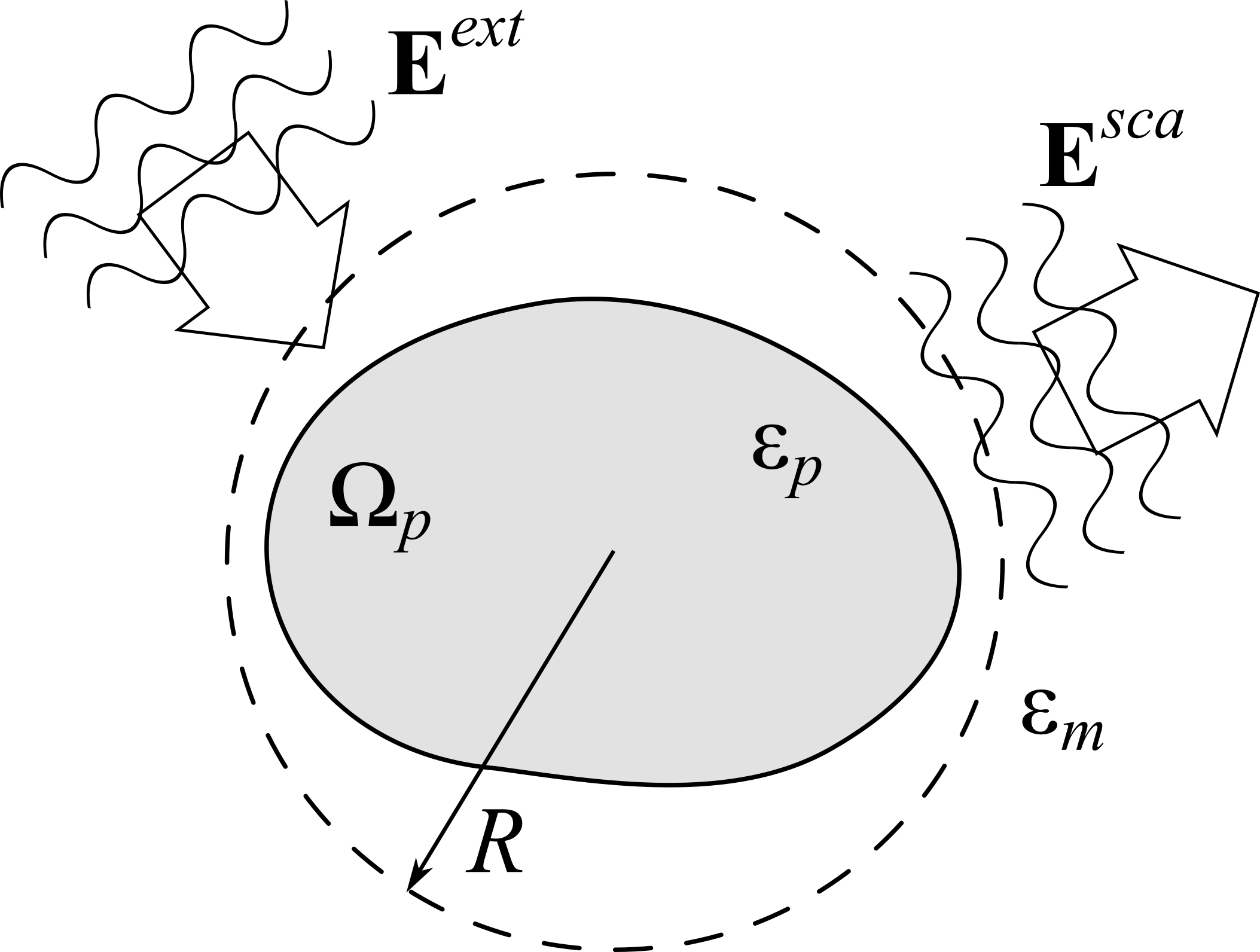
Figure 1: Scattering problem being addressed in this work.

Assume that solution of the electromagnetic scattering problem is known for some basis structure characterized by the function $\varepsilon_{b}\left(\bm{r}\right)$ whatever the sources are, and this solution is given by the linear operator $\mathfrak{S}_{b}$ as follows:

$${\bf E}={\bf E}^{ext}+\mathfrak{S}_{b}\left({\bf J}\left(\bm{r}\right)\right)$$ (1)

Then, in order to find a solution of the initial scattering problem one has to consider a difference between the initial and the basis media which gives rise to the generalized source ${\bf J}_{gen}\left(\bm{r}\right)$, so that the desired self-consistent field ${\bf E}\left(\bm{r}\right)$ appears to meet the following equation

$${\bf E}={\bf E}^{ext}+\mathfrak{S}_{b}\left({\bf J}_{gen}\left(\bm{r}\right)\right)$$ (2)

Conventionally within the volume integral equation methods one takes ${\bf J}_{gen}\left(\bm{r}\right)=-i\omega\left[\varepsilon\left(\bm{r}\right)-\varepsilon_{b}\left(\bm{r}\right)\right]{\bf E}\left(\bm{r}\right)$ [3]. In this work Eq. (2) is enclosed in a similar way.

3 Basis solution

The declared intention to operate with spherical vector wave function decompositions generally restricts the choice of the basis medium to be a set of homogeneous space regions of constant permittivity separated by concentric spherical interfaces. This is due to the fact that the reflection and transmission are described in form of diagonal operators for these basis functions. The basis operator $\mathfrak{S}_{b}$ is explicitly defined by the corresponding Green’s function, (e.g., [17]). Yet, for the methods developed in this work it is sufficient to consider only two cases – a homogeneous isotropic space, and a single spherical layer bounded by two interfaces. This section outlines the basis solution in a homogeneous basis space.

In view of the said assume here $\varepsilon_{b}\left(\bm{r}\right)$ to be constant everywhere. Time-harmonic Maxwell’s equations in the basis medium with extracted factor $\exp\left(-i\omega t\right)$

$$\begin{array}[]{c}\nabla\times{\bf E}\left(\bm{r}\right)-i\omega\mu_{0}{\bf H}\left(\bm{r}\right)=0,\\ \nabla\times{\bf H}\left(\bm{r}\right)+i\omega\varepsilon_{b}{\bf E}\left(\bm{r}\right)={\bf J}\left(\bm{r}\right)\end{array}$$ (3)

yield the Helmholtz equation

$$\nabla\times\nabla\times{\bf E}\left(\bm{r}\right)-k_{b}^{2}{\bf E}\left(\bm{r}\right)=i\omega\mu_{0}{\bf J}\left(\bm{r}\right)$$ (4)

where the wavenumber $k_{b}=\omega\sqrt{\varepsilon_{b}\mu_{0}}$. Given the spherical coordinates $\left(r,\theta,\varphi\right)$ with unit vectors $\hat{\bm{e}}_{r}$, $\hat{\bm{e}}_{\theta}$, and $\hat{\bm{e}}_{\varphi}$, and the modified basis $\left(\hat{\bm{e}}_{r},\hat{\bm{e}}_{+},\hat{\bm{e}}_{-}\right)$ which is related to the spherical one as $\hat{\bm{e}}_{\pm}=\left(\hat{\bm{e}}_{\theta}\pm i\hat{\bm{e}}_{\varphi}\right)/\sqrt{2}$, the eigen solutions of the homogeneous Helmholtz equation are the two sets of spherical vector wave functions (see, e.g., [18]):

$$\mathcal{{\bf\mathcal{M}}}_{nm}^{1,3}\left(k_{b}\bm{r}\right)=i\frac{\sqrt{2n+1}}{2\sqrt{2\pi}}z_{n}^{1,3}\left(k_{b}r\right)\left[\hat{\bm{e}}_{+}d_{m,1}^{n}\left(\theta\right)+\hat{\bm{e}}_{-}d_{m,-1}^{n}\left(\theta\right)\right]\exp\left(im\varphi\right)$$ (5)

$$\mathcal{{\bf\mathcal{N}}}_{nm}^{1,3}\left(k_{b}\bm{r}\right) =\frac{\sqrt{n\left(n+1\right)}}{\sqrt{2\pi}}\frac{z_{n}^{1,3}\left(k_{b}r\right)}{k_{b}r}P_{n}^{m}\left(\theta\right)\exp\left(im\varphi\right)\hat{\bm{e}}_{r}$$

$$+\frac{\sqrt{2n+1}}{2\sqrt{2\pi}}\frac{\tilde{z}{}_{n}^{1,3}\left(k_{b}r\right)}{k_{b}r}\left[\hat{\bm{e}}_{+}d_{m,1}^{n}\left(\theta\right)-\hat{\bm{e}}_{-}d_{m,-1}^{n}\left(\theta\right)\right]\exp\left(im\varphi\right)$$ (6)

Here integer indices $n,m$ are subject to constraints $n\geq 0$, $\left|m\right|\leq n$. $P_{n}^{m}\left(\theta\right)$ are normalized associated Legendre polynomials, $d_{m,\pm 1}^{n}\left(\theta\right)$ are elements of rotation Wigner $d$-matrices [19] with $P_{n}^{m}\left(\theta\right)=\sqrt{\left(2n+1\right)/2}d_{m,0}^{n}\left(\theta\right)$. These functions of the polar angle obey the orthogonality condition, which is read via the Kronecker delta-symbol $\delta_{nm}$:

$$\intop_{0}^{\pi}d_{mq}^{n}\left(\theta\right)d_{mq}^{p}\left(\theta\right)\sin\theta d\theta=\frac{2}{2n+1}\delta_{np}.$$ (7)

Superscripts ”1,3” correspond to regular and radiating wave functions respectively, so that $z_{n}^{1}\equiv j_{n}$ is the regular spherical Bessel function, and $z_{n}^{3}\equiv h_{n}^{(1)}$ is the spherical Henkel function of the first kind. Besides, $\tilde{z}_{n}\left(x\right)=d\left[xz_{n}\left(x\right)\right]/dx$. The rotor operator transforms functions (5), (6) one into another:

$$\begin{array}[]{c}\nabla\times\mathcal{{\bf\mathcal{M}}}_{nm}^{1,3}\left(k_{b}\bm{r}\right)=k_{b}\mathcal{{\bf\mathcal{N}}}_{nm}^{1,3}\left(k_{b}\bm{r}\right)\\ \nabla\times\mathcal{{\bf\mathcal{N}}}_{nm}^{1,3}\left(k_{b}\bm{r}\right)=k_{b}\mathcal{{\bf\mathcal{M}}}_{nm}^{1,3}\left(k_{b}\bm{r}\right)\end{array}$$ (8)

Note that once the center of the spherical coordinate system is fixed, all spherical harmonic decompositions are made relative to this center, and no translations are used in this work.

Solution to the Helmholtz equation (4) in the volume integral form is written via the free-space dyadic Green’s function ${\bf G}\left(\bm{r}-\bm{r}^{\prime}\right)$:

$${\bf E}\left(\bm{r}\right)={\bf E}^{ext}\left(\bm{r}\right)+i\omega\mu_{0}\int{\bf G}\left(\bm{r}-\bm{r}^{\prime}\right){\bf J}\left(\bm{r}^{\prime}\right)d^{3}\bm{r}^{\prime}.$$ (9)

The spherical vector wave expansion of ${\bf G}\left(\bm{r}-\bm{r}^{\prime}\right)$ in terms of (5), (6) is [20]:

$${\bf G}\left(\bm{r}-\bm{r}^{\prime}\right) =-\frac{1}{k_{b}^{2}}\hat{\bm{e}}_{r}^{T}\hat{\bm{e}}_{r}\delta\left(r-r^{\prime}\right)$$

$$+ik_{b}\begin{cases}\sum_{nm}\mathcal{{\bf\mathcal{M}}}_{nm}^{1\ast}\left(k_{b}\bm{r}^{\prime}\right)\mathcal{{\bf\mathcal{M}}}_{nm}^{3}\left(k_{b}\bm{r}\right)+\mathcal{{\bf\mathcal{N}}}_{nm}^{1\ast}\left(k_{b}\bm{r}^{\prime}\right)\mathcal{{\bf\mathcal{N}}}_{nm}^{3}\left(k_{b}\bm{r}\right),&r^{\prime}<r,\\ \sum_{nm}\mathcal{{\bf\mathcal{M}}}_{nm}^{3\ast}\left(k_{b}\bm{r}^{\prime}\right)\mathcal{{\bf\mathcal{M}}}_{nm}^{1}\left(k_{b}\bm{r}\right)+\mathcal{{\bf\mathcal{N}}}_{nm}^{3\ast}\left(k_{b}\bm{r}^{\prime}\right)\mathcal{{\bf\mathcal{N}}}_{nm}^{1}\left(k_{b}\bm{r}\right),&r^{\prime}>r.\end{cases}$$ (10)

where the asterisk $\ast$ stands for complex conjugation. This explicitly defines operator $\mathfrak{S}_{b}$ in Eq. (1). Substitution of the latter expression into the equation (9) shows that the resulting field at any space point is a superposition of the vector spherical waves together with the singular term existent in the source region. With a view of simplifying the following derivation let us introduce the modified field $\tilde{{\bf E}}$, such that $\tilde{E}_{r}=E_{r}-J_{r}/i\omega\mu_{b}$, $\tilde{E}_{\theta,\varphi}\equiv E_{\theta,\varphi}$. Therefore, the solution of the volume integral equation can be written purely as a sum of the regular and outgoing waves

$$\tilde{{\bf E}}\left(\bm{r}\right)={\bf E}^{ext}\left(\bm{r}\right)+\sum_{nm}\left[\tilde{a}_{nm}^{e}\left(r\right){\bf\mathcal{M}}{}_{nm}^{3}\left(k_{b}\bm{r}\right)+\tilde{a}_{nm}^{h}\left(r\right){\bf\mathcal{N}}_{nm}^{3}\left(k_{b}\bm{r}\right)+\tilde{b}_{nm}^{e}\left(r\right){\bf\mathcal{M}}_{nm}^{1}\left(k_{b}\bm{r}\right)+\tilde{b}_{nm}^{h}\left(r\right){\bf\mathcal{N}}_{nm}^{1}\left(k_{b}\bm{r}\right)\right].$$ (11)

Since the sources of the external field ${\bf E}^{ext}\left(\bm{r}\right)$ lie outside the region of interest where the solution field is to be evaluated, this external field is also a superposition of vector spherical waves with constant coefficients being the same as its modified counterpart, i.e., $\tilde{a}_{nm}^{ext,e,h}\equiv a_{nm}^{ext,e,h}$, $\tilde{b}_{nm}^{ext,e,h}\equiv b_{nm}^{ext,e,h}$.

Suppose that the region of interest is a spherical layer $R_{1}\leq r\leq R_{2}$. Then, radially dependent amplitudes in Eq. (11) are written through weighted spherical harmonics of the source components

$$\tilde{a}_{nm}^{e}\left(r\right)=\tilde{a}_{nm}^{ext,e}\left(r\right)+\intop_{k_{b}R_{1}}^{k_{b}r}\left[\mathcal{J}_{+,nm}\left(x\right)+\mathcal{J}_{-,nm}\left(x\right)\right]j_{n}\left(x\right)x^{2}dx$$ (12)

$$\tilde{b}_{nm}^{e}\left(r\right)=\tilde{b}_{nm}^{ext,e}\left(r\right)+\intop_{k_{b}r}^{k_{b}R_{2}}\left[\mathcal{J}_{+,nm}\left(x\right)+\mathcal{J}_{-,nm}\left(x\right)\right]h_{n}^{(1)}\left(x\right)x^{2}dx$$ (13)

$$\tilde{a}_{nm}^{h}\left(r\right)=\tilde{a}_{nm}^{ext,h}\left(r\right)+i\intop_{k_{b}R_{1}}^{k_{b}r}\left\{\left[\mathcal{J}_{+,nm}\left(x\right)-\mathcal{J}_{-,nm}\left(x\right)\right]\tilde{j}_{n}\left(x\right)+\mathcal{J}_{r,nm}\left(x\right)j_{n}\left(x\right)\right\}xdx$$ (14)

$$\tilde{b}_{nm}^{h}\left(r\right)=\tilde{b}_{nm}^{ext,h}\left(r\right)+i\intop_{k_{b}r}^{k_{b}R_{2}}\left\{\left[\mathcal{J}_{+,nm}\left(x\right)-\mathcal{J}_{-,nm}\left(x\right)\right]\tilde{h}_{n}^{(1)}\left(x\right)+\mathcal{J}_{r,nm}\left(x\right)h_{n}^{(1)}\left(x\right)\right\}xdx$$ (15)

where

$$\mathcal{J}_{r,nm}\left(x\right)=\frac{\sqrt{n\left(n+1\right)}}{\sqrt{2\pi}}\intop_{0}^{2\pi}\exp\left(-im\varphi\right)d\varphi\intop_{0}^{\pi}\frac{J_{r}\left(x,\theta,\varphi\right)}{-i\omega\varepsilon_{b}}P_{n}^{m}\left(\theta\right)\sin\theta d\theta$$ (16)

$$\mathcal{J}_{\pm,nm}\left(x\right)=\frac{\sqrt{2n+1}}{2\sqrt{2\pi}}\intop_{0}^{2\pi}\exp\left(-im\varphi\right)d\varphi\intop_{0}^{\pi}\frac{J_{\pm}\left(x,\theta,\varphi\right)}{-i\omega\varepsilon_{b}}d_{m,\pm 1}^{n}\left(\theta\right)\sin\theta d\theta$$ (17)

Here the explicit expressions for the vector spherical wave functions (5,6) were used.

Within this work Eqs. (12)-(15) serve as a starting point for derivation of both methods for the complete T-matrix computation (scattering matrix method) and for T-matrix single column computation (scattering vector method).

4 Equations in the homogeneous basis medium

Following the rationale of the GSM given in Section 2 the basis solution of the previous section should be supplemented with the generalized current related to the field as ${\bf J}_{gen}\left(\bm{r}\right)=-i\omega\left[\varepsilon\left(\bm{r}\right)-\varepsilon_{b}\right]{\bf E}\left(\bm{r}\right)$. Invoking the substitution of the real field with the modified field one can acquire the following matrix relation

$${\bf J}_{gen}\left(\bm{r}\right)=-i\omega\left(\begin{array}[]{ccc}\Delta\varepsilon\left(\bm{r}\right)/\varepsilon\left(\bm{r}\right)&0&0\\ 0&\Delta\varepsilon\left(\bm{r}\right)/\varepsilon_{b}&0\\ 0&0&\Delta\varepsilon\left(\bm{r}\right)/\varepsilon_{b}\end{array}\right)\tilde{{\bf E}}\left(\bm{r}\right)$$ (18)

again providing that the vectors are written in the $\left(\hat{\bm{e}}_{r},\hat{\bm{e}}_{+},\hat{\bm{e}}_{-}\right)$ basis and $\Delta\varepsilon\left(\bm{r}\right)=\varepsilon\left(\bm{r}\right)-\varepsilon_{b}$. Since Eqs. (16), (17) involve spherical harmonics of the source, it will be assumed further that the permittivity functions in Eq. (18) admit the spherical harmonic decomposition

$$\left(\begin{array}[]{c}\Delta\varepsilon\left(\bm{r}\right)/\varepsilon\left(\bm{r}\right)\\ \Delta\varepsilon\left(\bm{r}\right)/\varepsilon_{b}\end{array}\right)=\sum_{nm}\left(\begin{array}[]{c}\left[\Delta\varepsilon\left(\bm{r}\right)/\varepsilon\left(\bm{r}\right)\right]_{nm}\\ \left[\Delta\varepsilon\left(\bm{r}\right)/\varepsilon_{b}\right]_{nm}\end{array}\right)\left(r\right)P_{n}^{m}\left(\theta\right)\exp\left(im\varphi\right)$$ (19)

Substitution of Eqs. (18) and (19) into (16), (17), and subsequently into Eqs. (12)-(15) yields the following self-consistent system of integral equations on the radially dependent amplitudes of the spherical vector wave decomposition of the unknown modified field:

$$\tilde{a}_{nm}^{e}\left(r\right)=\tilde{a}_{nm}^{ext,e}+ i\intop_{k_{b}R_{1}}^{k_{b}r}dx\mathcal{V}_{n1}^{(1)}\left(x\right)\sum_{pq}\left[Q_{nm;pq}^{+}\left(x\right)\left(\tilde{a}_{pq}^{e}\mathcal{V}_{p1}^{(3)}\left(x\right)+\tilde{b}_{pq}^{e}\mathcal{V}_{p1}^{(1)}\left(x\right)\right)\right.$$

$$\left.+Q_{nm;pq}^{-}\left(x\right)\left(\tilde{a}_{pq}^{h}\mathcal{V}_{p2}^{(3)}\left(x\right)+\tilde{b}_{pq}^{h}\mathcal{V}_{p2}^{(1)}\left(x\right)\right)\right],$$ (20)

$$\tilde{b}_{nm}^{e}\left(r\right)=\tilde{b}_{nm}^{ext,e}+ i\intop_{k_{b}r}^{k_{b}R_{2}}dx\mathcal{V}_{n1}^{(3)}\left(x\right)\sum_{pq}\left[Q_{nm;pq}^{+}\left(\tilde{a}_{pq}^{e}\mathcal{V}_{p1}^{(3)}\left(x\right)+\tilde{b}_{pq}^{e}\mathcal{V}_{p1}^{(1)}\left(x\right)\right)\right.$$

$$\left.+Q_{nm;pq}^{-}\left(x\right)\left(\tilde{a}_{pq}^{h}\mathcal{V}_{p2}^{(3)}\left(x\right)+\tilde{b}_{pq}^{h}\mathcal{V}_{p2}^{(1)}\left(x\right)\right)\right],$$ (21)

$$\tilde{a}_{nm}^{h}\left(r\right) =\tilde{a}_{nm}^{ext,h}+i\intop_{k_{b}R_{1}}^{k_{b}r}dx\left\{\mathcal{V}_{n3}^{(1)}\left(x\right)\sum_{pq}Q_{nm;pq}^{r}\left(x\right)\left(\tilde{a}_{pq}^{h}\mathcal{V}_{p3}^{(3)}\left(x\right)+\tilde{b}_{pq}^{h}\mathcal{V}_{p3}^{(1)}\left(x\right)\right)\right.$$

$$\left.-\mathcal{V}_{n2}^{(1)}\left(x\right)\sum_{pq}\left[Q_{nm;pq}^{+}\left(x\right)\left(\tilde{a}_{pq}^{h}\mathcal{V}_{p2}^{(3)}\left(x\right)+\tilde{b}_{pq}^{h}\mathcal{V}_{p2}^{(1)}\left(x\right)\right)+Q_{nm;pq}^{-}\left(x\right)\left(\tilde{a}_{pq}^{e}\mathcal{V}_{p1}^{(3)}\left(x\right)+\tilde{b}_{pq}^{e}\mathcal{V}_{p1}^{(1)}\left(x\right)\right)\right]\right\},$$ (22)

$$\tilde{b}_{nm}^{h}\left(r\right) =\tilde{b}_{nm}^{ext,h}+i\intop_{k_{b}r}^{k_{b}R_{2}}dx\left\{\mathcal{V}_{n3}^{(3)}\left(x\right)\sum_{pq}Q_{nm;pq}^{r}\left(x\right)\left(\tilde{a}_{pq}^{h}\mathcal{V}_{p3}^{(3)}\left(x\right)+\tilde{b}_{pq}^{h}\mathcal{V}_{p3}^{(1)}\left(x\right)\right)\right.$$

$$\left.-\mathcal{V}_{n2}^{(3)}\left(x\right)\sum_{pq}\left[Q_{nm;pq}^{+}\left(x\right)\left(\tilde{a}_{pq}^{h}\mathcal{V}_{p2}^{(3)}\left(x\right)+\tilde{b}_{pq}^{h}\mathcal{V}_{p2}^{(1)}\left(x\right)\right)+Q_{nm;pq}^{-}\left(x\right)\left(\tilde{a}_{pq}^{e}\mathcal{V}_{p1}^{(3)}\left(x\right)+\tilde{b}_{pq}^{e}\mathcal{V}_{p1}^{(1)}\left(x\right)\right)\right]\right\}.$$ (23)

To attain these relations one has to, first, apply the orthogonality of the exponential factors, second, utilize the representation of the integral of three Wigner $d$-functions via the product of two Clebsch-Gordan coefficients $C_{p,q;n,m}^{u,s}$ [19], and, finally, exploit the symmetry relations $C_{p,q;u,s}^{n,m}=\left(-1\right)^{p-q}\sqrt{\left(2n+1\right)/\left(2u+1\right)}C_{p,q;n,-m}^{u,-s}$, and $C_{p,q;n,m}^{u,s}=\left(-1\right)^{n+p-u}C_{p,-q;n,-m}^{u,-s}$. These steps yield the following explicit form of the vectors

$${\bf\mathcal{V}}_{n}^{(1,3)}\left(x\right)=\left(ixz_{n}^{1,3}\left(x\right),\thinspace\tilde{z}_{n}^{1,3}\left(x\right),\thinspace\sqrt{n\left(n+1\right)}z_{n}^{1,3}\left(x\right)\right)^{T},$$ (24)

and the matrix elements

$$Q_{nm;pq}^{r} \left(r\right)=\frac{\left(-1\right)^{q}}{\sqrt{2}}\sqrt{2n+1}\sqrt{2p+1}\sum_{u}\left[\frac{\Delta\varepsilon}{\varepsilon}\right]_{u,m-q}\left(r\right)\frac{C_{p,q;n,-m}^{u,m-q}C_{p,0;n,0}^{u,0}}{\sqrt{2u+1}},$$

$$Q_{nm;pq}^{+} \left(r\right)=\frac{\left(-1\right)^{q}}{\sqrt{2}}\sqrt{2n+1}\sqrt{2p+1}\sum_{n+p-u=even}\left[\frac{\Delta\varepsilon}{\varepsilon_{b}}\right]_{u,m-q}\left(r\right)\frac{C_{p,q;n,-m}^{u,m-q}C_{p,1;n,-1}^{u,0}}{\sqrt{2u+1}},$$ (25)

$$Q_{nm;pq}^{-} \left(r\right)=\frac{\left(-1\right)^{q}}{\sqrt{2}}\sqrt{2n+1}\sqrt{2p+1}\sum_{n+p-u=odd}\left[\frac{\Delta\varepsilon}{\varepsilon_{b}}\right]_{u,m-q}\left(r\right)\frac{C_{p,q;n,-m}^{u,m-q}C_{p,1;n,-1}^{u,0}}{\sqrt{2u+1}}.$$

The summation over the index $u$ in the latter expressions is performed under the constraint $\max\left(\left|n-p\right|,\left|m-q\right|\right)\leq u\leq n+p$ for nonvanishing Clebsch-Gordan coefficients [19].

The equation system (20)-(23) is used further in two ways. First, the next section presents an analysis of the scattering by a thin inhomogeneous spherical shell, which brings the core of the mentioned scattering matrix algorithm being an equivalent of the IIM. Second, this system is solved self-consistently upon discretization over a finite radial interval as a part of the scattering vector algorithm. Note that the integrands in (20)-(23) do not depend on the radial distance $r$ as opposed to the initial volume integral equation (9), and $r$ appears only in the integration limits. This feature will be used below to formulate a linear summation part of the scattering vector algorithm. Also, the external field amplitudes do not depend on $r$, as the basis medium is supposed to be a homogeneous space.

5 Scattering matrix of a thin spherical shell

Let us consider the integration region in Eqs. (20)-(23) be a thin spherical shell of the thickness $\Delta R=R_{2}-R_{1}\ll R_{1},R_{2}$, and having the central point $R_{c}=\left(R_{1}+R_{2}\right)/2$. For the sake of brevity Eqs. (20)-(23) can be rewritten in the following matrix-vector form:

$$\begin{array}[]{c}\bm{\tilde{a}}_{nm}\left(r\right)=\bm{\tilde{a}}_{nm}^{ext}+\intop_{k_{b}R_{1}}^{k_{b}r}dx\sum_{pq}\left[\bm{F}_{nm,pq}^{aa}\left(x\right)\bm{\tilde{a}}_{pq}\left(x\right)+\bm{F}_{nm,pq}^{ab}\left(x\right)\bm{\tilde{b}}_{pq}\left(x\right)\right]\\ \bm{\tilde{b}}_{nm}\left(r\right)=\bm{\tilde{b}}_{nm}^{ext}+\intop_{k_{b}r}^{k_{b}R_{2}}dx\sum_{pq}\left[\bm{F}_{nm,pq}^{ba}\left(x\right)\bm{\tilde{a}}_{pq}\left(x\right)+\bm{F}_{nm,pq}^{bb}\left(x\right)\bm{\tilde{b}}_{pq}\left(x\right)\right]\end{array},\thinspace R_{1}\leq r\leq R_{2}$$ (26)

where $\bm{\tilde{a}}_{nm}=\left(\tilde{a}_{nm}^{e},\thinspace\tilde{a}_{nm}^{h}\right)^{T}$ and $\bm{\tilde{b}}_{nm}=\left(\tilde{b}_{nm}^{e},\thinspace\tilde{b}_{nm}^{h}\right)^{T}$. The matrix operator $\bm{F}$ can be directly written out explicitly on the basis of Eqs. (20)-(23), though it is not required for the purpose of this section. Having reliance on the smallness of $\Delta R$ the integrals can be approximately evaluated at the shell boundaries using the midpoint rule:

$$\begin{array}[]{c}\bm{\tilde{a}}_{nm}\left(k_{b}R_{2}\right)\approx\bm{\tilde{a}}_{nm}^{ext}+ik_{b}\Delta R\sum_{pq}\left[\bm{F}_{nm,pq}^{aa}\left(k_{b}R_{c}\right)\bm{\tilde{a}}_{pq}\left(k_{b}R_{c}\right)+\bm{F}_{nm,pq}^{ab}\left(k_{b}R_{c}\right)\bm{\tilde{b}}_{pq}\left(k_{b}R_{c}\right)\right],\\ \bm{\tilde{b}}_{nm}\left(k_{b}R_{1}\right)\approx\bm{\tilde{b}}_{nm}^{ext}+ik_{b}\Delta R\sum_{pq}\left[\bm{F}_{nm,pq}^{ba}\left(k_{b}R_{c}\right)\bm{\tilde{a}}_{pq}\left(k_{b}R_{c}\right)+\bm{F}_{nm,pq}^{bb}\left(k_{b}R_{c}\right)\bm{\tilde{b}}_{pq}\left(k_{b}R_{c}\right)\right],\end{array}$$ (27)

owing the accuracy of $O\left(\left(\Delta R\right)^{3}\right)$. Amplitude vectors evaluated at the central point $\bm{\tilde{a}}_{pq}\left(k_{b}R_{c}\right)$, $\bm{\tilde{b}}_{pq}\left(k_{b}R_{c}\right)$, which appear in the right-hand sides of the latter Eqs. (27), can be expressed through another integration when the left-hand side of Eq. (26) is evaluated at $r=R_{c}$ by aids of the rectangle rule:

$$\begin{array}[]{c}\bm{\tilde{a}}_{nm}\left(k_{b}R_{c}\right)=\bm{\tilde{a}}_{nm}^{ext}+\frac{1}{2}ik_{b}\Delta R\sum_{pq}\left[\bm{F}_{nm,pq}^{aa}\left(k_{b}R_{c}\right)\bm{\tilde{a}}_{pq}\left(k_{b}R_{c}\right)+\bm{F}_{nm,pq}^{ab}\left(k_{b}R_{c}\right)\bm{\tilde{b}}_{pq}\left(k_{b}R_{c}\right)\right]+O\left(\left(\Delta R\right)^{2}\right)\\ \bm{\tilde{b}}_{nm}\left(k_{b}R_{c}\right)=\bm{\tilde{b}}_{nm}^{ext}+\frac{1}{2}ik_{b}\Delta R\sum_{pq}\left[\bm{F}_{nm,pq}^{ba}\left(k_{b}R_{c}\right)\bm{\tilde{a}}_{pq}\left(k_{b}R_{c}\right)+\bm{F}_{nm,pq}^{bb}\left(k_{b}R_{c}\right)\bm{\tilde{b}}_{pq}\left(k_{b}R_{c}\right)\right]+O\left(\left(\Delta R\right)^{2}\right)\end{array}$$ (28)

This self-consistent system being solved via matrix inversion by neglecting $O\left(\left(\Delta R\right)^{2}\right)$ terms, the solution should be substituted into Eq. (27) to yield the unknown amplitudes at the shell boundaries. However, the inversion would give an excessive accuracy relative to $\Delta R$ powers, and therefore one can directly substitute the unknown amplitudes in the right-hand parts of Eqs. (27) with the external field amplitudes to keep $O\left(\left(\Delta R\right)^{2}\right)$ accuracy. Formally, these amplitudes of the external field can be written as if they had been also evaluated at the shell boundaries as they do not depend on $r$:

$$\begin{array}[]{c}\bm{\tilde{a}}_{nm}\left(k_{b}R_{2}\right)=\sum_{pq}\left\{\left[\delta_{np}\delta_{mq}+ik_{b}\Delta R\bm{F}_{nm,pq}^{aa}\left(k_{b}R_{c}\right)\right]\bm{\tilde{a}}_{pq}^{ext}\left(k_{b}R_{1}\right)+ik_{b}\Delta R\bm{F}_{nm,pq}^{ab}\left(k_{b}R_{c}\right)\bm{\tilde{b}}_{pq}^{ext}\left(k_{b}R_{2}\right)\right\}\\ \bm{\tilde{b}}_{nm}\left(k_{b}R_{1}\right)=\sum_{pq}\left\{ik_{b}\Delta R\bm{F}_{nm,pq}^{ba}\left(k_{b}R_{c}\right)\bm{\tilde{a}}_{pq}^{ext}\left(k_{b}R_{1}\right)+\left[\delta_{np}\delta_{mq}+ik_{b}\Delta R\bm{F}_{nm,pq}^{bb}\left(k_{b}R_{c}\right)\right]\bm{\tilde{b}}_{pq}^{ext}\left(k_{b}R_{2}\right)\right\}\end{array}$$ (29)

The named excessive inversion is not omitted in the method of [6], though the possibility of formulating a procedure with only one matrix inversion per step is noted in [11].

An operator transforming the external field amplitudes to the scattered field for the considered spherical shell amplitudes can be rewritten in the matrix form:

$$\left(\begin{array}[]{c}\bm{\tilde{a}}_{nm}\left(R+\Delta R/2\right)\\ \bm{\tilde{b}}_{nm}\left(R-\Delta R/2\right)\end{array}\right)=\sum_{pq}\left(\begin{array}[]{cc}S_{nm,pq}^{11}\left(R,\thinspace\Delta R\right)&S_{nm,pq}^{12}\left(R,\thinspace\Delta R\right)\\ S_{nm,pq}^{21}\left(R,\thinspace\Delta R\right)&S_{nm,pq}^{22}\left(R,\thinspace\Delta R\right)\end{array}\right)\left(\begin{array}[]{c}\bm{\tilde{b}}_{nm}^{ext}\left(R+\Delta R/2\right)\\ \bm{\tilde{a}}_{nm}^{ext}\left(R-\Delta R/2\right)\end{array}\right)$$ (30)

We will refer to this matrix as the scattering matrix in an analogy with the planar geometry case [21].

Inspection of Eq. (30) reveals that the components $S_{nm,pq}^{11}$, $S_{nm,pq}^{22}$ can be viewed as generalized reflection coefficients, and the components $S_{nm,pq}^{12}$, $S_{nm,pq}^{21}$ – as generalized transmission coefficients. The Waterman T-matrix corresponds to the block $S^{11}=ik_{b}\Delta R\bm{F}^{ab}\left(k_{b}R_{c}\right)$. Explicit expressions for the S-matrix components follow directly from Eqs. (20)-(23), and are listed in the Appendix A.

6 Scattering matrix algorithm

The approximate scattering matrix of a spherical shell derived above depends both on the radius and the thickness of this shell. It will be denoted as $S\left(R,\Delta R\right)$ to distinguish it from the T-matrix $S^{11}\left(R\right)$ of a scattering medium bounded by the sphere $r=R$. To use the result of the previous section one has to provide a calculation algorithm for $S^{11}\left(R+\Delta R\right)$ given the matrix $S\left(R+\Delta R/2,\Delta R\right)$. Such algorithm was formulated in [6] using the invariant imbedding method. It is derived below by means of some intuitive observations analogous to the superposition T-matrix method given by [10, 11].

Let us consider a spherical scattering region of radius $R$ with known generalized reflection coefficient matrix $S^{11}\left(R\right)$, or the T-matrix, as Fig. 2 demonstrates. When illuminated by a wave, which coefficients in the decomposition into the regular vector spherical wave functions are $\bm{\tilde{b}}^{ext}$, the coefficient vector of the outgoing scattered spherical waves is found by the matrix-vector multiplication $\bm{\tilde{a}}^{sca}=S^{11}\left(R\right)\bm{\tilde{b}}^{ext}$. Then, let the region be surrounded by a spherical shell of thickness $\Delta R\ll R$ with known approximate scattering matrix $S\left(R_{s},\thinspace\Delta R\right)$, $R_{s}=R+\Delta R/2$ derived above. Denote self-consistent amplitudes of the electromagnetic field at radius $r=R$ as $\bm{\tilde{a}}\left(R\right)$, and $\bm{\tilde{b}}\left(R\right)$. By definition of the scattering matrix these amplitudes should meed the following relations:

$$\begin{array}[]{c}\bm{\tilde{a}}\left(R\right)=S^{11}\left(R\right)\bm{\tilde{b}}\left(R\right)\\ \bm{\tilde{b}}\left(R\right)=S^{22}\left(R_{s},\thinspace\Delta R\right)\bm{\tilde{a}}\left(R\right)+S^{12}\left(R_{s},\thinspace\Delta R\right)\bm{\tilde{b}}^{ext}\end{array}$$ (31)

This yields the explicit expression for the unknown amplitude vector:

$$\bm{\tilde{a}}\left(R\right)=S^{11}\left(R\right)\left[I-S^{22}\left(R_{s},\thinspace\Delta R\right)S^{11}\left(R\right)\right]^{-1}S^{12}\left(R_{s},\thinspace\Delta R\right)\bm{\tilde{b}}^{ext}$$ (32)

where $I$ is the identity matrix. The amplitude vector of the scattered field from the one hand is $\bm{\tilde{a}}^{sca}=S^{11}\left(R_{s},\thinspace\Delta R\right)\bm{\tilde{b}}^{ext}+S^{12}\left(R_{s},\thinspace\Delta R\right)\bm{\tilde{a}}\left(R\right)$, and from the other hand, it should be$\bm{\tilde{a}}^{sca}=S^{11}\left(R+\Delta R\right)\bm{\tilde{b}}^{ext}$. Thus, the desired reflection matrix of the compounded scatterer is

$$S^{11}\left(R+\Delta R\right)=S^{11}\left(R_{s},\thinspace\Delta R\right)+S^{12}\left(R_{s},\thinspace\Delta R\right)S^{11}\left(R\right)\left[I-S^{22}\left(R_{s},\thinspace\Delta R\right)S^{11}\left(R\right)\right]^{-1}S^{12}\left(R_{s},\thinspace\Delta R\right)$$ (33)

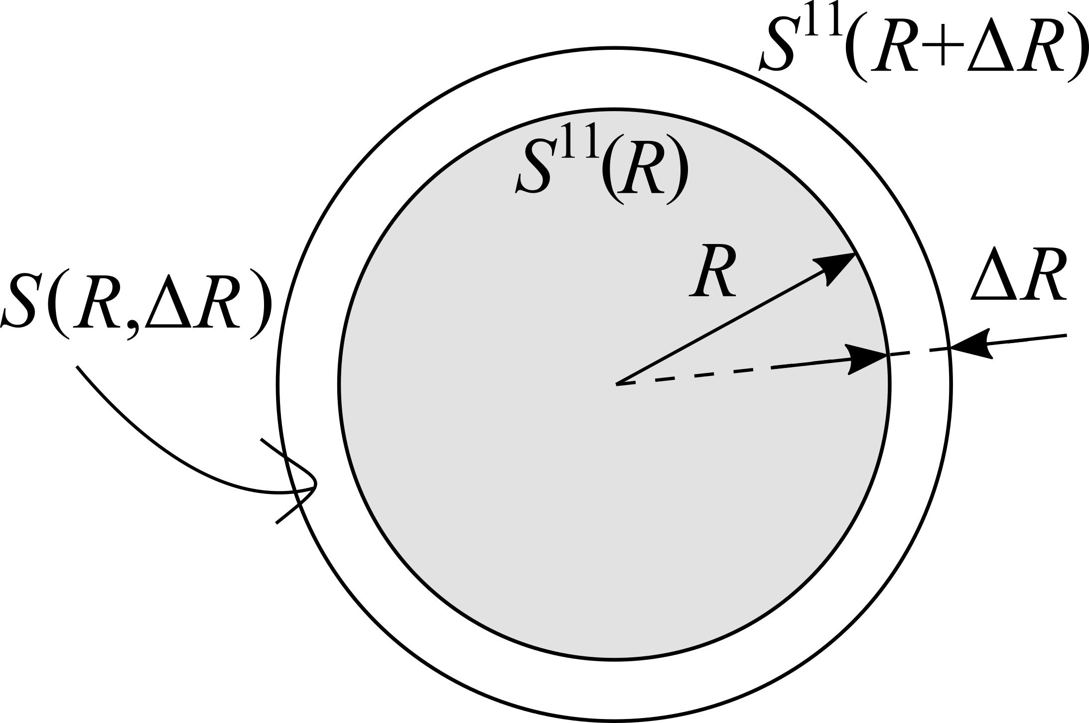
Figure 2: To the derivation of the scattering matrix algorithm.

A full calculation algorithm implementing Eq. (33) is also similar to what is described in [6]. Owing a homogeneous scattering particle with a continuous closed surface $\partial\Omega_{p}$ one should, first, choose a center of a spherical coordinate system, second, choose an inner and an outer spherical interfaces of radii $R_{in}$, $R_{out}$ centered at the origin, the first one being inscribed inside the particle, and the second one being circumscribed around it. The particle surface appears to be enclosed in the spherical layer. This partitioning is schematically shown in Fig. 3a,b. The permittivity inside the inscribed sphere is a constant being equal to the particle permittivity $\varepsilon_{p}$. Similarly, the permittivity of the region $r>R_{out}$ is the surrounding medium permittivity $\varepsilon_{m}$. The basis permittivity $\varepsilon_{b}$ to be ascribed to the region $R_{in}\leq r\leq R_{out}$ is essentially a free parameter of the method and is a matter of choice. Ideally it should not affect any physical quantities at the output of the method, and its influence on simulations and results will be discussed below.

A starting point of the algorithm is the diagonal matrix $S^{11}\left(R_{in}\right)$ filled with the Mie scattering coefficients obtained from the continuity boundary conditions at the interface $r=R_{in}$ separating media with permittivities $\varepsilon_{p}$ and $\varepsilon_{b}$ [22]. Explicitly,

$$\begin{array}[]{c}S_{nm}^{11,ee}\left(R_{in}\right)=\dfrac{j_{n}\left(k_{p}R_{in}\right)\tilde{j}_{n}\left(k_{b}R_{in}\right)-j_{n}\left(k_{b}R_{in}\right)\tilde{j}_{n}\left(k_{p}R_{in}\right)}{h_{n}^{(1)}\left(k_{b}R_{in}\right)\tilde{j}_{n}\left(k_{p}R_{in}\right)-j_{n}\left(k_{p}R_{in}\right)\tilde{h}_{n}^{(1)}\left(k_{b}R_{in}\right)}\\ S_{nm}^{11,hh}\left(R_{in}\right)=\dfrac{j_{n}\left(k_{p}R_{in}\right)\tilde{j}_{n}\left(k_{b}R_{in}\right)-\dfrac{\varepsilon_{b}}{\varepsilon_{p}}j_{n}\left(k_{b}R_{in}\right)\tilde{j}_{n}\left(k_{p}R_{in}\right)}{\dfrac{\varepsilon_{b}}{\varepsilon_{p}}h_{n}^{(1)}\left(k_{b}R_{in}\right)\tilde{j}_{n}\left(k_{p}R_{in}\right)-j_{n}\left(k_{p}R_{in}\right)\tilde{h}_{n}^{(1)}\left(k_{b}R_{in}\right)}\end{array}$$ (34)

and $S_{nm}^{11,eh}\left(R_{in}\right)=S_{nm}^{11,he}\left(R_{in}\right)=0$. Upper indices “$e$” and “$h$” correspond to the polarization of input and output waves, and $k_{p,b}=\omega\sqrt{\varepsilon_{p,b}\mu_{0}}$. Then, the layer $R_{in}<r<R_{out}$ of permittivity $\varepsilon_{b}$ should be divided into a number of thin shells, while the scattering matrix of each shell is explicitly given in Appendix A.

After $S^{11}$ matrix is accumulated by means of Eq. (33) for the increasing radial distance, a final multiplication by the scattering matrix of the spherical interface $r=R_{out}$ separating the basis and the outer medium should be made. To give this matrix explicitly we, first, fix the field decomposition in the vicinity of this interface. For $r=R_{out}-0$ this decomposition is the one used in all above derivations – into a superposition of regular and outgoing spherical waves (see Eq. (11)). For $r>R_{out}$ it is convenient to have the fields decomposed into a set of incoming and outgoing waves

$${\bf E}\left(\bm{r}\right)=\sum_{nm}\left[a_{nm}^{e}{\bf\mathcal{M}}{}_{nm}^{3}\left(k_{s}\bm{r}\right)+a_{nm}^{h}{\bf\mathcal{N}}_{nm}^{3}\left(k_{s}\bm{r}\right)+c_{nm}^{e}{\bf\mathcal{M}}_{nm}^{2}\left(k_{s}\bm{r}\right)+c_{nm}^{h}{\bf\mathcal{N}}_{nm}^{2}\left(k_{s}\bm{r}\right)\right],\thinspace r>R_{out}.$$ (35)

in order to define the incoming field via coefficients $c_{nm}^{e,h}$. Here $k_{s}=\omega\sqrt{\varepsilon_{s}\mu_{0}}$ is the wavenumber in the surrounding non-absorbing medium, and the upper index $"2"$ indicates that the corresponding spherical wave functions are written via the spherical Henkel functions of the second kind $z_{n}^{2}\equiv h_{n}^{(2)}$. Analogously to the Mie scattering scenario the boundary conditions yield a corresponding diagonal scattering matrix components. These components are specified in Appendix B.

7 Field solution in a basis spherical layer

Now let us return to the basis Eqs. (20)-(23) and use them for the self-consistent calculation of T-matrix single columns. In other words, for calculation of a response amplitude vector to a given excitation field. The basis equations now should be extended to yield a solution in the basis spherical layer $R_{in}\leq r\leq R_{out}$ taking into account multiple reflections at the layer interfaces (see Fig. 3b). Instead of constructing a corresponding Green’s tensor we will directly construct a field solution on the basis of the derived solution for the homogeneous space.

Let the reader recall the definition of the inner and the outer spherical interfaces bounding the scattering particle surface $\partial\Omega_{p}$, Fig. 3a, and put $R_{1}=R_{in}$, $R_{2}=R_{out}$ in (20)-(23). Then, the self-consistent field can be searched in form (e.g., see [17])

$$\begin{array}[]{c}\tilde{{\bf E}}\left(\bm{r}\right)=\sum_{nm}\left[C_{nm}^{ae}\tilde{a}_{nm}^{e}\left(R_{out}\right)+C_{nm}^{be}\tilde{b}_{nm}^{e}\left(R_{in}\right)\right]\mathcal{M}_{nm}^{1}\left(k_{p}\bm{r}\right)\\ +\left[C_{nm}^{ah}\tilde{a}_{nm}^{h}\left(R_{out}\right)+C_{nm}^{bh}\tilde{b}_{nm}^{h}\left(R_{in}\right)\right]\mathcal{N}_{nm}^{1}\left(k_{p}\bm{r}\right)\end{array}$$ (36)

for $r<R_{in}$,

$$\begin{array}[]{c}\tilde{{\bf E}}\left(\bm{r}\right)=\sum_{nm}\left[\tilde{a}_{nm}^{e}\left(r\right)+A_{nm}^{ae}\tilde{a}_{nm}^{e}\left(R_{out}\right)+A_{nm}^{be}\tilde{b}_{nm}^{e}\left(R_{in}\right)\right]\mathcal{M}_{nm}^{3}\left(k_{b}\bm{r}\right)\\ +\left[\tilde{a}_{nm}^{h}\left(r\right)+A_{nm}^{ah}\tilde{a}_{nm}^{h}\left(R_{out}\right)+A_{nm}^{bh}\tilde{b}_{nm}^{h}\left(R_{in}\right)\right]\mathcal{N}_{nm}^{3}\left(k_{b}\bm{r}\right)\\ +\left[\tilde{b}_{nm}^{e}\left(r\right)+B_{nm}^{ae}\tilde{a}_{nm}^{e}\left(R_{out}\right)+B_{nm}^{be}\tilde{b}_{nm}^{e}\left(R_{in}\right)\right]\mathcal{M}_{nm}^{1}\left(k_{b}\bm{r}\right)\\ +\left[\tilde{b}_{nm}^{h}\left(r\right)+B_{nm}^{ah}\tilde{a}_{nm}^{h}\left(R_{out}\right)+B_{nm}^{bh}\tilde{b}_{nm}^{h}\left(R_{in}\right)\right]\mathcal{N}_{nm}^{1}\left(k_{b}\bm{r}\right)\end{array}$$ (37)

for $R_{in}\leq r\leq R_{out}$, and

$$\begin{array}[]{c}\tilde{{\bf E}}\left(\bm{r}\right)=\sum_{nm}\left[D_{nm}^{ae}\tilde{a}_{nm}^{e}\left(R_{out}\right)+D_{nm}^{be}\tilde{b}_{nm}^{e}\left(R_{in}\right)\right]\mathcal{M}_{nm}^{3}\left(k_{m}\bm{r}\right)\\ +\left[D_{nm}^{ah}\tilde{a}_{nm}^{e}\left(R_{out}\right)+D_{nm}^{bh}\tilde{b}_{nm}^{e}\left(R_{in}\right)\right]\mathcal{N}_{nm}^{3}\left(k_{m}\bm{r}\right)\end{array}$$ (38)

for $r>R_{out}$. Similar expressions for the magnetic field follow directly from the first of Maxwell’s Eq. (3) and transformation relations (8). Note, that according to (20)-(23) $\tilde{a}_{nm}^{e,h}\left(R_{in}\right)=\tilde{b}_{nm}^{e,h}\left(R_{out}\right)=0$. The external field here is no more the field of the homogeneous space, but rather the self-consistent field of the spherical particle of radius $r=R_{in}$ and permittivity $\varepsilon_{p}$ covered by the spherical layer $R_{in}\leq r\leq R_{out}$ of permittivity $\varepsilon_{b}$, and placed in the medium of permittivity $\varepsilon_{s}$.

Unknown sets of coefficients $A$, $B$, $C$, and $D$ are found from the continuity of the tangential field components at the interfaces $r=R_{in},R_{out}$ analogously to the Mie theory and derivations of Appendix B. They can be expressed via the S-matrices of the inner and the outer interfaces introduced within the scattering matrix algorithm (see Eq. (34) and Appendix B). The resulting formulas explicitly write

$$A_{nm}^{a\star}\tilde{a}_{nm}^{\star}\left(R_{out}\right)+A_{nm}^{b\star}\tilde{b}_{nm}^{\star}\left(R_{in}\right)=S_{nm}^{11,\star\star}\left(R_{in}\right)\frac{S_{nm}^{22,\star\star}\left(R_{out}\right)\tilde{a}_{nm}^{\star}\left(R_{out}\right)+\tilde{b}_{nm}^{\star}\left(R_{in}\right)}{1-S_{nm}^{11,\star\star}\left(R_{in}\right)S_{nm}^{22,\star\star}\left(R_{out}\right)}$$ (39)

$$B_{nm}^{a\star}\tilde{a}_{nm}^{\star}\left(R_{out}\right)+B_{nm}^{b\star}\tilde{b}_{nm}^{\star}\left(R_{in}\right)=S_{nm}^{22,\star\star}\left(R_{out}\right)\frac{\tilde{a}_{nm}^{\star}\left(R_{out}\right)+S_{nm}^{11,\star\star}\left(R_{in}\right)\tilde{b}_{nm}^{\star}\left(R_{in}\right)}{1-S_{nm}^{11,\star\star}\left(R_{in}\right)S_{nm}^{22,\star\star}\left(R_{out}\right)}$$ (40)

$$C_{nm}^{a\ast}\tilde{a}_{nm}^{\star}\left(R_{out}\right)+C_{nm}^{b\star}\tilde{b}_{nm}^{\star}\left(R_{in}\right)=S_{nm}^{21,\star\star}\left(R_{in}\right)\frac{S_{nm}^{22,\star\star}\left(R_{out}\right)\tilde{a}_{nm}^{\star}\left(R_{out}\right)+\tilde{b}_{nm}^{\star}\left(R_{in}\right)}{1-S_{nm}^{11,\star\star}\left(R_{in}\right)S_{nm}^{22,\star\star}\left(R_{out}\right)}$$ (41)

$$D_{nm}^{a\star}\tilde{a}_{nm}^{\star}\left(R_{out}\right)+D_{nm}^{b\star}\tilde{b}_{nm}^{\star}\left(R_{in}\right)=S_{nm}^{12,\star\star}\left(R_{out}\right)\frac{S_{nm}^{22,\star\star}\left(R_{out}\right)\tilde{a}_{nm}^{\star}\left(R_{out}\right)+\tilde{b}_{nm}^{\star}\left(R_{in}\right)}{1-S_{nm}^{11,\star\star}\left(R_{in}\right)S_{nm}^{22,\star\star}\left(R_{out}\right)}$$ (42)

where the star $\star$ can be either “$e$”, or “$h$”. Also used here the transmission coefficients of the inner interface are

$$\begin{array}[]{c}S_{nm}^{21,ee}\left(R_{in}\right)=\dfrac{i}{k_{b}R_{in}}\dfrac{1}{j_{n}\left(k_{p}R_{in}\right)\tilde{h}_{n}^{(1)}\left(k_{b}R_{in}\right)-h_{n}^{(1)}\left(k_{b}R_{in}\right)\tilde{j}_{n}\left(k_{p}R_{in}\right)}\\ S_{nm}^{21,hh}\left(R_{in}\right)=\dfrac{i}{k_{p}R_{in}}\dfrac{1}{j_{n}\left(k_{p}R_{in}\right)\tilde{h}_{n}^{(1)}\left(k_{b}R_{in}\right)-\dfrac{\varepsilon_{b}}{\varepsilon_{p}}h_{n}^{(1)}\left(k_{b}R_{in}\right)\tilde{j}_{n}\left(k_{p}R_{in}\right)}\end{array}$$ (43)

Eqs. (36)-(38) with coefficients (39)-(42) and radially dependent amplitudes $\tilde{a}_{nm}^{e,h}\left(r\right)$, $\tilde{b}_{nm}^{e,h}\left(r\right)$ defined by Eqs. (20)-(23) are the solution sought in the case of the spherical layer basis medium.

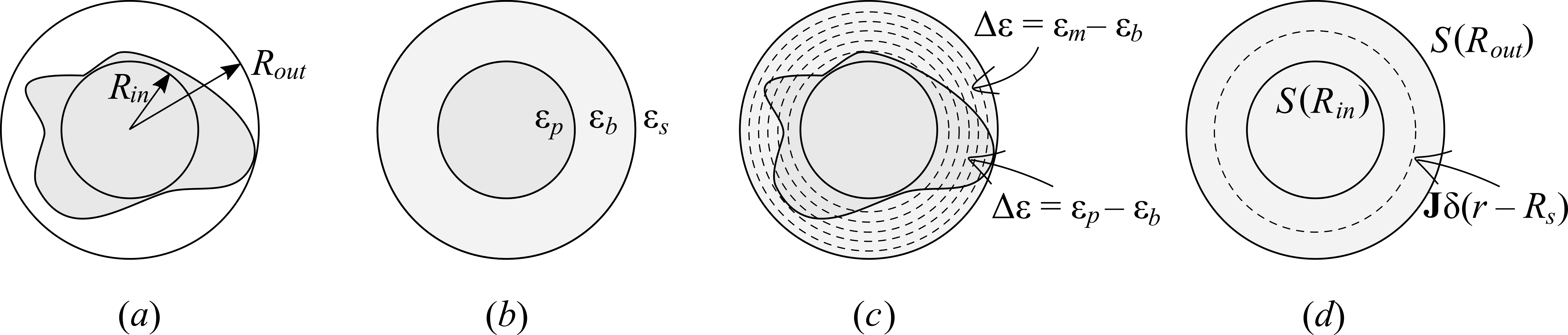
Figure 3: Illustrations to the scattering matrix and the scattering vector algorithms. a) inscribed and ascribed spherical surfaces; b) basis medium for the scattering vector algorithm consisting of a core of a permittivity equal to the particle permittivity, a spherical layer of a permittivity being a free parameter of the methods, and a surrounding medium; c) slicing of the basis layer into a set of thin spherical shells; d) a radial “delta”-source located inside the basis layer.

It might be interesting to note that Eqs. (39)-(42) can be derived with the aids of considerations similar to those given while developing the scattering matrix algorithm in the previous section. Consider a spherical layer (Fig. …) $R_{in}\leq r\leq R_{out}$ together with the volume “delta”-source inside ${\bf J}=\delta(r-R_{s}){\bf J}\left(\theta,\varphi\right)$, $R_{in}<R_{s}<R_{out}$. Let the field emitted by the source be decomposed into the spherical vector waves having amplitude vectors $\bm{b_{J}}$ for $r<R_{s}$ (being regular wave functions), and $\bm{a_{J}}$ for $r>R_{s}$ (being outgoing wave functions). These are amplitudes which the source would emit in the absence of the interfaces $r=R_{in,out}$. To find self-consistent amplitudes in the presence of the interfaces let us use the S-matrix relations at both interfaces $S\left(R_{in,out}\right)$:

$$\begin{array}[]{c}\bm{b}=\bm{b_{J}}+S^{11}\left(R_{out}\right)\bm{a}\\ \bm{a}=\bm{a_{J}}+S^{22}\left(R_{in}\right)\bm{b}\end{array}$$ (44)

where $\bm{a}$ and $\bm{b}$ are unknown amplitude vectors of the self-consistent filed inside the layer. Solution of these equations is

$$\begin{array}[]{c}\bm{b}=\bm{b_{J}}+S^{11}\left(R_{out}\right)\left[I-S^{22}\left(R_{in}\right)S^{11}\left(R_{out}\right)\right]^{-1}\left[\bm{a_{J}}+S^{22}\left(R_{in}\right)\bm{b_{J}}\right]\\ \bm{a}=\bm{a_{J}}+S^{22}\left(R_{in}\right)\left[I-S^{11}\left(R_{out}\right)S^{22}\left(R_{in}\right)\right]^{-1}\left[\bm{b_{J}}+S^{11}\left(R_{out}\right)\bm{a_{J}}\right]\end{array}$$ (45)

Bearing in mind the fact that scattering matrices of spherical interfaces are diagonal, Eqs. (45) immediately become (39), (40). Amplitude vectors inside the sphere $r<R_{1}$, and in the outer space $r>R_{2}$ are found via S-matrix relations on the basis of this self-consistent field as $\bm{b}|_{r<R_{1}}=S^{21}\left(R_{in}\right)\bm{b}$, $\bm{a}|_{r>R_{2}}=S^{12}\left(R_{out}\right)\bm{b}$.

8 Scattering vector algorithm

To solve the equations derived in the previous section the spherical layer should be divided into $N_{s}$ thin spherical shells of thickness $\Delta R=\left(R_{out}-R_{in}\right)/N_{s}$ (Fig. 3c) to approximate the integration by finite sums (here the mid-point rule is applied). Upon truncation of infinite series of the spherical wave functions one runs into a finite self-consistent linear equation system on unknown field amplitudes. This system can be written as follows:

$$\bm{V}=\left({\bf I}-\mathcal{P}\mathcal{R}\right)^{-1}\bm{V}^{inc}$$ (46)

where vectors $\bm{V}$, $\bm{V}^{inc}$ contain unknown and incident amplitudes in all shells $\tilde{a}_{nm,k}^{e,h}=\tilde{a}_{nm}^{e,h}\left(r_{k}\right)$, $\tilde{b}_{nm,k}^{e,h}=\tilde{b}_{nm}^{e,h}\left(r_{k}\right)$, $r_{k}=R_{in}+\left(k+1/2\right)\Delta R$, $k=0,\thinspace 1,\thinspace\dots,\thinspace N_{s}-1$. Matrix operator $\mathcal{R}$ describes the scattering in each thin shell. It is diagonal relative to the index $k$ enumerating shells, and explicitly is given by Eq. (30) with S-matrix components listed in Appendix A. The second operator $\mathcal{P}$ corresponds to propagation of the vector spherical waves between different shells, and implies the weighted summation of the output of the operator $\mathcal{R}$ in accordance with Eqs. (36)-(38). This summation can be organized with two loops, so that the resulting algorithm can be formulated as follows:

1. Choose the truncation number for spherical harmonics $N=\max n$, and pre-calculate coefficient matrices $A$, $B$, $C$, and $D$ on the basis of Eqs. (39)-(42).

2. Choose a basis layer, its subdivision into shells, and calculate spherical harmonic transformation of the permittivity, Eq. (19), in each shell. Pre-calculate S-matrix components for all shells on the basis of Eqs. (24), (25), and Appendix A.

3. Solve Eq. (46) by means of an iterative method like the Bi-conjugate Gradient or the Generalized Minimal Residual method. At each iteration step do the following:

   1. multiply amplitudes in each shell by the corresponding scattering matrices in accordance with Eq. (30) and Appendix A.

   2. loop over shells and store the partial sums for each shell: $\tilde{\bm{a}}_{nm,k}^{sum}=\sum_{j=0}^{k}\tilde{\bm{a}}_{nm,j}$, $\tilde{\bm{b}}_{nm,k}^{sum}=\sum_{j=k}^{N_{s}-1}\tilde{\bm{b}}_{nm,j}$. Then the accumulated amplitudes $\tilde{\bm{a}}_{nm,N_{s}-1}^{sum}$ and $\tilde{\bm{b}}_{nm,0}^{sum}$ should be multiplied by the weight factors according to Eqs. (39)-(42) and added to the stored amplitudes in each shell as Eq. (37) requires.

9 Implementation details

The described methods were implemented in C++ and compiled under Windows using the MS Visual Studio compiler. In particular, spherical Bessel functions are calculated on the basis of [23], associated Legendre polynomials – on the basis of [24], Clebsch-Gordan coefficients – on the basis of [25]. An important feature of the referenced algorithms is that they allow calculating whole sets of required functions for one of their indices at a single iteration cycle, which substantially saves computation time. Both the scattering matrix and the scattering vector algorithms require evaluation of factors in Eqs. (25), which do not depend on a particular permittivity function and on radial distance. Namely, matrices

$$\begin{array}[]{c}\hat{Q}_{nm;pq,u}^{r}=\dfrac{\left(-1\right)^{q}}{\sqrt{2}}\sqrt{2n+1}\sqrt{2p+1}\dfrac{C_{p,q;n,-m}^{u,m-q}C_{p,0;n,0}^{u,0}}{\sqrt{2u+1}}\\ \hat{Q}_{nm;pq,u}^{\pm}=\dfrac{\left(-1\right)^{q}}{\sqrt{2}}\sqrt{2n+1}\sqrt{2p+1}\dfrac{C_{p,q;n,-m}^{u,m-q}C_{p,1;n,-1}^{u,0}}{\sqrt{2u+1}}\end{array}$$ (47)

are pre-calculated, stored, and then used for finding the scattering matrix elements in each shell. In case of large-scale computations it seems to be reasonable to create a library of matrix elements (47) for them to be readily available. Within the scattering vector algorithm vectors (24), transmission and reflection coefficients for the inner and the outer spherical interfaces are also pre-calculated.

The following examples concern scattering by spheroids, and general polyhedral particles. The spheroidal shape particles with the axis of revolution coinciding with the coordinate axis $Z$ allow for analytic formulas for the spherical harmonic decomposition of the dielectric function:

$$\left[\mathcal{E}\right]_{nm}\left(r\right) =\frac{1}{2\pi}\intop_{0}^{\pi}\mathcal{E}\left(r,\theta\right)P_{n}^{m}\left(\theta\right)\sin\theta d\theta\intop_{0}^{2\pi}\exp\left(-im\varphi\right)d\varphi$$

$$=\delta_{m0}\mathcal{E}_{1}\left[\intop_{0}^{\Theta\left(r\right)}P_{n}\left(\theta\right)\sin\theta d\theta+\intop_{\pi-\Theta\left(r\right)}^{\pi}P_{n}\left(\theta\right)\sin\theta d\theta\right]+\delta_{m0}\mathcal{E}_{2}\intop_{\Theta\left(r\right)}^{\pi-\Theta\left(r\right)}P_{n}\left(\theta\right)\sin\theta d\theta$$ (48)

$$=\delta_{m0}\left\{\sqrt{2}\delta_{n0}\mathcal{E}_{1}+\delta_{n,2k}\left(\mathcal{E}_{2}-\mathcal{E}_{1}\right)\dfrac{1}{\sqrt{4k+1}}\left[\dfrac{P_{2k+1}\left(\Theta\right)}{\sqrt{4k+3}}-\dfrac{P_{2k-1}\left(\Theta\right)}{\sqrt{4k-1}}\right]\right\}$$

Symbol $\mathcal{E}$ stands for any of functions in (19). Due to the inner summation in Eqs. (25) decompositions of the permittivity functions into the spherical harmonics should be done for twice larger maximum harmonic degree $2N$ than the one used in the methods. Functions (47) are also simplified since indices $m=q$ (for further simplification of the method based on the rotational symmetry, see [11]).

In case of a general polyhedron particle the following approach can be applied (see Fig. 4 for illustration). First, the integration over the polar angle $\theta$ has to be replaced with the Gaussian quadrature summation characterized by weights $w_{j}$ and angles $\theta_{j}$, $j=1,\dots,N_{\theta}$. Note that a uniform series expansion for an iteration-free calculation of the Gauss-Legendre nodes and weights provided by [26], and used here, allows for an efficient computation even of highly oscillating integrals at high precision. Second, given a thin spherical shell of central radius $R_{k}$, intersections of the sphere of the same radius with cones $\theta=\theta_{j}$ yield a set of circles. In turn, being intersected with the polyhedron each circle appears to be divided into an even number of arcs described by azimuthal angles $\varphi_{jl}\left(R_{k}\right)$. Each of these arcs lies either inside the polyhedron, and corresponds to some constant $\mathcal{E}_{in}$, or outside the polyhedron, and corresponds to another constant $\mathcal{E}_{out}$. Therefore, the integration over the azimuthal angle can be done analytically, and the whole decomposition becomes

$$\left[\mathcal{E}\right]_{nm}\left(R_{k}\right) \approx\frac{1}{2\pi}\sum_{j=0}^{N_{\theta}-1}w_{j}P_{n}^{m}\left(\theta_{j}\right)\sin\theta_{j}\left[\mathcal{E}_{in}\sum_{j}\intop_{\varphi_{jl}}^{\varphi_{jl+1}}\exp\left(-im\varphi\right)d\varphi+\mathcal{E}_{out}\sum_{j}\intop_{\varphi_{jl+1}}^{\varphi_{jl+2}}\exp\left(-im\varphi\right)d\varphi\right]$$

$$=\sqrt{2}\mathcal{E}_{out}\delta_{m0}\delta_{n0}+\frac{\mathcal{E}_{in}-\mathcal{E}_{out}}{2\pi}\sum_{j=0}^{N_{\theta}-1}w_{j}P_{n}^{m}\left(\theta_{j}\right)\sin\theta_{j}\sum_{l}\Delta\varphi_{jl}{\rm sinc}\left(\frac{1}{2}m\Delta\varphi_{jl}\right)\exp\left[-\frac{1}{2}im\left(\varphi_{jl+1}+\varphi_{jl}\right)\right]$$ (49)

where $\Delta\varphi_{jl}=\varphi_{jl+1}-\varphi_{jl}$. For numerical evaluation of Eq. (49) values of $P_{n}^{m}\left(\theta_{j}\right)$ can be pre-calculated, and then calculation of $\left[\mathcal{E}\right]_{nm}\left(R_{k}\right)$ can be done in parallel for a given set of shells.

Figure 4: Illustration to the algorithm of the spherical harmonic transformation of a polyhedron-sphere intersection.

When using either the scattering matrix or the scattering vector approaches it is also preferable to benefit from the fact that solutions should converge polynomially relative to increasing maximum degree of spherical harmonics $N$ and the number of spherical shells $N_{s}$ used within the discretization procedures. When such convergence is not significantly perturbed by numerical errors, one can

10 Numerical properties

Accuracy of solutions of both the scattering matrix and the scattering vector methods depends primarily on the number of spherical shells $N_{s}$ and the maximum degree $N$ of spherical harmonic decomposition. To attain accurate solutions of scattering problems the analysis is done here in two steps. First, for fixed $N$ one looks for a limit at increasing $N_{s}$, which corresponds to evaluation of integrals in Eqs. (20)-(23). Second, given the converged solutions for several values of $N$ the convergence relative this truncation number is traced. It was found that for fixed values of $N$ convergence curves corresponding to increasing $N_{s}$ are all pretty similar. Fig. 5 demonstrates an example of such convergence for the scattering matrix method for a prolate spheroid of equatorial size parameter $kd=10$, semi-axes ratio equal to $a/b=5$ and permittivity $\varepsilon_{p}=4$. The vertical axis shows the maximum absolute difference between scattering matrix components corresponding to subsequent values of $N_{s}$. The rate of convergence is polynomial as follows theoretically from the used integration rules, and this rate can be substantially improved by the Richardson extrapolation. This is shown by the two lower curves in Fig. 5 corresponding to the first and the second order extrapolation. Fig. 6 demonstrates the accuracy of the energy conservation law (power balance – relation between incident and scattered power minus 1) corresponding to the calculated and extrapolated solutions of Fig. 5. The solutions converged relative to $N_{s}$ are then taken to trace the convergence for increasing $N$ (the accuracy of radial integral evaluation should be enough not to affect this latter convergence). Dependence of maximum absolute difference between corresponding scattering matrix components for a prolate spheroid of $kd=4$, $a/b=2$, and $\varepsilon_{p}=2$ is shown in Fig 7.

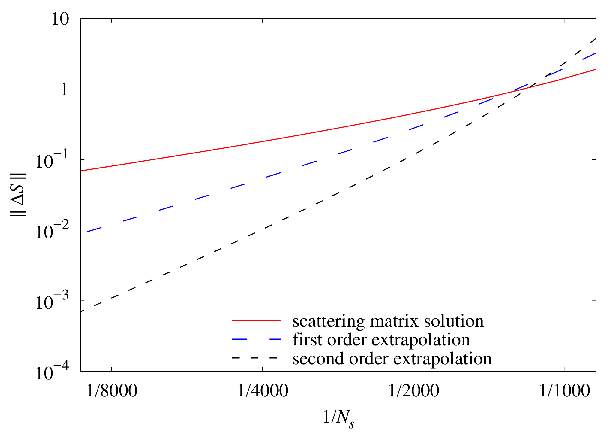
Figure 5: Convergence of the scattering matrix calculated by the scattering matrix method for increasing number of spherical shells $N_{s}$ and fixed spherical harmonic degree truncation number $N$ (the graphs for different values of $N$ are pretty similar) in case of scattering by a prolate spheroidal particle of equatorial size parameter $kd=10$, semi-axes ratio $a/b=5$ and permittivity $\varepsilon_{p}=4$.

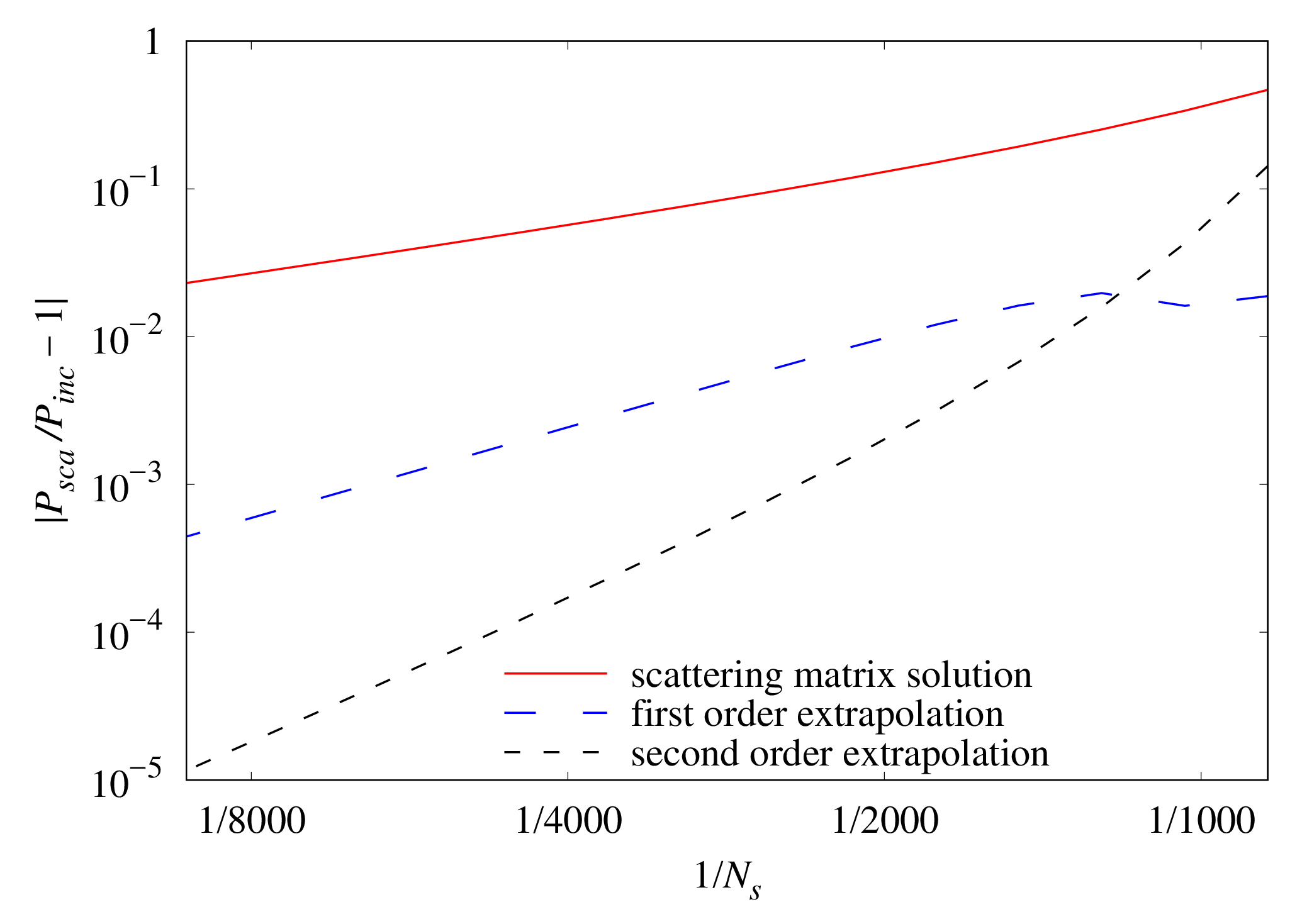
Figure 6: Power balance of the solutions attained by the scattering matrix method and corresponding to the convergence shown in Fig. 5.

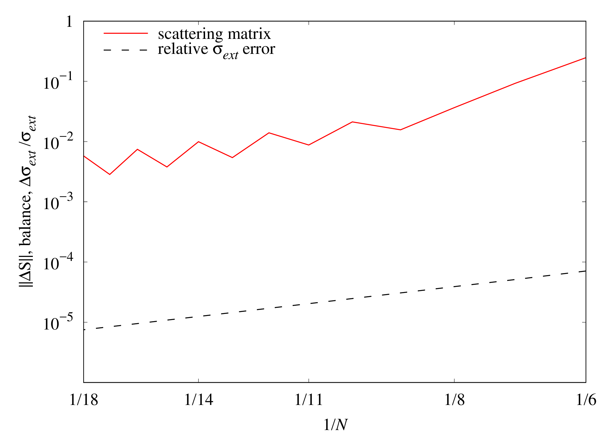
Figure 7: Convergence of the scattering matrix, and relative extinction cross section calculated by the scattering matrix method for increasing number of spherical harmonic degree truncation number $N$ providing that each calculated matrix is converged over $N_{s}$ up to a sufficient precision. This example is for scattering by prolate spheroidal particle of equatorial size parameter $kd=4$, semi-axes ratio $a/b=2$ and permittivity $\varepsilon_{p}=2$.

Figs. 8–10 demonstrate the same convergence plots as Figs. 5–7 for the scattering vector method based calculations. This method has the second order polynomial convergence rate relative to increasing $N_{s}$, so only the second order Richardson extrapolation is applied here. Importantly, one can also notice that calculated scattering vector solutions have almost zero power balance contrary to the scattering matrix method, Fig. 6.

An example of a complex shape polyhedral particles was generated by randomly shifting and stretching of icosahedron vertex positions. Fig. 11 demonstrates an example of such a particle, which has no symmetries, and Fig. 12 shows the convergence of the scattering vector method applied to such particle with characteristic size (circumscribed sphere diameter) $kD=8$ and permittivity 2.

Free parameter $\varepsilon_{b}$ fairly affects the results of the scattering matrix method when being chosen to be pure real and to vary within the interval $\varepsilon_{s}\leq\varepsilon_{b}\leq\text{$\Re\varepsilon_{p}$}$. On the opposite, this parameter may slightly affect the convergence speed of a linear solver of the equation system (46) being for example the GMRes or the BiCGstab. This convergence was also found not only to depend predictably on the refractive index contrast and the size parameter, but to increase with the increasing number $N$, which may probably be related to a loss of accuracy. Viz, for a given scattering particle the number of iterations $n_{it}$ required to solve the system (46) is independent of $N$ for relatively small $N$ but at some point starts to substantially increase. Amid this effect the stagnation of the iterative process occurs. To overcome these barriers and to gain the most of the parallelization potential of the scattering vector algorithm it seems to be essential to search for a suitable preconditioner which is a subject of a future research.

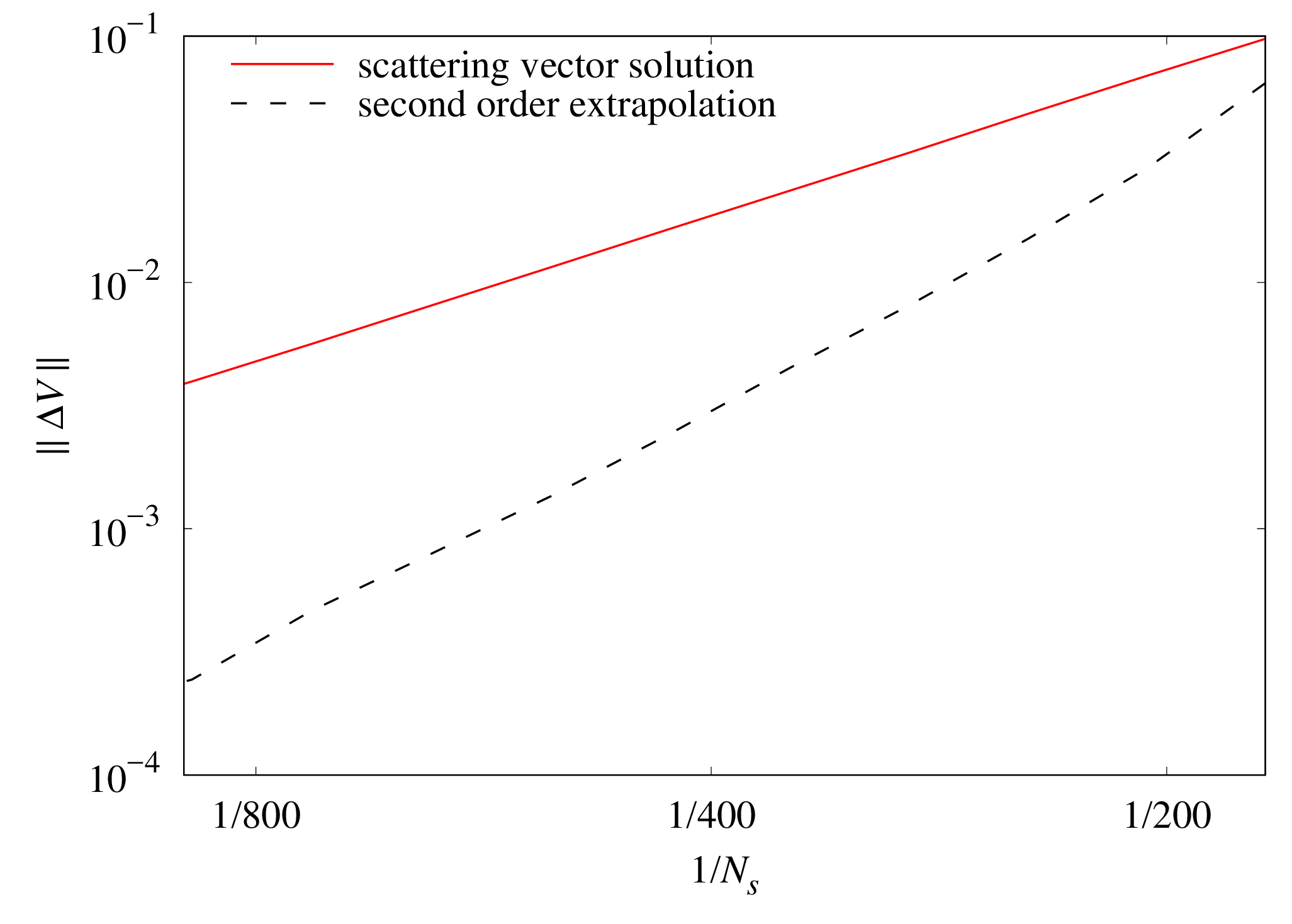
Figure 8: Same as in Fig. 5, but for the scattering vector method.

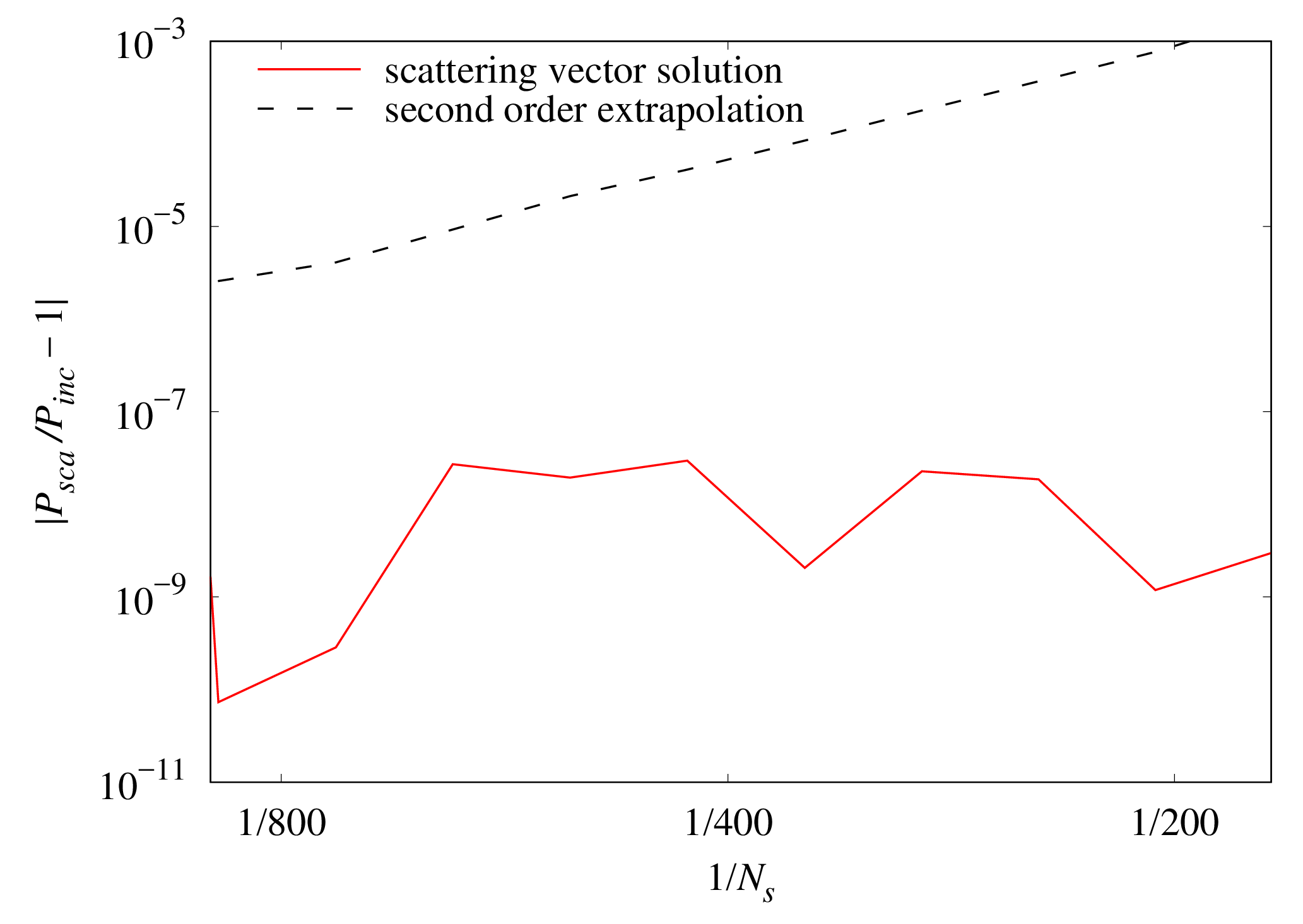
Figure 9: Same as in Fig. 6, but for the scattering vector method.

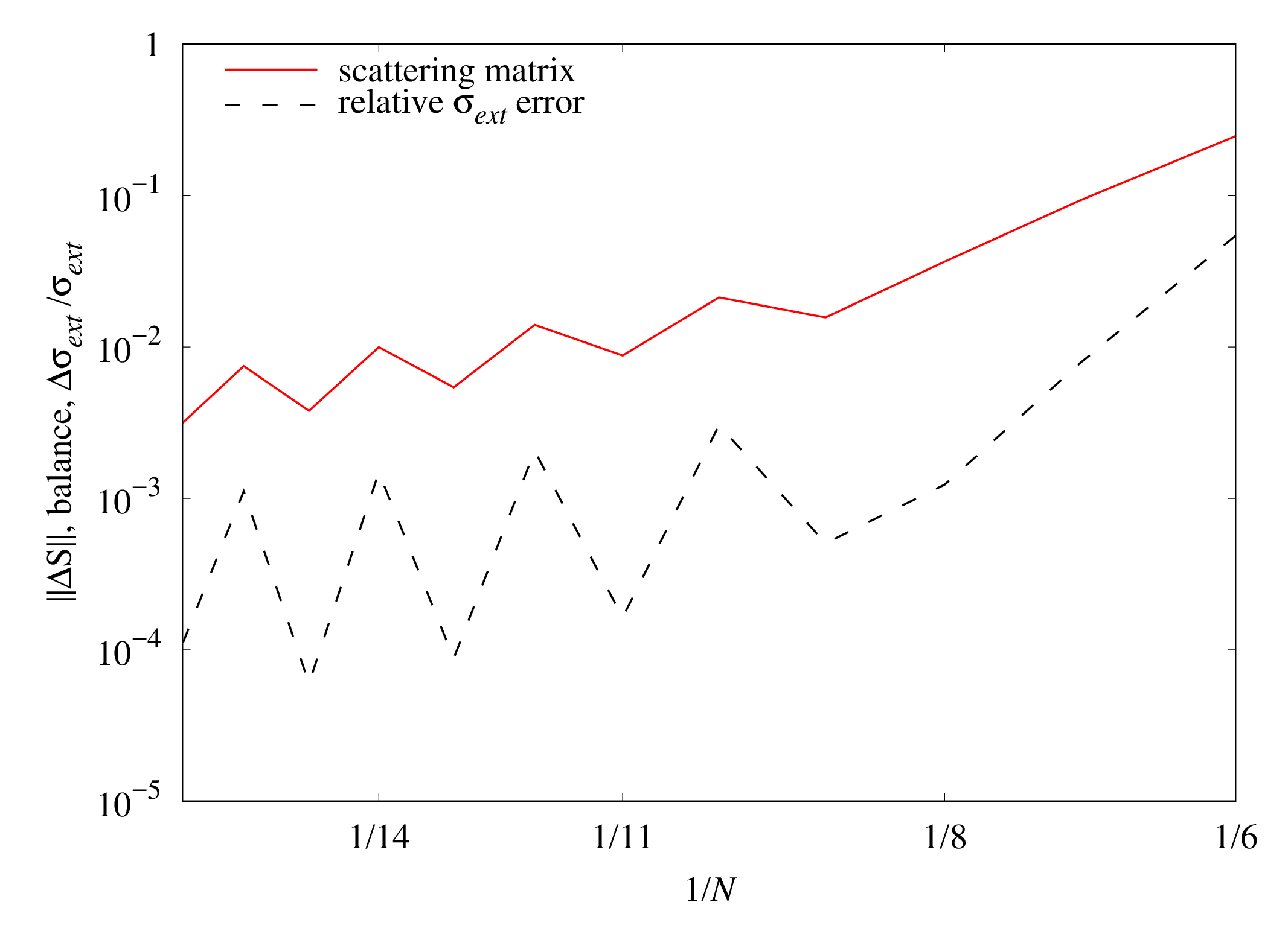
Figure 10: Same as in Fig. 7, but for the scattering vector method.

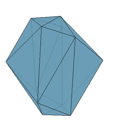
Figure 11: Example of a scattering particle of irregular shape. The particle is generated by randomly shifting positions of vertices of a regular icosahedron.

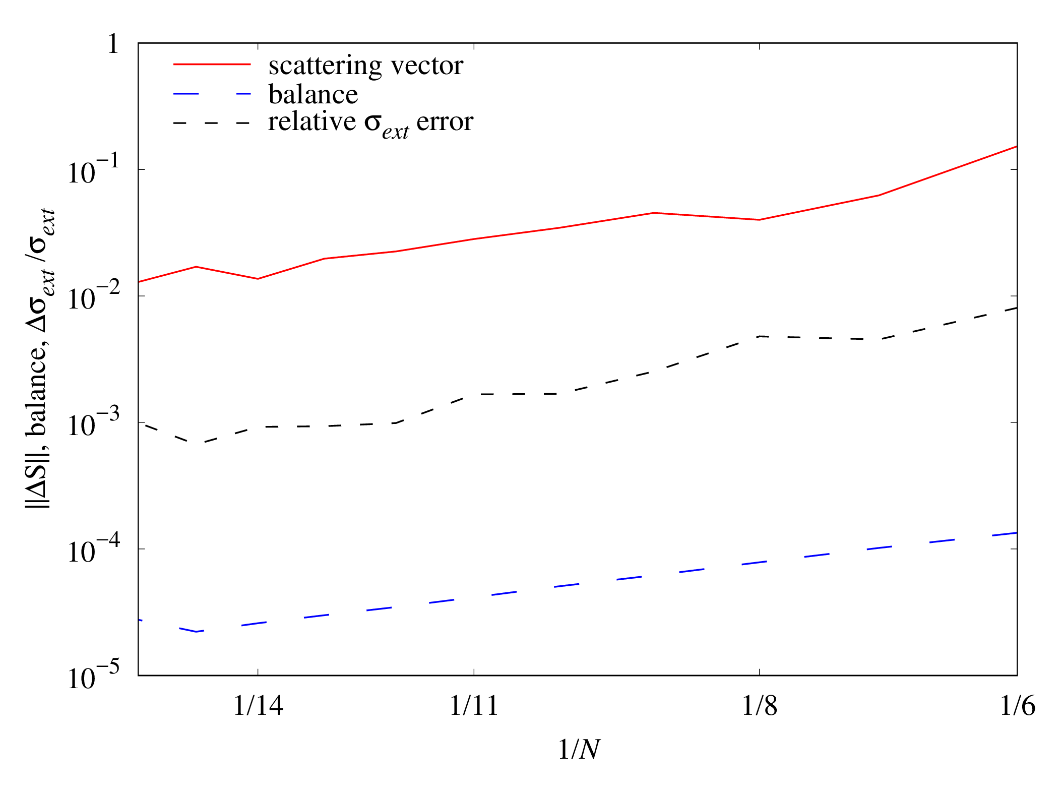
Figure 12: Convergence of the scattering matrix, power balance and the relative extinction cross section calculated by the scattering matrix method for increasing number of spherical harmonic degree truncation number $N$ providing that each calculated matrix is converged over $N_{s}$ up to a sufficient precision. This example is for scattering by an irregular polyhedral particle of size parameter $kd=8$, and permittivity $\varepsilon_{p}=2$.

11 Summary

To conclude, the work provides the derivation of a method analogous to the IIM on the basis of the Generalized Source approach. In analogy with the planar geometry case the method is referred to as the scattering matrix method. The Generalized Source viewpoint will allow to extend the approach to the curvilinear coordinate transformations and related metric sources in a next publication. Simultaneously an alternative to the scattering matrix method, the method of calculating separate scattering matrix columns – the scattering vector method, is developed. The latter method relies on the iterative solution of linear equation systems and adopts parallelization which makes it potentially attractive for large scale computations, though an additional work to improve its numerical behavior is required. It is shown that the scattering vector method yields solutions with almost zero power balance when applied to dielectric particles. In addition the paper proposes an algorithm of computing of spherical harmonic transformations for cross-sections coming from crossing of arbitrary polyhedral shape scattering particles by thin spherical shells.

Appendix A

This appendix lists the explicit components of the scattering matrix present in Eq. (30)

$$S_{nm,pq}^{11,ee}\left(x,\Delta x\right)=i\Delta x{\bf\mathcal{V}}_{n1}^{(1)}\left(x\right)Q_{nm,pq}^{+}\left(x\right){\bf\mathcal{V}}_{p1}^{(1)}\left(x\right)$$ (50)

$$S_{nm,pq}^{11,eh}\left(x,\Delta x\right)=i\Delta x{\bf\mathcal{V}}_{n1}^{(1)}\left(x\right)Q_{nm,pq}^{-}\left(x\right){\bf\mathcal{V}}_{p2}^{(1)}\left(x\right)$$ (51)

$$S_{nm,pq}^{11,he}\left(x,\Delta x\right)=-i\Delta x{\bf\mathcal{V}}_{n2}^{(1)}\left(x\right)Q_{nm,pq}^{-}\left(x\right){\bf\mathcal{V}}_{p1}^{(1)}\left(x\right)$$ (52)

$$S_{nm,pq}^{11,hh}\left(x,\Delta x\right)=i\Delta x\left[{\bf\mathcal{V}}_{n3}^{(1)}\left(x\right)Q_{nm,pq}^{r}\left(x\right){\bf\mathcal{V}}_{p3}^{(1)}\left(x\right)-{\bf\mathcal{V}}_{n2}^{(1)}\left(x\right)Q_{nm,pq}^{+}\left(x\right){\bf\mathcal{V}}_{p2}^{(1)}\left(x\right)\right]$$ (53)

$$S_{nm,pq}^{12,ee}\left(x,\Delta x\right)=1+i\Delta x{\bf\mathcal{V}}_{n1}^{(1)}\left(x\right)Q_{nm,pq}^{+}\left(x\right){\bf\mathcal{V}}_{p1}^{(3)}\left(x\right)$$ (54)

$$S_{nm,pq}^{12,eh}\left(x,\Delta x\right)=i\Delta x{\bf\mathcal{V}}_{n1}^{(1)}\left(x\right)Q_{nm,pq}^{-}\left(x\right){\bf\mathcal{V}}_{p2}^{(1)}\left(x\right)$$ (55)

$$S_{nm,pq}^{12,he}\left(x,\Delta x\right)=-i\Delta x{\bf\mathcal{V}}_{n2}^{(1)}\left(x\right)Q_{nm,pq}^{-}\left(x\right){\bf\mathcal{V}}_{p1}^{(3)}\left(x\right)$$ (56)

$$S_{nm,pq}^{12,hh}\left(x,\Delta x\right)=1+i\Delta x\left[{\bf\mathcal{V}}_{n3}^{(1)}\left(x\right)Q_{nm,pq}^{r}\left(x\right){\bf\mathcal{V}}_{p3}^{(3)}\left(x\right)-{\bf\mathcal{V}}_{n2}^{(1)}\left(x\right)Q_{nm,pq}^{+}\left(x\right){\bf\mathcal{V}}_{p2}^{(3)}\left(x\right)\right]$$ (57)

$$S_{nm,pq}^{21,ee}\left(x,\Delta x\right)=1+i\Delta x{\bf\mathcal{V}}_{n1}^{(3)}\left(x\right)Q_{nm,pq}^{+}\left(x\right){\bf\mathcal{V}}_{p1}^{(1)}\left(x\right)$$ (58)

$$S_{nm,pq}^{21,eh}\left(x,\Delta x\right)=i\Delta x{\bf\mathcal{V}}_{n1}^{(3)}\left(x\right)Q_{nm,pq}^{-}\left(x\right){\bf\mathcal{V}}_{p2}^{(1)}\left(x\right)$$ (59)

$$S_{nm,pq}^{21,he}\left(x,\Delta x\right)=-i\Delta x{\bf\mathcal{V}}_{n2}^{(3)}\left(x\right)Q_{nm,pq}^{-}\left(x\right){\bf\mathcal{V}}_{p1}^{(1)}\left(x\right)$$ (60)

$$S_{nm,pq}^{21,hh}\left(x,\Delta x\right)=1+i\Delta x\left[{\bf\mathcal{V}}_{n3}^{(3)}\left(x\right)Q_{nm,pq}^{r}\left(x\right){\bf\mathcal{V}}_{p3}^{(1)}\left(x\right)-{\bf\mathcal{V}}_{n2}^{(3)}\left(x\right)Q_{nm,pq}^{+}\left(x\right){\bf\mathcal{V}}_{p2}^{(1)}\left(x\right)\right]$$ (61)

$$S_{nm,pq}^{22,ee}\left(x,\Delta x\right)=i\Delta x{\bf\mathcal{V}}_{n1}^{(3)}\left(x\right)Q_{nm,pq}^{+}\left(x\right){\bf\mathcal{V}}_{p1}^{(3)}\left(x\right)$$ (62)

$$S_{nm,pq}^{22,eh}\left(x,\Delta x\right)=i\Delta x{\bf\mathcal{V}}_{n1}^{(3)}\left(x\right)Q_{nm,pq}^{-}\left(x\right){\bf\mathcal{V}}_{p2}^{(1)}\left(x\right)$$ (63)

$$S_{nm,pq}^{22,he}\left(x,\Delta x\right)=-i\Delta x{\bf\mathcal{V}}_{n2}^{(3)}\left(x\right)Q_{nm,pq}^{-}\left(x\right){\bf\mathcal{V}}_{p1}^{(3)}\left(x\right)$$ (64)

$$S_{nm,pq}^{22,hh}\left(x,\Delta x\right)=i\Delta x\left[{\bf\mathcal{V}}_{n3}^{(3)}\left(x\right)Q_{nm,pq}^{r}\left(x\right){\bf\mathcal{V}}_{p3}^{(3)}\left(x\right)-{\bf\mathcal{V}}_{n2}^{(3)}\left(x\right)Q_{nm,pq}^{+}\left(x\right){\bf\mathcal{V}}_{p2}^{(3)}\left(x\right)\right]$$ (65)

Multiplication of the amplitude vector $\left(\tilde{a}_{nm}^{e}\left(x\right),\thinspace\tilde{b}_{nm}^{e}\left(x\right),\thinspace\tilde{a}_{nm}^{h}\left(x\right),\thinspace\tilde{b}_{nm}^{h}\left(x\right)\right)^{T}$ by this matrix can be performed in the following three steps:

1. Calculate intermediate coefficient vectors

   $$\begin{array}[]{c}\xi_{nm}^{1}\left(x\right)={\bf\mathcal{V}}_{n1}^{(3)}\left(x\right)\tilde{a}_{nm}^{e}\left(x\right)+{\bf\mathcal{V}}_{n1}^{(1)}\left(x\right)\tilde{b}_{nm}^{e}\left(x\right)\\ \xi_{nm}^{2}\left(x\right)={\bf\mathcal{V}}_{n2}^{(3)}\left(x\right)\tilde{a}_{nm}^{h}\left(x\right)+{\bf\mathcal{V}}_{n2}^{(1)}\left(x\right)\tilde{b}_{nm}^{h}\left(x\right)\\ \xi_{nm}^{3}\left(x\right)={\bf\mathcal{V}}_{n3}^{(3)}\left(x\right)\tilde{a}_{nm}^{h}\left(x\right)+{\bf\mathcal{V}}_{n3}^{(1)}\left(x\right)\tilde{b}_{nm}^{h}\left(x\right)\end{array}$$ (66)

2. Perform matrix-vector multiplications

   $$\begin{array}[]{c}\Xi_{nm}^{1}\left(x\right)=\sum_{pq}\left[Q_{nm;pq}^{+}\left(x\right)\xi_{pq}^{1}\left(x\right)+Q_{nm;pq}^{-}\left(x\right)\xi_{pq}^{2}\left(x\right)\right]\\ \Xi_{nm}^{2}\left(x\right)=\sum_{pq}\left[Q_{nm;pq}^{+}\left(x\right)\xi_{pq}^{2}\left(x\right)+Q_{nm;pq}^{-}\left(x\right)\xi_{pq}^{1}\left(x\right)\right]\\ \Xi_{nm}^{3}\left(x\right)=\sum_{pq}Q_{nm;pq}^{r}\left(x\right)\xi_{pq}^{3}\left(x\right)\end{array}$$ (67)

3. Find scattered field amplitudes

   $$\begin{array}[]{c}\tilde{a}_{nm}^{sca,e}\left(x\right)=\tilde{a}_{nm}^{e}\left(x\right)+i\Delta x{\bf\mathcal{V}}_{n1}^{(1)}\left(x\right)\Xi_{nm}^{1}\left(x\right)\\ \tilde{b}_{nm}^{sca,e}\left(x\right)=\tilde{b}_{nm}^{e}\left(x\right)+i\Delta x{\bf\mathcal{V}}_{n1}^{(3)}\left(x\right)\Xi_{nm}^{1}\left(x\right)\\ \tilde{a}_{nm}^{sca,h}\left(x\right)=\tilde{a}_{nm}^{h}\left(x\right)+i\Delta x\left[{\bf\mathcal{V}}_{n3}^{(1)}\Xi_{nm}^{3}\left(x\right)-{\bf\mathcal{V}}_{n2}^{(1)}\Xi_{nm}^{2}\left(x\right)\right]\\ \tilde{b}_{nm}^{sca,h}\left(x\right)=\tilde{b}_{nm}^{h}\left(x\right)+i\Delta x\left[{\bf\mathcal{V}}_{n3}^{(3)}\Xi_{nm}^{3}\left(x\right)-{\bf\mathcal{V}}_{n2}^{(3)}\Xi_{nm}^{2}\left(x\right)\right]\end{array}$$ (68)

Appendix B

This Appendix provides an explicit scattering matrix of the outer spherical interface separating the basis and the surrounding media having permittivities $\varepsilon_{b}$ and $\varepsilon_{s}$ respectively. Let us consider the field decomposition into the vector spherical waves in the vicinity of the outer spherical interface $r=R_{out}$. For $r=R_{out}-0$ the field is represented as a superposition of regular and outgoing spherical wave functions, whereas for $r=R_{out}+0$ – as a superposition of incoming and outgoing waves:

$${\bf E}\left(r,\theta,\varphi\right)=\begin{cases}\sum_{nm}a_{nm}^{(b)e}\mathcal{{\bf\mathcal{M}}}_{nm}^{3}\left(k_{b}\bm{r}\right)+a_{nm}^{(b)h}\mathcal{{\bf\mathcal{N}}}_{nm}^{3}\left(k_{b}\bm{r}\right)+b_{nm}^{(b)e}\mathcal{{\bf\mathcal{M}}}_{nm}^{1}\left(k_{b}\bm{r}\right)+b_{nm}^{(b)h}\mathcal{{\bf\mathcal{N}}}_{nm}^{1}\left(k_{b}\bm{r}\right)&r=R_{out}-0\\ \sum_{nm}a_{nm}^{(s)e}\mathcal{{\bf\mathcal{M}}}_{nm}^{3}\left(k_{s}\bm{r}\right)+a_{nm}^{(s)h}\mathcal{{\bf\mathcal{N}}}_{nm}^{3}\left(k_{s}\bm{r}\right)+c_{nm}^{(s)e}\mathcal{{\bf\mathcal{M}}}_{nm}^{2}\left(k_{s}\bm{r}\right)+c_{nm}^{(s)h}\mathcal{{\bf\mathcal{N}}}_{nm}^{2}\left(k_{s}\bm{r}\right)&r=R_{out}+0\end{cases}$$ (69)

The magnetic field is directly obtained from the Faraday’s law, first of Eq. (3), and transformation rules Eq. (8). Relation between coefficients in the field decomposition comes from the boundary condition at the interface $r=R_{out}$ consisting in continuity of the tangential field components $E_{\pm}\left(R_{out}-0,\theta,\varphi\right)=E_{\pm}\left(R_{out}+0,\theta,\varphi\right)$, and $H_{\pm}\left(R_{out}-0,\theta,\varphi\right)=H_{\pm}\left(R_{out}+0,\theta,\varphi\right)$. The orthogonality relations for $\mathcal{{\bf\mathcal{M}}}_{nm}^{1,3}$, and $\mathcal{{\bf\mathcal{N}}}_{nm}^{1,3}$ [18] together with spherical Bessel function Wronskian relations bring the following explicit formulas in form of scattering matrix transformations:

$$\left(\begin{array}[]{c}b_{nm}^{(b)e}\\ a_{nm}^{(s)e}\end{array}\right) =\dfrac{1}{j_{n}\left(k_{b}R_{out}\right)\tilde{h}_{n}^{(1)}\left(k_{s}R_{out}\right)-h_{n}^{(1)}\left(k_{s}R_{out}\right)\tilde{j}_{n}\left(k_{b}R_{out}\right)}$$ (72)

$$\times\left(\begin{array}[]{cc}\left[\begin{array}[]{c}h_{n}^{(1)}\left(k_{s}R_{out}\right)\tilde{h}_{n}^{(1)}\left(k_{b}R_{out}\right)\\ -h_{n}^{(1)}\left(k_{b}R_{out}\right)\tilde{h}_{n}^{(1)}\left(k_{s}R_{out}\right)\end{array}\right]&\dfrac{2i}{k_{s}R_{out}}\\ \dfrac{i}{k_{b}R_{out}}&\left[\begin{array}[]{c}h_{n}^{(2)}\left(k_{s}R_{out}\right)\tilde{j}_{n}\left(k_{b}R_{out}\right)\\ -j_{n}\left(k_{b}R_{out}\right)\tilde{h}_{n}^{(2)}\left(k_{s}R_{out}\right)\end{array}\right]\end{array}\right)\left(\begin{array}[]{c}a_{nm}^{(b)e}\\ c_{nm}^{(s)e}\end{array}\right)$$ (81)

$$\left(\begin{array}[]{c}b_{nm}^{(b)h}\\ a_{nm}^{(s)h}\end{array}\right) =\dfrac{1}{\dfrac{\varepsilon_{b}}{\varepsilon_{s}}j_{n}\left(k_{b}R_{out}\right)\tilde{h}_{n}^{(1)}\left(k_{s}R_{out}\right)-h_{n}^{(1)}\left(k_{s}R_{out}\right)\tilde{j}_{n}\left(k_{b}R_{out}\right)}$$ (84)

$$\times\left(\begin{array}[]{cc}\left[\begin{array}[]{c}h_{n}^{(1)}\left(k_{s}R_{out}\right)\tilde{h}_{n}^{(1)}\left(k_{b}R_{out}\right)\\ -\dfrac{\varepsilon_{b}}{\varepsilon_{s}}h_{n}^{(1)}\left(k_{b}R_{out}\right)\tilde{h}_{n}^{(1)}\left(k_{s}R_{out}\right)\end{array}\right]&\sqrt{\dfrac{\varepsilon_{b}}{\varepsilon_{s}}}\dfrac{2i}{k_{s}R_{out}}\\ \dfrac{i}{k_{s}R_{out}}&\left[\begin{array}[]{c}h_{n}^{(2)}\left(k_{s}R_{out}\right)\tilde{j}_{n}\left(k_{b}R_{out}\right)\\ -\dfrac{\varepsilon_{b}}{\varepsilon_{s}}j_{n}\left(k_{b}R_{out}\right)\tilde{h}_{n}^{(2)}\left(k_{s}R_{out}\right)\end{array}\right]\end{array}\right)\left(\begin{array}[]{c}a_{nm}^{(b)h}\\ c_{nm}^{(s)h}\end{array}\right)$$ (93)

References

• [1] M. I. Mishchenko, J. W. Hovenier, and L. D. Travis, Eds., Light scattering by non-spherical particles. Theory, measurements, and applications.   Academic Press, 2000.
• [2] M. A. Yurkin and A. G. Hoekstra, “The discrete dipole approximation: An overview and recent developments,” J. Quant. Spectrosc. Radiat. Transf., vol. 106, pp. 558–589, 2007.
• [3] M. A. Yurkin and M. I. Mishchenko, “Volume integral equation for electromagnetic scattering: rigorous derivation and analysis for a set of multilayered particles with piecewise-smooth boundaries in a passive host medium,” Phys. Rev. A, vol. 97, p. 043824, 2018.
• [4] M. I. Mishchenko, L. D. Travis, and D. W. Mackowski, “T-matrix computations of light scattering by non-spherical particles: a review,” J. Quant. Spectrosc. Radiat. Transf., vol. 55, pp. 535–575, 1996.
• [5] M. I. Mishchenko, G. Videen, V. A. Babenko, N. G. Khlebtsov, and T. Wriedt, “T-matrix theory of electromagnetic scattering by particles and its applications: a comprehensive reference database,” J. Quant. Spectrosc. Radiat. Transf., vol. 88, pp. 357–406, 2004.
• [6] B. R. Johnson, “Invariant imbedding t matrix approach to electromagnetic scattering,” Appl. Opt., vol. 27, pp. 4861–4873, 1988.
• [7] L. Bi, P. Yang, G. W. Kattawar, and M. I. Mishchenko, “A numerical combination of extended boundary condition method and invariant imbedding method applied to light scattering by large spheroids and cylinders,” J. Quant. Spectrosc. Radiat. Transf., vol. 123, pp. 17–22, 2013.
• [8] ——, “Efficient implementation of the invariant imbedding T-matrix method and the separation of variables method applied to large nonspherical inhomogeneous particles,” J. Quant. Spectrosc. Radiat. Transf., vol. 116, pp. 169–183, 2013.
• [9] L. Bi and P. Yang, “Accurate simulation of the optical properties of atmospheric ice crystals with the invariant imbedding T-matrix method,” J. Quant. Spectrosc. Radiat. Transf., vol. 138, pp. 17–35, 2014.
• [10] A. Doicu and T. Wriedt, “The invariant imbedding T matrix approach,” in The Generalized Multipole Technique for Light Scattering, T. Wriedt and Y. Eremin, Eds.   Springer, 2018, ch. 2, pp. 35–47.
• [11] A. Doicu, T. Wriedt, and N. Khebbache, “An overview of the methods for deriving recurrence relations for T-matrix calculation,” J. Quant. Spectrosc. Radiat. Transf., vol. 224, pp. 289–302, 2019.
• [12] A. V. Tishchenko, “Generalized source method: New possibilities for waveguide and grating problems,” Opt. Quant. Electron., vol. 32, pp. 971–980, 2000.
• [13] A. A. Shcherbakov and A. V. Tishchenko, “New fast and memory-sparing method for rigorous electromagnetic analysis of 2d periodic dielectric structures,” J. Quant. Spectrosc. Radiat. Transf., vol. 113, pp. 158–171, 2012.
• [14] ——, “Efficient curvilinear coordinate method for grating diffraction simulation,” Opt. Express, vol. 21, pp. 25 236–24 247, 2013.
• [15] ——, “Generalized source method in curvilinear coordinates for 2D grating diffraction simulation,” J. Quant. Spectrosc. Radiat. Transf., vol. 187, pp. 76–96, 2017.
• [16] ——, “Green’s function based approach for the light scattering calculation by inhomogeneous particles,” in ELS-XV-2015 Abstracts, 2015, pp. ELS–XV–2015–46–4.
• [17] L.-W. Li, P.-S. Kooi, M.-S. Leong, and T.-S. Yeo, “Electromagnetic dyadic Green’s function in spherically multilayered media,” IEEE Trans. Microwave Theory Tech., vol. 42, pp. 2302–2310, 1994.
• [18] A. Doicu, T. Wriedt, and Y. A. Eremin, Light Scattering by Systems of Particles. Null-Field Method with Discrete Sources: Theory and Programs.   Springer, 2006.
• [19] V. K. Khersonskii, A. N. Moskalev, and D. A. Varshalovich, Quantum Theory Of Angular Momemtum.   World Scientific, 1988.
• [20] L. Tsang, J. A. Kong, and K.-H. Ding, Scattering of electromagnetic waves: theories and applications.   John Wiley & Sons, Inc., 2000.
• [21] A. A. Shcherbakov, Y. V. Stebunov, D. F. Baidin, T. Kämpfe, and Y. Jourlin, “Direct s-matrix calculation for diffractive structures and metasurfaces,” Phys. Rev. E, vol. 97, pp. 063 301–10, 2018.
• [22] C. F. Bohren and D. R. Huffman, Absorption and Scattering of Light by Small Particles.   Wiley, 2007.
• [23] L. V. Babushkina, M. K. Kerimov, and A. I. Nikitin, “Algorithms for evaluating spherical bessel functions in the complex domain,” USSR Comp. Math. Math. Phys., vol. 28, pp. 122–128, 1988.
• [24] A. Gil, J. Segura, and N. M. Temme, Numerical Methods for Special Functions.   SIAM, 2007.
• [25] M. I. Mishchenko, “Light scattering by randomly oriented axially symmetric particles,” J. Opt. Soc. Am. A, vol. 8, pp. 871–882, 1991.
• [26] I. Bogaert, “Iterfation-free computation of Gauss-Legendre quadrature nodes and weights,” SIAM J. Sci. Comp., vol. 36, pp. A1008–A1026, 2014.