Can all-atom protein dynamics be reconstructed
from the knowledge of C$\alpha$ time evolution?

Abstract

We inquire to what extent protein peptide plane and side chain dynamics can be reconstructed from knowledge of C$\alpha$ dynamics. Due to lack of experimental data we analyze all atom molecular dynamics trajectories from Anton supercomputer, and for clarity we limit our attention to the peptide plane O atoms and side chain C$\beta$ atoms. We try and reconstruct their dynamics using four different approaches. Three of these are the publicly available reconstruction programs Pulchra, Remo and Scwrl4. The fourth, Statistical Method, builds entirely on statistical analysis of Protein Data Bank (PDB) structures. All four methods place the O and C$\beta$ atoms accurately along the Anton trajectories. However, the Statistical Method performs best. The results suggest that under physiological conditions, the all atom dynamics is slaved to that of C$\alpha$ atoms. The results can help improve all atom force fields, and advance reconstruction and refinement methods for reduced protein structures. The results provide impetus for development of effective coarse grained force fields in terms of reduced coordinates.

I Introduction

The structure of a protein is commonly characterized in terms of the C$\alpha$ atoms. They are located at the branch points between the backbone and the side chains, and as such their positions are subject to relatively stringent stereochemical constraints. For example the model building in a crystallographic structure determination experiment commonly starts with an initial C$\alpha$ skeletonization Jones-1991 . The central role of the C$\alpha$ atoms is also exploited widely in various structural classification schemes Sillitoe-2013 ; Murzin-1995 , in threading Roy-2010 , homology Schwede-2003 and other modeling techniques Zhang-2009 , and de novo approaches Dill-2007 . The development of coarse grained energy functions for folding prediction also frequently points out the special role of C$\alpha$ atoms Scheraga-2007 ; Kmiecik-2016 , and the aim of the so-called C$\alpha$ trace problem is to construct an accurate main chain and/or all atom model of a crystallographic folded protein, solely from the knowledge of the positions of the C$\alpha$ atoms Holm-1991 ; DePristo-2003 ; Lovell-2003 ; Rotkiewicz-2008 ; Li-2009 ; Krivov-2009 .

In the dynamical case, knowledge of the all atom structure is pivotal to the understanding how biologically active proteins function. However, in the case of a dynamical protein it remains very hard to come by with high precision structural information, and as a consequence our understanding of protein dynamics remains very limited Henzler-2007 ; Frauenfelder-2009 ; Bu-2011 ; Khodadadi-2015 . Here we test a widely suggested proposal that the dynamics of backbone and side chain atoms could be strongly slaved to the dynamics of the C$\alpha$ atoms, under physiological conditions. For this we address a dynamical variant of the static C$\alpha$-trace problem: We inquire to what extent can the motions of the peptide plane and the side chain atoms be estimated from the knowledge of the C$\alpha$ atom positions, in a dynamical protein that moves under physiological conditions. Any systematic correlation between the dynamics of C$\alpha$ atoms and other heavy atoms could be most valuable, for our understanding of many important biological processes. A slaving of the peptide plane and side chain heavy atom motions to the C$\alpha$ backbone dynamics would mean that many aspects of protein dynamics can be described by effective coarse grained energy functions that are formulated in terms of reduced sets of coordinates that relate to the C$\alpha$ atoms only.

Unfortunately, high precision experimental data on dynamical proteins under physiological conditions is sparse, indeed almost non-existent. At the moment all atom molecular dynamics simulations remain the primary source of dynamical information. These simulations are best exemplified by the very long Anton trajectories Lindorff-2011 , that use the CHARMM22^⋆ force field Piana-2011 . Accordingly we analyze the all atom trajectories that were produced in these simulations; specifically we consider the $\alpha$-helical villin and the $\beta$-stranded ww-domain trajectories reported in Lindorff-2011 . From the Anton trajectories, we extract the C$\alpha$ dynamics. We then try to reconstruct the motions of other atoms: For clarity, we limit our attention to peptide plane O and the side chain C$\beta$ atoms only. We reckon this is a limitation, but these two atoms are common to all amino acids except for glycine that lacks the C$\beta$ atom. Moreover, the O atom does not share a covalent bond, either with the C$\alpha$ or the C$\beta$. In the static case, the knowledge of the C$\alpha$, O and C$\beta$ atoms is often considered sufficient to determine the positions of the remaining atoms, reliably and often at very high precision e.g. with the help of stereochemical constraints and rotamer libraries Janin-1978 ; Lovell-2000 ; Schrauber-1993 ; Dunbrack-1993 ; Shapovalov-2011 ; Peng-2014 . Furthermore, there are highly predictive coarse grained and associative memory Hamiltonians for protein structure determination that employ exactly the reduced coordinate set of $\mathrm{C}\alpha-\mathrm{C}\beta-\mathrm{O}$ atoms Sasai-1990 ; Davtyan-2012 .

We compare four different reconstruction methods. These include the three publicly available programs Pulchra Rotkiewicz-2008 Remo Li-2009 and Scwrl Krivov-2009 ; note that Scwrl does not predict the peptide plane atom positions, instead it is commonly used in combination with Remo to predict the side chain atom positions. The fourth approach we introduce here. It is a pure Statistical Method, it is based entirely on information that we extract from high resolution crystallographic PDB structures.

We find that all four methods have a very high success rate in predicting the positions of the dynamic O and C$\beta$ atoms along the Anton C$\alpha$ backbone, both in the case of villin and ww-domain. Surprisingly, we find that our straightforward Statistical Method performs even better than the three other much more elaborate methods. Since our Statistical Method introduces no stereochemical fine tuning, nor force field refinement, it is also superior to the other three in terms of computational speed.

II Methods

II.1 Anton data

For data on protein dynamics, we use the all atom CHARMM22^⋆ force field trajectories simulated with Anton supercomputer and reported in Lindorff-2011 . The data has been provided to us by the authors. We present detailed results for two trajectories that we have chosen for structural diversity: We have selected the $\alpha$-helical villin (based on PDB structure 2F4K) and the $\beta$-stranded ww-domain (based on PDB structure 2F21). The length of the villin trajectory is 120$\mu$s, and we have selected every 20${th}$ simulated structure for our prediction analysis, for a total of 31395 structures. The length of the ww-domain trajectory is 651 $\mu$s and we have chosen every 40${th}$ simulated structure for our prediction analysis, for a total of 60814 structures. The combination of these two trajectories covers all the major regular secondary structures, with all the biologically relevant amino acids appearing, except CYS with its unique potential to form sulphur bridges. Furthermore, the villin in Lindorff-2011 involves a NLE mutant and the HIS in Lindorff-2011 is protonated. Thus our analysis includes, at least to some extent, the effects of mutations and pH variations. In both villin and ww-domain, the Anton simulation observes several transitions between structures that are unfolded and that are (apparently) folded. This ensures that there is a good diversity of dynamical details for us to analyze.

II.2 Discrete Frenet frames

Our basic tool of analysis is the discrete Frenet framing of the C$\alpha$ backbone Hu -2011 that we construct as follows: We take $\mathbf{r}_{i}$ ($i=1,...,N$) to be the (time dependent) coordinate of the $i^{th}$ C$\alpha$ atom along the backbone. The $\mathbf{r}_{i}$ then form the vertices of the virtual C$\alpha$ backbone, that we visualize as a piecewise linear polygonal chain. At each vertex we introduce a right-handed orthonormal set of Frenet frames ($\mathbf{n}\mathbf{b}\mathbf{t}$) that we define as follows

$$\mathbf{t}_{i}=\frac{\mathbf{r}_{i+1}-\mathbf{r}_{i}}{|\mathbf{r}_{i+1}-\mathbf{r}_{i}|}$$ (1)

$$\mathbf{b}_{i}=\frac{\mathbf{t}_{i-1}\times\mathbf{t}_{i}}{\mathbf{t}_{i-1}\times\mathbf{t}_{i}}$$ (2)

$$\mathbf{n}_{i}=\mathbf{b}_{i}\times\mathbf{t}_{i}$$ (3)

The framing is shown in Figure 1. For details of discrete Frenet frames and other framings of the C$\alpha$ backbone, we refer to Hu -2011 , and for a comparison with the Ramachandran angle description we refer to Hinsen-2013 .

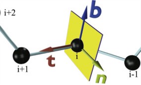
Figure 1: Color online: Definition of Frenet frames (1)-(3) at the position of a C$\alpha$ atom.

II.3 Pulchra, Remo and Scwrl4 frames

The framing used in Pulchra Rotkiewicz-2008 is obtained from four successive C$\alpha$ coordinates. We start by defining

$${\mathbf{e}}_{i,j}\ =\ \frac{\mathbf{r}_{i}-\mathbf{r}_{j}}{|\mathbf{r}_{i}-\mathbf{r}_{j}|}$$ (4)

The Pulchra frames ($\mathbf{\nu}_{x}^{i},\nu_{y}^{i},\nu_{z}^{i}$) are then

$${\mathbf{\nu}}^{i}_{x}\ =\ {\mathbf{e}}_{i-1,i+1}$$ (5)

$${\mathbf{\nu}}^{i}_{y}\ =\ \frac{\mathbf{e}_{i,i+1}\times\mathbf{e}_{i-1,i}}{|\mathbf{e}_{i,i+1}\times\mathbf{e}_{i-1,i}|}$$ (6)

$$\mathbf{\nu}^{i}_{z}=\mathbf{\nu}^{i}_{x}\times\mathbf{\nu}^{i}_{y}$$ (7)

The Remo Li-2009 reconstruction program uses also frames that are obtained from four successive C$\alpha$ coordinates: We again start with (4) and we set

The Remo frames are then

$${\mathbf{x}}_{i}\ =\ \frac{\mathbf{e}_{i-1,i+2}+\mathbf{e}_{i,i+1}}{|\mathbf{e}_{i-1,i+2}+\mathbf{e}_{i,i+1}|}$$ (8)

$$\mathbf{y}_{i}\ =\ \frac{\mathbf{e}_{i-1,i+2}-\mathbf{e}_{i,i+1}}{|\mathbf{e}_{i-1,i+2}-\mathbf{e}_{i,i+1}|}$$ (9)

$$\mathbf{z}_{i}\ =\ \mathbf{x}_{i}\times\mathbf{y}_{i}$$ (10)

Both Pulchra and Remo frames are very different from the discrete Frenet frames. In particular, both of these framings exploit four consecutive C$\alpha$ atoms, while the discrete Frenet frames use only three.

Finally, in the case of Scwrl4 the backbone is described in terms of the Ramachandran angles Krivov-2009 .

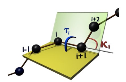
Figure 2: Color online: Definition of bond ($\kappa_{i}$) and torsion ($\tau_{i}$) angles in relation to the $i^{th}$ C$\alpha$ atom.

II.4 Visualization

For protein structure visualization and our data analysis, we use exclusively the Frenet frames ($\mathbf{n},\mathbf{b},\mathbf{t}$); for each C$\alpha$ atom we associate a (virtual) C$\alpha$ backbone bond ($\kappa$) and torsion ($\tau$) angle as follows,

$$\begin{matrix}\vspace{0.2cm}\kappa_{i}=\arccos(\mathbf{t}_{i+1}\cdot\mathbf{t}_{i})\\ \tau_{i}={\rm sign}(\mathbf{b}_{i+1}\cdot\mathbf{n}_{i})\arccos(\mathbf{b}_{i+1}\cdot\mathbf{b}_{i})\end{matrix}$$ (11)

These angles are shown in Figure 2. To visualize the various atoms in a protein, we identify the bond and torsion angles ($\kappa,\tau$) as the canonical latitude and longitude angles on the surface of a unit radius (Frenet) sphere $\mathbb{S}^{2}_{\alpha}$: The center of the sphere is located at the C$\alpha$ atom, the north-pole of $\mathbb{S}^{2}_{\alpha}$ is the point where the latitude angle $\kappa=0$, the vector $\mathbf{t}$ points to the direction of the north-pole and this direction coincides with the canonical $z$-direction in a C$\alpha$ centered Cartesian coordinate system. The great circle $\tau=0$ passes through the north-pole and the tip of the normal vector $\mathbf{n}$ that lies at the equator, the longitude a.k.a. torsion angle takes values $\tau\in[-\pi,\pi)$ and it increases in the counterclockwise direction around the positive $z$-axis i.e. around vector $\mathbf{t}$.

In the sequel, whenever we introduce a Frenet sphere $\mathbb{S}^{2}$ we shall use the convention that the triplet ($\mathbf{n},\mathbf{b},\mathbf{t}$) corresponds to the right-handed Cartesian ($xyz$)$\sim$($rgb$) coordinate system, with the convention that $\mathbf{n}\sim x\sim$ red ($r$), $\mathbf{b}\sim y\sim$ green ($g$) and $\mathbf{t}\sim z\sim$ blue ($b$). The color coding of distributions on the spheres are always relative but with equal MatLab setting, in all the cases that we display, and intensity increases from no-entry white to low density blue, and towards high density red.

We plot the directions of the peptide plane O and side chain C$\beta$ atoms on the surface of $\mathbb{S}^{2}_{\alpha}$ in exactly the way how they are seen from the position of a miniature observer, standing at the center of the sphere $\mathbb{S}^{2}_{\alpha}$ and with head up towards the north-pole. For the O atoms we use spherical coordinates that we denote ($\theta,\phi$) for the latitude and longitude, for the C$\beta$ atoms we denote the spherical coordinates ($\vartheta,\varphi$) for the latitude and longitude on $\mathbb{S}^{2}_{\alpha}$. Both sets of coordinates are in direct correspondence with ($\kappa,\tau$).

In Figure 3 we visualize the statistical reference distributions of the O and C$\beta$ atoms, in crystallographic Protein Data Bank structures that have been measured with better than 1.0 Å  resolution. We choose these, since we trust that such ultra high resolution structures are relatively void of refinement.

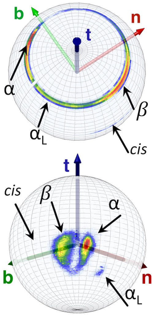
Figure 3: Color online: Top: The ($\theta,\phi$) distribution of peptide plane O atoms in the below 1.0 Å  resolution PDB structures on the surface of the Frenet sphere $\mathbb{S}^{2}_{\alpha}$. Bottom: The ($\vartheta,\varphi$) distribution of C$\beta$ atoms in the below 1.0 Å  resolution PDB structures on $\mathbb{S}^{2}_{\alpha}$. In both Fgures we have identified the major regions $\alpha$-helices ($\alpha$), $\beta$-strands ($\beta$), left-handed $\alpha$-helices ($\alpha_{L}$) and cis-peptide planes ($cis$).

The O distribution is concentrated on a very narrow circle-like annulus. It forms the base of a right circular cone with axis that coincides with the $\mathbf{t}$ vector and with conical apex at the center of the Frenet sphere; the latitude of the annulus is very close to $\theta=\pi/4$ (rad) so that the apex of the cone is very close to $\pi/2$. The regions of $\alpha$-helical and $\beta$-stranded regular structures are connected by a region of left-handed $\alpha$-helical structures and by a region of loops. There are very few entries outside this circular region; notably the cis-peptide plane region is located on a short strip under the $\beta$-stranded region with a latitude angle close to $\theta\approx\pi/2$.

The C$\beta$ distribution shown in Figure 3 is a little like a horse-shoe, forming a slightly distorted annulus that is somewhat wider than in the case of the O distribution. The regions of $\alpha$-helical and $\beta$-stranded regular structures are connected by a region of loops but the distribution of left-handed $\alpha$-helical structures is now disjoint from the main distribution.

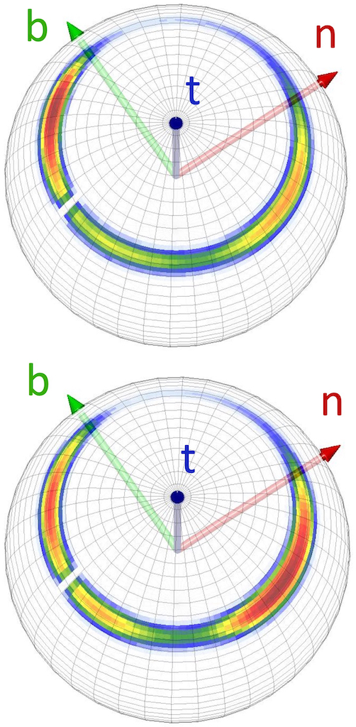
Figure 4: Color online: Top: The distribution of peptide plane O atoms in the villin trajectory of Anton. Bottom: The distribution of peptide plane O atoms in the ww-domain trajectory of Anton.

In Figures 4 and 5 we show the corresponding Anton distributions for the O an C$\beta$ atoms, separately in the case of villin and ww-domain. When we compare the Anton distributions and the ultra high resolution PDB data of Figure 3, we observe that the overall structure of the statistical distributions are very similar. We also note that as expected, in the villin trajectory there is a clear predominance of the $\alpha$-helical region, while in the case of ww-domain the $\beta$-stranded region dominates. The PDB and Anton distributions are otherwise remarkably similar, superficially the only difference appears to be due to thermal fluctuations in the latter: The crystallographic data is often taken at liquid nitrogen temperatures below 77 K while the simulation temperature in the Anton data is around 360K for both villin and ww-domain.

The strong similarity between the distributions in Figures 3-5 motivates us to make the following bold proposal: Even in the case of a dynamical protein under near-physiological conditions, the relative positions of the O and C$\beta$ atoms can be reconstructed with high accuracy from the knowledge of the C$\alpha$ atoms motion - at least when the CHARMM22^⋆ force field is used to describe the dynamics.

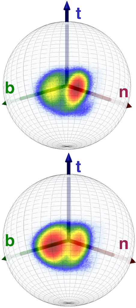
Figure 5: Color online: Top: The distribution of side chain C$\beta$ atoms in the villin trajectory of Anton. Bottom: The distribution of side chain C$\beta$ atoms in the ww-domain trajectory of Anton.

II.5 Reconstruction

We proceed to try and reproduce the individual O and C$\beta$ atom positions in the Anton trajectories of villin and ww-domain Lindorff-2011 , solely from the knowledge of the C$\alpha$ atoms. We employ four different reconstruction methods:

II.5.1 Pulchra

For Pulchra Rotkiewicz-2008 we use the version 3.04. We start with the C$\alpha$ coordinates that we obtain from Anton. We then use Pulchra to reconstruct the other heavy atom positions, with only the instantaneous C$\alpha$ coordinates of the Anton trajectory as an input. From the Pulchra structures we read the coordinates of the peptide plane O and side chain C$\beta$ atoms, and compare with the original Anton data.

II.5.2 Remo

For Remo Li-2009 we use the version 3.0, and we proceed with reconstruction as in the case of Pulchra. We note that Remo employs Scwrl for the side chains.

II.5.3 Scwrl4

For stand-alone Scwrl Krivov-2009 we use the version 4.0. Since Scwrl can not reconstruct the peptide planes, we use it only for the C$\beta$ comparison. For this we first construct the peptide planes using Pulchra, since Remo is already based on Scwrl.

II.5.4 Statistical Method

Unlike the previous three methods, our Statistical Method approach to reconstruction does not employ any force field refinement, stereochemical constraints, or any other kind of data curation. It only uses statistical analysis of PDB data to predict the positions of the peptide plane O and side chain C$\beta$ atoms from the knowledge of the C$\alpha$ atom positions: Once the C$\alpha$ coordinates of an amino acid are given, a search algorithm fits it with a PDB structure and identifies the ensuing O and C$\beta$ atom coordinates as the reconstructed coordinates.

As already stated, the PDB pool consist of all those crystallographic structures that have been measured with better than 1.0 Å  resolution. We start with a visual presentation of the C$\alpha$ bond and torsion angle density distribution of these PDB structures, in terms of a stereographically projected Frenet sphere.

Let $\mathbb{S}^{2}_{\alpha}(i)$ be centered at the $i^{th}$ C$\alpha$ atom of a given PDB structure. The vector $\mathbf{t}_{i}$ has its tail at the center of $\mathbb{S}^{2}_{\alpha}(i)$ and its head lies at the north pole, this vector points from the $i^{th}$ C$\alpha$ atom towards the $(i+1)^{st}$ C$\alpha$ atom. The $(i+2)^{nd}$ C$\alpha$ is then located similarly, in the direction of the Frenet vector $\mathbf{t}_{i+1}$ that points from the center of $\mathbb{S}^{2}_{\alpha}(i+1)$ towards its north pole.

We parallel transport the vector $\mathbf{t}_{i+1}$ without any rotation until its tail becomes located at the $i^{th}$ C$\alpha$ atom position i.e. at the origin of $\mathbb{S}^{2}_{\alpha}(i)$. Let ($\kappa_{i},\tau_{i}$) be the Frenet frame coordinates of the head of the parallel transported $\mathbf{t}_{i+1}$ on the surface of $\mathbb{S}^{2}_{\alpha}(i)$. These coordinates depict how a miniature Frenet frame observer, standing at the position of the $i^{th}$ C$\alpha$ atom and head towards the north pole of $\mathbb{S}^{2}_{\alpha}(i)$, sees the backbone twisting and bending when she proceeds along the chain to the position of the $(i+1)^{st}$ C$\alpha$ atom.

We repeat the construction for all the C$\alpha$ atoms along all the chains in our pool. This yields us a statistical distribution in terms of the coordinates ($\kappa,\tau$) of the heads of the parallel transported vectors $\mathbf{t}$. We visualize the distribution by projecting the sphere $\mathbb{S}^{2}_{\alpha}$ stereographically onto the complex plane from the south pole as shown in Figure 6.

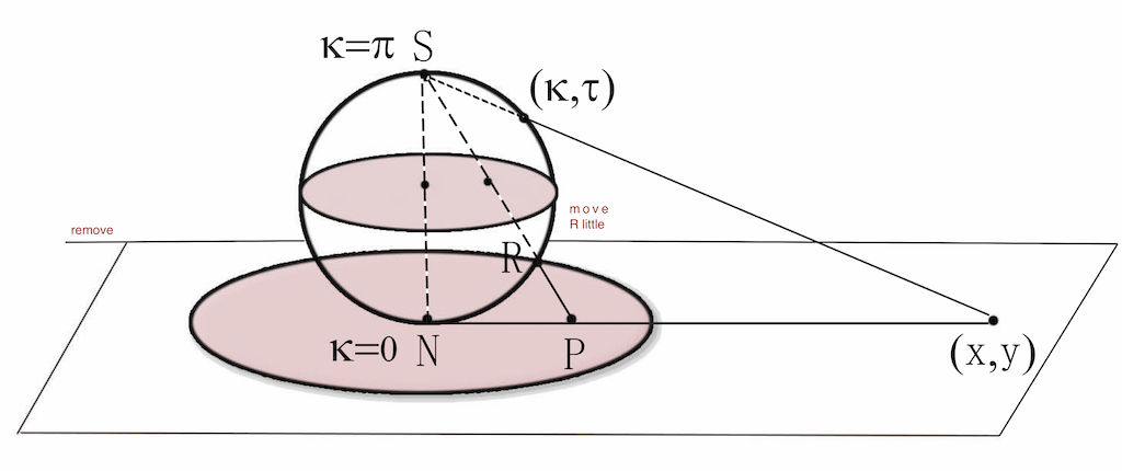
Figure 6: Color online: Stereographic projection of two sphere onto plane, with the projection taken from the south-pole.

The relation between the spherical coordinates ($\kappa,\tau$) and the $z=x+iy$ coordinates on the plane is

$$x+iy=\tan\left(\frac{\kappa}{2}\right)e^{i\tau}$$

In Figure 7 we show the distribution of all the C$\alpha$ atom coordinates in our PDB data set, on the stereographically projected Frenet sphere.

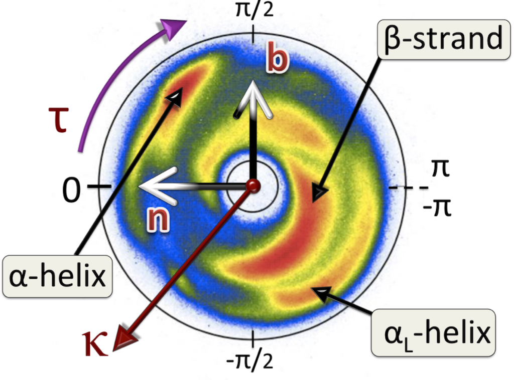
Figure 7: Color online: Statistical distribution of all C$\alpha$ atoms in our 1.0 Å  pool of PDB structures, on stereographically projected sphere shown in Figure 6.

The distribution is largely concentrated inside an annulus, with inner circle $\kappa_{in}\approx 1$ and outer circle $\kappa_{out}\approx\pi/2$. The various regular secondary structures such as $\alpha$-helices, $\beta$-strands and left-handed $\alpha$-helices are clearly identifiable and marked in this Figure.

We proceed to describe how we predict the positions of the O and C$\beta$ atoms from the knowledge of the C$\alpha$ atoms coordinates, along a given (dynamical) protein structure: We first use the torsion angle $\tau\in[-\pi,\pi)$ to divide the statistical distribution of Figure 7 into 60 equal size sectors sized $\Delta\tau=\pi/30$ radians. We then divide each of these sectors into two sets, one with bond angle $\kappa<1.2$ (rad) and the other with $\kappa\geq 1.2$ (rad); we choose this value since the circle $\kappa=1.2$ divides the annulus in Figure 7 roughly into annuli of $\alpha$-helix-like and $\beta$-strand-like (secondary) structures.

Now suppose that we have a C$\alpha$ atom along a protein backbone, with coordinates ($\kappa_{i},\tau_{i}$). We determine the coordinates ($\theta_{i},\phi_{i}$) of the corresponding O atom and the coordinates ($\vartheta_{i},\varphi_{i}$) of the corresponding C$\beta$ atom using the following algorithm:

Step 1:  We first use the $\tau_{i}$ value of the C$\alpha$ atom to select the pertinent sector $\tau_{i}\in\Delta\tau$. We then use its $\kappa_{i}$ value together with $\kappa_{i+1}$ of the following C$\alpha$ atom along the chain, to assign with the given C$\alpha$ atom one of the four sets

$$\begin{matrix}{\rm Set~{}\Delta\kappa_{1}:}~{}~{}~{}~{}~{}~{}~{}~{}\kappa_{i}\ <\ 1.2\ \ \ \ \&\ \ \ \ \kappa_{i+1}\ <\ 1.2\\ {\rm Set~{}\Delta\kappa_{2}:}~{}~{}~{}~{}~{}~{}~{}~{}\kappa_{i}\ <\ 1.2\ \ \ \ \&\ \ \ \ \kappa_{i+1}\ \geq\ 1.2\\ {\rm Set~{}\Delta\kappa_{3}:}~{}~{}~{}~{}~{}~{}~{}~{}\kappa_{i}\ \geq\ 1.2\ \ \ \ \&\ \ \ \ \kappa_{i+1}\ <\ 1.2\\ {\rm Set~{}\Delta\kappa_{4}:}~{}~{}~{}~{}~{}~{}~{}~{}\kappa_{i}\ \geq\ 1.2\ \ \ \ \&\ \ \ \ \kappa_{i+1}\ \geq\ 1.2\end{matrix}$$

Together with the $\Delta\tau$ sectors this divides our statistical C$\alpha$ distribution into 4$\times$60 subsets $[\Delta\kappa;\Delta\tau]$, and we choose the one that corresponds to the ($\kappa_{i},\kappa_{i+1},\tau_{i}$) values of the C$\alpha$ atom we consider.

Step 2:  We search a protein structure in our pool, in the subset $[\Delta\kappa,\Delta\tau]$ of the $i^{th}$ C$\alpha$, for which two consecutive amino acids are also identical to the $i^{th}$ and $(i+1)^{st}$ amino acids of the protein structure that we consider.

$\bullet~{}$ If we find only one matching pair of amino acids in the subset $[\Delta\kappa,\Delta\tau]$, we use the coordinates of its O and C$\beta$ atoms as the predicted coordinates of the O, C$\beta$ atoms of the $i^{th}$ C$\alpha$ atom.

$\bullet~{}$ If there are two or more matching pairs, we use the average value of their O and C$\beta$ coordinates to determine those of the O and C$\beta$ around the C$\alpha$ of interest.

$\bullet~{}$ If there are no pairs of identical amino acids in the subset $[\Delta\kappa,\Delta\tau]$, we use the average value of all PDB structures in this subset to determine the O and C$\beta$ coordinates.

$\bullet~{}$ Finally, if the subset $[\Delta\kappa,\Delta\tau]$ is empty we search for one from a neighboring subset, first from preceding $\Delta\tau$, then from following $\Delta\tau$, then from neighboring $\Delta\kappa$; but such cases are highly exceptional.

Step 3:  We repeat the process for all C$\alpha$ atoms along the chain. At the end of the chain there is no $\kappa_{i+1}$, thus at the end of the chain we use only the $\kappa_{i}$ value in our search.

Our reconstruction algorithm is extremely simple and proceeds very fast computationally, much faster than any of the other three reconstruction programs we consider, even though we have not optimized the search algorithm but use a straightforward MatLab code.

The sector size $\Delta\tau$ can be changed and optimised; here we have chosen 60 sectors, only to exemplify the method.

The reason why we divide the original annulus into two using $\kappa=1.2$ in our search algorithm is, that while a torsion angle is determined by four C$\alpha$ atoms, in the case of a bond angle only three C$\alpha$ are needed; see Figure 2. Thus, by engaging the two neighboring bond angle values, we employ the full information in all four C$\alpha$ atoms in our search algorithm.

In Step 2, we calculate the average values of the angles as follows: For the average latitude $\theta_{ave}$ (similarly for $\vartheta_{ave}$) we simply use

$$\theta_{ave}\ =\ \frac{1}{N}\sum\limits_{i=k}^{N}\theta_{k}$$

where the summation is over all elements in the given subset $[\Delta\kappa,\Delta\tau]$. For the average longitude $\phi_{ave}$ (similarly for $\varphi_{ave}$) we proceed as follows: We first define

$$X\ =\ \frac{1}{N}\sum\limits_{i=k}^{N}\cos\phi_{k}\ \ \ \ \ \&\ \ \ \ \ Y\ =\ \frac{1}{N}\sum\limits_{i=k}^{N}\sin\phi_{k}$$

and

$$R=\sqrt{X^{2}+Y^{2}}$$

The average value is then obtained from

$$\cos\phi_{ave}\ =\ \frac{X}{R}\ \ \ \ \ \&\ \ \ \ \ \sin\phi_{ave}\ =\ \frac{Y}{R}$$

II.6 Algorithm comparisons

II.6.1 Direction comparison

In order to compare the different reconstruction methods we introduce two unit length vectors $\overrightarrow{C\alpha O}$ and $\overrightarrow{C\alpha\beta}$; the former points from the C$\alpha$ atom to the following peptide plane O atom ($X=$  O in the sequel), and the latter points from the C$\alpha$ atom to its side chain C$\beta$ atom ($X=\beta$ in the sequel). We evaluate these vectors for all residues $i=1,...,N$ and for every structure $k=1,...,K$ in the Anton data. We also evaluate these vectors in all of the four reconstruction methods and in the sequel $\rm y=\rm P,R,S,M$ stands for Pulchra (P), Remo (R), Scwrl4 (S) and the Statistical Method (M) respectively.

We define $\Theta^{\rm y}_{\rm X}[i,k]$ to be the angle between a vector $\overrightarrow{C\alpha X}$ evaluated from the Anton data, and the corresponding vector obtained from the corresponding reconstruction method. The statistical distribution function for all the values $\Theta^{\rm y}_{\rm X}[i,k]$ measures the overall accuracy of a given method, for reconstructing the individual O and C$\beta$ atom positions.

For each of the $k=1,...,K$ Anton chain structure, we evaluate the root-mean-square (RMS) value of the angles $\Theta^{\rm y}_{\rm X}[i,k]$ by summing over the $N$ individual residues of the chain,

$${\rm RMS}\,[\Theta^{\rm y}_{\rm X}(k)]\ =\ \sqrt{\frac{1}{N}\sum\limits_{i=1}^{N}\left(\Theta^{\rm y}_{\rm X}[i,k]\right)^{2}}$$ (12)

The distribution density (12) then measures the overall accuracy of a method, in the reconstruction of the C$\alpha$-O-C$\beta$ chains.

II.6.2 Distance comparison

We also compare the algorithms by evaluating the RMS distance between different atomic positions in the Anton trajectory and in the reconstructed trajectory. The RMS distance between two chain structures is evaluated from

$${\rm RMSD}(X;k)=\sqrt{\frac{1}{N}\sum\limits_{i=1}^{N}|\mathbf{r}_{i,X}^{A,k}-\mathbf{r}_{i,X}^{y,k}|^{2}}$$ (13)

Here $\mathbf{r}_{i,X}^{A,k}$ is the Anton data distance between the C$\alpha$ atom and the $X={\rm O},\,\beta$ atom at residue $i$ in structure $k$, and $\mathbf{r}_{i,X}^{y,k}$ is the corresponding quantity in the $y=\rm P,R,S,M$ reconstructed structure. The probability distribution of (13) is a complement of (12), as a measure of the overall accuracy of a method in the reconstruction of the entire chain in a statistical sense.

For reference, in Figure 8 we present the combined distribution of the Debye-Waller fluctuation distances

$$\sqrt{<|\mathbf{x}|^{2}>}\ =\ \sqrt{\frac{B}{8\pi^{2}}}$$

for the O and C$\beta$ atoms, that we have evaluated using the $B$-factors in our 1.0 Å  PDB pool; note the logarithmic scale. The fluctuation distances are strongly peaked at around 0.3 Å, and there are practically no structures with a fluctuation distance less than 0.12 Å.

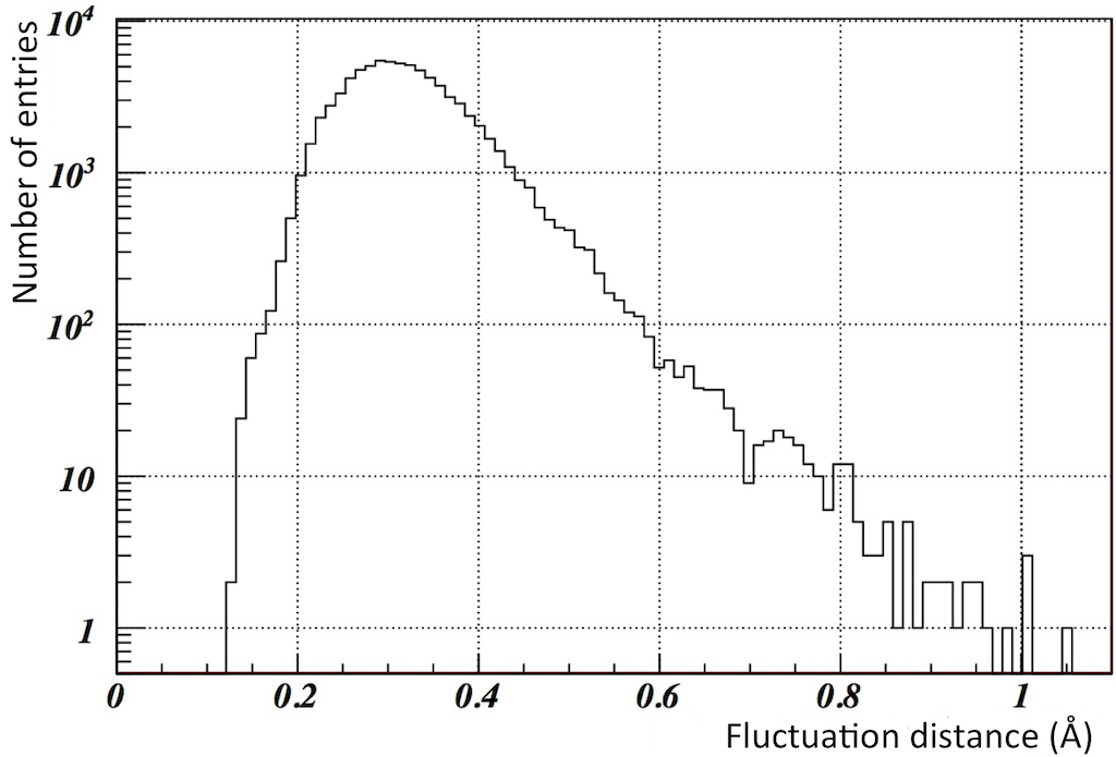
Figure 8: Color online: Combined B-factor fluctuation distances for the O and C$\beta$ atoms

Similarly, Figure 9 shows the statistical distributions in the individual C$\alpha$-O and C$\alpha$-C$\beta$ distances that we calculate directly from the coordinates in our PDB data pool and Anton data, respectively; only results for villin are shown as the results for ww-domain are very similar.

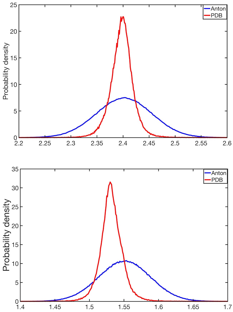
Figure 9: Color online: distribution of distances in Ångström, calculated directly from the coordinates in our PDB data and Anton data for villin. Top: C$\alpha$-O Bottom: C$\alpha$-C$\beta$.

In the following we shall not refine the C$\alpha$-O and the C$\alpha$-C$\beta$ distances, in our statistical method, the differences are in any case minor. Instead we simply use the average PDB distance values

$$\begin{matrix}\Delta r\ =\ 2.40\ {\rm\AA}\ \ \ \ \ \ \ {\rm For~{}C\alpha-O~{}distance}\\ \hskip 4.26773pt\Delta r\ =\ 1.53\ {\rm\AA}\ \ \ \ \ \ \ {\rm For~{}C\alpha-C\beta~{}distance}\\ \end{matrix}$$

in our Statistical Method reconstruction. It is natural to allocate the larger variance in the case of Anton data in Figures 9 to temperature fluctuations.

III Results

III.1 Peptide plane O atoms

We start with the peptide plane O atom distributions in the Anton data. We compare the Anton results shown in Figure 4, with results from Pulchra , Remo and Statistical Method.

III.1.1 Frenet Spheres

In Figures 10 we present the reconstructed O atom distributions on a Frenet sphere $\mathbb{S}^{2}$, in the case of villin. The Figures display all the reconstructed O atom coordinates ($\theta,\phi$) for all the C$\alpha$ atoms of all Anton trajectories that we obtain using Pulchra, Remo and Statistical Method respectively.

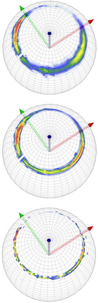
Figure 10: Color online: Top: Reconstructed peptide plane O distribution for villin on Frenet sphere $\mathbb{S}^{2}$. Top: Pulchra Middle: Remo Bottom: Statistical Method.

Overall, all three distributions reproduce well the O atom villin distribution of the Anton trajectory in Figure 4 (top). In particular, the regular $\alpha$-helical and $\beta$-stranded regions are clearly identifiable. We observe that both Pulchra and Remo distributions are slightly wider than the PDB distribution, we propose that this reflects mainly the presence of thermal effects in the Anton data, as captured by these two methods. On the other hand, the Statistical Method distribution is more concentrated. This is expected since the data pool is a subset of the PDB data shown in Figure 4 (top), which have all been measured at very low temperature values.

We remind that the color coding is always relative but equal, in all the cases that we display, and intensity increases from no-entry white to low density blue, and towards high density red.

In Figures 11 we present the reconstructed O distributions in the case of ww-domain. Again, all three distributions are very much in line with the Anton data of Figure 4 (bottom). We observe some fragmentation and excess (thermal) data spreading in the case of Pulchra. The Remo distribution also displays thermal spreading while the Statistical Method distribution is again more concentrated, as expected since it forms a subset of the low temperature PDB data.

We now analyze the reconstruction results for the peptide plane O atoms in more detail, using the methods of Section II F.

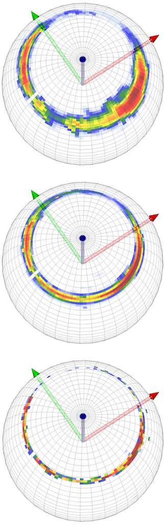
Figure 11: Color online: Top: Reconstruction of peptide plane O distribution on the sphere $\mathbb{S}_{\alpha}^{2}$ for ww-domain. Top: Pulchra Middle: Remo Bottom: Statistical Method.

III.1.2 Individual angular probability densities for peptide planes

In Figures 12 and 13 we show the normalized probability density distributions for all the individual angles $\Theta^{\rm y}_{\rm O}[i,k]$ along the Anton trajectories for Pulchra, Remo and the Statistical method in the case of villin and ww-domain O atoms, respectively.

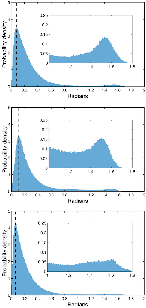
Figure 12: Color online: Probability density distribution for all individual angles $\Theta^{\rm y}_{\rm O}[i,k]$ in the case of Anton villin trajectories. Top: Pulchra Middle: Remo Bottom: Statistical Method.

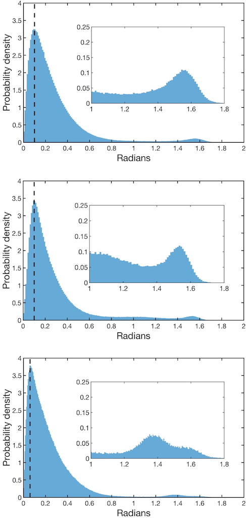
Figure 13: Color online: Probability density distribution for all angles $\Theta^{\rm y}_{\rm O}[i,k]$ along the Anton ww-domain trajectories. Top: Pulchra Middle: Remo Bottom: Statistical Method.

In both Pulchra and Remo the individual $\Theta^{\rm y}_{\rm O}[i,k]$ values peak near the small value $\Theta_{max}\approx 0.1$ (rad). For the Statistical Method the peak is located at the even smaller value $\Theta_{max}\approx 0.06$ (rad), both in the case of villin and ww-domain.

From Figure 9 we learn that the average PDB distance between C$\alpha$ and O is around 2.4 Å. An angular deviation of $\Theta_{max}\approx 0.06$ then corresponds to a distance deviation $\sim 0.14$ Å  which is smaller than the B-factor fluctuation distances in Figure 8 and more in line with the (apparently purely thermal) distance deviations we observe in Figures 9.

We conclude that each of the three methods can reconstruct the individual angular positions of the dynamical Anton O atoms with very high precision. Moreover, despite its simplicity the Statistical Method performs even better than both Pulchra and Remo.

In each of the probability distributions of Figures 12, 13 we observe enhanced accumulation of data near $\Theta\approx\pi/2$; the inserts show the probability densities for $\Theta$-values above 1.0 (rad). We recall our interpretation of the Frenet sphere O distribution as the base of a cone, with the apex at the origin; the vertex angle has a value very close to $\pi/2$. Thus the $\Theta\approx\pi/2$ secondary peak corresponds to a $\phi\sim$180 degree rotation around the (blue) $\mathbf{t}$-vector in the Figures 10, 11. We observe that a rotation of the longitude $\phi$ by $\sim 180^{\rm o}$ exchanges the $\alpha$-helical and $\beta$-stranded regions according to top Figure 3.

III.1.3 Angular probability densities for entire chains

In Figures 14, 15 we show the probability density distributions (12) for Pulchra, Remo and Statistical Method, in the case of villin and ww-domain O atoms, respectively. We remind that the value of (12) is a measure for the accuracy of the reconstruction, in the case of the entire chain.

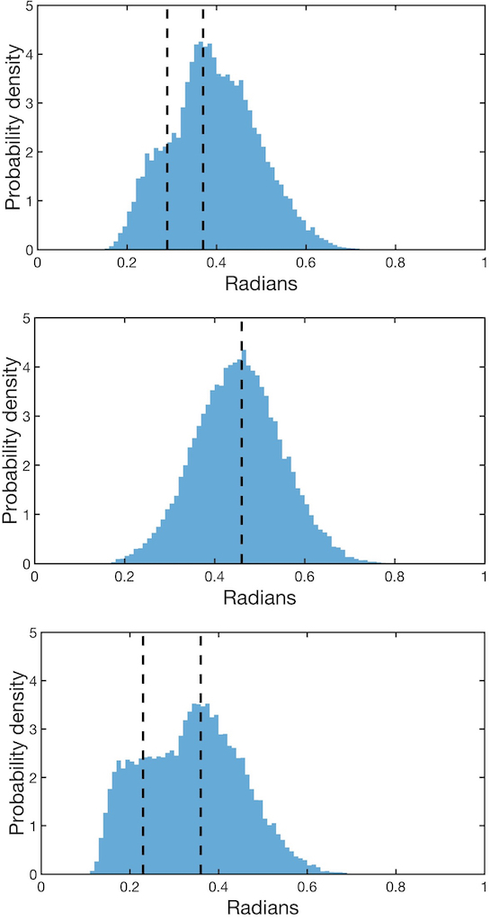
Figure 14: Color online: The probability density distributions (12) for villin. Top: Pulchra Middle: Remo Bottom: Statistical Method.

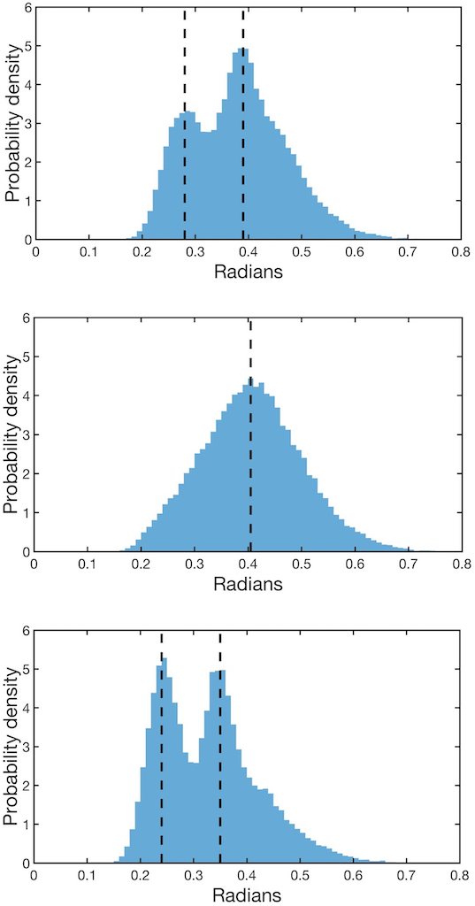
Figure 15: Color online: The probability density distributions (12) for ww-domain. Top: Pulchra Middle: Remo Bottom: Statistical Method.

In each case, the reconstructed chains appear to be very close to the original Anton chains, both in the case of villin and ww-domain. The Statistical Method performs best and the results for Pulchra are quite similar, but for Remo we observe a clear deviation from the Statistical method; the results from the latter are visibly better.

Note that in the case of both Pulchra and Statistical Method, both the villin and the ww-domain profiles appear to resemble a combination of two distinct Gaussian distributions. On the other hand, in the case of Remo the distribution is like a single Gaussian (thermal spread), in both cases.

III.1.4 RMSD probability densities for entire chains

In Figures 16, 17 we show the probability density distributions for the RMS distances (13), evaluated for the entire C$\alpha$-O reconstructed chains that we obtain using Pulchra, Remo and Statistical Method in the case of villin and ww-domain Anton trajectories.

Figure 16: Color online: The probability density distributions for the RMS distance (13) over the O atoms in the case of villin. Top: Pulchra Middle: Remo Bottom: Statistical Method.

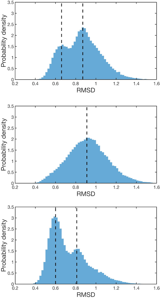
Figure 17: Color online: The probability density distributions for the RMS distance (13) over the O atoms in the case of ww-domain. Top: Pulchra Middle: Remo Bottom: Statistical Method.

Again, the reconstruction by the Statistical Method is closest to the original Anton result. The difference to Pulchra is very small but there is a more visible difference to Remo.

Even though all the RMS distances between the O-chains shown in Figures 16 and 17 are small, they are slightly larger than what we can expect on the basis of the individual (O and C$\beta$) atom B-factor fluctuation distances in Figure 8. In line with Figures 14, 15, both Pulchra and Statistical Method distributions again exhibit a double Gaussian profile; In the case of Remo the distributions form a single Gaussian which is more in line with a thermal spread, except that the peak is close to 1.0 Å  which is a somewhat large value in comparison to the Statistical Method where the two peaks are slightly below values 0.6 Å  and 0.8 Å  i.e. close to the covalent radius $\sim 0.66$ Å  of O atom. But even in the case of Remo, the deviation distances can be considered to be quite small and we consider the results to be good.

III.1.5 Peptide plane flip

In Figures 12 and 13 we have noted an accumulation of entries near $\Theta\sim\pi/2$, corresponding to a $\sim$180 degree rotation of the entire probability distribution around the $\mathbf{t}$ vector. Consequently these entries contribute maximally to the deviations between the Anton chain and the reconstructed chains, in terms of statistical distributions. We note that $\Theta\sim\pi/2$ corresponds to $\sim 3.4$ Å  in terms of spatial distance.

We consider only those Anton entries for which $\Theta>1.0$ simultaneously, in all of the three reconstruction methods; the spatial distance for two entries that are $\Theta\sim 1.0$ apart is $\sim$2.3 Å  which is way above the range of B-factor fluctuations in Figure 8. Thus, the $\Theta>1.0$ entries that are common to all three methods should be very little prone to method dependent fallacies, these entries should correspond to definite deviations in Anton data from PDB structures. There are a total of around 6.000 such entries, this corresponds to a mere 0.6 per cent of the total entries that we have analyzed. We evaluate the average values of $\Theta$ for all these entries. The probability distribution for these average values is concentrated very close to $\Theta=\pi/2$ as shown in Figure 18 (top). The entries are also distributed quite evenly around the O-circle on the Frenet sphere (Figure 18) (bottom), they seem to appear quite randomly during the Anton time evolution, and correspond to very sudden and short-lived 180 degree back-and-forth rotations (flips) of the entire peptide plane, around the virtual bond that connect two consecutive C$\alpha$ atoms.

From the available Anton data, we are unable to conclude whether these peptide plane flips are genuine physical effects with an important role in protein folding, or whether they are mere simulation artifacts, or whether they are effects that are specific to the CHARMM22^⋆ force field Piana-2011 . For example, it appears that in the Anton simulations the peptide plane N-H covalent bond lengths are constrained to have a fixed value. That may affect the stability of peptide planes, causing them to flip by 180 degrees.

To properly understand the character of these peptide plane flips one needs to perform more detailed all atom simulations, presumably with shorter time steps than used in Anton simulations and with no length constraints on the N-H covalent bonds.

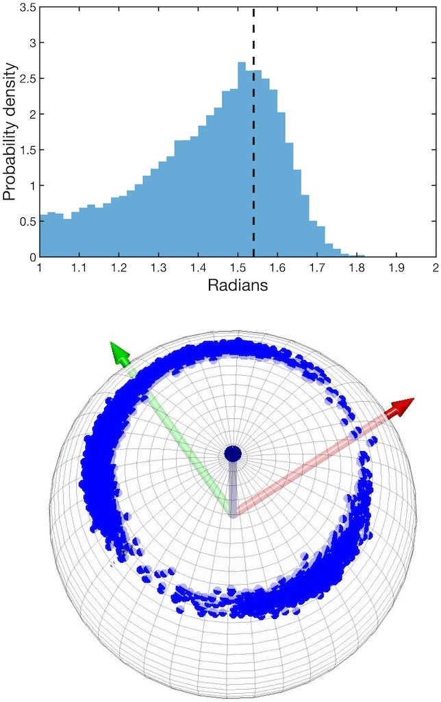
Figure 18: Color online: Top: The distribution of average value of angular deviations for the reconstructed entries with $\Theta>1.0$ (rad) in Figures 12 (villin). Bottom: The distribution of these entries on the Frenet sphere (ww-domain).

III.1.6 Double Gaussians

In Figures 14-17 we have observed the presence of a double Gaussian peak structures, in the Pulchra and Statistical Method distributions. We now proceed to try and identify the cause. We present a detailed analysis of the double Gaussian structures in the case of the Statistical Method RMSD distributions in Figures 16 and 17; the analysis in the other cases is similar, with similar conclusions.

In Lindorff-2011 the following quantity

$$Q(t)\ =\ \frac{\sum_{i=1}^{N_{res}}\sum_{j=1}^{N_{i}}\ \left[1+e^{10(d_{ij}(t)-(d^{0}_{ij}+1))}\right]^{-1}}{\sum_{i=1}^{N_{res}}N_{i}}$$ (14)

has been introduced, to characterize the distance of a dynamical chain at time $t$, to an experimentally measured folded state. Here $N_{i}$ is the number of contacts of residue $i$ along the chain as defined in Lindorff-2011 , $d_{ij}(t)$ is the distance in Å  between the C$\alpha$ atoms of residues $i$ and $j$ at time $t$ and $d_{ij}^{0}$ is the same distance in the natively folded, crystallographic structure. According to Lindorff-2011 a structure with $Q>0.9$ is folded and a structure with $Q<0.1$ is unfolded.

Consider now the two Statistical Method peaks in the villin distribution Figure 16 and in the ww-domain distribution Figure 17. In both cases, we analyze separately the low RMSD subsets with values below 0.54 Å  in villin and below 0.6 Å  in ww-domain, and the high RMSD subsets with RMSD values above 0.77 Å  in villin and above 0.8 Å  in ww-domain. These four subsets are identified by the dashed lines in the Figures. In Figures 19 we show the probability density distributions for the values of (14) that we evaluate for these subsets. Both in the case of villin and ww-domain the low-RMSD peak corresponds to large values of $Q$ which is characteristic to near-folded state, while the large-RMSD peak corresponds to predominantly small values of $Q$ which are characteristic to unfolded states.

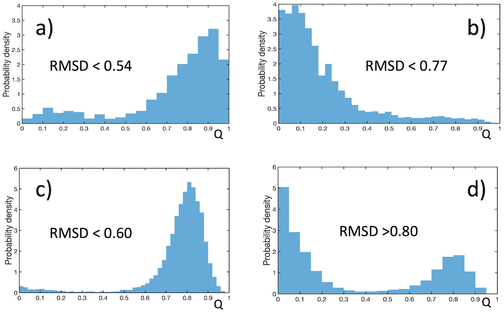
Figure 19: Color online: Statistical Method probability distributions for the $Q$-values (14), corresponding to the Gaussian peaks in Figures 16 and 17 a) low-RMSD villin, b) high-RMSD villin, c) low-RMSD ww-domain, d) high-RMSD ww-domain.

III.2 Side chain C$\beta$ atoms

We proceed to describe results from the C$\beta$ atom reconstruction. Due to the high accuracy in all the methods we use, the presentation is less detailed than in the case of peptide plane O atoms: The differences to Anton simulation results are minuscule.

We investigate reconstruction results in four approaches: Pulchra, Remo, Pulchra+Scwrl4, and our Statistical method. We note that Remo commonly constructs the side chain atoms using Scwrl while Pulchra employs its own side chain reconstruction. Thus we have added a Pulchra+Scwrl4 combination, where the peptide planes are first constructed with Pulchra and then side chains are constructed with Scwrl4. This combination should be of interest, since we have found that Pulchra performs slightly better than Remo in the reconstruction of the Anton peptide plane O atom positions.

III.2.1 Frenet spheres

In Figures 20 and 21 we have the Frenet sphere probability distributions for the four methods, in the case of villin and ww-domain respectively.

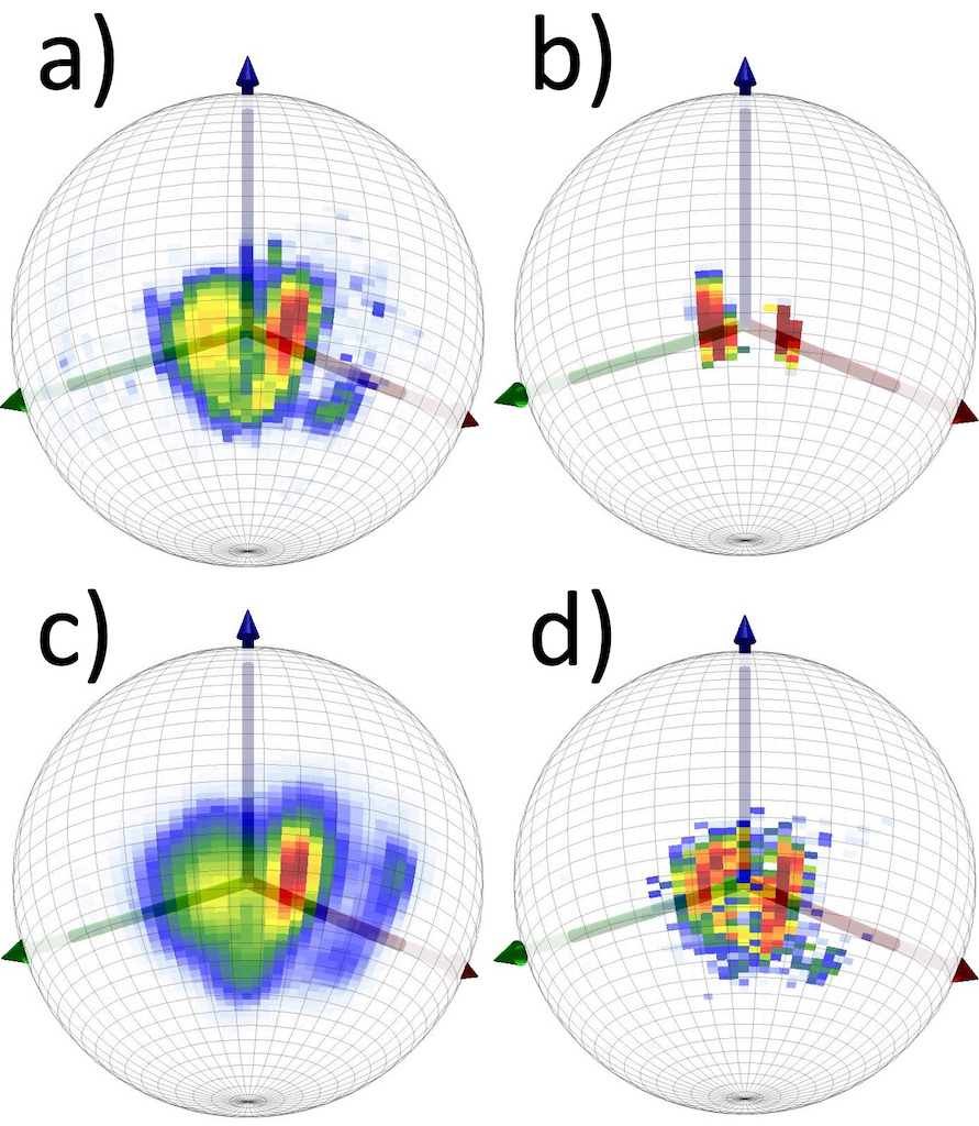
Figure 20: Color online: Reconstructed side chain C$\beta$ distribution for villin on the Frenet sphere $\mathbb{S}^{2}_{\alpha}$. Figure a) Pulchra, Figure b) Remo, Figure c) Pulchra+Scwrl4, Figure d) Statistical Method

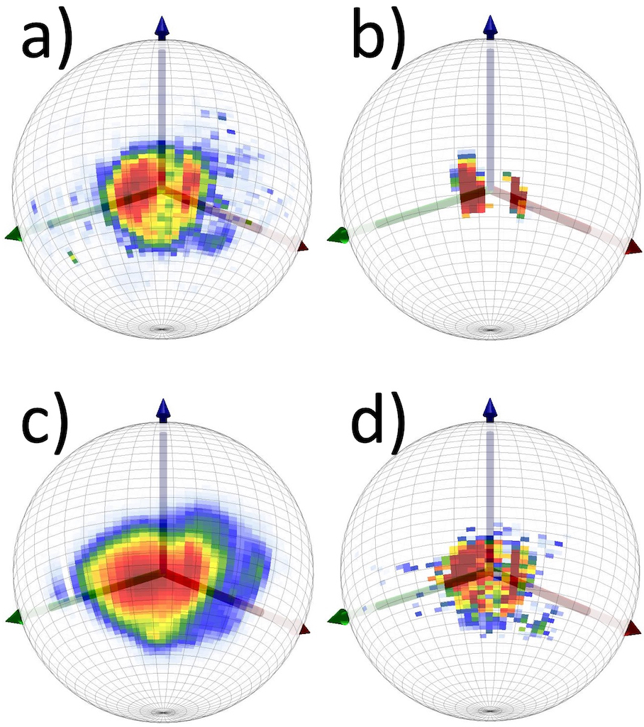
Figure 21: Color online: Reconstructed side chain C$\beta$ distribution for ww-domain on the Frenet sphere $\mathbb{S}^{2}_{\alpha}$. Figure a) Pulchra, Figure b) Remo, Figure c) Pulchra+Scwrl4, Figure d) Statistical Method

Pulchra reconstructs quite accurately the Anton distributions of the C$\beta$ atoms, shown in Figure 5. In particular, it reconstructs the region of left-handed $\alpha$-helices. Pulchra also broadens the overall shape of the distribution in a manner which, at least superficially, appears to account for the thermal fluctuations that are present in the Anton distributions.

Pulchra and Scwrlt4 combination increases the spread of the C$\beta$ distributions, there is now an even better resemblance between the Anton distributions with the (perceived) thermal fluctuations.

Remo reconstruct the C$\beta$ distributions in terms of very concentrated distributions that are highly peaked at the C$\alpha$ and C$\beta$ regions, with no observable thermal spreading: Remo appears to reconstruct the C$\beta$ positions in a very straightforward two-stage fashion. In particular, there is a marked difference between the Pulchra+Scwrl4 and Remo distributions even though Remo apparently uses Scwrl for side chain reconstruction Li-2009 .

Statistical Method selects a subset of the full PDB distribution in Figure 3 (bottom), as expected. Since the PDB data has been mostly measured at liquid nitrogen temperatures below $\sim$77 K, the distributions do not display thermal spreading.

III.2.2 Individual angular probability densities for side chains

In Figure 22 we have combined the probability distribution functions for the individual angles $\Theta^{\rm y}_{\beta}[i,k]$ in the case of C$\beta$, for all the four reconstruction methods we consider. We observe very little difference between the four methods, all distributions are strongly peaked near $\Theta\approx 0.15$ (rad). According to Figure 9 (bottom) the PDB average for the C$\alpha$-C$\beta$ bond length is around 1.54 Å. Thus a $\Theta\approx 0.15$ (rad) angular deviation corresponds to an average distance deviation of around 0.2 Å  which is well within the the limits of the individual B-factor fluctuation distances in Figure 8.

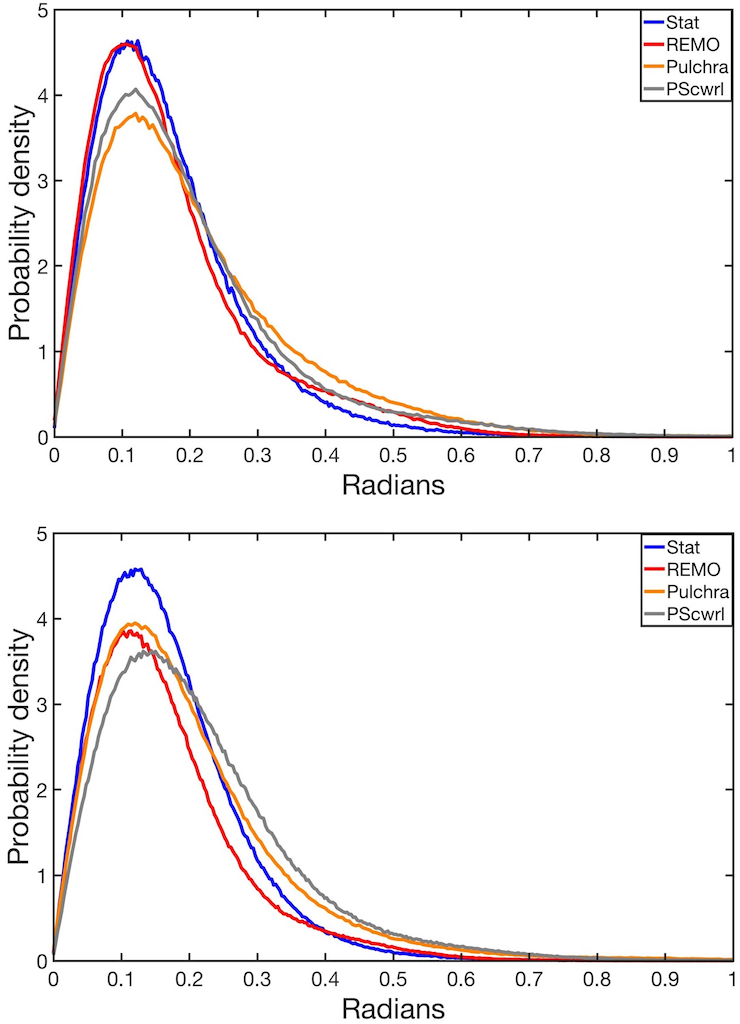
Figure 22: Color online: Probability distribution for the individual angular deviations $\Theta^{y}_{\beta}[i;k]$ in the four reconstruction methods.Top: villin and Bottom: ww-domain.

III.2.3 RMS Probability densities for reconstructed chains

Figures 23 show the C$\beta$ probability distributions of (12) and Figures 24 show the C$\beta$ probability distributions of (13), for the reconstructed chains. Generally speaking, all four methods are able to reconstruct the C$\beta$ positions with high accuracy. The Statistical Method performs best but the difference to Remo is tiny. For Pulchra the results are slightly worse: Its combination with Scwrl4 performs a bit better than Pulchra alone in the case of villin, but in the case of ww-domain the results are opposite. However, the differences between all the four methods are quite small, and the RMS distances are all in line with the experimental B-factor fluctuation distances shown in Figure 8.

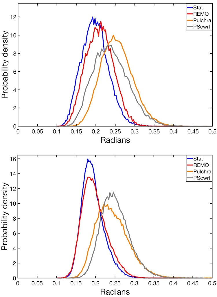
Figure 23: Color online: Probability distribution for the angular RMS values (12) in the four reconstruction methods. Top: villin and Bottom: ww-domain.

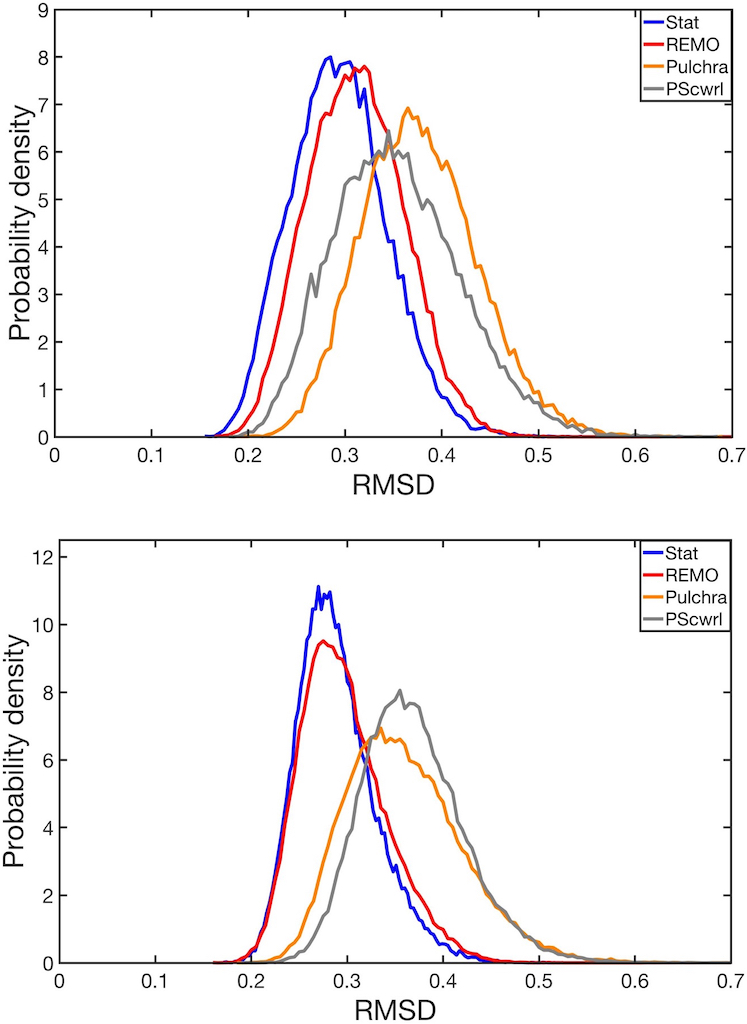
Figure 24: Color online: Probability distribution for the RMS distances (13) in the four reconstruction methods. Top: villin and Bottom: ww-domain.

IV Conclusions

To comprehend protein dynamics is a prerequisite for the ability to understand how biologically active proteins function. However, despite the importance of protein dynamics, our knowledge remains very limited. High quality experimental data on dynamical proteins at near-physiological conditions is sparse and very difficult to come by, the primary source of information is theoretical considerations in combination with all atom molecular dynamics simulations; the latter are best exemplified by the very long Anton trajectories Lindorff-2011

Here we have searched for systematics in the dynamics of proteins at near-physiological conditions, by analyzing the Anton trajectories for villin and ww-domain. We have inquired to what extent can the dynamics of C$\alpha$ atoms determine that of the peptide plane O atoms and the side chain C$\beta$ atoms. For this we have compared the original simulation results with trajectories that we have reconstructed solely from the knowledge of the Anton C$\alpha$ trace. We have analyzed the results from the reconstruction approaches Pulchra, Remo, Scwrl and a direct Statistical Method that we developed here. All these methods exploit crystallographic Protein Data Bank structures which have been measured mostly at the very low temperatures of liquid nitrogen i.e. below 77 K. On the other hand, the Anton simulations have been performed at around 360K. Thus we expect that besides effects with a purely dynamical origin, there should be systematic differences that can be allocated to thermal fluctuations. Nevertheless, we have found that the positions of both O and C$\beta$ atoms in the Anton trajectories can be determined with very high precision simply by using the knowledge of the static, crystallographic PDB structures; both dynamical and thermal effects are surprisingly small. The results propose that the peptide plane and side chain dynamics is very strongly slaved to the C$\alpha$ atom motions, and subject to only very small thermal fluctuation deviations.

Our results can be explained in different ways: It would be truly remarkable if in a dynamical protein at near-physiological conditions, the O and C$\beta$ motions can indeed be determined, and with a very high precision, solely from a knowledge of the C$\alpha$ atom dynamics. Such a strong slaving to C$\alpha$ dynamics would be a very strong impetus for the development of effective energy models for protein dynamics, in terms of reduced sets of coordinates at various levels of coarse graining. Alternatively, it can also be that the force field CHARMM22^⋆ that was used in the Anton simulations Lindorff-2011 , simply lacks the resiliency of actual proteins. In that case our results can shed light for ways to improve the accuracy of existing force field, and help to determine more stringent standards for simulations. Indeed, we have observed the presence of very short-lived but systematic peptide plane flips along the Anton trajectories. These flips could be true physical effects that are important to protein folding and dynamics. But they could as well be a consequence of too harsh simulation obstructions, such as the use of too long elemental time steps and/or exclusion of all fluctuations in the hydrogen covalent bond lengths. We have also observed, in the case of both Pulchra and Statistical Method, the presence of an apparent two-state structure in the O atom distributions, that seems to correlate with the distance between the dynamical structure and the natively folded state. In the case of Remo no such two-stage structure is observed.

Quite unexpectedly to us, the purely PDB based Statistical Method appears to perform best in reconstructing the O and C$\beta$ atom positions. We suspect that this is partly due to the choice of C$\alpha$ framing: The framings that are used in the case of Pulchra and Remo are mathematically correct, but might not account to the C$\alpha$ geometry as well as the Frenet framing does. It is possible that variants of Pulchra and Remo that are based on Frenet framing, could bring about even higher precision than any of the methods we have analysed. Thus, our results should help the future development of increasingly precise reconstruction algorithms, for a wide spectrum of refinement and structure determination purposes. It should also be of interest to extend the Statistical Method for the analysis of all other heavy atoms along a protein structure, possibly following Peng-2014 .

Finally, we note that the visual analysis methodology that we have developed is very versatile. It can be applied to analyze protein structure and dynamics, widely.

V Acknowledgements

We thank N. Ilieva for communications and discussions, AJN also thanks A. Liwo for discussions. The work of AJN has been supported by the Qian Ren program at BIT, by a grant 2013-05288 and 2018-04411from Vetenskapsrådet, by Carl Trygger Stiftelse and and by Henrik Granholms stiftelse.

- (1) T.A. Jones, J.Y. Zou, S.W. Cowan, M. Kjeldgaard, Acta Cryst. A47 110 (1991)
- (2) I. Sillitoe, A.L. Cuff, B.H. Dessailly, N.L. Dawson, N. Furnham. D. Lee, J.G. Lees, T.E. Lewis, R.A. Studer, R. Rentzsch, C. Yeats, J.M. Thornton, C.A. Orengo, Nucleic Acids Res. 41(D1), D490 (2013)
- (3) A.G. Murzin, S.E. Brenner, T. Hubbard, C. Chothia, J. Mol. Biol. 247 536 (1995)
- (4) A. Roy, A. Kucukural, Y. Zhang, Nature Protocols 5 725 (2010)
- (5) T. Schwede, J. Kopp, N. Guex, M.C. Peitsch, Nucleic Acids Res., 31 3389 (2003)
- (6) Y. Zhang, Curr. Opin. Struct. Biol. 19 145 (2009)
- (7) K. Dill, S.B. Ozkan, T.R. Weikl, J.D. Chodera, V.A. Voelz, Curr. Op. Struct. Biol. 17 342 (2007)
- (8) H.A. Scheraga, M. Khalili, A. Liwo, Ann. Rev. Phys. Chem. 58 57 (2007)
- (9) S. Kmiecik, D. Gront, M. Kolinski, L. Wieteska, A.E. Dawid, A. Kolinski, Chem. Rev. 116, 7898 (2016)
- (10) L. Holm, C. Sander, Journ. Mol. Biol. 218 183 (1991)
- (11) M.A. DePristo, P.I.W. de Bakker, R.P. Shetty, T.L. Blundell, Prot. Sci. 12 2032 (2003)
- (12) S.C. Lovell, I.W. Davis, W.B. Arendall III, P.I.W. de Bakker, J.M. Word, M.G. Prisant, J.S. Richardson, D.C. Richardson, Proteins 50 437 (2003)
- (13) P. Rotkiewicz, J. Skolnick, Journ. Comp. Chem. 29 1460 (2008)
- (14) Y. Li, Y. Zhang, Proteins 76 665 (2009)
- (15) G.G. Krivov, M.V Shapovalov, R.L. Dunbrack Jr., Proteins 77 778(2009)
- (16) K. Henzler-Wildman, D. Kern, Nature 450 964 (2007)
- (17) H. Frauenfelder, G. Chen, J. Berendzen, P.W. Fenimore, H. Jansson, B.H. McMahon, I.R. Stroe, J. Swenson, R.D. Young, PNAS 106 5129 (2009)
- (18) Z. Bu, D.J.E. Callaway, Adv. prot. chem. struct. biol. 83 163 (2011)
- (19) S. Khodadadi, A.P. Sokolov, Soft Matter 11 4984 (2015)
- (20) K. Lindorff-Larsen, S. Piana, R. O. Dror, D.E. Shaw. Science 334 517(2011)
- (21) S. Piana, K. Lindorff-Larsen, D.E. Shaw, Biophys. J. 100 L47(2011)
- (22) J. Janin, S. Wodak, M. Levitt, B. Maigret, J. Mol. Biol. 125 357 (1978)
- (23) S.C. Lovell, J. Word, J.S. Richardson, D.C. Richardson, Proteins 40 389 (2000)
- (24) H. Schrauber, F. Eisenhaber, P. Argos J. Mol. Biol. 230 592 (1993)
- (25) R.L. Dunbrack Jr., M. Karplus, J. Mol. Biol. 230 543 (1993)
- (26) M.S. Shapovalov, R.L. Dunbrack Jr., Structure 19 844 (2011)
- (27) X. Peng, A. Chenani, S. Hu, Y. Zhou, A.J. Niemi, BMC Struct. Biol. 14 27 (2014)
- (28) M. Sasai, P.G. Wolynes, Phys. Rev. Lett. 65 2740 (1990)
- (29) A. Davtyan, N.P. Schafer, W. Zheng, C. Clementi, P.G. Wolynes, G.A. Papoian, J. Phys. Chem. 116 8494 (2012)
- (30) S. Hu, M. Lundgren, A.J. Niemi, Phys. Rev. E83 061908 (2011)
- (31) K. Hinsen, S. Hu, G.R. Kneller, A.J. Niemi, J. Chem. Phys. 139 124115 (2013)