A closed formula for illiquid corporate bonds
and an application to the European market

Abstract

We propose an option approach for pricing bond illiquidity that is reminiscent of the celebrated work of Longstaff (1995) on the non-marketability of some non-dividend-paying shares in IPOs. This approach describes a quite common situation in the fixed income market: it is rather usual to find issuers that, besides liquid benchmark bonds, issue some other bonds that either are placed to a small number of investors in private placements or have a limited issue size.

We model interest rate and credit risks via a convenient reduced-form approach. We deduce a simple closed formula for illiquid corporate coupon bond prices when liquid bonds with similar characteristics (e.g. maturity) are present in the market for the same issuer. The key model parameter is the time-to-liquidate a position, i.e. the time that an experienced bond trader takes to liquidate a given position on a corporate coupon bond. We show that illiquid bonds present an additional liquidity spread that depends on the time-to-liquidate aside from bond volatility.

We provide a detailed application for two issuers in the European market.

$(\dagger)$	Politecnico di Milano, Department of Mathematics, 32 p.zza L. da Vinci, 20133 Milano
$(\ddagger)$	Unicredit S.p.A., p.zza Gae Aulenti, 20154 Milano
$(\flat)$	Exprivia S.p.A., 43 via dei Valtorta, 20127 Milano.

Keywords: Corporate coupon bonds, liquidity, time-to-liquidate.

JEL Classification: C51, G12, H63.

A closed formula for illiquid corporate bonds
and an application to the European market

1 Introduction

The natural question that arises when dealing with liquidity is: “How long does it take to liquidate a given position?”. Despite the relevance of this question, not only has there not yet appeared, in the financial industry, a unique modeling framework, but not even a standard language for addressing liquidity. Unfortunately, liquidity problems are, in general, really complicated. There are several aspects of asset liquidity, including tightness (i.e. bid–ask spread, the transaction cost incurred in case of a small liquidation), market impact (i.e. the average response of prices to a trade, see, e.g. Bouchaud et al. (2008)), market elasticity (i.e. how rapidly a market regenerates the liquidity removed by a trade) and the time-to-liquidate a position.

Traditional liquidity measures were developed for the equity market within Market Impact Models (see, e.g. Lillo et al. 2003, Bouchaud et al. 2008, Gatheral 2010, and references therein) with a particular focus on stocks with larger capitalization: execution typically takes place in a timeframe from minutes to hours. However, these liquidity measures are not applicable to securities, such as many corporate bonds, that do not trade on a regular basis: often prices of many illiquid corporate bonds are not observed in the marketplace for several days. In this case a complete representation of asset liquidity could be not feasible, for several reasons, such as i) the market is still largely OTC and bid–ask quotes are not available for many corporate bonds ii) trading costs often decrease with trade size (see, e.g. Edwards et al. 2007) and iii) the time-to-liquidate a position can be some weeks, or even months, in some cases.

A focus on bond market liquidity was stimulated by the regulatory effort to introduce more transparency in the bond market. In the U.S.A., starting from the $1^{st}$ of July, 2002, information on the prices and the volumes of completed transactions have been publicly disclosed for a significant set of corporate bonds. The National Association of Security Dealers (NASD, and after July 2007 the Financial Industry Regulatory Authority, FINRA) mandated post-trade transparency in the corporate bond market through the Trade Reporting and Compliance Engine (TRACE) program; under TRACE, all trades for corporate bonds in USD must be reported within 15 minutes of execution (see, e.g. Dick-Nielsen et al. 2012, and references therein). This dataset has boosted an econometric research on corporate bond liquidity (see, e.g. Bessembinder et al. 2006, Dick-Nielsen et al. 2012, Helwege et al. 2014, Schestag et al. 2016, Asquith et al. 2013); econometric studies that have clarified several aspects of bond liquidity and that have stimulated new research questions.

Thanks to the transactional data provided by TRACE, Dick-Nielsen et al. (2012) found in the corporate bond spread a significant evidence of a liquidity component in addition to the default risk component, thus contributing to explain the so-called “credit spread puzzle”.

Focusing on the most liquid bonds, Schestag et al. (2016) were able to apply to the bond market eight competing intraday liquidity measures and to benchmark the effectiveness of thirteen liquidity proxies that only need daily information. They provided guidance on the three low frequency proxies that perform better when daily data are the only available ones. Their analysis suggests a relevant question for practitioners: what price can be associated to unquoted bonds, in particular when their prices are not available for several days in the marketplace?

In Dick-Nielsen et al. (2012) credit and liquidity were commingled, the liquidity proxies depended on the credit quality of the issuer; therefore, Helwege et al. (2014) proposed to identify a sheer liquidity premium: a component in bond price that depends uniquely on market liquidity. They measured the difference in the spreads between matched pairs of bonds with the same characteristics except market liquidity. They highlighted that it is quite difficult to separate empirically the two components of credit and liquidity in corporate bond yields with standard econometric techniques; once they measured the sheer liquidity premium, they found that it was time-varying and that it was related to the observed market conditions. Their approach appears very fruitful and suggests an interesting line of research: identifying the sheer liquidity component in corporate bond yields could allow to pick out the relevant risk factors in the liquidity spread, e.g. the volatility of the bond or the time-to-liquidate a given bond position, mentioned in the question we have started with in this Introduction.

Moreover, the analysis of TRACE database addressed the impact on bond market liquidity following the introduction of this post-trade program. The consequences of this program were mixed, as discussed by Asquith et al. (2013), with a decrease in daily price standard deviation, but also a parallel decrease in trading activity. Such evolution drove the slump of fixed-income revenues and the decline in profits of large dealers, as already underlined by Bessembinder et al. (2006).

In Europe, the observed evolution in the U.S.A. bond market after the introduction of TRACE caused a lively debate within European institutions (Glover 2014), with consequent delay in the enforcement of mandatory transparency rules in the European Union. After several years of haggling between policy makers, the ruling of bond market transparency was included within the update of the Markets in Financial Instruments Directive (also known as “MiFID II”) approved in April 2014 and binding since January 2018. The European Securities and Markets Authority (ESMA) is in charge of collecting transaction data from dealers and disclose information on bond liquidity. Since compulsory data collection started only in January $2018$, it is too early to draw significant conclusions from the analysis of time series of ESMA transaction data.

The econometric analyses show evidence of a split market, with large differences in the liquidity of debt securities traded in the same marketplace. Moreover, the bond market can be very differentiated even for the same issuing institution: some bonds can be very illiquid while some others, even with similar characteristics (e.g. the same time to maturity), trade several times every day, with trading activity far from being uniform over time but mostly concentrated on recently issued bonds (‘on-the-run’ issues). These stylized facts clarify the relevance of the sheer liquidity premium investigated by Helwege et al. (2014); in a framework where the effectiveness of econometric techniques is hampered by the sparsity of trades and by non-stationary data, we deem useful to resort to a theoretical model that distinguishes between the credit and the liquidity components of the spread. This leads us to a first research question: could the estimation of the sheer liquidity spread in bond yields allow to pick out the relevant risk factors that can be measured in observable market data (e.g. the volatility of the bond)? The identification of the risk factors relevant in the liquidity spread could point to risk measures (i.e. the corresponding sensitivities) that allow to monitor and to control the risks in an illiquid corporate bond portfolio.

Moreover, the above mentioned econometric studies considered only a small fraction of TRACE bond transactions; they focus on the bonds that trade more regularly: for example, Dick-Nielsen et al. (2012) limited the analysis to the 20.6% of the total number of bonds in TRACE dataset, Schestag et al. (2016) selected the bonds that trade at least 75% of trading days during their life span (i.e. the 5.5% of the total), Helwege et al. (2014) considered only the bonds that trade at least four times a day, selecting 4.2% bonds within the total TRACE set. A second relevant research question arises: can we provide a price to the most illiquid bonds, i.e. the ones neglected in econometric analyses? A theoretical approach could focus on these illiquid bonds and suggest a price when liquid bonds for the same issuer are present in the market. This question could be relevant for practitioners, not only when pricing corporate bonds but also when setting haircuts for illiquid bonds accepted as collateral.

Finally, as already pointed out in existing studies, sparse data in the corporate bond market often prohibit the use of liquidity metrics and approaches designed for the equity market. These sparse data should imply a change of paradigm that privileges parsimony and simplicity. For this reason, on one side, parsimony suggests to consider a reduced-form model (see, e.g. Duffie and Singleton 1999, Schönbucher 1998) that allows direct calibration of model parameters, and, on the other side, simplicity leads back to the question we started with in this Introduction, i.e. on the opportunity to address just one single aspect of market liquidity: the time-to-liquidate a given position (hereinafter ‘ttl’). Our theoretical approach presents several advantages: liquidity is considered an intrinsic characteristic of each single issue, it can vary over time and it depends on the size. Liquidity is expressed in terms of a price discount (or equivalently in terms of a liquidity spread) as a simple closed formula that depends on a single parameter, the ttl. This is the time lag that, at a given date and for a given size, an experienced bond trader needs to liquidate the position.

Theoretical studies on bond liquidity are rather few. Our approach is reminiscent of the celebrated work of Longstaff (1995) on the non-marketability. The brilliant idea of Longstaff has been to view liquidity as a right (and then as an option) in the hands of the asset holder: if an asset is liquid the holder can sell it at any time in the market. Therefore, liquidity can be priced as a derivative. In particular, Longstaff considered non-dividend-paying shares in IPOs in an equity market. Following the option idea of Longstaff, Koziol and Sauerbier (2007) tackle with a numerical technique a liquidity problem in the case of a risk-free zero-coupon (ZC) bond with a simple model (Vasicek 1977) that includes interest rate dynamics but neglects credit risk. Two are the theoretical approaches that include also credit risk, both considering a structural-model for corporate bonds: Ericsson and Renault (2006) capture both liquidity and credit risks through exogenous liquidity shocks; Tychon and Vannetelbosch (2005) describe liquidity endogenously modeling investors with heterogeneous valuations about bankruptcy costs. These two papers showed –in a Nash bargaining setup– how bond prices are influenced by both liquidity and renegotiation/recovery in financial distress. Unfortunately, their parameter rich structural-model allows only a numerical solution and it is not simple to be calibrated on real data, because it includes some unobservable parameters.

In this paper we propose a reduced-form modeling approach –for the first time in a study on corporate bond liquidity– that, on the one hand, allows an analytical solution for the liquidity spread in presence of default risk and coupon payments, and on the other hand, reproduces the simple calibration features of reduced-form models.

We consider an application to the European market, where the problem of pricing illiquidity is even more significant than in the American one, due to the differences in mandatory transparency requirements mentioned above. Moreover, in Europe, it is relatively frequent to observe private placements to institutional investors, where a single issue is detained by a very limited pool of bondholders, and, especially in the financial sector, there are several bonds with small issue sizes aimed either at retail investors or at private-banking clients of a banking institution. Often no market price is available for several days and a closed formula can be relevant and useful in these cases. The proposed formula, besides bond characteristics (maturity, coupon, sinking features, etc…), depends on standard market quantities, such as i) the observed risk-free interest curve ii) issuer’s credit spread term-structure and iii) bond volatility. In particular, via a detailed calibration on interest rate and credit market data for two European issuers in the financial sector, we show the relative importance of model parameters, such as volatility and time-to-maturity, in liquidity spreads.

The contributions of this paper to the existing literature on illiquid corporate coupon bonds are threefold. First, it identifies the sheer liquidity premium as the key quantity that relates liquid and illiquid issues of the same corporate issuer. It clarifies the role played in the liquidity spread by the time-to-liquidate a position and by the bond volatility. Second, the elementary model set-up allows to deduce a closed formula for illiquid corporate coupon bonds. It provides illiquid bond prices when they are not available in the marketplace. Third, this paper introduces realistic corporate bond features as coupon payments and defaults via a reduced-form model. The proposed parsimonious modeling approach allows a calibration on market data: we show two examples in the European market.

The remainder of this paper is organized as follows. In Section 2, we describe the model set-up and the liquidity problem formulation. In Section 3, we deduce the closed formula and in Section 4, we show how to calibrate the model parameters on real market data for two European bond issuers. In Section 5, we make some concluding remarks.

2 The model

The model includes two sets of financial ingredients: on one side, the model set-up for the interest rate and the credit components in liquid corporate bonds, and on the other side, a description on how illiquidity affects corporate bond prices.

This section is divided into three parts. In the first subsection we recall the modeling framework for corporate bonds (Duffie and Singleton 1999, Schönbucher 1998), while in the following we introduce illiquidity. In the last subsection we specify a parsimonious dynamics for interest rates and credit spreads, that will allow to obtain the closed formula for illiquid corporate bonds in Section 3.

2.1 The modeling framework for liquid bonds

We model interest rates and credits according to a zero-recovery model introduced by Duffie and Singleton (1999) and Schönbucher (1998). This reduced-‐form model is a generalization of the model of Heath et al. (1992) to the defaultable case and it was named by Duffie and Singleton (1999) the Defaultable HJM framework (hereinafter, DHJM). As we underline in this subsection, the DHJM is a flexible modeling framework depending on the chosen volatility structure: in subsection 2.3 we select a particular model within this framework that allows a simple closed formula for illiquid corporate bonds and an elementary calibration.

In this subsection we briefly recall the DHJM, we describe the dynamics for a corporate bond and a forward contract written on it. We use a notation very close to Schönbucher (1998) that is similar to the one in standard textbooks (see, e.g. Schönbucher 2003, Ch.5 and 6).

The DHJM is a standard intensity based model, where the default for a corporate obligor $C$ is modeled via a jump of a process ${\cal N}_{t}$ with intensity $\lambda_{t}$ (see, e.g. Schönbucher 2003).

Market practitioners view corporate bond spreads via Zeta-spreads: from a modeling perspective, this corresponds to considering zero recovery and to stating that the default probability models the whole credit risk for the obligor $C$. In particular we consider a zero-recovery model as a limit case of a fractional-recovery model. A (liquid) defaultable ZC with Fractional Recovery (FR) between time $t$ and maturity $T$, $\overline{B}_{q}(t,T)$, is the price of a defaultable ZC where, if a jump occurs at $t$, the value of the defaultable asset is $1-q$ times its pre-jump value, with $0<q<1$, i.e.

$$\overline{B}_{q}(t,T)=(1-q)\overline{B}_{q}(t^{-},T)\;.$$ (1)

A defaultable ZC with zero-recovery, $\overline{B}(t,T)$, can be seen as a particular case of a ZC with FR when $q$ tends to $1$ (see, e.g. Schönbucher 2003, Ch.6). Often, it is simpler to use this modeling perspective for a generic $q$ and then consider the case with $q$ close to $1$. This is the approach we follow in this paper.

The only difference of DHJM w.r.t. standard intensity based (or reduced-form) models is that intensity as well as interest rates are not determinstic functions but follow continuous stochastic dynamics, driven in general by a $d$-dimensional vector of correlated Brownian motions ${W}_{t}$, i.e. one has $dW^{(j)}_{t}\,dW^{(l)}_{t}=\rho_{jl}\,dt$ for $j,l=1\ldots d$ and $\rho\in\Re^{d\times d}$ the instantaneous correlation matrix. In probability theory such a process is called a Cox process. The great advantage of this modeling framework is that, on one side, it models defaults in an elementary way as standard reduced form models, and, on the other side, it does not impose to have deterministic interest rates and intensities but it allows to model both of them via continuous (stochastic) dynamics.

A little of terminology can be useful. The information relative to the continuous paths of interest rates and intensities up to time $t$ (and then the knowledge of the Brownian motions in their dynamics up to $t$) is indicated with ${\cal G}_{t}$, while the whole information –i.e. including even the jumps that have occurred– up to time $t$ is indicated with ${\cal F}_{t}$. Note that this terminology is useful when we have expectations, that can be conditioned on either ${\cal F}_{t}$ or ${\cal G}_{t}$: in practice this terminology is useful because it allows to generalize well known properties of financial quantities that evolve continuously in time (see, e.g. Musiela and Rutkowski 2006) to defaultable quantities as corporate bonds.

Two are the main properties of DHJM: it allows i) to relate interest rates and bond prices in both risk-free and defaultable settings and ii) to indicate the dynamics of ZCs.

First, risk-free ZC, ${B}(t_{0},T)$, and the risk-free rate $r_{t}$ are related via the stochastic discount ${D}(t_{0},T):=\exp-\left(\int^{T}_{t_{0}}r_{s}ds\right)$

$${B}(t_{0},T):=\mathbb{E}\left[{D}(t_{0},T)|{\cal F}_{0}\right]\;\;.$$

Defaultable quantities with fractional recovery $q$ are introduced in a similar way. The defaultable rate $\overline{r}_{t}:=r_{t}+q\lambda_{t}$ and the defaultable ZC $\overline{B}_{q}(t_{0},T)$ are related via

$$\overline{B}_{q}(t_{0},T):=\mathbb{E}\left[{D}(t_{0},T)(1-q)^{{\cal N}_{T}}|{\cal F}_{0}\right]=\mathbb{E}\left[\overline{D}_{q}(t_{0},T)|{\cal G}_{0}\right]\;,$$

where the defaultable stochastic discount is $\overline{D}_{q}(t_{0},T):=\exp-\left(\int^{T}_{t_{0}}\overline{r}_{s}ds\right)$.

Second, in the DHJM, the dynamics for ZCs under the risk-neutral measure are for a generic $t\in(0,T]$

$$\left\{\begin{array}[]{lcl}{\displaystyle\frac{dB(t,T)}{B(t,T)}}&:=&r_{t}\,dt+{\sigma}(t,T)\cdot d{W}_{t}\\[11.38109pt] {\displaystyle\frac{d\overline{B}_{q}(t,T)}{\overline{B}_{q}(t^{-},T)}}&:=&\overline{r}_{t}dt+\overline{{\sigma}}(t,T)\cdot d{W}_{t}-q\,d{\cal N}_{t}\\ \end{array}\right.$$ (2)

with $B(t_{0},T)$ and $\overline{B}_{q}(t_{0},T)$ their initial conditions at value date $t_{0}$ (cf. e.g. Schönbucher 1998, p.173, eqs. (46) and (44) in the zero-recovery case). The volatilities $\sigma(t,T)$ and $\overline{\sigma}(t,T)$ are $d$-dimensional vectors with $\sigma(T,T)=\overline{\sigma}(T,T)={\mathbf{0}}\in\Re^{d}$. We indicate with $x\cdot y$ the scalar product between two vectors $x,y\in\Re^{d}$ and with $x^{2}$ the scalar product $x\cdot\rho\,x$, $x\in\Re^{d}$ and $\rho\in\Re^{d\times d}$ the instantaneous correlation introduced above. As already mentioned, the rates $r_{t}$ and $\overline{r}_{t}$ are described by continuous stochastic differential equations: their dynamics is reported in Appendix A together with some basic relations that hold for DHJM.

Let us introduce a simple derivative contract that will play a key role when modeling illiquidity.

The forward defaultable ZC bond at time $t$ is a derivative contract with a reference obligor $C$ and characterized by three times $t$, $\tau$ and $T$ s.t. $t\leq\tau\leq T$. This forward contract is characterized by the payment in $\tau$ of an amount in order to receive in $\tau$ a ZC with maturity $T$. This amount is equal to a fraction of a price $\overline{B}(t;\tau,T)$ established in $t$, where the fraction depends on the number of jumps that occur up to time $\tau$. This price $\overline{B}(t;\tau,T)$ is related to a defaultable ZC via

$$\overline{B}(t;\tau,T)=\frac{\overline{B}_{q}(t,T)}{\overline{B}_{q}(t,\tau)}\;\;.$$ (3)

This is the unique price that does not allow arbitrage in the DHJM, as it can be shown via direct computation. Moreover, the forward defaultable ZC presents the property that $\overline{B}(t;t,T)=\overline{B}_{q}(t,T)$, i.e. the forward defaultable bond price tends to the defaultable bond price as time $\tau$ tends to $t$. This contract presents interesting financial features, as we will discuss in the zero-recovery case, and a simple dynamics in the DHJM

$$\frac{d\overline{B}(t;\tau,T)}{\overline{B}(t^{-};\tau,T)}=\displaystyle\frac{d\overline{B}(t;\tau,T)}{\overline{B}(t;\tau,T)}=\left[\overline{{\sigma}}(t,T)-\overline{{\sigma}}(t,\tau)\right]\cdot\left[d{W}_{t}+\rho\,\overline{{\sigma}}(t,\tau)\,dt\right]\;\;t\in[0,\tau]\;$$ (4)

This property can be deduced using the Generalized Itô Lemma (see, e.g. Schönbucher 2003, Ch.4, p.100), the dynamics (2) and equation (3).

Equation (4) states that the dynamics of the forward defaultable ZC bond price is continuous and does not depend on the fraction $q$: it is, mutatis mutandis, the same as the corresponding dynamics for a risk-free forward ZC bond (see, e.g. Musiela and Rutkowski 2006).

It is possible to introduce a $\tau$-defaultable-forward measure (hereinafter also $\overline{\tau}$-forward measure), s.t. the process

$${W}^{(\overline{\tau})}_{t}:={W}_{t}+\int^{t}_{t_{0}}\rho\,\overline{{\sigma}}(s,\tau)\,ds$$

is a $d$-dimensional Brownian motion under the new measure. We indicate with $\mathbb{E}^{(\overline{\tau})}\left[\;\bullet\;\right]$ the expectation under the $\overline{\tau}$-forward measure. A consequence of equation (4) is that, in the $\overline{\tau}$-forward measure, the dynamics for the forward defaultable ZC $\overline{B}(t;\tau,T)$ has a particularly simple form:

$$d\overline{B}(t;\tau,T)=\overline{B}(t;\tau,T)\,v(t;\tau,T)\cdot d{W}^{(\overline{\tau})}_{t}$$ (5)

with $v(t;\tau,T):=\overline{{\sigma}}(t,T)-\overline{{\sigma}}(t,\tau)$.

Hereinafter, we consider the zero-recovery model, obtained as a limit case of the fractional-recovery model for $q=1^{-}$. The zero-recovery model allows to simplify the notation. Defaultable quantities with zero-recovery are indicated as the defaultable quantities with fractional recovery without the subscript $q$, i.e. $\overline{B}(t,T):=\overline{B}_{q=1^{-}}(t,T)$ and $\overline{D}(t,T):=\overline{D}_{q=1^{-}}(t,T)$. Their relation at value date becomes $\overline{B}(t_{0},T)=\mathbb{E}\left[{D}(t_{0},T)\mathbbm{1}_{t_{d}>T}|{\cal F}_{0}\right]$, with $t_{d}$ the default time, that corresponds to the first jump of $\{{\cal N}_{t}\}_{t\geq 0}$.

Moreover, in the zero-recovery case the forward defaultable ZC bond $\overline{B}(t;\tau,T)$ becomes an elementary contract. It is characterized by the payment in $\tau$ of

$$\left\{\begin{array}[]{ll}\overline{B}(t;\tau,T)&\text{if the obligor }C\text{ has not defaulted up to time }\tau\text{ and}\\ 0&\text{otherwise}\end{array}\right.$$

in order to receive $1$ in $T$ if the obligor $C$ has not defaulted up to time $T$ (and zero otherwise), where the price $\overline{B}(t;\tau,T)$ is established in $t$. In Figure 1 we show the flows that characterize a forward defaultable ZC bond in the zero-recovery case.

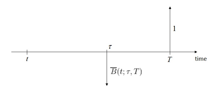
Figure 1: We show the flows that characterize, in the zero-recovery case, a long position on a forward defaultable ZC bond paid at $\tau$ if no default event occurs up to $\tau$. A forward defaultable ZC price is established at time $t$. The contract gives the right to receive $1$ if no default event occurs up to $T$.

In this study we focus on fixed rate coupon bonds that are not callable, puttable, or convertible. A (liquid) corporate coupon bond of the obligor $C$ is

$$\overline{P}(t_{0};{\bf c},{\bf t}):=\sum^{N}_{i=1}c_{i}\overline{B}(t_{0},t_{i})\;.$$ (6)

In the definition of a corporate coupon bond (6), the price depends on the set of flows ${\bf c}:=\{c_{i}\}_{i=1\ldots N}$ and the set of payment dates ${\bf t}:=\{t_{i}\}_{i=1\ldots N}$. We indicate with $T$ the bond maturity, i.e. $t_{N}=T$. The $i^{th}$ payment $c_{i}$ at time $t_{i}$ for ${i<N}$ is the coupon payment with the corresponding daycount, while the last payment at $t_{N}$ has the bond face value added to the coupon payment. A corporate coupon bond $\overline{P}$ always indicates invoice (or dirty) prices, as in standard fixed income modeling.

We indicate with $\overline{P}(t,\tau;{\bf c},{\bf t})$ the forward defaultable coupon bond in $t$ paid in $\tau$ that generalizes the forward defaultable ZC (3) to the case with coupons (6)

$$\overline{P}(t,\tau;{\bf c},{\bf t})=\sum^{N}_{i=1;t_{i}>\tau}c_{i}\frac{\overline{B}(t,t_{i})}{\overline{B}(t,\tau)}\;\;;$$ (7)

where in the forward $\overline{P}(t,\tau;{\bf c},{\bf t})$ only coupons with payment dates $t_{i}>\tau$ appear.

In the next subsection we describe how illiquidity affects corporate coupon bonds (6).

2.2 The sheer liquidity premium

This subsection focuses on the main modeling assumption and it is the core of the approach we propose for pricing illiquid corporate bonds. As already stated in the Introduction, we model illiquidity following closely the option approach of Longstaff (1995). We consider a hypothetical investor who holds, at value date $t_{0}=0$, an illiquid corporate bond. The illiquidity is characterized by one main property: the investor needs some time in order to liquidate a position with a given size of that bond. This hypothetical investor will be able to sell the position in the illiquid bond only after a time-to-liquidate $\tau$ at the same price as a liquid bond with the same characteristics (issuer, coupons, payment dates).

We assume that this investor is an experienced trader better informed than other market players on that particular corporate market segment: this experienced trader knows all the features of the bonds of that issuer and all the potential clients that could be interested in buying the bond he holds.

After the seminal paper of Kyle (1985), the assumption that some market players are better informed than others is rather common when analyzing, from a theoretical perspective, specific trading mechanisms and the price formation process of some assets. In particular, Longstaff’s idea is simple and brilliant: this experienced trader “has perfect market timing ability that would allow him to sell the security and reinvest the proceeds in the riskless asset, at the time $t$ that maximizes the value of his portfolio. […] As long as the investor cannot sell the [illiquid] security prior to time $\tau$, however, he cannot benefit from having perfect market timing ability. (…) [Illiquidity] imposes an important opportunity cost on this hypothetical investor” (cf. Longstaff 1995, pp.1768-1769).

Summarizing, “this incremental cash flow can also be viewed as the payoff from an option” (cf. Longstaff 1995, p.1769). Liquidity is seen as an incremental right (i.e. an option) in the hands of the investor, who can liquidate a given position at market price whenever he desires. The additional value of the liquid security over the illiquid one is calculated by regarding the optimal strategy of this hypothetical investor.

More in detail, two are the differences/specifications of our approach w.r.t. Longstaff (1995), due to the fact that we focus on an illiquid defaultable corporate bond.

First, as an example, Longstaff (1995) focuses his attention on a non-dividend paying stock in IPOs: the value of the asset sold at time $t\in(t_{0},\tau)$ including the reinvestment up to $\tau$ is nothing else than a forward contract in $t$ and expiry in $\tau$ on the asset. In this paper, we follow this approach, dealing with a derivative rather than the underlying asset: the contract we consider is the forward defaultable coupon bond (7) introduced in previous subsection.

Second, we require only an almost perfect market timing for the hypothetical investor. The experienced trader has two relevant pieces of information:

1. he knows whether the corporate will default before $\tau$ (but he does not know exactly when) and

2. in case of no default up to the time-to-liquidate $\tau$, he has perfect market timing ability on the forward defaultable coupon bond before $\tau$.

We return to the plausibility of these hypotheses in the following.

Hence, when dealing with fixed income securities, we have to consider that bonds pay coupons and that they can default. Two are the cases of interest: either the corporate issuer defaults before the time-to-liquidate $\tau$ or it defaults after $\tau$.

In the former case, the illiquid position has a value equal to zero in $\tau$ (and then also in the value date), while the liquid bond is sold immediately at its price at value date $\overline{P}(t_{0};{\bf c},{\bf t})$. This is a consequence of the fact that the hypothetical investor knows that the corporate will default before $\tau$ but he does not know exactly when; he will liquidate his liquid position as soon as possible, while the illiquid one returns zero, due to the zero-recovery of the bond.

In the latter case, the experienced trader sells the liquid position via the forward defaultable coupon bond. It sells this forward with optimal timing, i.e. the selling price is

$$M_{\tau}:=\max_{t_{0}\leq t\leq\tau}\overline{P}(t,\tau;{\bf c},{\bf t})\;\;;$$

this price is received at time $\tau$ (because it is a forward defaultable bond, see also Figure 1). He also sells the illiquid bond in $\tau$ at $\overline{P}(\tau;{\bf c},{\bf t})$. Summing up, the two possibilities for the liquid and illiquid bonds are shown in Table 1.

$$\begin{array}[]{l|cc|l}&liquid&illiquid&\\[2.84526pt] \hline\cr&&&\\[-5.69054pt] t_{d}\leq\tau&\overline{P}(t_{0};{\bf c},{\bf t})&0&\text{received in }t_{0}\\[5.69054pt] t_{d}>\tau&M_{\tau}&\overline{P}(\tau;{\bf c},{\bf t})&\text{received in }\tau\\[5.69054pt] \hline\cr\end{array}$$

Table 1: We show the value of liquid and illiquid bonds for an experienced trader. On the one hand, in case of default before $\tau$ (i.e. $t_{d}\leq\tau$ ) the illiquid bond has no value –due to the zero recovery– while the liquid one is sold immediately at its price in $t_{0}$. On the other hand, in case of default after $\tau$ (i.e. $t_{d}>\tau$ ), the illiquid bond is sold at $\overline{P}(\tau;{\bf c},{\bf t})$ and the liquid position via the forward defaultable coupon bond (with optimal timing): both prices are received in $\tau$.

Longstaff’s idea is very intuitive: the main limitation of holding an illiquid bond, compared with a comparable issue of the same corporate entity, is related to the impossibility for a while to sell the bond and convert its value into cash. The time-to-liquidate $\tau$ is the main exogenous model parameter: it models the liquidity restriction as an opportunity cost for this hypothetical investor. We can now state the main assumption of our modeling set up.

Assumption:

The sheer liquidity premium $\Delta_{\tau}$ is defined as the value at $t_{0}$ of the difference between liquid and illiquid prices of bonds of the same corporate issuer with the same characteristics (same coupons and payments dates). Its present value equals

$$\Delta_{\tau}:=\mathbb{E}\left[{D}(t_{0},\tau)\mathbbm{1}_{t_{d}>\tau}\left(M_{\tau}-\overline{P}(\tau;{\bf c},{\bf t})\right)+\mathbbm{1}_{t_{d}\leq\tau}\overline{P}(t_{0};{\bf c},{\bf t})|{\cal F}_{0}\right]\;.$$ (8)

The sheer liquidity premium is equal to the sum of two terms. As shown in Table 1, the first term, in case of no default up to the time-to-liquidate $\tau$, is equal to the difference, for the hypothetical investor, of the selling prices in $\tau$ of the liquid and illiquid forward defaultable bonds; the second one, in the event of default before $\tau$, is equal to the liquid defaultable bond price in $t_{0}$. $\qquad\diamondsuit\;$

Let us discuss the plausibility of the above assumption and the role of the experienced trader.

The experienced trader closely models some real market makers that operate in the corporate bond market. Within this market some market makers, often within major dealers, are very specialized on few issuers and sometimes only on few issues of a given issuer. On the corporate side, these traders often know personally the top-management of the firm, its liquidity needs, its funding policy, the next issues in the primary market. On the market side, they know in detail the market segment where they operate, every relevant investor who has invested on that corporate or who can be interested to that firm name, they advise the company to obtain financing in the primary market overseeing primary bond sales to investors in that company or in strictly related firms.

As previously mentioned, two are the main hypotheses on the experienced trader related to i) the knowledge of the arrival of a default before $\tau$ and ii) the perfect timing ability in case of no default before $\tau$. Both hypotheses sound reasonable for market makers who have access to the soft information we have described above.

Moreover, something can be said on the first hypothesis; it can be useful to remember that the time-to-liquidity is few months in the most illiquid cases and some days or weeks more generally, and most of the trading activity on illiquid corporate bonds is concentrated on issuers either investment grade or with the highest ratings in the speculative grade. Within such a short time interval (compared to the typical maturity of corporate issues), it sounds reasonable –for this class of market makers– to know with high-probability whether the corporate issuer would default or not in the (rare) event of issuer default before the time-to-liquidate; it is instead rather improbable that they know exactly when.

The second hypothesis is the same as Longstaff’s one, under the condition of no-default before $\tau$.

For sure, in the corporate bond market, asymmetric information helps these market makers in the selection of market timing, where higher prices are mainly due to a renewed interest on a specific firm related to, e.g., a change in its financing policy, new issues in the primary market or unexpected reported results by the corporate. It is also sure that this information sounds more valuable in a market, as the corporate bond one, where market abuse is extremely difficoult to detect.

Having said that, though the experienced trader is an idealization. As already stated by Longstaff, the sheer liquidity premium $\Delta_{\tau}$ “would be less for an actual investor with imperfect market timing ability. Thus, the present value of the incremental cash flow represents an upper bound on the value of marketability”(cf. Longstaff 1995, p.1769).

Remark. The above definition does not consider the case when coupon payments take place between the value date $t_{0}$ and $\tau$. We have already underlined that the time-to-liquidate is, even in the most illiquid cases, a few months, and then at most one coupon payment could be present in the time interval $(t_{0},\tau)$. The first coupon, when paid before $\tau$, can be separated by the other flows in the coupon bond; a technique known in the market place as coupon stripping. In practice, corporate bond traders consider that payment, i.e. within a short lag in the future, very liquid. We assume that this coupon makes the same contribution to both the liquid and illiquid coupon bonds, i.e. it maintains only its interest rate and credit risk components; thus, this coupon does not appear in the sheer liquidity premium $\Delta_{\tau}$ in (8). Hereinafter, we consider in the corporate coupon bond only the coupons after the time-to-liquidate, i.e. in definition (6) the first coupon in the sum is the first one paid after $\tau$.

2.3 A parsimonious model selection

It can be interesting to observe that, within the DHJM framework, the sheer liquidity premium (8) can be written in a simpler form

$$\begin{split}\Delta_{\tau}&=\overline{B}(t_{0},\tau)\,\mathbb{E}^{(\overline{\tau})}\left[M_{\tau}|{\cal G}_{0}\right]-\mathbb{P}(t_{0},\tau)\,\overline{P}(t_{0};{\bf c},{\bf t})\;\;,\end{split}$$ (9)

where $\mathbb{P}(t_{0},\tau)$ is the issuer survival probability up to the time-to-liquidate (for a deduction of this simple equality within DHJM, see also (21) in Appendix A). Let us notice that the first term of (9) is the only quantity in the price of illiquidity $\Delta_{\tau}$ rather complicated to be computed: it depends on $\overline{r}_{t}$ and not separately on $r_{t}$ and $\lambda_{t}$.

This property holds whichever zero-recovery DHJM model is selected (i.e. whatever $\sigma(t,T)$ and $\overline{{\sigma}}(t,T)$ are chosen) for the dynamics (2) of $B(t,T)$ and $\overline{B}(t,T)$. As discussed in the Introduction, the main driver for model selection is parsimony when dealing with illiquid corporate bonds, due to the poorness of the data set and model calibration issues. One of the simplest and most parsimonious models within DHJM was proposed by Schönbucher (2000), where both $r_{t}$ and $\lambda_{t}$ follow two correlated 1-dimensional Hull and White (1990) models

$$\left\{\begin{array}[]{lcl}r_{t}&=&\varphi_{t}+x^{(1)}_{t}\\ \lambda_{t}&=&\psi_{t}+x^{(2)}_{t}\end{array}\right.$$

where $x^{(1)}_{t}$ and $x^{(2)}_{t}$ are two correlated Ornstein–Uhlenbeck processes (OU) with zero mean and zero initial value; $\varphi_{t}$ and $\psi_{t}$ are two deterministic functions of time. This model has the main advantage of allowing an elementary separate calibration of the zero-rates (via $\varphi_{t}$) and the Zeta-spread curve (via $\psi_{t}$) at value date $t_{0}$. A consequence of the observation that only the dynamics for $\overline{r}_{t}$ matters for liquidity, makes us consider an even simpler model with the two OU perfectly correlated, i.e. with only one OU driver, as recently proposed by Baviera (2019) in a multi-curve problem.

In this case, the risk-free interest rate $r_{t}$ and the intensity $\lambda_{t}$ are modeled as

$$\left\{\begin{array}[]{lcl}r_{t}&=&\varphi_{t}+(1-{\hat{\gamma}})\;x_{t}\\ \lambda_{t}&=&\psi_{t}+{\hat{\gamma}}\;x_{t}\end{array}\right.$$ (10)

with $x_{t}$ an OU with zero mean and initial value

$$\left\{\begin{array}[]{lcl}dx_{t}&=&-{\hat{a}}\,x_{t}\,dt+{\hat{\sigma}}\,dW_{t}\\ x_{0}&=&0\end{array}\right.$$

where ${\hat{\gamma}}\in[0,1]$, while $\hat{a},\hat{\sigma}$ are two positive constant parameters.

This model selection is in line with day-to-day practice. In the marketplace, often one cannot observe options that allow calibrating separately the volatility of the risk-free curve and the volatility of the credit spread, i.e. there is not enough information to discriminate between the two dynamics. One can associate a fraction ${\hat{\gamma}}$ of the total dynamics to the credit component and the remaining fraction to the interest rate component. Conversely, the two initial curves (risk-free zero-rate and Zeta-spread) can be easily calibrated separately on market data and the integrals of $\varphi_{t},\psi_{t}$ between $t_{0}$ and a given maturity $T$ are related to these two curves up to $T$. We provide final formulas in terms of $B(t_{0},T)$ and $\overline{B}(t_{0},T)$ because both curves can be calibrated directly from market data.

A consequence of (10) is that the defaultable rate $\overline{r}_{t}=r_{t}+\lambda_{t}$ is

$$\overline{r}_{t}=\varphi_{t}+\psi_{t}+x_{t}\;\;.$$

It is modeled according to a Hull–White model with one-dimensional volatility (see, e.g. Brigo and Mercurio 2007)

$$\overline{\sigma}(t,T)=\frac{\hat{\sigma}}{\hat{a}}\left(1-e^{-{\hat{a}}(T-t)}\right)\,\in\,\Re\qquad t\leq T\,$$ (11)

and then the volatility $v(t;\tau,t_{i})=\overline{{\sigma}}(t,t_{i})-\overline{{\sigma}}(t,\tau)$, defined in equation (5), is a separable function in the times $t$ and $t_{i}$, i.e.

$$v(t;\tau,t_{i})=\zeta_{i}\,\nu(t)$$ (12)

with $\zeta_{i}:=(\hat{\sigma}/\hat{a})\left[1-e^{-\hat{a}(t_{i}-\tau)}\right]$ and $\nu(t):=e^{-\hat{a}(\tau-t)}$ with $t_{0}\leq t\leq\tau\leq t_{i}$.

In the next section we show that, with the proposed model (10), it is possible to compute the sheer liquidity premium $\Delta_{\tau}$ (9) via a closed formula and it is possible to associate a liquidity spread as a component of the corporate bond spread in addition to the credit spread.

3 A closed formula for illiquid corporate coupon bonds

In this section we present the main result of this paper: the sheer liquidity premium $\Delta_{\tau}$ (9) can be evaluated directly via a simple closed formula obtained using valuation techniques from option-pricing theory.

This result is far from being obvious. A forward defaultable coupon bond $\overline{P}(t,\tau;{\bf c},{\bf t})$ is the sum of forward defaultable ZCs $\{\overline{B}(t;\tau,t_{i})\}_{i=1\ldots N}$, each one following the dynamics (4) and then described as a Geometric Brownian Motion (GBM) in the case of deterministic volatilities (11) we are considering. No known closed formula exists for the running maximum of a sum of GBMs.

In order to get the closed formula, we take the following steps. First, we consider a lower and an upper bound of (8) that can be computed via closed formulas. Then, we show, calibrating the model parameters for two European issuers, that the difference between the upper and lower bounds is negligible for all practical purposes. We can then use one of the two bounds as the closed-form solution we are looking for; in this section we present these bounds and in the next section we show the tightness of their difference.

Lower and upper bounds for the sheer liquidity premium $\Delta_{\tau}$ (8) are:

$$\sum_{i=1}^{N}c_{i}\overline{B}(t_{0},t_{i})\left(\pi^{L}_{i}(\tau)-\mathbb{P}(t_{0},\tau)\right)\leq\Delta_{\tau}\leq\sum_{i=1}^{N}c_{i}\overline{B}(t_{0},t_{i})\left(\pi^{U}_{i}(\tau)-\mathbb{P}(t_{0},\tau)\right)$$ (13)

where the sum is limited to the payment dates $t_{i}>\tau$ and

$$\begin{array}[]{lcl}\pi^{U}_{i}(\tau)&:=&{\displaystyle\frac{4+\Sigma^{2}_{i}(\tau)}{2}\,\Phi\left(\frac{\Sigma_{i}(\tau)}{2}\right)+\frac{\Sigma_{i}(\tau)}{\sqrt{2\pi}}\,\exp\left(-\frac{\Sigma_{i}^{2}(\tau)}{8}\right)}\\[11.38109pt] \pi^{L}_{i}(\tau)&:=&{\displaystyle\int^{1}_{0}d\eta\frac{e^{-\frac{1}{8}\Sigma^{2}_{N}(\tau)}}{\pi\,\sqrt{1-\eta}\,\sqrt{\eta}}\,e^{-\frac{\eta}{2}\,\Sigma_{i}(\tau)\,\left(\Sigma_{i}(\tau)-\Sigma_{N}(\tau)\right)}}\\[8.53581pt] &&\;\;{\displaystyle\left\{1+\sqrt{\frac{\pi\,(1-\eta)}{2}}\,\Sigma_{N}(\tau)\,e^{\frac{1-\eta}{8}\,\Sigma^{2}_{N}(\tau)}\,\Phi\left[\frac{\sqrt{1-\eta}}{2}\,\Sigma_{N}(\tau)\right]\right\}}\\[8.53581pt] &&\;\;{\displaystyle\left\{1+\sqrt{\frac{\pi\,\eta}{2}}\,\left(2\,\Sigma_{i}(\tau)-\Sigma_{N}(\tau)\right)\,e^{\frac{\eta}{8}\,\left(2\,\Sigma_{i}(\tau)-\Sigma_{N}(\tau)\right)^{2}}\,\Phi\left[\frac{\sqrt{\eta}}{2}\,\left(2\,\Sigma_{i}(\tau)-\Sigma_{N}(\tau)\right)\right]\right\}}\end{array}$$ (14)

The cumulated volatility is

$$\Sigma^{2}_{i}(\tau):=\displaystyle\int^{\tau}_{t_{0}}v^{2}(s;\tau,t_{i})\,ds=\zeta_{i}^{2}\,\frac{1-e^{-2\hat{a}\tau}}{2\hat{a}}$$

where $\zeta_{i}$ is defined in equation (12), $\Phi[\bullet]$ is the standard normal CDF and the issuer survival probability up to the time-to-liquidate is

$$\mathbb{P}(t_{0},\tau)=\exp\left\{{-\int^{\tau}_{t_{0}}\psi_{s}ds+\frac{\hat{\gamma}^{2}}{2}\int^{\tau}_{t_{0}}\overline{\sigma}^{2}(s,\tau)\,ds}\right\}\;,$$ (15)

with $\psi_{s}$ the deterministic part of the intensity introduced in (10) and $\overline{\sigma}(s,\tau)$ is defined in (11).

The bounds for the sheer liquidity premium $\Delta_{\tau}$ (13) are the key theoretical result of this paper: the interested reader can found the deduction of these inequalities in Appendix C. In Section 4 we show for two issuers that these bounds appear to be very tight, being their difference on the order of $10^{-8}$ the face value in the worst case (i.e., in Euro terms, it corresponds to €$1$ every €$100$ million): it can be considered negligible for all practical purposes.

In practice, either of the two closed form solutions (lower or upper bound) can be used indifferently, and in particular, the simplest expression of the two bounds, i.e. the upper bound. This fact allows defining, in an elementary way, a sheer liquidity spread as done in the next subsection.

3.1 The sheer liquidity spread

A consequence of equation (13) and of the tightness of the difference between the two bounds is that the illiquid corporate coupon price is

$$\overline{\overline{P}}_{\tau}(t_{0};{\bf c},{\bf t}):=\overline{P}(t_{0};{\bf c},{\bf t})-\Delta_{\tau}=\sum^{N}_{i=1}c_{i}\overline{B}(t_{0},t_{i})\,\left(1+\mathbb{P}(t_{0},\tau)-\pi^{U}_{i}(\tau)\right)$$ (16)

where $\pi^{U}_{i}(\tau)$ is defined in (14) and the survival probability $\mathbb{P}(t_{0},\tau)$ can be found in (15). We can also define an illiquid ZC as

$$\overline{\overline{B}}_{\tau}(t_{0},t_{i}):=\overline{B}(t_{0},t_{i})\,\left(1+\mathbb{P}(t_{0},\tau)-\pi^{U}_{i}(\tau)\right)\;\;$$

and its sheer liquidity spread as

$$L_{\tau}(t_{i}):=-\frac{1}{t_{i}-t_{0}}\ln\frac{\overline{\overline{B}}_{\tau}(t_{0},t_{i})}{\overline{B}(t_{0},t_{i})}=-\frac{1}{t_{i}-t_{0}}\ln\left(1+\mathbb{P}(t_{0},\tau)-\pi^{U}_{i}(\tau)\right)\;\;.$$ (17)

Thus, we can decompose the illiquid ZC bond into three components: risk-free discount, credit, and liquidity:

$$\overline{\overline{B}}_{\tau}(t_{0},T)=\underbrace{e^{-R(T)(T-t_{0})}}_{risk-free}\;\underbrace{e^{-Z(T)(T-t_{0})}}_{credit}\;\underbrace{e^{-L_{\tau}(T)(T-t_{0})}}_{liquidity}$$

where $R(T)$ is the Zero rate and $Z(T)$ is the Zeta spread of the liquid bond. This corresponds to the idea of Jarrow (2001) where liquidity is seen as a component in bond yield in addition to the default risk component; it is also in line with the practice of market makers in their day-to-day activities: they add to the bond credit spread a basis related to liquidity.

It is useful to underline that the sheer liquidity spread $L_{\tau}(t_{i})$ in (17) is not affected by the rate component and is affected only slightly by the credit component: this property suits its name (sheer). The liquidity component in the ZC price $L_{\tau}(t_{i})$ is function of $\left(1+\mathbb{P}(t_{0},\tau)-\pi^{U}_{i}(\tau)\right)$, thus it depends mainly on the cumulated volatility $\Sigma_{i}(\tau)$, because – as we’ll show in the numerical examples – the quantity $1-\mathbb{P}(t_{0},\tau)$ is two orders of magnitude smaller than $1-\pi^{U}_{i}(\tau)$.

Let us stress a relevant result of the theoretical formulation presented in this study. It allows identifying the two key risk factors in the liquidity spread: the volatility of the corresponding liquid bond and the time-to-liquidate.

4 An application to the financial sector in the European bond market

In this section we illustrate the impact of illiquidity applying formula (16) to obligations with different maturities issued by two main financial institutions in Europe. We also show that the difference between the upper and lower bounds of the illiquidity premium is negligible for all practical purposes.

4.1 Calibration of model parameters

The two European financial institutions in Europe that we consider in this study are BNP Paribas S.A. (hereinafter BNPP) and Banco Santander S.A. (Santander) on 10 September 2015 (value date). The settlement date is 14 September 2015. At value date, BNPP was rated A and Santander A- according to S&P.

maturity	coupon (%)	clean price
27-Nov-2017	2.875	105.575
12-Mar-2018	1.500	102.768
21-Nov-2018	1.375	102.555
28-Jan-2019	2.000	104.536
23-Aug-2019	2.500	106.927
13-Jan-2021	2.250	106.083
24-Oct-2022	2.875	110.281
20-May-2024	2.375	106.007

Table 2: Clean prices for BNPP liquid bonds. Senior unsecured benchmark issues with maturity less than or equal to $10$ years. Coupons are annual with day-count convention Act/Act. Prices are end-of-day mid-prices on 10 September 2015.

maturity	coupon (%)	clean price
27-Mar-2017	4.000	105.372
04-Oct-2017	4.125	107.358
15-Jan-2018	1.750	102.766
20-Apr-2018	0.625	99.885
14-Jan-2019	2.000	103.984
13-Jan-2020	0.875	99.500
24-Jan-2020	4.000	112.836
14-Jan-2022	1.125	98.166
10-Mar-2025	1.125	93.261

Table 3: Clean prices for Santander senior unsecured benchmark issues with maturity less than or equal to $10$ years. Coupons are annual with day-count convention Act/Act. Prices are end-of-day mid-prices at value date.

As discussed in Section 3, the closed formula for illiquid bond prices, besides the bond characteristics (maturity, payment dates, coupons, sinking features, time-of-liquidate, etc…), includes the observed i) zero-rate curve, ii) credit spread term-structure for the issuer of interest, and iii) bond volatility. These “ingredients” can be calibrated with the market data following standard techniques.

First, the risk-free curve we consider is the OIS curve as the market standard; it has been bootstrapped from OIS quoted rates. Quotes at value date are provided by Bloomberg. The discount curve $B(t_{0},T)$ is bootstrapped following the standard procedure; OIS rates and discount factors are reported in Baviera (2019).

Second, in order to construct the Zeta-spread curve, i.e. the (liquid) credit component in the spread, we consider all senior unsecured benchmark issues (i.e. with issue size larger than €$500$ million) with maturity less than or equal to $10$ years. Coupons are paid annually with the Act/Act day-count convention for all bonds in both sets. The closing day mid-prices are reported in Tables 2 and 3.

For each one of the two issuers, its time-dependent Zeta-spread curve

$$Z(T):=-\frac{1}{T-t_{0}}\ln\frac{\overline{B}(t_{0},T)}{B(t_{0},T)}\;\;$$

can be bootstrapped from liquid bond invoice prices (see, e.g. Schönbucher 2003). Invoice prices are obtained adding the accrual to the clean prices in Tables 2 and 3. We assume a constant Zeta-spread curve up to the maturity of the bond with the lowest maturity and we use a linear interpolation rule on Zeta-spread afterwards; the day-count convention for Zeta-spreads is Act/365, as the market standard.

Finally, the volatility parameters ($\hat{a}$, $\hat{\sigma}$ and $\hat{\gamma}$) should be calibrated on options on corporate bonds. Unfortunately, prices on liquid options on BNPP and Santander bonds are not available in the market at value date. We consider a proxy in order to calibrate the volatility parameters; we notice that at value date both banks are Systemically Important Financial Institutions (SIFI) and belong to the panel of banks contributing to the Euribor rate. The dynamics of the spread between the Euribor and the OIS curve can be considered a good proxy of the dynamics of the average credit spread for financial institutions with the above characteristics. As mentioned in Grbac and Runggaldier (2015), this spread models the risk related to the Euro interbank market, and default risk is one important component of this interbank risk. Let us underline that we use this proxy to calibrate only volatility parameters, while credit spreads are calibrated on issuer liquid bond market.

ATM swaptions on Euribor swap rates are very liquid in Europe: we can use these OTC option contracts at $t_{0}$ as a proxy, in order to calibrate the volatility parameters. Swaption ATM normal volatilities are provided by Bloomberg; their values in $t_{0}$ and the calibration procedure are reported in Baviera (2019). Calibrated values are $\hat{a}=12.94\%$, $\hat{\sigma}=1.26\%$ and $\hat{\gamma}=0.07\%$.

In the two cases analyzed, as already mentioned in Section 2, the correction to include the default risk up to ttl is small. All survival probabilities $\mathbb{P}(t_{0},\tau)$ are close to $1$: we report in Table 4 the default probabilities $1-\mathbb{P}(t_{0},\tau)$ in the time interval of interest. All values are of order $10^{-4}$.

	BNPP	Santander
2w	$1.27\times 10^{-4}$	$1.80\times 10^{-4}$
2m	$5.42\times 10^{-4}$	$7.73\times 10^{-4}$

Table 4: Default probabilities $1-\mathbb{P}(t_{0},\tau)$ for BNPP and Santander for the two ttl of $2$ weeks and $2$ months.

The correction due to the default risk up to ttl is negligible in the liquidity spread: this fact justifies the decomposition of the bond spread in the three components risk-free, credit and liquidity proposed in Section 3.1 and the adjective (sheer) of the liquidity spread we consider.

4.2 Illiquid bond prices

In this section we show that, considering two sets of illiquid bonds with the same characteristics as the liquid bonds (e.g. coupons and payments dates) and ttl equal to either two weeks or two months, the difference between the lower and upper bounds for the sheer liquidity premium $\Delta_{\tau}$ is on the order of $10^{-8}$ times the face value. Figure 2 presents this difference for BNPP, and Figure 3 for Santander. This difference is the maximum error we make if we evaluate $\Delta_{\tau}$ with one of these bounds. It is negligible for all practical purposes.

Figure 2: Difference between the upper and lower bounds for the sheer liquidity premium $\Delta_{\tau}$ for BNPP bonds. We consider illiquid bonds with the same characteristics (e.g. coupons, payment dates) as the bonds in Table 2 with ttl equal to two weeks (continuous blue line and squares) and two months (dashed red line and triangles). This difference is on the order of $10^{-8}$ times the face value in the worst-case, and so it is negligible for all practical purposes.

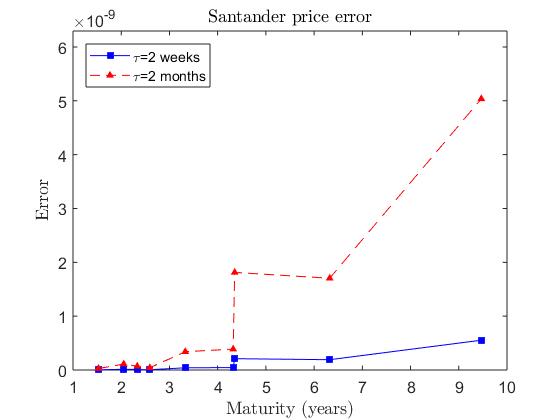
Figure 3: Difference between the upper and lower bounds for the sheer liquidity premium $\Delta_{\tau}$ for Santander bonds. We consider illiquid bonds with the same characteristics (e.g. coupons, payment dates) as the bonds in Table 3 with ttl equal to two weeks (continuous blue line and squares) and two months (dashed red line and triangles). This difference is on the order of $10^{-9}$ times the face value.

Moreover, as a robustness test, we have considered this difference between the two bounds for a wide range of volatility parameters around the estimated values, keeping equal all other bond characteristics: $\hat{a}\in(0,30\%)$, $\hat{\sigma}\in(0,4\%)$ and $\hat{\gamma}\in(0,0.2\%)$. We observe that this difference is, in the worst case, less than $1$ Euro for every million of face value. Again, we find that the difference between the two bounds is negligible for all practical purposes. This fact allows us to consider indifferently either the lower or the upper bound in (14) as a closed-form solution for $\Delta_{\tau}$.

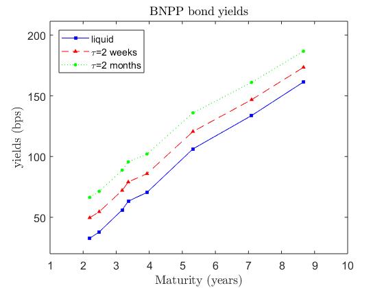
Figure 4: BNPP bond yields. We consider all benchmark issues with maturity less than 10y described in Table 2 and their yields (continuous blue line and squares). We show also the yield obtained for illiquid bonds with the same characteristics (e.g. coupons, payment dates) with ttl equal to two weeks (dashed red line and triangles) and two months (dotted green line and circles).

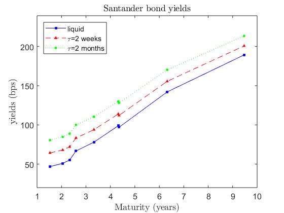
Figure 5: Santander bond yields. We consider all benchmark issues with maturity lower than 10y in Table 3 and their yields (continuous blue line and squares). We show also the yield obtained for illiquid bonds with the same characteristics (e.g. coupons, payment dates) with ttl equal to two weeks (dashed red line and triangles) and ttl equal to two months (dotted green line and circles).

In Section $3$ we have shown that a sheer liquidity spread (17) could be added to each ZC in order to take into account liquidity. Practitioners often consider a liquidity yield spread as the term that should be added to the yield in order to obtain the illiquid bond price (16)

$$\overline{\overline{P}}_{\tau}(t_{0},T;{\bf c},{\bf t})=:\sum^{N}_{i=1}c_{i}\;e^{-\left[{\cal Y}(T)+{\cal L}_{\tau}(T)\right]\,(t_{i}-t_{0})}$$

where ${\cal Y}(T)$ is the yield of the corresponding liquid bond $\overline{P}(t_{0};{\bf c},{\bf t})$ and ${\cal L}_{\tau}(T)$ the liquidity yield spread for ttl equal to $\tau$.

In Figures 4 and 5 we show the liquidity yield spread for BNPP and Santander for different bond maturities and ttl equal to two weeks and two months. We observe that, for the same time-to-liquidate $\tau$, the liquidity yield spread ${\cal L}_{\tau}(T)$ depends only slightly on bond maturity $T$.

5 Conclusions

In this paper we have proposed an approach via a reduced-form model for pricing illiquid corporate bonds when the corresponding liquid bonds are observed in the market. It allows a closed formula (16) for illiquid bond prices when they are not available in the marketplace and a direct calibration of parameters on the risk-free curve, the Zeta-spread curve of the issuer of interest and its bond volatility. We have shown a detailed model calibration for two European corporate issuers in the financial sector.

Our approach models the difference between liquid and illiquid coupon bond prices, named sheer liquidity premium, as a right in investor hands. The formula is deduced in two steps: i) bounding from above and below the sheer liquidity premium (8) in a DHJM (10) and ii) showing the equivalence of these two bounds for all practical purposes.

This closed formula (16) is simple and allows to identify the two key drivers of the sheer liquidity: the bond volatility and the “time-to-liquidate” a given bond position. It can be used by practitioners for different possible applications. Let us mention some of them.

This model can support market makers in their day-to-day activities. On the one hand, the ttl parameter can be evaluated ex ante by an experienced trader with a deep knowledge of the characteristics of that particular illiquid market (concentration, frequency for trades with similar characteristics observed in the recent past) who desires to liquidate a given position; the formula gives a theoretical background for the market practice of adding a liquidity spread to the bond yields either when pricing illiquid issues or when receiving them as collateral. On the other hand, the formula can also be used to obtain an “implied time-to-liquidate” from market quotes if both liquid and illiquid prices are available, translating observable spreads into a time lag for liquidating a position and hence providing an interesting piece of information for market participants.

Moreover, the model can be useful also to risk managers. By offering an explicit relationship between the bond volatility and the sheer liquidity premium, it offers to risk managers a way to justify the market practice of setting limits on illiquid bond positions based on the volatility of similar liquid bonds and it gives a theoretical background for haircuts of illiquid bonds accepted as collateral. Moreover, the ttl can be backtested ex post by risk managers, who, thanks to the transaction data made recently available, can measure the average time needed for liquidating a position in an illiquid corporate bond of a given size.

The proposed approach clarifies that illiquidity is an intrinsic component of the bond spread mainly related to the cumulated volatility. In the presence of a liquid credit curve, it allows to disentangle the two components, credit and liquidity, in the observed spread over the risk free rate.

Notation and Shorthands

Shorthands

$$\begin{array}[]{lcl}{\rm CDF}&:&{\rm Cumulative\;Distribution\;Function}\\[2.84526pt] {\rm cf.}&:&{\rm compare;\;from\;Latin:\;confer}\\[2.84526pt] {\rm FR}&:&\text{fractional-recovery (model)}\\[2.84526pt] {\rm DHJM}&:&\text{Defaultable HJM framework}\\[2.84526pt] {\rm GBM}&:&\text{Geometric Brownian Motion}\\[2.84526pt] {\rm IPO}&:&\text{Initial Public Offering}\\[2.84526pt] {\rm MiFID}&:&\text{Markets in Financial Instruments Directive}\\[2.84526pt] {\rm OTC}&:&\text{Over The Counter}\\[2.84526pt] {\rm OU}&:&\text{Ornstein--Uhlenbeck process}\\[2.84526pt] {\rm pdf}&:&{\rm probability\;density\;function}\\[2.84526pt] {\rm s.t.}&:&{\rm such\;that}\\[2.84526pt] {\rm ttl}&:&\text{time-to-liquidate}\\[2.84526pt] {\rm w.r.t.}&:&{\rm with\;respect\;to}\\[2.84526pt] {\rm TRACE}&:&\text{Trade Reporting and Compliance Engine}\\[2.84526pt] {\rm ZC}&:&\text{zero-coupon bond}\\[2.84526pt] \end{array}\;\;.$$

Notation

Symbol	Description
${\hat{a}},{\hat{\sigma}},{\hat{\gamma}}$	parameters in short rate $r_{t}$ and intensity $\lambda_{t}$ dynamics (10)
$B(t,T)$	risk-free zero-coupon (ZC) bond at $t$ with maturity $T$
${\overline{B}}(t,T)$	defaultable ZC bond at $t$ with maturity $T$ and zero-recovery
$\overline{\overline{B}}_{\tau}(t,T)$	illiquid defaultable ZC bond at $t$ with maturity $T$ , zero-recovery and ttl equal to $\tau$
${\overline{B}}(t;\tau,T)$	forward ZC bond
${\bf c}=\{c_{i}\}_{i=1,\ldots,N}$	defaultable coupon bond flows (coupons and face value)
$\overline{P}(t_{0};{\bf c},{\bf t})$	defaultable coupon bond at $t_{0}$
$\overline{\overline{P}}_{\tau}(t_{0};{\bf c},{\bf t})$	illiquid defaultable coupon bond at $t_{0}$ with ttl equal to $\tau$
$\overline{P}(t,\tau;{\bf c},{\bf t})$	forward defaultable coupon bond at $t$, paid at $\tau$
$\mathbb{P}(t_{0},\tau)$	corporate issuer survival probability up to the time-to-liquidate $\tau$
$\Delta_{\tau}$	sheer liquidity premium with ttl equal to $\tau$
${D}(t,T)$	stochastic discount factor, equal to $\displaystyle\exp\left(-\int^{T}_{t}r_{s}\,ds\right)$
${\overline{D}}(t,T)$	defaultable stochastic discount factor, equal to $\displaystyle\exp\left(-\int^{T}_{t}\overline{r}_{s}\,ds\right)$
$\mathbb{E}[\bullet]\;\&\;\mathbb{E}^{(\overline{\tau})}[\bullet]$	expectation under the risk neutral & under the $\tau$-defaultable-forward measure
$L_{\tau}(t_{i})$	sheer liquidity spread for a ZC with maturity $t_{i}$ and ttl $\tau$
${\cal L}_{\tau}(T)$	liquidity yield spread for a coupon bond with maturity $T$ and ttl $\tau$
$N$	number of coupons in the defaultable bond
${\cal N}_{t}$	Cox process with stochastic intensity $\lambda_{t}$ that models default of the corporate issuer
$q$	loss fraction given default in FR models; $q=1^{-}$ reproduces the zero-recovery case
$\lambda_{t}$	stochastic intensity at time $t$
$r_{t}$	risk-free short rate at time $t$
$\overline{r}_{t}$	defaultable short rate at time $t$, defined as $r_{t}+q\lambda_{t}$
$\rho$	instantaneous correlation matrix in $\Re^{d\times d}$ s.t. $dW^{(i)}_{t}\;dW^{(j)}_{t}=\rho_{i\,j}\,dt$
$\sigma(t,T)\,\&\,\overline{\sigma}(t,T)$	DHJM risk-free and defaultable ZC volatilities between $t$ and $T$ in $\Re^{d}$
$\Sigma_{i}(\tau)$	cumulated volatility s.t. $\Sigma^{2}_{i}(\tau):=\displaystyle\int^{\tau}_{t_{0}}v^{2}(s;\tau,t_{i})\,ds$
$t_{0}$	value date ($t_{0}=0$)
$t_{d}$	time to default
$\tau$	time-to-liquidate (ttl)
${\bf t}=\{t_{i}\}_{i=1,\ldots,N}$	payment dates of the defaultable coupon bond with maturity $t_{N}\equiv T$
$v(t;\tau,T)$	equal to $\sigma(t,T)-\sigma(t,\tau)$
$W_{t}$	vector of correlated Brownian motions in $\Re^{d}$ s.t. $dW^{(i)}_{t}\;dW^{(j)}_{t}=\rho_{i\,j}\,dt$
$x\cdot y$	scalar product between $x,y\in\Re^{d}$
$x^{2}$	an abbreviation for scalar product $x\cdot\rho x$ with $x\in\Re^{d}$ and $\rho\in\Re^{d\times d}$ correlation
${\cal Y}(T)$	yield of the corporate bond $\overline{P}(t_{0};{\bf c},{\bf t})$ with maturity $T$

Appendix A

In this Appendix we recall some basic properties of DHJM with fractional recovery (see, e.g. Duffie and Singleton 1999, Schönbucher 1998). We also show an application of these properties to the price of illiquidity (8).

Absence of arbitrage require that the instantaneous risk-free rate $r_{t}$ and the defaultable one $\overline{r}_{t}$ satisfy

$$\left\{\begin{array}[]{rcl}r_{t}&:=&{\displaystyle-\frac{\partial\ln B(t_{0},t)}{\partial t}+\frac{1}{2}\int^{t}_{t_{0}}\frac{\partial}{\partial t}\sigma(s,t)^{2}\;ds-\int^{t}_{t_{0}}\frac{\partial}{\partial t}\sigma(s,t)\cdot dW_{s}}\\[11.38109pt] \overline{r}_{t}&:=&{\displaystyle-\frac{\partial\ln\overline{B}(t_{0},t)}{\partial t}+\frac{1}{2}\int^{t}_{t_{0}}\frac{\partial}{\partial t}\overline{\sigma}(s,t)^{2}\;ds-\int^{t}_{t_{0}}\frac{\partial}{\partial t}\overline{\sigma}(s,t)\cdot dW_{s}}\;,\end{array}\right.$$ (18)

that correspond to equations (25) and (17) in (Schönbucher 1998), with $\overline{B}(t_{0},t)=\overline{B}_{q}(t_{0},t)\;\forall t$.

The above dynamics for $\overline{r}_{t}$ implies that, at value date $t_{0}$, the relation between defaultable discount and defaultable ZC is

$$\overline{D}_{q}(t_{0},\tau)=\overline{B}(t_{0},\tau)\exp\left\{-\frac{1}{2}\int^{\tau}_{t_{0}}\overline{{\sigma}}^{2}(s,\tau)\;ds+\int^{\tau}_{t_{0}}\overline{{\sigma}}(s,\tau)\cdot d{W}_{s}\right\}\;.$$ (19)

This relation is the same of the one in the HJM for risk-free rates, because all quantities are continuous (see, e.g. Musiela and Rutkowski 2006). A consequence of equation (19) is that the $\overline{\tau}$-forward measure presents an interesting property at value date $t_{0}=0$

$$\mathbb{E}\left[\overline{D}_{q}(t_{0},\tau)\;\bullet\;|{\cal G}_{0}\right]=\overline{B}(t_{0},\tau)\;\mathbb{E}^{(\overline{\tau})}\left[\;\bullet\;|{\cal G}_{0}\right]$$ (20)

that is an application of Girsanov’s theorem (see, e.g. Musiela and Rutkowski 2006).

Moreover, from equations (2) we get that the value of the defaultable ZC at a generic time $t$ starting from the initial condition in $t_{0}$ is

$$\overline{B}(t,T)=\overline{B}(t_{0},T)\;(1-q)^{{\cal N}_{t}}\;\exp\left\{\int^{t}_{t_{0}}\left[\overline{r}_{s}-\frac{1}{2}\overline{{\sigma}}^{2}(s,T)\right]ds+\int^{t}_{t_{0}}\overline{{\sigma}}(s,T)\cdot d{W}_{s}\right\}\;.$$

which can be obtained using the Generalized Itô lemma (see, e.g. Schönbucher 1998, eq.(79) p.185). Thus, the default of $\overline{B}_{q}(t,T)$ occurs when the process jumps. In case of a jump at time $t$, the jump size is

$$\Delta\overline{B}_{q}(t,T)=\overline{B}_{q}(t,T)-\overline{B}_{q}(t^{-},T)=-\overline{B}_{q}(t^{-},T)\,q\,d{\cal N}_{t}$$

i.e. the ZC loses a fraction $q$ of its pre-default value, as indicated when introducing the model in (1).

Finally, we show that, within the DHJM framework with $q=1^{-}$, the price of illiquidity (8) can be simplified

$$\begin{split}\Delta_{\tau}&=\mathbb{E}\left[\overline{D}(t_{0},\tau)M_{\tau}|{\cal G}_{0}\right]-\mathbb{E}\left[\overline{D}(t_{0},\tau)\overline{P}(\tau;{\bf c},{\bf t})|{\cal G}_{0}\right]+\left(1-\mathbb{P}(t_{0},\tau)\right)\overline{P}(t_{0};{\bf c},{\bf t})=\\ &=\overline{B}(t_{0},\tau)\left\{\mathbb{E}^{(\overline{\tau})}\left[M_{\tau}|{\cal G}_{0}\right]-\mathbb{E}^{(\overline{\tau})}\left[\overline{P}(\tau;{\bf c},{\bf t})|{\cal G}_{0}\right]\right\}+\left(1-\mathbb{P}(t_{0},\tau)\right)\overline{P}(t_{0};{\bf c},{\bf t})=\\ &=\overline{B}(t_{0},\tau)\,\mathbb{E}^{(\overline{\tau})}\left[M_{\tau}|{\cal G}_{0}\right]-\mathbb{P}(t_{0},\tau)\,\overline{P}(t_{0};{\bf c},{\bf t})\;\;,\end{split}$$ (21)

where $\mathbb{P}(t_{0},\tau)$ is the issuer survival probability up to the time-to-liquidate. The first line comes from iterated expectation, the second line is due to the change of measure property in the $\overline{\tau}$-forward measure (20), while the last equality follows because a coupon bond and the corresponding forward are related via $\overline{P}(t_{0};{\bf c},{\bf t})=\overline{B}(t_{0},\tau)\,\overline{P}(t_{0},\tau;{\bf c},{\bf t})$, that is equivalent to (7).

Appendix B

In this Appendix we deduce two properties, useful in the derivation of the closed form bounds of sheer liquidity premium: the inequalities (22) and the joint probability (24).

First, the following inequalities hold:

$$\sum_{i}c_{i}\overline{B}(t^{*};\tau,t_{i})\leq\max_{t\in[t_{0},\tau]}\left\{\sum_{i}c_{i}\overline{B}(t;\tau,t_{i})\right\}\leq\sum_{i}c_{i}\max_{t\in[t_{0},\tau]}\overline{B}(t;\tau,t_{i})\;\;\forall t^{*}\in[t_{0},\tau],\;t_{i}\geq\tau$$ (22)

where the sum over $i$ is limited to all coupons with payment date $t_{i}$ larger than $\tau$.

The left inequality is obvious since the maximum value of a function on the time interval $[t_{0},\tau]$ is greater than the same function’s values at any other time $t^{*}$ in the interval. The right inequality is due to the fact that the maximum of a sum is less than or equal to the sum of the maxima.

In particular we can choose $t^{*}$ equal to the time-location

$$t^{*}=\min\left\{t^{\prime}\,\left|\,\overline{B}(t^{\prime};\tau,t_{N})=\max_{t\in[t_{0},\tau]}\overline{B}(t;\tau,t_{N})\right.\right\}\;\;,$$ (23)

i.e. equal to the (first) time when the last forward ZC, $\overline{B}(t;\tau,t_{N})$, reaches its maximum in the interval $[t_{0},\tau]$.

Second, given $x(t):=c\,t+W_{t}$ a 1-dimensional Wiener process with drift $c\;t$ where $c\in\Re$, the joint probability of i) the maximum $y:=\max[x(t);t\in(0,T)]$ and ii) its time location $\theta\in(0,T)$, is

$$p(\theta,y;c,T)=\frac{1}{\pi}\,\frac{y}{\sqrt{T-\theta}\,\theta^{3/2}}\,e^{-\frac{c^{2}T}{2}-\frac{y^{2}}{2\theta}+cy}\,\left\{1-\sqrt{2\pi\,(T-\theta)}\,c\,e^{\frac{c^{2}(T-\theta)}{2}}\,\Phi\left[-c\,\sqrt{T-\theta}\right]\right\}$$ (24)

with $y=x(\theta)>0$.

This joint probability $p(\theta,y;c,T)$ (24) is due to a known result in Shepp (1979). Consider the density $p(\theta,y,x;c,\sigma^{2})$ in equation (1.5) in Shepp (1979, p.424), where $x$ is the endpoint $x(T)$. The joint probability $p(\theta,y;c,T)$ is obtained by setting $\sigma=1$ and by integrating over $x\in(-\infty,y)$.

Appendix C

In this Appendix we deduce (13), the main theoretical result of the paper, where we show that there exit a lower and an upper bound for the sheer liquidity premium that can be expressed in a simple closed form.

The upper bound in (13) is obvious given equation (22) and after observing that each ZC $\overline{B}(t;\tau,t_{i})$ in equation (5) follows a driftless GBM with volatility $v(t;\tau,t_{i})$ under the $\overline{\tau}$-forward measure. Thus, the expected value of the running maximum of the $i^{th}$ driftless GBM $\overline{B}(t;\tau,t_{i})$ for $t\in[t_{0},\tau]$ takes the form $\overline{B}(t_{0};\tau,t_{i})\,\pi^{U}_{i}(\tau)$ (see, e.g. Longstaff 1995, and references therein).

The lower bound in (13), according to the same equation (22), is the sum over $i$ of the expected values of $\overline{B}(t^{*};\tau,t_{i})$, with $i=1\ldots N$. They are computed at time $t^{*}$ s.t. $\overline{B}(t^{*};\tau,t_{N})$ reaches its first maximum (for a given realization of the process). In lower bound case, we can define $\pi^{L}_{i}(\tau)$ s.t.

$$\overline{B}(t_{0};\tau,t_{i})\,\pi^{L}_{i}(\tau):={\mathbb{E}}^{(\overline{\tau})}\left\{\overline{B}(t^{*};\tau,t_{i})\right\}\;\;.$$

Using the separability property of the volatility (12), we get

$${\mathbb{E}}^{(\overline{\tau})}\left\{\overline{B}(t^{*};\tau,t_{i})\right\}=\overline{B}(t_{0};\tau,t_{i})\,{\mathbb{E}}^{(\overline{\tau})}\left\{\exp\left[\zeta_{i}\left(-\frac{1}{2}\zeta_{i}\int^{t^{*}}_{t_{0}}\nu^{2}(s)\,ds+\int^{t^{*}}_{t_{0}}\nu(s)\,dW^{(\overline{\tau})}_{s}\right)\right]\right\}\;.$$

By means of the change of time

$$\tilde{t}:=\tilde{t}(t):=\int^{t}_{t_{0}}\nu^{2}(s)\,ds\;\in\,(0,\tilde{\tau})$$

where $\tilde{\tau}$ stands for $\tilde{t}(\tau)$, we get $dW^{(\overline{\tau})}_{\tilde{t}}=\nu(t)\,dW^{(\overline{\tau})}_{t}$ and

$$\begin{split}{\mathbb{E}}^{(\overline{\tau})}\left\{\overline{B}(t^{*};\tau,t_{i})\right\}&=\overline{B}(t_{0};\tau,t_{i})\,{\mathbb{E}}^{(\overline{\tau})}\left\{\exp\left[\zeta_{i}\left(-\frac{1}{2}\zeta_{i}\,\theta+W^{(\overline{\tau})}_{\theta}\right)\right]\right\}\\ &=\overline{B}(t_{0};\tau,t_{i})\,{\mathbb{E}}^{(\overline{\tau})}\left\{\exp\left[\zeta_{i}\left(-\frac{1}{2}(\zeta_{i}-\zeta_{N})\,\theta+x(\theta)\right)\right]\right\}\end{split}$$

where we have defined the drifted Brownian motion $x(\tilde{t}):=-\zeta_{N}\,\tilde{t}/2+W^{(\overline{\tau})}_{\tilde{t}}$ with $\tilde{t}\in(0,\tilde{\tau})$. We also define $y:=x(\theta)$ its (first) maximum value with

$$\theta:=\tilde{t}(t^{*})\;\;.$$

Using equation (24), let us observe that

$${\displaystyle{\mathbb{E}}^{(\overline{\tau})}\left\{\exp\left[\zeta_{i}\left(-\frac{1}{2}(\zeta_{i}-\zeta_{N})\,\theta+x(\theta)\right)\right]\right\}=\int^{\tilde{\tau}}_{0}d\theta\int^{+\infty}_{0}dy\,p\left(\theta,y;-\frac{\zeta_{N}}{2},{\tilde{\tau}}\right)e^{\zeta_{i}\left(-\frac{1}{2}(\zeta_{i}-\zeta_{N})\,\theta+y\right)}}$$

where $p(\theta,y;-\zeta_{N}/2,{\tilde{\tau}})$ has been obtained in (24). After computing the integral w.r.t. $y$ we get $\pi^{L}_{i}(\tau)$ in the lower bound. That proves the proposed lower and upper bounds (13) for the sheer liquidity premium.

Moreover, the survival probability (15) can be computed for model (10) starting from its definition

$$\mathbb{P}(t_{0},\tau):=\mathbb{E}\left[\mathbbm{1}_{t_{d}>\tau}|{\cal F}_{0}\right]=\mathbb{E}\left[\exp-\left(\int^{\tau}_{t_{0}}\lambda_{t}dt\right)|{\cal G}_{0}\right]$$

with $\lambda_{t}$ given by equation (10) and $x_{t}$ is the solution of the OU process with zero mean

$$x_{t}=\int^{\tau}_{t_{0}}dW_{t}\,\overline{\sigma}(t,\tau)\;\;,$$

where $\overline{\sigma}(s,\tau)$ is defined in (11). We get

$$\mathbb{P}(t_{0},\tau)=\exp\left(-\int^{\tau}_{t_{0}}\psi_{t}\,dt\right)\mathbb{E}\left[\exp\left(-{\hat{\gamma}}\int^{\tau}_{t_{0}}dW_{t}\,\overline{\sigma}(t,\tau)\right)|{\cal G}_{0}\right]=\exp\int^{\tau}_{t_{0}}dt\,\left(-\psi_{t}+\frac{{\hat{\gamma}}^{2}}{2}\overline{\sigma}(t,\tau)^{2}\right)\;\;.$$

Finally, it can be interesting to comment on the reason why lower and upper bound are very close in practice.

The lower bound is computed on the time $t^{*}$ in (23) that maximizes the forward ZC with expiry in $t_{N}$ (with the face value), while the upper bound is the sum of the running maximum of each forward ZC $\overline{B}(t;\tau,t_{i})$, with $i=1\ldots N$.

On the one hand, a forward coupon bond (7) is the sum of forward ZCs which have different weights $c_{i}$ with the last one $c_{N}$ (that contains the face value) generally two orders of magnitude larger than the others.

On the other hand, each $i^{th}$ forward ZC, in the forward defaultable coupon bond $\overline{P}(t,\tau;{\bf c},{\bf t})$, follows a GBM whose maximum over time takes place at

$$t^{max}_{i}:=\operatorname*{argmax}_{t\in[t_{0},\tau]}\left[-\frac{\zeta_{i}}{2}\int^{t}_{t_{0}}\nu^{2}(s)\,ds+\int^{t}_{t_{0}}\nu(s)\,dW^{(\overline{\tau})}(s)\right]\;.$$

In the above expression, the stochastic part is exactly the same $\forall i$ and differs only for the $\zeta_{i}$ term in the deterministic drift part, where $\zeta_{i}$ is small, once one considers the parameters calibrated with market data. For this reason, the time-location of the maximum is exactly the same for all forward ZCs and equals $t^{*}$ in (23) in most scenarios.

References

- Abudy and Raviv (2016) Abudy, M.M. and Raviv, A., 2016. How much can illiquidity affect corporate debt yield spread?, Journal of Financial Stability, 25, 58–69.
- Asquith et al. (2013) Asquith, P., Covert, T., and Pathak, P., 2013. The effects of mandatory transparency in financial market design: Evidence from the corporate bond market, Tech. rep., National Bureau of Economic Research.
- Baviera (2019) Baviera, R., 2019. Back-of-the-envelope swaptions in a very parsimonious multicurve interest rate model, International Journal of Theoretical and Applied Finance, 22 (5), 1950027 (1–24).
- Bessembinder et al. (2006) Bessembinder, H., Maxwell, W., and Venkataraman, K., 2006. Market transparency, liquidity externalities, and institutional trading costs in corporate bonds, Journal of Financial Economics, 82 (2), 251–288.
- Bouchaud et al. (2008) Bouchaud, J.P., Farmer, J., and Lillo, F., 2008. How markets slowly digest changes in supply and demand, in: T. Hens and K. Schenk-Hoppe, eds., Handbook of FinancialMarkets: Dynamics and Evolution, 57–160.
- Brigo and Mercurio (2007) Brigo, D. and Mercurio, F., 2007. Interest rate models-theory and practice: with smile, inflation and credit, Springer Science & Business Media.
- Dick-Nielsen et al. (2012) Dick-Nielsen, J., Feldhütter, P., and Lando, D., 2012. Corporate bond liquidity before and after the onset of the subprime crisis, Journal of Financial Economics, 103 (3), 471–492.
- Duffie and Singleton (1999) Duffie, D. and Singleton, K.J., 1999. Modeling term structures of defaultable bonds, The Review of Financial Studies, 12 (4), 687–720.
- Edwards et al. (2007) Edwards, A.K., Harris, L., and Piwowar, M.S., 2007. Corporate bond market transparency and transaction costs, Journal of Financial Economics, 62 (3), 1421–1451.
- Ericsson and Renault (2006) Ericsson, J. and Renault, O., 2006. Liquidity and credit risk, The Journal of Finance, 61 (5), 2219–2250.
- Gatheral (2010) Gatheral, J., 2010. No-dynamic-arbitrage and market impact, Quantitative Finance, 10 (7), 749–759.
- Glover (2014) Glover, J., 2014. Europe”s bond traders face overhaul seen stricter than U.S., Bloomberg (May 30).
- Grbac and Runggaldier (2015) Grbac, Z. and Runggaldier, W.J., 2015. Interest rate modeling: post-crisis challenges and approaches, Springer.
- Heath et al. (1992) Heath, D., Jarrow, R., and Morton, A., 1992. Bond pricing and the term structure of interest rates: a new methodology for contingent claims, Econometrica, 60 (1), 77–105.
- Helwege et al. (2014) Helwege, J., Huang, J.Z., and Wang, Y., 2014. Liquidity effects in corporate bond spreads, Journal of Banking & Finance, 45, 105–116.
- Hull and White (1990) Hull, J. and White, A., 1990. Pricing interest-rate-derivative securities, Review of Financial Studies, 3 (4), 573–592.
- Jarrow (2001) Jarrow, R., 2001. Default parameter estimation using market prices, Financial Analysts Journal, 57 (5), 75–92.
- Koziol and Sauerbier (2007) Koziol, C. and Sauerbier, P., 2007. Valuation of bond illiquidity: An option-theoretical approach, The Journal of Fixed Income, 16 (4), 81–107.
- Kyle (1985) Kyle, A.S., 1985. Continuous auctions and insider trading, Econometrica, 53 (6), 1315–1335.
- Lillo et al. (2003) Lillo, F., Farmer, J.D., and Mantegna, R.N., 2003. Econophysics: Master curve for price-impact function, Nature, 421, 129–130.
- Longstaff (1995) Longstaff, F.A., 1995. How much can marketability affect security values?, The Journal of Finance, 50 (5), 1767–1774.
- Musiela and Rutkowski (2006) Musiela, M. and Rutkowski, M., 2006. Martingale methods in financial modelling, vol. 36, Springer Science & Business Media.
- O’Hara et al. (2018) O’Hara, M., Wang, Y., and Zhou, X.A., 2018. The execution quality of corporate bonds, Journal of Financial Economics, 130 (2), 308–326.
- Schestag et al. (2016) Schestag, R., Schuster, P., and Uhrig-Homburg, M., 2016. Measuring liquidity in bond markets, The Review of Financial Studies, 29 (5), 1170–1219.
- Schönbucher (1998) Schönbucher, P.J., 1998. Term structure modelling of defaultable bonds, Review of Derivatives Research, 2 (2-3), 161–192.
- Schönbucher (2000) Schönbucher, P.J., 2000. A tree implementation of a credit spread model for credit, Mimeo.
- Schönbucher (2003) Schönbucher, P.J., 2003. Credit Derivatives Pricing Models: Models, Pricing and Implementation, Wiley.
- Shepp (1979) Shepp, L.A., 1979. The joint density of the maximum and its location for a Wiener process with drift, Journal of Applied probability, 16 (2), 423–427.
- Tychon and Vannetelbosch (2005) Tychon, P. and Vannetelbosch, V., 2005. A model of corporate bond pricing with liquidity and marketability risk, Journal of Credit Risk, 1 (3), 3.
- Vasicek (1977) Vasicek, O., 1977. An equilibrium characterization of the term structure, Journal of Financial Economics, 5 (2), 177–188.