B-mode auto-bispectrum due to matter bounce

Abstract

Primordial Gravitational waves leave polarization imprints on the Cosmic Microwave Background (CMB). In this article, we investigate polarization bispectrum, which is also referred to as the B-mode auto bispectrum, due to a matter bounce Universe. For simplicity, we consider a minimally coupled Einstein frame and obtain an analytical integral expression for the bispectrum and numerically perform the integration. We find that the signal-to-noise ratio is small, when compared with the same in the inflationary paradigm and hence quite difficult to detect in the future experiments. Thus a detection of tensor mode bispectrum in future will be helpful in ruling out matter bounce model. Also, to ease the numerical evaluation of the bispectrum, we develop and use various techniques. We believe that these techniques can be used in various other contexts.

1 Introduction

The Cosmic Microwave Background Radiation (CMB) is considered to be a relic of events happened in the early Universe. Primordial fluctuations generated in the early Universe leave imprints on the CMB. Thus CMB helps us decipher the nature of these primordial perturbations.

These perturbations can be related to the spherical harmonic coefficients of CMB field through transfer functions. Thus we can evolve the primordial perturbations, starting from the beginning to the recombination and then to the present epoch. With the help of the correlation function of these harmonic coefficients, we can infer about the state of the early universe.

CMB field, in addition to being statistically isotropic, is also assumed to be Gaussian to a large extent. Thus, all the statistical information is contained in the two point correlations of its harmonic coefficients. This is because any higher even order correlations can be expressed in terms of the two point correlations using Wick’s Theorem. Moreover, all odd correlations turn out to be zero. However, in the presence of non-gaussianities in the primordial fluctuations, odd correlations are nonzero as well. The study of these primordial non-gaussianities provides more information about the physics of the early universe and therefore it helps to put tighter constraints on early Universe models.

Within the framework of the standard model of cosmology, inflationary paradigm is the most remarkable one [1, 2, 3, 4, 5]. Its success is not only based on providing a nearly scale-invariant power spectra as required by observations, but also in solving the horizon and flatness problems. However, even with tighter constraints obtained with the help of the non-gaussian primordial spectra, we are unable to rule out a significant number of models within the inflationary paradigm [6, 7, 8, 9, 10]. Therefore, there is a growing interest in finding new alternatives to inflation. One such popular paradigm is bounce [11, 12, 13, 14, 15, 16].

Bouncing cosmologies have been present in the scientific literature since the late 70’s [11]. Bouncing models represent a situation where the Universe initially undergoes a period of contraction until the scale factor reaches a minimum, after which it transits to the expanding phase. Similar to inflation, these models can also solve the horizon and the flatness problems, and at the same time, can provide (near) scale-invariant spectra as required by observations. One of the most popular models of such bouncing scenarios is the matter bounce Universe [17, 18, 19].

In order to find the correct model of the early Universe, we need to compare both bounce and inflationary paradigms. It turns out that by using only the power spectrum, it is not possible to distinguish between these two paradigms. This is due to the fact that the power spectrum at the end of both paradigms is found to be the same. However, the perturbations act differently in both paradigms. In the standard slow-roll inflation, perturbations freeze outside the horizon. However, in the matter bounce, perturbations grow even outside the horizon. These different characteristic behaviors in two different paradigms can be distinguished in the higher order correlation functions. For example, the non-gaussianity parameter in the squeezed limit is scale invariant, (i.e., consistency relation) in the slow-roll inflation. However, in the matter bounce Universe, the consistency relation is violated and the non-gaussianity parameter becomes scale dependent. In this article, our objective is to find the effect of this phenomenon on CMB.

Due to the extreme difficulty in evaluating the scalar bispectrum in the bouncing scenario, in this article, we confine our study only to tensor perturbation. In Ref. [20], authors studied the B-mode auto-bispectrum in a generalized slow-roll inflation and showed that only the derivative coupling term between the scalar field and the Einstein tensor can boost the tensor bispectrum. In this work, however, we focus on the simplest matter bounce model in the minimal Einstein frame [21]. The objective is to study the same due to matter bounce and compare it with the standard slow-roll inflation.

The paper is structured in the following manner. In the next section, we obtain the relation of three point correlation function of spherical harmonic coefficients in terms of three point function of primordial perturbations. Analytic form of bispectrum due to matter bounce is obtained in section 3. This, in section 4 is followed by a detailed discussion of the numerical computation techniques for evaluating the bispectrum. The computation is done with the help of transfer functions obtained from CAMB software. In our analysis, we have used Planck 2018 cosmological parameters [22]. In section 5, we summarize our results. Finally, in section 6, we conclude this paper by comparing our results with the same in standard slow-roll inflation scenario.

2 CMB spectra

CMB field can be characterized in terms of Stokes’ parameters: $I$, $Q$ and $U$, where $I$ represents temperature while $Q$ and $U$ linear polarization. It is known that $I$ (or $T$) is a spin 0 field under a rotation of coordinate system in the tangent plane on the surface of the sphere. So its spherical harmonic decomposition can be expressed in the following manner:

$$T\left(\theta,\phi\right)=\sum_{l=0}^{\infty}\sum_{m=-l}^{l}Y_{lm}T_{lm}.$$ (2.1)

The polarization fields $Q$ and $U$, on the other hand transform in a non-trivial manner. For example upon a right handed rotation about the normal in the tangent plane by an angle $\psi$, the transformed fields satisfy [23]

$$\left(Q\pm iU\right)^{\prime}=e^{\mp 2i\psi}\left(Q\pm iU\right).$$ (2.2)

Due to this transformation property, $Q\pm iU$ are respectively called as spin $\pm 2$ fields. It would be desirable to obtain scalar fields from $Q$ and $U$ as scalar fields are easier to work with. A differential operator $\eth$ called ‘edth’ [24, 25], defined on the sphere’s surface [23] can be used on the combination $Q\pm iU$ to obtain scalars. These two scalars are known as $E$ & $B$ modes of CMB and are defined as follows

$$E\left(\theta,\phi\right) = -\frac{1}{2}\left[\bar{\eth}^{2}\left(Q+iU\right)+\eth^{2}\left(Q-iU\right)\right],$$ (2.3)

$$B\left(\theta,\phi\right) = -\frac{i}{2}\left[\bar{\eth}^{2}\left(Q+iU\right)-\eth^{2}\left(Q-iU\right)\right].$$ (2.4)

Again since these fields are spin zero, we can perform a spherical harmonic decomposition using standard spherical harmonics $Y_{lm}$’s:

$$X\left(\theta,\phi\right)=\sum_{l=2}^{\infty}\sum_{m=-l}^{l}X_{lm}Y_{lm}\left(\theta,\phi\right),\ X=E,B.$$ (2.5)

Please note that in Eq. (2.1), sum over $l$ starts from $l=0$ where as in Eq. (2.5), from $l=2$. This is due to the properties of $Q$ and $U$ fields, as they are described in terms of spin 2 spherical harmonics [26, 27]. The $T$, $E$ and $B$ mode spherical harmonic coefficients, given respectively in Eqs. (2.1) and (2.5) can be related to primordial perturbations in the following manner [28]

$$X_{lm}^{(Z)}=4\pi\left(-i\right)^{l}\sum_{s}\int\frac{d^{3}\mathbf{k}}{\left(2\pi\right)^{3}}\ _{-s}Y_{lm}^{*}\left(\Omega_{\mathbf{k}}\right)\left(\text{sgn}\left(s\right)\right){}^{s+x}\xi^{(s)}\left(\mathbf{k}\right)T_{X,l}^{(Z)}\left(k\right)$$ (2.6)

We next explain the meaning of each term in the above expression. First, $\xi^{(s)}$ is the primordial perturbation corresponding to a given helicity $s$ that takes the following values:

$$s=\begin{cases}0&Z=S\\ \pm 1&Z=V\\ \pm 2&Z=T.\end{cases}$$

$Z$ denotes the nature of perturbation (Scalar, Vector or Tensor). The index $x$ depends upon the field being considered, takes the following values

$$x=\begin{cases}0&X=T,E\\ 1&X=B.\end{cases}$$

$T_{X,l}^{(Z)}\left(k\right)$ is the transfer function for a given field $X$ (which can be $T$, $B$ or $E$) and the nature of perturbation $Z$. The symbol $\text{sgn}\left(x\right)$ stands for the signum function which is defined as

$$\text{sgn}\left(x\right)=\begin{cases}1&x>0\\ 0&x=0\\ -1&x<0,\end{cases}$$

and ${}_{s}Y_{lm}$ are spin weighted spherical harmonics.

Therefore, if we can evaluate $\xi^{(s)}({\bf k})$ which depends on the theory, we can compute $X_{lm}^{(Z)}$ using Eq. (2.6) which in turn helps to evaluate the CMB spectra.

The Horndeski theory [29, 30, 31, 32] is the most general scalar-tensor theory in four dimensions. The specialty of this theory is that the equations of motion lead to second order differential equations and therefore the theory is free from Ostrogradsky instabilities [33]. The action is given as

$$S_{g}=\int d^{4}x\,\sqrt{-g}\,\left(\mathcal{L}_{2}+\mathcal{L}_{3}+\mathcal{L}_{4}+\mathcal{L}_{5}\right),$$ (2.7)

where the $\mathcal{L}_{i}$’s are defined in the following manner

$$\mathcal{L}_{2} = K\left(\phi,X\right),$$ (2.8)

$$\mathcal{L}_{3} = -G_{3}\left(\phi,X\right)\square\phi,$$ (2.9)

$$\mathcal{L}_{4} = G_{4}\left(\phi,X\right)R+G_{4X}\left[\left(\square\phi\right)^{2}-\left(\nabla_{\mu}\nabla_{\nu}\phi\right)^{2}\right],$$ (2.10)

$$\mathcal{L}_{5} = G_{5}\left(\phi,X\right)G_{\mu\nu}\nabla^{\mu}\nabla^{\nu}\phi-\frac{1}{6}G_{5X}\Big{[}\left(\square\phi\right)^{3}-3\square\phi\left(\nabla_{\mu}\nabla_{\nu}\phi\right)^{2}+2\left(\nabla_{\mu}\nabla_{\nu}\phi\right)^{3}\Big{]}.$$ (2.11)

$X\equiv-1/2\,g^{\mu\nu}\,\nabla_{\mu}\phi\nabla_{\nu}\phi$ is the kinetic term, $R$ is the Ricci scalar and $G_{\mu\nu}$ the Einstein tensor. $K(\phi,X),G_{3}(\phi,X),G_{4}(\phi,X)$ and $G_{5}(\phi,X)$ are functions of $\phi$ and $X$ and the subscripts $\phi$ and $X$ denote the partial derivatives with respect to the corresponding variables. In the FRW background, the metric components with the tensor perturbations in cosmic time $t$ can be written as

$$g_{00}=-1,\ \ \ \ g_{0i}=0,\ \ \ \ g_{ij}=a^{2}(t)(e^{h})_{ij},$$ (2.12)

where

$$(e^{h})_{ij}=\delta_{ij}+h_{ij}+\frac{1}{2}h_{ik}h_{kj}+\ldots,$$ (2.13)

$a(t)$ is the scale factor and $h_{ij}$ is the tensor perturbation. Using this, the quadratic and cubic actions for $h_{ij}$ can be written as

$$S^{(2)} = \frac{1}{8}\int d^{4}x\,a^{3}\left[\mathcal{G}_{T}\dot{h}_{ij}^{2}-\frac{\mathcal{F}_{T}}{a^{2}}\left(\partial_{k}h_{ij}\right)^{2}\right],$$ (2.14)

$$S^{(3)} = \int d^{4}x\,a^{3}\left[\frac{\mathcal{F}_{T}}{4a^{2}}\left(h_{ik}h_{jl}-\frac{1}{2}h_{ij}h_{kl}\right)\partial_{k}\partial_{l}h_{ij}\right.+\left.\frac{X\dot{\phi}G_{5X}}{12}\dot{h}_{ij}\dot{h}_{jk}\dot{h}_{kl}\right],$$ (2.15)

where

$$\mathcal{F}_{T} = 2\left[G_{4}-X\left(\ddot{\phi}G_{5X}+G_{5\phi}\right)\right],$$ (2.16)

$$\mathcal{G}_{T} = 2\left[G_{4}-2XG_{4X}-X\left(H\dot{\phi}G_{5X}-G_{5\phi}\right)\right].$$ (2.17)

$\xi^{(s)}({\bf k})$ for the tensor perturbation is defined as

$$\xi^{(s)}\left(\mathbf{k}\right)=h_{jk}\left(\mathbf{k}\right)e_{jk}^{*(s)}\left(\mathbf{k}\right),$$

where $e_{ij}^{(s)}$ is the polarization tensor and $e^{(s)}_{ij}({\bf k})\,e^{*(s)}_{ij}({\bf k})=2.$

2.1 Power Spectrum

Using the quadratic action (2.14), we can solve for the mode function $\xi^{(s)}({\bf k})$ and evaluate the two point correlation function as

$$\left\langle\xi^{(s)}\left(\mathbf{k}\right)\xi^{*(s^{\prime})}\left(\mathbf{k}^{\prime}\right)\right\rangle=\left(2\pi\right)^{3}\delta^{(3)}\left(\mathbf{k}-\mathbf{k}^{\prime}\right)\delta_{ss^{\prime}}\,P_{T}(k),$$ (2.18)

here $P_{T}(k)$ is the primordial tensor power spectrum which can be further written as

$$P_{T}(k)=\frac{\pi^{2}}{k^{3}}\mathcal{P}_{h}(k).$$ (2.19)

$\mathcal{P}_{h}(k)$ is referred to as the dimensionless tensor power spectrum. In case of slow-roll inflation, it takes the form

$$\mathcal{P}^{\rm inf}_{h}(k)=\frac{2H^{2}}{\pi^{2}}\sqrt{\frac{\mathcal{G}_{T}}{\mathcal{F}_{T}^{3}}}.$$ (2.20)

However, in the case of matter bounce with the scale factor $a(\eta)=a_{0}\,(1+k_{0}^{2}\eta^{2})$, it is difficult to obtain the general solution of the mode function as the time dependencies of the functions $G_{4}(\phi,X)$ and $G_{5}(\phi,X)$ are not known. In the case of simplest minimal coupling with $G_{4}(\phi,X)=1/2$ and $G_{5}(\phi,X)=0$, the solution and therefore the primordial power spectrum $\mathcal{P}^{\rm mb}_{h}(k)$ is known [21].

Once we obtain the primordial power spectrum, using Eq. (2.6), we can calculate the two point function of B-mode harmonic coefficients as [28]

$$\left\langle B_{l_{1}m_{1}}^{(T)}B_{l_{2}m_{2}}^{(T)*}\right\rangle =\delta_{l_{1}l_{2}}\delta_{m_{1}m_{2}}C_{l_{1}}^{BB},$$ (2.21)

where the B-mode angular power spectrum $C_{l}^{BB}$ is defined to be

$$C_{l}^{BB}=\frac{2}{\pi}\int k^{2}dkP_{T}(k)T_{B,l}^{(T)}(k)T_{B,l}^{(T)}(k)$$ (2.22)

with $P_{T}(k)$ defined in Eq. (2.19).

In case of slow-roll inflation as well as for the simplest matter bounce scenario prescribed in Ref. [21], B-mode power spectrum turns out to be identical and is shown in Figure 1. Therefore, in order to see the differences in these two cases, we need to go beyond the power spectrum and evaluate the B-mode auto Bispectrum for these two cases.

2.2 Bispectrum

Since, in the case of B-mode power spectrum, slow-roll inflation as well as matter bounce behave identically, therefore, by studying CMB power spectrum, it is not possible to distinguish between the two paradigms. However, there are characteristic differences between the perturbations in two different paradigms. As mentioned before, perturbations freeze outside the horizon during inflation, whereas, they grow in the matter bounce Universe. This behavior is encoded in the higher order correlation functions. Due to this reason, in this work, we concentrate on the three point correlation function, i.e., the bispectrum. In this section, we give the explicit form of the bispectrum due to the simplest matter bounce scenario with $G_{4}=1/2,G_{5}=0$ [21] and compare the same with that due to inflation given in [20].

B-mode auto-bispectrum $B_{l_{1}l_{2}l_{3}}$ in terms of the three point correlations of the B-mode harmonic coefficients is defined as

$$B_{l_{1}l_{2}l_{3}}=\sum_{m_{i}}\begin{pmatrix}l_{1}&l_{2}&l_{3}\\ m_{1}&m_{2}&m_{3}\end{pmatrix}\left\langle\prod_{i=1}^{3}B_{l_{i}m_{i}}\right\rangle.$$ (2.23)

In this expression, the quantity inside the parenthesis is the Wigner 3j symbol which is related to the Clebsch Gordon coefficients which appear while adding angular momenta. Using Eq. (2.6), $B_{l_{1}l_{2}l_{3}}$ in Eq. (2.23) can also be written as

$$B_{l_{1}l_{2}l_{3}}=\sum_{s_{i}=\pm 2}B_{l_{1}l_{2}l_{3}}^{\left(s_{1}s_{2}s_{3}\right)},$$ (2.24)

where,

$$B_{l_{1}l_{2}l_{3}}^{\left(s_{1}s_{2}s_{3}\right)} = \sum_{m_{i}}\begin{pmatrix}l_{1}&l_{2}&l_{3}\\ m_{1}&m_{2}&m_{3}\end{pmatrix}\prod_{j=1}^{3}\left[4\pi\left(-i\right)^{j}\int\frac{d^{3}\mathbf{k}}{\left(2\pi\right)^{3}}(\text{sgn}(s_{j})){}^{s_{j}+1}\ _{-s_{j}}Y_{l_{j}m_{j}}^{*}(\Omega_{\mathbf{k}_{j}})T_{l_{j}}(k_{j})\right]$$ (2.25)

$$\times\left\langle\xi^{\left(s_{1}\right)}\left(\mathbf{k}_{1}\right)\xi^{\left(s_{2}\right)}\left(\mathbf{k}_{2}\right)\xi^{\left(s_{3}\right)}\left(\mathbf{k}_{3}\right)\right\rangle.$$

Finally, using Eq. (2.15), the three point correlation of the primordial perturbations $\xi^{\left(s_{i}\right)}$ in the absence of $G_{5X}$ can be written as

$$\left\langle\xi^{\left(s_{1}\right)}\left(\mathbf{k}_{1}\right)\xi^{\left(s_{2}\right)}\left(\mathbf{k}_{2}\right)\xi^{\left(s_{3}\right)}\left(\mathbf{k}_{3}\right)\right\rangle=\left(2\pi\right)^{7}f_{\mathbf{k}_{1}\mathbf{k}_{2}\mathbf{k}_{3}}^{s_{1}s_{2}s_{3}}\times\delta^{3}\left(\mathbf{k}_{1}+\mathbf{k}_{2}+\mathbf{k}_{3}\right),$$ (2.26)

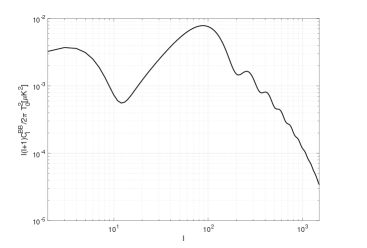
Figure 1: B-mode power spectrum due to inflation as well as for matter bounce.

where the function $f_{\mathbf{k}_{1}\mathbf{k}_{2}\mathbf{k}_{3}}^{s_{1}s_{2}s_{3}}$ can be written as

$$f_{\mathbf{k}_{1}\mathbf{k}_{2}\mathbf{k}_{3}}^{s_{1}s_{2}s_{3}}=\mathcal{G}\left(k_{1},k_{2},k_{3}\right)\times\left[\left(e_{im}^{s_{2}}e_{lj}^{s_{3}}-\frac{1}{2}e_{ml}^{s_{2}}e_{ij}^{s_{3}}\right)^{*}e_{ij}^{s_{1}*}k_{1m}k_{1l}+5\text{ Perms}\right].$$ (2.27)

The angular dependence comes with the polarization tensor $e_{ij}^{s_{i}}\equiv e_{ij}^{s_{i}}(\Omega_{\mathbf{k}_{i}})$ which is expressible in terms of spin $s$ weighted spherical harmonics. This quantity is calculated from the cubic order action given in Eq. (2.15). The form of the function $\mathcal{G}\left(k_{1},k_{2},k_{3}\right)$ in Eq. (2.27) depends upon the model being employed. In case of slow-roll inflation, $\mathcal{G}\left(k_{1},k_{2},k_{3}\right)$ is given in Ref. [34] whereas, in our case, for simple matter bounce, the expression is obtained in Ref. [19].

3 Bispectrum due to Matter Bounce

On account of the properties of Wigner 9j symbols in Eq. (2.25), that appear after performing angular integrations, it turns out that only for $\sum l_{i}=\text{odd}$, the B-mode auto-bispectrum in Eq. (2.24) is nonzero. Further, the bispectrum is nonzero only when all $l_{i}$’s are different.

In this work, we calculate bispectrum for $\sum l_{i}=33$. This implies 114 possibilities in total for the triple $\left(l_{1},l_{2},l_{3}\right)$. However, due to symmetry, we need to evaluate only one of the six permutations and rest others can be evaluated by noting the sign of permutation.

We obtain the analytical form of $B_{l_{1}l_{2}l_{3}}$ in Eq. (2.24) due to simple matter bounce after substituting the simplified form of the three point correlations of primordial perturbations from Eq. (B.1) in Eq. (2.25). Since we are considering only a specific regime (as per the discussions done in Appendix B) which contributes the most, we get the following approximate expression:

$$B_{l_{1}l_{2}l_{3}} \approx C\sum_{L_{i},l_{i}^{\prime}}\int_{0}^{\infty}x^{2}dx\left[\prod_{j=1}^{3}\int_{0}^{\infty}k_{j}^{2}dk_{j}T_{l_{j}}\left(k_{j}\right)j_{L_{j}}\left(xk_{j}\right)\right]\left[k_{1}^{2}\left(3\sqrt{3}\delta_{l_{1}^{\prime},2}-\delta_{l_{1}^{\prime},4}\right)\delta_{l_{2}^{\prime},2}\delta_{l_{3}^{\prime},2}+\text{ 2 perms}\right]$$

$$\times\left(i^{\sum L_{j}-l_{j}}\right)I_{L_{1},L_{2},L_{3}}^{0,0,0}I_{l_{1},L_{1},l_{1}^{\prime}}^{-2,0,2}I_{l_{2},L_{2},l_{2}^{\prime}}^{-2,0,2}I_{l_{3},L_{3},l_{3}^{\prime}}^{-2,0,2}\begin{Bmatrix}l_{1}^{\prime}&l_{2}^{\prime}&l_{3}^{\prime}\\ L_{1}&L_{2}&L_{3}\\ l_{1}&l_{2}&l_{3}\end{Bmatrix}\left[\frac{1}{\left(k_{1}k_{2}\right)^{3}}+\frac{1}{\left(k_{2}k_{3}\right)^{3}}+\frac{1}{\left(k_{3}k_{1}\right)^{3}}\right],$$ (3.1)

here the symbol $I_{L_{1}L_{2}L_{3}}^{s_{1}s_{2}s_{3}}$ in terms of Wigner 3j symbols is defined as

$$I_{L_{1}L_{2}L_{3}}^{s_{1}s_{2}s_{3}}=\sqrt{\frac{\prod_{i=1}^{3}\left(2L_{i}+1\right)}{4\pi}}\begin{pmatrix}L_{1}&L_{2}&L_{3}\\ s_{1}&s_{2}&s_{3}\end{pmatrix}.$$

The explicit expression of $C$ in Eq. (3.1) is given in Eq. (B.11). The simplification part of the three point function is discussed in Appendix B.

Presence of the Wigner symbols in the above expression assigns specific values to $L_{i}$’s for given $l_{i}$’s. For example, consider the Wigner 9j symbol.

$$\begin{Bmatrix}l_{1}^{\prime}&l_{2}^{\prime}&l_{3}^{\prime}\\ L_{1}&L_{2}&L_{3}\\ l_{1}&l_{2}&l_{3}\end{Bmatrix}.$$

This symbol can be written in terms of a sum over Wigner 3j symbols [35]. The Wigner symbols imply the following conditions

$$\left|l_{1}-l_{2}\right|\leq l_{3}\leq l_{1}+l_{2},\ \left|l_{i}-l_{i}^{\prime}\right|\leq L_{i}\leq l_{i}+l_{i}^{\prime}.$$ (3.2)

This means that we need to perform integrations over only certain combinations of $l$ and $L$. This turns out to be very helpful in devising numerical integration technique which is discussed in the next section. The results of numerical computation are given in section 5 where we do the comparison of the bispectrum between the two paradigms.

4 Numerical Computation of Bispectrum

In this section, we discuss the numerical techniques for the evaluation of the bispectra due to both inflation and the bounce. The details of the results, these techniques are based on, can be found in Appendix (A). The steps for calculating the bispectrum are as follows:

1. First of all, the values of $l_{i}$ and $L_{i}$’s are chosen such that they satisfy all the requirements of the Wigner 3j and 9j symbols present in Eq. (3.1). Thus for our case, in addition to the conditions in Eq. (3.2), we must also have $\sum L_{i}=\text{even}$ because of the presence of $I_{L_{1}L_{2}L_{3}}^{000}$.

2. As can be seen from Eq. (3.1) that we need to perform four integrations. One is over $x$ and other three are on $k_{i}$’s.

3. The procedure for integrating over $k$ variable was based on the presence/absence of the term $k_{t}=\sum k_{i}$ in the denominator. If it is absent, we will call bispectrum as separable and inseparable otherwise. Thus we take two cases

   • For separable form we evaluate the integral

     $$I_{x}\left(n,l,L\right)=\int k^{n}dkT_{l}\left(k\right)j_{L}\left(kx\right)$$ (4.1)

     for different values of $x$.

   • For an inseparable form, we first take Laplace’s transform and introduce another variable $y$ [20] and evaluate the following integral for different $x$ and $y$’s

     $$I_{x,y}\left(n,l,L\right)=\int k^{n}dkT_{l}\left(k\right)j_{L}\left(kx\right)e^{-ky}.$$ (4.2)

4. These integrals are then stored in an array for the relevant values of $n$, $l$ and $L$ for given $x$ (and $y$). We here emphasize that this integral evaluation part can easily be parallel implemented.

5. In order to retrieve integrals while doing integration over $x$ (and $y$) for different values of $n$, $l$ and $L$, we use the binary search method. We explain the method using an example later in this section. The method relies on two results derived in Appendix A.1.

6. We also need to compute Wigner 3j and 9j symbols. We did this computation using two methods which we also elaborate on later in this section.

7. The condition $\sum l_{i}=33$ along with Wigner 9j symbol gave 114 possibilities on the triple $(l_{1},l_{2},l_{3})$. The bispectrum will be same modulo a phase sign for different permutations of $(l_{1},l_{2},l_{3})$. This reduces the computation to 1/6.

All of the steps just discussed can be summarized in the flow chart shown in Figure 2 below.

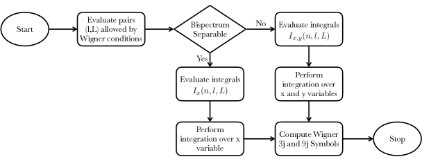
Figure 2: Flow chart of the algorithm for numerical calculation of the bispectrum. This very algorithm can be used for computing more complicated forms of bispectra.

4.1 Example of Binary Search Method

Next, we explain the $n$ tuple binary search method with an example. Suppose we have the following 3 tuple array

$$\{(1,1,3),(1,2,4),(1,3,-3),(2,0,5),(3,4,-2)\}.$$

Let us assume that we want to find out the location of the tuple $(3,4,-2)$. One obvious way would be to implement a linear search and to find locations of integers 3, 4 and $-2$, thereby finding the location of the tuple. A more efficient way would be to convert all of these tuples into an integer and search for just that integer using Theorem 1 of section (A.1). Also notice that the tuple array is in the lexicographic order in the sense described in Appendix A.

Now we apply Theorem 1 of section (A.1), according to which the base of representation would be $M\geq 9$. For $M=9$, the map would convert these tuples into the following

$$\{93,103,105,167,277\}.$$

Here we can see that the integers appear in ascending order as per Theorem 2 of section (A.1). After this, we can implement a binary search so that in place of searching the tuple $(3,4,-2)$, we just search the integer 277. This method can be used to store the integral $I_{x}(n,l,L)$ corresponding to say $(n,l,L)=(-2,1,3)$ and to later retrieve it while performing $x$ integration.

We must emphasize that the binary search method for tuples can be applied in all places where the location of a tuple is sought after storage. The method becomes more and more advantageous as the length of the tuple becomes larger and larger.

4.2 Wigner Symbols’ Computation

We now provide details about the Wigner 3j calculation. Since 9j symbols can be expressed in terms of 3j symbols, the discussion of 3j would suffice. We employed two methods of computation.

The first method is the Rasch Algorithm [36]. This is based on the Regge symmetries of the Wigner 3j symbols. The Rasch method employs 36 out of 72 symmetries. Thus by computing and storing one symbol, 36 other symbols are determined as well. This considerably reduces the computation time. For the evaluation of the symbols, we use fgsl which is a Fortran version of gsl. But it turned out that fgsl gives segmentation fault at larger values of l. So we use wigxjpf for the bispectrum evaluation at larger values of $l$ while calculating SNR.

Wigxjpf software [37] calculates these symbols using prime number factorization.

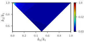
(a) Slow-roll Inflation

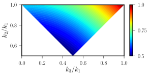
(b) Bounce

Figure 3: Comparison of the shape function normalized to unity.

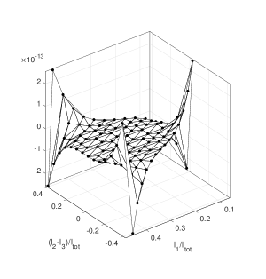
(a) Inflation

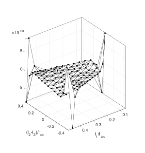
(b) Bounce

Figure 4: Comparison of the Bispectra plots for inflation and bounce cases. The bispectra values are obtained after taking tensor to scalar ratio $r=0.01$. In both cases, we have divided the bispectrum by the square of the tensor amplitude i.e., $\mathcal{P}_{T}^{2}$.

5 Results

In this section, we give all the results of our numerical computation. First of all, we compare the shape function or the non-gaussianity parameter $h_{\text{NL}}$ for inflation with that of matter bounce. This can be found in Figure 3. We see that the two bispectra are different for all three limits - squeezed, folded and equilateral.

The bispectra results for the two cases can be found in Figure 4. These plots have been generated by considering the tensor-to-scalar ratio $r=0.01$. We see that the peaks of the bispectrum in both cases appear at the permutations of $(l_{1},l_{2},l_{3})=(2,15,16)$. But the magnitude is very much different. In the case of inflation, the highest value of the bispectrum is found to be $\sim 6\times 10^{-11}$ while in bounce it is about $\sim 5\times 10^{-23}$. This feature is clearly different from the angular power spectrum where the values from both paradigms were the same. Thus the bispectrum is indeed able to distinguish between the two paradigms.

SNR is given by the following expression [20]

$$\sqrt{\sum_{l_{i}\leq l_{\text{max}}}\frac{B_{l_{1}l_{2}l_{3}}^{2}}{6C_{l_{1}}C_{l_{2}}C_{l_{3}}}}.$$ (5.1)

here $l_{\text{max}}$ is the value of maximum multipole $l$ used in the computation.

This expression for the SNR is valid for all triples $\left(l_{1},l_{2},l_{3}\right)$ which satisfy the conditions enforced by the Wigner 9j symbol, as was discussed above. The bispectrum for all permutations of say $\left(2,3,5\right)$ will be the same, apart from a phase factor. Thus the expression can be simplified by summing over only unique triples and thus can be written as

$$\sqrt{\sum_{l_{i}^{\text{unq}}\leq l_{\text{max}}}\frac{B_{l_{1}l_{2}l_{3}}^{2}}{C_{l_{1}}C_{l_{2}}C_{l_{3}}}},$$ (5.2)

where $l_{i}^{\text{unq}}$ depicts the fact that the sum is over unique triples. The SNR plot as a function of $l_{\text{max}}$ for tensor to scalar ratio $r\in\left\{0.1,0.01\right\}$ is shown in Figure 5. For $r=0.01$ and $l_{\text{max}}=100$, the SNR due to standard inflation turns out to be $\sim 10^{-5}$, whereas for bounce it is $\sim 10^{-18}$. Thus the SNR due to bounce is $\sim 10^{-13}$ times smaller than due to inflation, thereby making the signal due to bounce very difficult to detect. So a future detection of tensor mode bispectrum will be helpful in ruling out matter bounce model.

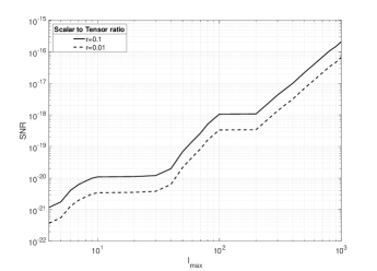
Figure 5: SNR for the bounce model for tensor-to-scalar ratio $r\in\{0.1,0.01\}$.

6 Conclusion

In this paper, we have analytically calculated the B-mode auto-bispectrum due to matter bounce. We also have computed the bispectrum numerically and compared it with that generated due to the standard inflationary paradigm. The numerical computation of bispectrum involves integration over 4 (or 5) integrals. Since the bispectrum $B_{l_{1}l_{2}l_{3}}$ exhibits symmetries in $(l_{1},l_{2},l_{3})$, the computation time can be reduced to 1/6. The bispectrum expression (3.1) contains summation over $L_{i}$’s which, in turn, are dependent upon $l_{i}$’s, as can be seen in Eq. (3.2). This gives us the advantage of evaluating $k$ integrals only for valid $(l,L)$ pairs, i.e., Eq. (4.1). This was followed by the $x$ integration. In order to avoid the repetitive calculation of same $k$ integrals, we saved the integral (4.1) information as a function of $x$ on an array. To serve this purpose, we developed a method for storing and retrieving data, using a binary search method for integer $n$ tuples. Two theorems provided by us ensure the certainty of the binary search method. For efficient evaluation, we first calculated the Wigner symbols by using the open source softwares, e.g., fgsl and wigxjpf. Then, we stored and retrieve the required symbols using the Rasch Algorithm. We think that the software wigxjpf used for the evaluation of Wigner symbols can be coupled with Rasch Algorithm to improve the computation speed.

The highest absolute value of B-mode bispectrum due to inflation, as per Fig. 4, is $\sim 6\times 10^{-11}$ which occurs at $(l_{1},l_{2},l_{3})=(2,15,16)$. We find that the B-mode auto-bispectrum due to matter bounce is about $10^{-12}$ times smaller as compared to this value and occurs at the same point. For numerical integration over $x$ (and $y$) variable(s), we checked that both the trapezoidal and rectangular integration methods were giving the same answer.

We also found that the shape functions for the two cases exhibit stark differences as can be seen in Fig. 3. We have also calculated the SNR in Figure 5. For its calculation, we use the same expression as used in Ref. [20]. The SNR for scalar-to-tensor ratio $r=0.01$ and $\l_{\text{max}}=100$ for inflation is $\sim 10^{-5}$. For matter bounce, this ratio is smaller by a factor of $\sim 10^{-13}$. This means that it would be even more difficult to detect signals due to bounce as compared to inflation. Thus a future detection of tensor bispectrum will rule out matter bounce model.

7 Acknowledgments

We are very much thankful to L. Sriramkumar of the Physics Department, IIT Madras. We are also indebted to Pankaj Jain of the Physics Department, IIT Kanpur for reading through the manuscript and suggesting valuable comments. We are very grateful to Rathul Nath Raveendran, Debika Choudhury for useful discussions. We wish to thank Indian Institute of Technology Madras, Chennai, India, for support through the Exploratory Research Project PHY/17-18/874/RFER/LSRI. RK is thankful to Pradeep Mishra of Mathematics Department, IIT Madras for vetting the mathematical appendix. RK also wishes to thank hospitality provided at IIT Kanpur where computing facilities supported by the Science and Engineering Research Board (SERB), Government of India were used. Further, we would also like to thank our anonymous referee for encouraging words and pointing one of the most important conclusions of our work that a future detection of tensor bispectrum will be helpful in ruling out matter bounce model. Finally, RK is very thankful to Prof. Roy Maartens for illuminating discussions.

Appendix A Numerical Strategies

In this appendix, we give details of the methods that underlie the numerical evaluation of the bispectrum form in Eq. (3.1). The evaluation hinges on two important results which we prove next.

A.1 A Binary Search Algorithm for Integer Tuples

For numerical evaluation of the integrals in Eq. (3.1), we stored integrals given in Eqs. (4.1) or (4.2) on an array, based on whether the bispectrum is separable or inseparable. The binary search algorithm plays a crucial role in the bispectrum determination for retrieving these integrals to perform integration over $x$ (and $y$) for different values of $l$, $L$ and $n$. It is known that the binary search is one of the fastest search method when the array is sorted.

Let $X$ denote the finite set of $n$ integers’ tuples, i.e.,

$$X=\left\{\left.\mathbf{x}^{j}\equiv\left(x_{1},x_{2},\ldots,x_{i}\right)\right|x_{i}\in\mathbb{Z},\ 1\leq j\leq N\right\}.$$

Further, let $\mathbf{x}\equiv\left(x_{1},x_{2},\ldots x_{n}\right)$ and $\mathbf{y}\equiv\left(y_{1},y_{2},\ldots,y_{n}\right)$ be two elements of $X$. We say $\mathbf{x}$ “comes before” $\mathbf{y}$ and write $\mathbf{x}\prec\mathbf{y}$ when either of these two cases are true

• $x_{1}<y_{1}$

• there exists an $i$ such that if $x_{j}=y_{j}$ for every $1\leq j<i$ then $x_{i}<y_{i}$.

Please notice that these are the conditions for dictionary ordering or lexicographic ordering, the same conditions due to which ‘car’ comes before ‘cat’. Thus according to our definition ‘car’ $\prec$ ‘cat’.

Let $\mathbf{x}^{1},\mathbf{x}^{2},\ldots\mathbf{x}^{k}$ be $k$ number of tuples of $X$, then these tuples are said to be dictionary ordered if there exists a permutation of indices $\left\{i_{1},i_{2},\ldots i_{n}\right\}$ such that $\mathbf{x}^{i_{1}}\prec\mathbf{x}^{i_{2}}\prec\ldots\prec\mathbf{x}^{i_{k}}$, where for $1\leq p\leq k$ we have $1\leq i_{p}\leq n$. Next is the notion of maximal element which would be defined as $m_{1}=\max\left\{x_{1}^{i_{k}},x_{2}^{i_{k}},\ldots,x_{n}^{i_{k}}\right\}$ and minimal element of $X$ would be defined as $m_{2}=\min\left\{x_{1}^{i_{1}},x_{2}^{i_{1}},\ldots,x_{n}^{i_{1}}\right\}$. In simple words, the maximal element is the largest integer of the tuple that comes last in the lexicographic ordering. Similarly, minimal is the smallest integer in the tuple that comes first. Notice that $m_{1}-m_{2}>0$, since if $m_{1}=m_{2}$ then there would only be one element in $X$.

As an example, consider the tuple set $X=\left\{\left(1,2,3\right),\left(-1,2,3\right),\left(1,2,5\right)\right\}$. The corresponding dictionary ordered set would be $\left\{\left(-1,2,3\right),\left(1,2,3\right),\left(1,2,5\right)\right\}$, maximal element $m_{1}$ would be $5$ and minimal element $m_{2}$ would be $-1$. The next result describes that there exists a one to one mapping between $n$ tuple set $X$ and $\mathbb{Z}$.

Theorem 1: Let $X$ be the finite set of $n$ tuples, then the function $f:X\to\mathbb{Z},\ f\left(\mathbf{a}\right)=\sum_{s=0}^{n-1}M^{s}a_{n-s}$ is one-one, where $M\geq m_{1}+\left|m_{2}\right|+1$.

Proof.

We will refer to $M$ as the base of representation. To show that the function $f$ is one-one, we demonstrate that

$$f\left(\mathbf{a}\right)=f\left(\mathbf{b}\right)\Rightarrow\mathbf{a}=\mathbf{b},$$

where $\mathbf{a}$, $\mathbf{b}\in X$. Now

$$f\left(\mathbf{a}\right)=f\left(\mathbf{b}\right)\Rightarrow\sum_{s=0}^{n-1}M^{s}\left(a_{n-s}-b_{n-s}\right)=0.$$

For convenience, let us denote $a_{p}-b_{p}=c_{p}$. Notice that $a\mod b$ gives the remainder when $a$ is divided by $b$ [38]. We perform the modular operation $n-1$ number of times with different powers of $M$, viz. $M^{n-1}$, $M^{n-2}$$\ldots,M$ to get the following equations

$$\begin{bmatrix}M^{n-1}&M^{n-2}&\ldots&M&1\\ 0&M^{n-2}&\ldots&M&1\\ \vdots&&&\vdots&\vdots\\ 0&0&\ldots&M&1\\ 0&0&\ldots&0&1\end{bmatrix}\begin{bmatrix}c_{1}\\ c_{2}\\ \vdots\\ c_{n-1}\\ c_{n}\end{bmatrix}=\begin{bmatrix}0\\ 0\\ \vdots\\ 0\\ 0\end{bmatrix}.$$

We notice that the matrix is upper triangular and the value of the determinant is $M^{n\left(n-1\right)/2}\neq 0$ if $M\neq 0$. Thus by the Cramer’s rule (see [39]), the given homogeneous system has only a trivial solution $\mathbf{c}=0$, thereby implying $\mathbf{a}=\mathbf{b}$. Therefore the given function is one-one. ∎

The result, we just proved shows that the function $f$ is one-one. If we restrict the range to $f\left(X\right)=D$, then the function $f:X\to D$ becomes bijective. We will call the function $f$ an “indexing scheme.” The next result shows that if a given tuple array is in the lexicographic order and the above indexing scheme is used, resulting array of integers is automatically sorted, i.e.,

$$\mathbf{x}^{i_{1}}\prec\mathbf{x}^{i_{2}}\prec\ldots\prec\mathbf{x}^{i_{k}}\Rightarrow f\left(\mathbf{x}^{i_{1}}\right)<f\left(\mathbf{x}^{i_{2}}\right)<\ldots<f\left(\mathbf{x}^{i_{k}}\right).$$ (A.1)

This means that one need not use any sorting methods and hence one can directly use the binary search method. The proof follows next.

Theorem 2: Let $\mathbf{a}$ and $\mathbf{b}$ be two $n$ tuples of $X$ then $\mathbf{a}\succ\mathbf{b}\Rightarrow f\left(\mathbf{a}\right)>f\left(\mathbf{b}\right)$.

Proof.

As per the definition of ‘$\succ$’, we need to consider two cases for $\mathbf{a}\succ\mathbf{b}$:

• $b_{1}<a_{1}$

• there exists an $i$ such that if $a_{j}=b_{j}$ for every $1\leq j<i$ then $b_{i}<a_{i}$.

Let us analyze Case 1 first. We calculate the quantity $f\left(\mathbf{a}\right)-f\left(\mathbf{b}\right)$ which is equal to

$$\sum_{s=0}^{n-1}M^{s}\left(a_{n-s}-b_{n-s}\right)=M^{n-1}\left(a_{1}-b_{1}\right)+\sum_{s=0}^{n-2}M^{s}\left(a_{n-s}-b_{n-s}\right).$$ (A.2)

But $a_{i}$ and $b_{i}$ are integers therefore $a_{1}>b_{1}\Rightarrow a_{1}-b_{1}\geq 1$ and since $m_{1}$ and $m_{2}$ are the maximal and minimal elements of $X$ therefore $m_{2}-m_{1}\leq a_{i}-b_{i}$ for every $1\leq i\leq n$. Thus we must have

$$M^{n-1}+\left(m_{2}-m_{1}\right)\left(\frac{M^{n-1}-1}{M-1}\right)\leq f\left(\mathbf{a}\right)-f\left(\mathbf{b}\right).$$

The second term is obtained by summing over a geometric series. For further analysis, notice that $M\geq m_{1}+\left|m_{2}\right|+1\geq m_{1}-m_{2}+1$ so that

$$\frac{m_{2}-m_{1}}{M-1}\geq-1\Rightarrow\left(\frac{m_{2}-m_{1}}{M-1}\right)\left(M^{n-1}-1\right)\geq-\left(M^{n-1}-1\right).$$ (A.3)

So we have

$$M^{n-1}-\left(M^{n-1}-1\right)\leq M^{n-1}+\left(m_{2}-m_{1}\right)\left(\frac{M^{n-1}-1}{M-1}\right)\leq f\left(\mathbf{a}\right)-f\left(\mathbf{b}\right).$$ (A.4)

From this, we get the required inequality $f\left(\mathbf{a}\right)>f\left(\mathbf{b}\right)$. Now let us consider the second Case. In this case, we can write $f\left(\mathbf{a}\right)-f\left(\mathbf{b}\right)$ as

$$\sum_{s=0}^{n-1}M^{s}\left(a_{n-s}-b_{n-s}\right)=M^{n-i}\left(a_{i}-b_{i}\right)+\sum_{s=n-i+1}^{n-1}M^{s}\left(a_{n-s}-b_{n-s}\right).$$ (A.5)

This follows since $a_{j}=b_{j}$ when $1\leq j<i$. Using the similar reasoning as was done for Case 1 we get

$$M^{n-i}-\left(M^{n-i}-1\right)\leq M^{n-i}+\left(m_{2}-m_{1}\right)\frac{M^{n-i}-1}{M-1}\leq f\left(\mathbf{a}\right)-f\left(\mathbf{b}\right).$$ (A.6)

Thus again the inequality $f\left(\mathbf{a}\right)>f\left(\mathbf{b}\right)$ is satisfied. ∎

Appendix B Simplification of Bispectrum due to Matter Bounce

The function $\mathcal{G}\left(k_{1},k_{2},k_{3}\right)$ appearing in Eq. (2.27) for matter bounce can be written as [21]

$$\mathcal{G}\left(k_{1},k_{2},k_{3}\right)=\left(2\pi\right)^{-17/2}\,8M_{\text{Pl}}^{2}\left(\mathbb{G}\left(k_{1},k_{2},k_{3}\right)+\text{c.c.}\right),$$ (B.1)

where $M_{\text{Pl}}=10^{56}\,{\rm Mpc}^{-1}$ represents the Planck mass expressed in the Mpc units, ‘c.c.’ represents the complex conjugation of the quantity coming before it. In Ref. [21], in order to evaluate the tensor bispectra, authors divided the time regime into three domains and showed that, only in the third domain, it contributes the most. In that domain, $\mathbb{G}(k_{1},k_{2},k_{3})$ takes the following form

$$\mathbb{G}\left(k_{1},k_{2},k_{3}\right) = \left[A_{k_{1}}^{*}A_{k_{2}}^{*}A_{k_{3}}^{*}J_{0}\left(\beta\right)+\text{Perm}\left(A_{k_{1}}^{*}A_{k_{2}}^{*}B_{k_{3}}^{*}\right)J_{1}\left(\beta\right)+\text{Perm}\left(A_{k_{1}}^{*}B_{k_{2}}^{*}B_{k_{3}}^{*}\right)J_{2}\left(\beta\right)+\right.$$ (B.2)

$$\left.\qquad\qquad\qquad\qquad\qquad\qquad B_{k_{1}}^{*}B_{k_{2}}^{*}B_{k_{3}}^{*}J_{3}\left(\beta\right)\right]\times\left(-\frac{ia_{0}}{4k_{0}}\right)h_{k_{1}}h_{k_{2}}h_{k_{3}}.$$

In this equation, $a_{0}=10^{-30}$ is the minimum value of the scale factor that the Universe takes at the bounce, $k_{0}^{-1}=10^{-20}{\rm Mpc}$ is the energy scale that determines the duration of bounce. Other quantities are defined in the following manner:

$$h_{k}=A_{k}+B_{k}f\left(\eta\right),\ f\left(x\right)=\frac{x}{1+x^{2}}+\tan^{-1}\left(x\right),$$ (B.3)

with

$$B_{k} = \frac{\left(1+\alpha^{2}\right)^{2}}{2a_{0}\alpha^{2}M_{\text{pl}}\sqrt{k}}\left[\frac{3ik_{0}}{\alpha^{2}k}+\frac{3}{\alpha}-\frac{ik}{k_{0}}\right]\exp\left(\frac{i\alpha k}{k_{0}}\right),\quad$$ (B.4)

$$A_{k} = \frac{1}{a_{0}\alpha^{2}M_{\text{pl}}\sqrt{k}}\left(1+\frac{ik_{0}}{\alpha k}\right)\exp\left(\frac{i\alpha k}{k_{0}}\right)+f\left(\alpha\right)B_{k},$$ (B.5)

In Eq. (B.3), $\eta$ is the comoving time at which the calculation is performed. The constant $\alpha=10^{5}$ is chosen so that the relevant comoving length scales $k\ll k_{0}/\alpha$ and that the tensor power spectrum becomes scale invariant. The constants $J_{i}\left(\beta\right)$ are defined through an integral

$$J_{n}\left(x\right)=\int_{0}^{x}\left(1+y^{2}\right)^{2}f^{n}\left(y\right),$$

function $f\left(y\right)$ being given in Eq. (B.3). The symbol $\text{Perm}\left(A_{k_{1}}B_{k_{2}}C_{k_{3}}\right)$ denotes all possible permutations of the terms inside the bracket with the given subscripts. For example

$$\text{Perm}\left(A_{k_{1}}A_{k_{2}}B_{k_{3}}\right)=A_{k_{1}}A_{k_{3}}B_{k_{2}}+A_{k_{1}}A_{k_{3}}B_{k_{1}}+A_{k_{1}}A_{k_{2}}B_{k_{3}}.$$

Simplification of the term inside parenthesis of Eq. (B.1) becomes the following:

$$\mathbb{G}+\mathbb{G}^{*} =\left[\left(cJ_{0}-J_{1}\right)\text{Perm}\left(\Lambda_{\lambda_{1}}\phi_{\lambda_{2}}\Lambda_{\lambda_{3}}\right)+\left(c^{2}J_{0}-J_{2}\right)\text{Perm}\left(\theta_{\lambda_{1}}\Lambda_{\lambda_{2}}\phi_{\lambda_{3}}\right)+\left(c^{3}J_{1}-cJ_{3}\right)\text{Perm}\left(\theta_{\lambda_{1}}\Gamma_{\lambda_{2}}\phi_{\lambda_{3}}\right)\right.$$

$$+\left(c^{2}J_{1}-cJ_{2}\right)\text{Perm}\left(\Lambda_{\lambda_{1}}\Gamma_{\lambda_{2}}\phi_{\lambda_{3}}\right)+\left(c^{2}J_{1}-cJ_{2}+c^{3}J_{0}-J_{3}\right)\text{Perm}\left(\theta_{\lambda_{1}}\theta_{\lambda_{2}}\phi_{\lambda_{3}}\right)$$

$$\left.+\left(3c^{2}J_{1}-3cJ_{2}-c^{3}J_{0}+J_{3}\right)\phi_{1}\phi_{2}\phi_{3}+\left(c^{3}J_{2}-c^{2}J_{3}\right)\text{Perm}\left(\Gamma_{\lambda_{1}}\Gamma_{\lambda_{2}}\phi_{\lambda_{3}}\right)\right],$$ (B.6)

where the functions are defined below.

$$\Lambda = \left|A\right|^{2}=\frac{1}{(2k_{0}M_{\text{pl}}^{4}a_{0}^{5})^{1/3}k\alpha^{4}}\left[\left(1+\frac{3f\left(\alpha\right)\left(1+\alpha^{2}\right)^{2}}{2\alpha}\right)^{2}+\left\{\frac{k_{0}}{\alpha k}+\frac{f\left(\alpha\right)\left(1+\alpha^{2}\right)^{2}}{2}\left(\frac{3k_{0}}{\alpha^{2}k}-\frac{k}{k_{0}}\right)\right\}^{2}\right],$$

$$\Gamma = \left|B\right|^{2}=\frac{\left(\alpha^{-1}+\alpha\right)^{4}}{(M_{\text{pl}}^{4}k_{0}2^{7}a_{0}^{5})^{1/3}k}\left[\frac{9}{\alpha^{2}}+\left(\frac{3k_{0}}{\alpha^{2}k}-\frac{k}{k_{0}}\right)^{2}\right],$$

$$\phi = {\rm Re}\left(AB^{*}\right)=\frac{\left(1+\alpha^{2}\right)^{2}}{(2^{4}k_{0}^{4}M_{\text{pl}}^{4}a_{0}^{5})^{1/3}\alpha^{4}},$$

$$\theta = {\rm Im}\left(AB^{*}\right)=\frac{\left(1+\alpha^{2}\right)^{2}}{(M_{\text{pl}}^{4}k_{0}a_{0}^{5}2^{4})^{1/3}k\alpha^{4}}\left[\frac{2}{\alpha}+\frac{3k_{0}^{2}}{\alpha^{3}k^{2}}+\frac{f\left(\alpha\right)\left(1+\alpha^{2}\right)^{2}}{2}\left\{\left(\frac{3k_{0}}{\alpha^{2}k}-\frac{k}{k_{0}}\right)^{2}+\frac{9}{\alpha^{2}}\right\}\right].$$

These functions can be further simplified, owing to the values of the various parameters of the theory and the following final form is obtained

$$\Lambda\approx\frac{9\pi^{2}C_{1}}{2^{1/3}k^{3}},\quad\Gamma\approx\frac{9C_{1}}{2^{7/3}k^{3}},\quad\theta\approx\frac{9C_{1}}{2^{7/3}k^{3}},\quad\phi\approx\frac{C_{2}}{2^{4/3}},$$ (B.7)

The constants $C_{1},C_{2}$ appearing in Eqs. (B.7) are:

$$C_{1} = \left(\frac{k_{0}^{5}}{M_{\text{pl}}^{4}a_{0}^{5}}\right)^{1/3}=\left(10^{26}{\rm Mpc}^{-1}\right)^{1/3},$$ (B.8)

$$C_{2} = \left(\frac{1}{M_{\text{pl}}^{4}a_{0}^{5}k_{0}^{4}}\right)^{1/3}=\left(10^{-154}{\rm Mpc}^{-8}\right)^{1/3}.$$ (B.9)

Since $C_{2}$ appears with $\phi$ term, this means that the $\phi\phi$ and other higher order terms will be suppressed, due to which, the function $\mathbb{G}$ of Eq. B.6 can finally be written as

$$\mathbb{G}=C\left[\frac{1}{\left(k_{1}k_{2}\right)^{3}}+\frac{1}{\left(k_{2}k_{3}\right)^{3}}+\frac{1}{\left(k_{3}k_{1}\right)^{3}}\right],$$ (B.10)

the constant $C$ being

$$C = \frac{72\times 10^{-34}}{\pi^{6}5\sqrt{7}}[8\pi^{2}\left\{2\pi^{2}\left(cJ_{0}-J_{1}\right)+c^{2}J_{0}+c^{2}J_{1}-J_{2}\left(c+1\right)\right\}$$ (B.11)

$$+\left(2c^{3}+c^{2}\right)J_{1}+c^{3}J_{0}+J_{2}\left(c^{3}-c\right)-J_{3}\left(1+2c+c^{3}\right)],$$

and $c=f\left(\beta\right)$.

References

- [1] V. F. Mukhanov, H. Feldman, and R. H. Brandenberger, Theory of cosmological perturbations. Part 1. Classical perturbations. Part 2. Quantum theory of perturbations. Part 3. Extensions, Phys.Rept. 215 (1992) 203–333.
- [2] B. A. Bassett, S. Tsujikawa, and D. Wands, Inflation dynamics and reheating, Rev. Mod. Phys. 78 (2006) 537–589, [astro-ph/0507632].
- [3] L. Sriramkumar, An introduction to inflation and cosmological perturbation theory, arXiv:0904.4584.
- [4] D. Baumann, Inflation, in Physics of the large and the small, TASI 09, proceedings of the Theoretical Advanced Study Institute in Elementary Particle Physics, Boulder, Colorado, USA, 1-26 June 2009, pp. 523–686, 2011. arXiv:0907.5424.
- [5] A. Linde, Inflationary Cosmology after Planck 2013, in Proceedings, 100th Les Houches Summer School: Post-Planck Cosmology: Les Houches, France, July 8 - August 2, 2013, pp. 231–316, 2015. arXiv:1402.0526.
- [6] J. Martin, C. Ringeval, and R. Trotta, Hunting Down the Best Model of Inflation with Bayesian Evidence, Phys. Rev. D83 (2011) 063524, [arXiv:1009.4157].
- [7] J. Martin, C. Ringeval, and V. Vennin, Encyclopedia Inflationaris, Phys. Dark Univ. 5-6 (2014) 75–235, [arXiv:1303.3787].
- [8] J. Martin, C. Ringeval, R. Trotta, and V. Vennin, The Best Inflationary Models After Planck, JCAP 1403 (2014) 039, [arXiv:1312.3529].
- [9] J. Martin, C. Ringeval, and V. Vennin, How Well Can Future CMB Missions Constrain Cosmic Inflation?, JCAP 1410 (2014), no. 10 038, [arXiv:1407.4034].
- [10] G. Gubitosi, M. Lagos, J. Magueijo, and R. Allison, Bayesian evidence and predictivity of the inflationary paradigm, JCAP 1606 (2016), no. 06 002, [arXiv:1506.0914].
- [11] M. Novello and S. E. P. Bergliaffa, Bouncing Cosmologies, Phys. Rept. 463 (2008) 127–213, [arXiv:0802.1634].
- [12] Y.-F. Cai, Exploring Bouncing Cosmologies with Cosmological Surveys, Sci. China Phys. Mech. Astron. 57 (2014) 1414–1430, [arXiv:1405.1369].
- [13] D. Battefeld and P. Peter, A Critical Review of Classical Bouncing Cosmologies, Phys. Rept. 571 (2015) 1–66, [arXiv:1406.2790].
- [14] M. Lilley and P. Peter, Bouncing alternatives to inflation, Comptes Rendus Physique 16 (2015) 1038–1047, [arXiv:1503.0657].
- [15] A. Ijjas and P. J. Steinhardt, Implications of Planck2015 for inflationary, ekpyrotic and anamorphic bouncing cosmologies, Class. Quant. Grav. 33 (2016), no. 4 044001, [arXiv:1512.0901].
- [16] R. Brandenberger and P. Peter, Bouncing Cosmologies: Progress and Problems, Found. Phys. 47 (2017), no. 6 797–850, [arXiv:1603.0583].
- [17] A. A. Starobinsky, Spectrum of relict gravitational radiation and the early state of the universe, JETP Lett. 30 (1979) 682–685.
- [18] F. Finelli and R. Brandenberger, On the generation of a scale invariant spectrum of adiabatic fluctuations in cosmological models with a contracting phase, Phys. Rev. D65 (2002) 103522, [hep-th/0112249].
- [19] R. N. Raveendran, D. Chowdhury, and L. Sriramkumar, Viable tensor-to-scalar ratio in a symmetric matter bounce, JCAP 1801 (2018), no. 01 030, [arXiv:1703.1006].
- [20] H. W. H. Tahara and J. Yokoyama, CMB B-mode auto-bispectrum produced by primordial gravitational waves, PTEP 2018 (2018), no. 1 013E03, [arXiv:1704.0890].
- [21] D. Chowdhury, V. Sreenath, and L. Sriramkumar, The tensor bi-spectrum in a matter bounce, JCAP 1511 (2015) 002, [arXiv:1506.0647].
- [22] Planck Collaboration, N. Aghanim et. al., Planck 2018 results. VI. Cosmological parameters, arXiv:1807.0620.
- [23] M. Zaldarriaga and U. Seljak, An all sky analysis of polarization in the microwave background, Phys. Rev. D55 (1997) 1830–1840, [astro-ph/9609170].
- [24] J. N. Goldberg, A. J. MacFarlane, E. T. Newman, F. Rohrlich, and E. C. G. Sudarshan, Spin s spherical harmonics and edth, J. Math. Phys. 8 (1967) 2155.
- [25] E. T. Newman and R. Penrose, Note on the Bondi-Metzner-Sachs group, J. Math. Phys. 7 (1966) 863–870.
- [26] T. Dray, The relationship between monopole harmonics and spin-weighted spherical harmonics, Journal of Mathematical Physics 26 (1985), no. 5 1030–1033, [https://doi.org/10.1063/1.526533].
- [27] T. Dray, A unified treatment of wigner d functions, spin-weighted spherical harmonics, and monopole harmonics, Journal of Mathematical Physics 27 (1986), no. 3 781–792, [https://doi.org/10.1063/1.527183].
- [28] M. Shiraishi, Probing the Early Universe with the CMB Scalar, Vector and Tensor Bispectrum. PhD thesis, Nagoya U., 2012-03. arXiv:1210.2518.
- [29] G. W. Horndeski, Second-order scalar-tensor field equations in a four-dimensional space, International Journal of Theoretical Physics 10 (1974), no. 6 363–384.
- [30] C. Deffayet, G. Esposito-Farese, and A. Vikman, Covariant Galileon, Phys.Rev. D79 (2009) 084003, [arXiv:0901.1314].
- [31] C. Deffayet, S. Deser, and G. Esposito-Farese, Arbitrary -form Galileons, Phys. Rev. D82 (2010) 061501, [arXiv:1007.5278].
- [32] C. Deffayet, O. Pujolas, I. Sawicki, and A. Vikman, Imperfect Dark Energy from Kinetic Gravity Braiding, JCAP 1010 (2010) 026, [arXiv:1008.0048].
- [33] M. Ostrogradsky, Memoires sur les equations differentielles relatives au probleme des isoperimetres, Mem. Ac. St. Petersbourg VI (1850) 385.
- [34] X. Gao, T. Kobayashi, M. Yamaguchi, and J. Yokoyama, Primordial non-Gaussianities of gravitational waves in the most general single-field inflation model, Phys. Rev. Lett. 107 (2011) 211301, [arXiv:1108.3513].
- [35] V. Khersonskii, A. Moskalev, and D. Varshalovich, Quantum Theory Of Angular Momemtum. World Scientific Publishing Company, 1988.
- [36] J. Rasch and A. C. H. Yu, Efficient storage scheme for precalculated wigner 3j, 6j and gaunt coefficients, SIAM Journal on Scientific Computing 25 (2004), no. 4 1416–1428, [https://doi.org/10.1137/S1064827503422932].
- [37] H. Johansson and C. Forssén, Fast and accurate evaluation of wigner 3, 6, and 9 symbols using prime factorization and multiword integer arithmetic, SIAM Journal on Scientific Computing 38 (2016), no. 1 A376–A384, [https://doi.org/10.1137/15M1021908].
- [38] J. Gallian, Contemporary Abstract Algebra. Cengage Learning, 2016.
- [39] K. Hoffman and R. Kunze, Linear Algebra. Prentice-Hall Mathematics Series. N.J., Prentice-Hall, 1971.