The quantum algorithm for graph isomorphism problem

Abstract

The graph isomorphism (GI) problem is the computational problem of finding a permutation of vertices of a given graph $G_{1}$ that transforms $G_{1}$ to another given graph $G_{2}$ and preserves the adjacency. In this work, we propose a quantum algorithm to determine whether there exists such a permutation. To find such a permutation, we introduce isomorphic equivalent graphs of the given graphs to be tested. We proof that the GI problem of the equivalent graphs is equivalent to the GI problem of the given graphs. The idea of the algorithm is to determine whether there exists a permutation can transform the eigenvectors of the adjacency matrix of the equivalent graphs each other. The cost time of the algorithm is polynomial.

I Introduction

The GI problem has been heavily studied in computer scienceKobler et al. (2012). Although GI problem for many special classes of graphs can be solved in polynomial time, and in practice graph isomorphism can often be solved efficientlyMcKay et al. (1981), the universal polynomial for GI is still open. The problem is not known to be solvable in polynomial time nor to be NP-complete, and therefore may be in the computational complexity class NP-intermediate. On the 11th of December 2015, L´aszl´o Babai proposed a quasi-polynomial algorithm on classical computer for GI problem other than Johnson graphsBabai (2016). The GI problem is believed to be of comparable computational difficulty as well as integer factorization problemArora and Barak (2009). However, the integer factorization problem can be settled by Shor’s algorithm in polynomial time, but the efficient quantum algorithm for GI is not known.

A number of researchers have considered the quantum physics-based algorithms for solving the graph isomorphism problem. In some of these algorithms, quantum systems droved by the Hamiltonians defined by the topology structure of the GI instance are settledRudolph (2002); Shiau (2005); Gamble et al. (2010); Shiau et al. (2003). Evolution results of the quantum system droved by different Hamiltonians imply that whether the two graphs are isomorphic. In the algorithms based on the continuous time quantum walk on graphs, the adjacency matrix of the associated graph is used to define the Hamiltonian $H(G)$ that drive the system. The state of system is changed by the unitary operator $U\left(G\right)={e^{-iH\left(G\right)t}}$. For the same initial state and the same sample time, if the measurement values of the systems droved by distinct Hamiltonians are equal, then the algorithm judges that the two graphs are isomorphic. The GI test algorithms based on discrete quantum are similarBerry and Wang (2011). However, both the continuous time quantum and the discrete time quantum walk on graphs are invalid for distinguishing the pairs of non-isomorphic strongly regular graphs with the same parameters even increasing the number of walkers or adding interacting between walkersSmith (2010); Berry and Wang (2011).

Another kind of quantum algorithm for solving the GI problem are based the adiabatic quantum evolution. In these algorithms, every permutation in the symmetry group $S_{n}$ is encoded as a binary vector which corresponds a computational basis stateGaitan and Clark (2014); Hen and Young (2012); Tamascelli and Zanetti (2014). Defining a time depended Hamiltonian $H(t)$. the $H(0)$ is a proper initial Hamiltonian whose ground state is easily preparing and the $H(T)$ is ending Hamiltonian whose ground state is a valid permutation for GI problem. Via adiabatic quantum evolution $T$ time, if the quantum system ending at a ground state corresponds a permutation, then the given graphs are isomorphic. These algorithms can distinguish non-isomorphism SRG with the same parameters. However, finding the time complexity of the algorithms is intricate since obtaining the energy gap of Hamiltonians is an open problem and the number of permutations needs to encode is $N!$ which is too large.

In our scheme, the permutation is not directly checked one by one. We introduce a kind of graphs correspond the original given graphs, the GI problem of such kind of graphs is equivalent to the GI problem of the given graphs, hence we call it isomorphic equivalent graph. The lowest eigenvalue of the Hamiltonian defined by the adjacency matrix of isomorphic equivalent graph is simple, namely the ground state is a non-degenerate state. After we prepare the ground states of distinct Hamiltonians, we check that whether these ground states can transfer to each other by a permutation matrix. If yes, then the two original given graphs are isomorphic, otherwise they are non-isomorphic. We introduce an he altered Grover algorithm, and acquire such a matrix by this algorithm. Since quantum algorithm for the GI problem of pairs of SRGs with the same parameters are hard, we illustrate our algorithm via the instances of SRGs.

This paper is organized as follows: the second section presents isomorphic conditions of isomorphic equivalent graphs. In the third section, the procedure of ground state of the equivalent graphs of SRG preparing is given. The fourth section discusses how to determine the transfer matrix between the ground states. The time complexity be presented in the fifth section, and the final section provides conclusions.

II Equivalent graph of isomorphism

A graph, denoted as $G(V,E)$, consists of a vertex set $V$ and an edge set $E$. The set $E$ is a subset of $V\times V$, which implies the connection relationship between pairs of vertices in $V$. The connection relationship of $G$ is generally represented via the adjacency matrix $A$. It is a $N\times N$ real symmetric matrix, where $A_{jk}=1$ if vertex $v_{j}$ and $v_{k}$ are connected otherwise $A_{jk}=0$. For graphs with loops, the diagonal entry is the number of loop attached on that vertex and the degree is the sum of the number of neighbors and the diagonal entry. For loop-less graphs, the diagonal entry $A_{jj}$=0 and the number of neighbors of a vertex is known as its degree.

For two given loop-less graphs $G_{1}$ and $G_{2}$, it is well known that $G_{1}$ is isomorphic to $G_{2}$ if and only if there exist a permutation matrix $P$ such that ${A_{2}}=P{A_{1}}{P^{T}}$ , where $A_{1}$ and $A_{2}$ are the adjacency matrices of $G_{1}$ and $G_{2}$ respectly. Now considering add a loop to every vertex of $G_{1}$ and $G_{2}$, the result graphs be denoted as $\widetilde{G_{1}}$ and $\widetilde{G_{2}}$. The correspond adjacency matrices are $A_{1}^{\prime}{\rm{=}}{A_{1}}{\rm{+}}I$ and $A_{2}^{\prime}{\rm{=}}{A_{2}}{\rm{+}}I$. Adding the equal number of loops to every vertex does not change the adjacency of the original graph. Hence the isomorphism between $\widetilde{G_{1}}$ and $\widetilde{G_{2}}$ is equivalent to the isomorphism between $G_{1}$ and $G_{2}$. The isomorphism of $\widetilde{G_{1}}$ and $\widetilde{G_{2}}$ apparently be implied in the below theorem.

Theorem 1.

Graphs $\widetilde{G_{1}}$ and $\widetilde{G_{2}}$are isomorphic if and only if there exists a permutation matrix $P$, such that equation $A_{2}^{\prime}=P{A_{1}^{\prime}}{P^{T}}$ satisfies.

More operations can be executed on graph $\widetilde{G_{1}}$ and $\widetilde{G_{2}}$ such that the isomorphism between the resulting graphs imply the isomorphism between the original given graph $G_{1}$ and $G_{2}$. Now, choosing a pair vertices $v\in V(\widetilde{G_{1}})$ and $w\in V({\widetilde{G_{2}}})$, deleting the loop of $v$ and $w$ in $\widetilde{G_{1}}$ and $\widetilde{G_{2}}$. The resulting spanning subgraph are denoted as $\widetilde{G_{1}^{v}}$ and $\widetilde{G_{2}^{w}}$ respectively. A similar theorem can be obtained.

Theorem 2.

Graphs $\widetilde{G_{1}}$ and $\widetilde{G_{2}}$ are isomorphic if and only if there exist a pair of vertices $v$ and $w$ such that $\widetilde{G_{1}^{v}}$ and $\widetilde{G_{2}^{w}}$ are isomorphism.

If $\widetilde{G_{1}}$ and $\widetilde{G_{2}}$ are isomorphic, then there exist a isomorphic mapping $f$ and a pair of vertices $v$ and $w$ such that $f$ maps $v$ to $w$,namely

$$f:v\to w$$

. Deleting the loop of $v$ and $w$ in$\widetilde{G_{1}}$ and $\widetilde{G_{2}}$ to obtain the spanning subgraph $\widetilde{G_{1}^{v}}$ and $\widetilde{G_{2}^{w}}$. Apprently, the map $f$ is aslo a isomorphic map from $\widetilde{G_{1}^{v}}$ to $\widetilde{G_{2}^{w}}$.

Analogously, if graphs $\widetilde{G_{1}^{v}}$ and $\widetilde{G_{2}^{w}}$ are isomorphic, then there exists a isomorphic map $f$ such that $f:v\to w$. Adding a loop to $v$ and $w$, one will obtain graphs $\widetilde{G_{1}}$ and $\widetilde{G_{2}}$. Then the map $f$ is an isomorphic mapping from $\widetilde{G_{2}^{w}}$ to $\widetilde{G_{2}^{w}}$.

Theorem 3.

$\widetilde{G_{1}^{v}}$ and $\widetilde{G_{2}^{w}}$ are isomorphic if and only if there exists a permutation matrix $Q$ such that $A_{2}^{w}=QA_{1}^{v}{Q^{T}}$, where $A_{1}^{v}$ and $A_{2}^{w}$ are adjacency matrices of $\widetilde{G_{2}^{w}}$ and $\widetilde{G_{2}^{w}}$ respectively.

By proper relabeling, one can give vertices $v$ and $w$ index $1$, then

$$A_{2}^{w}=A_{2}^{\prime}-\left[{\begin{array}[]{*{20}{c}}1&0&\ldots&0\\ 0&0&{}\hfil&{}\hfil\\ \vdots&{}\hfil&{}\hfil&{}\hfil\\ 0&{}\hfil&{}\hfil&0\end{array}}\right],$$

and

$$A_{1}^{v}=A_{1}^{\prime}-\left[{\begin{array}[]{*{20}{c}}1&0&\ldots&0\\ 0&0&{}\hfil&{}\hfil\\ \vdots&{}\hfil&{}\hfil&{}\hfil\\ 0&{}\hfil&{}\hfil&0\end{array}}\right].$$

Based on theorem 2, $\widetilde{G_{1}^{v}}$ and $\widetilde{G_{2}^{w}}$ are isomorphic then $\widetilde{G_{1}}$ and $\widetilde{G_{2}}$ are isomorphic. Hence, there exists a permutation matrix Q such that $A_{2}^{\prime}=QA_{1}^{\prime}{Q^{T}}$. this leads to

$$A_{2}^{\prime}-\left[{\begin{array}[]{*{20}{c}}1&0&\ldots&0\\ 0&0&{}\hfil&{}\hfil\\ \vdots&{}\hfil&{}\hfil&{}\hfil\\ 0&{}\hfil&{}\hfil&0\end{array}}\right]=QA_{1}^{\prime}{Q^{T}}-Q\left[{\begin{array}[]{*{20}{c}}1&0&\ldots&0\\ 0&0&{}\hfil&{}\hfil\\ \vdots&{}\hfil&{}\hfil&{}\hfil\\ 0&{}\hfil&{}\hfil&0\end{array}}\right]{Q^{T}}.$$ (1)

Analogously, if the $A_{2}^{w}=QA_{1}^{v}{Q^{T}}$ valid, then $\widetilde{G_{1}}$ and $\widetilde{G_{2}}$ are isomorphic. by Theorem 2, $\widetilde{G_{1}^{v}}$ and $\widetilde{G_{2}^{w}}$ are isomorphic.

Theorem 4.

Loop-less graphs $G_{1}$ and $G_{2}$ are isomorphic if and only if there exist a pair of vertices $v$ and $w$ such that $\widetilde{G_{1}^{v}}$ and $\widetilde{G_{2}^{w}}$ are isomorphism.

From the above theorems, the isomorphism problem between $G_{1}$ and $G_{2}$ can be reduced to the isomorphism problem between $\widetilde{G_{1}^{v}}$ and $\widetilde{G_{2}^{w}}$. Hence, we call the graph $\widetilde{G_{1}^{v}}$ and $\widetilde{G_{2}^{w}}$ the isomorphic equivalent graphs of $G_{1}$ and $G_{2}$ respectively. In next sections, we will see that finding isomorphic permutation matrix between equivalent graphs is more facile than the original given graphs. We give an instance in Fig.(1)

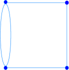
(a) A loop-less graph

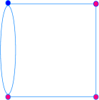
(b) One of configuration by adding three loops

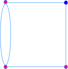
(c) Another configuration by adding three loops

Figure 1: Diffirent configurations of a given graph by adding loops. The red vertices are attached to a loop and the blue are not. There is only one blue vertex in both of the two graphs. For isomorphic graphs, there exists one pair of vertices without loops such that the isomorphic graphs are isomorphic. For non-isomorphic graph, one cann’t find such a pair of vertices in the two graphs respectively.

III The spectrum of isomorphic equivalent SRG

Since distinguishing non-isomorphic SRGs is hard by quantum algorithm, we will apply the algorithm to the GI problem of SRG at first. First of all, we will introduce the spectrum of equivalent SRG which is significant for the preparing a non-degenerate eigenvector. The connection relationship of a SRG satisfiesCvetković et al. (1980)

(i). It is neither a complete graph nor an empty graph,

(ii). Any two adjacent vertices have $a$ common adjacent vertices

(iii). Any two non-adjacent vertices have $c$ common adjacent vertices

If the number and degree of the SRG are $N$ and $k$ respectively, then it is labelled SRG with parameters $(N,k,a,c)$. From conditions (i) to (iii), one can obtain the spectrum of the adjacent matrix of SRG, or spectrum of SRG. These are $k$, ${\lambda_{1}}=\frac{1}{2}\left({a-c+\sqrt{\Delta}}\right)$ and ${\lambda_{2}}=\frac{1}{2}\left({a-c-\sqrt{\Delta}}\right)$ with multiplicity 1, ${m_{1}}=\frac{1}{2}\left({N-1+\frac{{\left({N-1}\right)\left({c-a}\right)-2k}}{{\sqrt{\Delta}}}}\right)$ and ${m_{2}}=\frac{1}{2}\left({N-1-\frac{{\left({N-1}\right)\left({c-a}\right)-2k}}{{\sqrt{\Delta}}}}\right)$ respectivelyCvetković et al. (1980), where $\Delta={\left({a-c}\right)^{2}}+4\left({k-c}\right)$. Hence, the SRGs with the same parameters have the same eigenvalues and multiples of the eigenvalues.

$G_{1}$ and $G_{2}$ are SRGs, for $v\in\widetilde{G_{1}}$ and $w\in\widetilde{G_{2}}$, the adjacency matrices of $\widetilde{G_{1}}$ and $\widetilde{G_{2}}$ are $A_{1}^{v}={A_{1}}+I-\left|v\right\rangle\left\langle v\right|$, $A_{2}^{v}={A_{2}}+I-\left|v\right\rangle\left\langle v\right|$. Where $A_{1}$ and $A_{2}$ are adjacency matrices of $G_{1}$ and $G_{2}$ respectively, $\left|v\right>$ is a vector with only one non-zero component 1 in the index of vertex of $v$. For instance, the index of $v$ is $1$, then

$$\left|v\right\rangle\left\langle v\right|=\left[{\begin{array}[]{*{20}{c}}1&0&\ldots&0\\ 0&0&{}\hfil&{}\hfil\\ \vdots&{}\hfil&{}\hfil&{}\hfil\\ 0&{}\hfil&{}\hfil&0\end{array}}\right]$$

.

From literature Cvetkovic et al. (1997), the characteristic polynomial of $A_{1}^{v}$ is

$${P_{v}}\left(x\right)=P\left(x\right)\left({1+\sum\limits_{k=1}^{m}{\frac{{\alpha_{kj}^{2}}}{{x-{\mu_{k}}}}}}\right).$$ (2)

Where the $\alpha_{kj}$, $P(x)$ and $\mu_{k}=\lambda_{k}+1$ are the graph angle, characteristic polynomial and eigenvalues of ${A_{1}}+I$ respectively. For SRG, ${\alpha_{kj}}=\sqrt{\frac{{{m_{k}}}}{N}}$. From equation (1), the least eigenvalue is simple, it corresponds a unique eigenvector. Oppositely, the least eigenvalue of a SRG is multiple, and it corresponds multiple eigenvectors. The adjacency matrix with simple eigenvalue is critical for our GI algorithm. We consider to define Hamiltonian via the adjacency matrix whose least eigenvalue is simple and to prepare this eigenvector. For general graph, the similar operation still can produce a simple least eigenvalue. This conclusion can be clearly obtained from Eq.2

Theorem 5.

For a arbitrary graph Graph $G$, the least eigenvalue of graph $\widetilde{G^{v}}$ is simple.

IV Frame of the isomorphic algorithm

In this section, the frame of the isomorphic algorithm is presented. The sub-procedures in the algorithm are introcudes in next sections.

Now, we are given two SRGs $G_{1}$ and $G_{2}$ with the same parameters. We fix a vertex $v$ of $G_{1}$, and let $w$ run over all vertices of $G_{2}$. If $G_{1}$ and $G_{2}$ are isomorphic, then there exists a vertex $w$ in $G_{2}$ such that ${A_{1}^{v}}=Q{A_{2}^{w}}{Q^{T}}$. The ground states of ${A_{1}^{v}}$ and ${A_{2}^{w}}$ are denoted as $\left|\varphi_{1}\right>$ and $\left|\varphi_{2}\right>$ , both of them correspond the least eigenvalue $\mu_{min}$. It provides that

$${A_{2}^{w}}\left|{{\varphi_{2}}}\right\rangle={\mu_{\min}}\left|{{\varphi_{2}}}\right\rangle.$$ (3)

If the two give SRGs are isomorphic, then

$${A_{1}^{w}}{Q^{T}}\left|{{\varphi_{2}}}\right\rangle={\lambda_{\min}}{Q^{T}}\left|{{\varphi_{2}}}\right\rangle.$$ (4)

Hence, if the two give SRGs are isomorphic, then the eigenvectors of ${A_{1}^{v}}$ and $A_{2}^{w}$ can be transform by a permutation matrix $Q^{T}$. If the eigenvectors are degenerate, the Eq.(3) is general not valid in a quantum system. That’s why we must perform our algorithm on isomorphic equivalent graphs. For one turn, namely a specific vertex $w\in G_{2}$, we illustrate the steps in Fig.1. For the whole algorithm, we may do this this procedure $N$ times at worst. We list the procedures blow and also give Fig.(2) to illustrate.

Procedure (i). Preparing the ground state of ${A_{1}^{v}}$ and $A_{2}^{w}$ by adiabatic quantum algorithm.

Procedure (ii). Finding the linear operator $Q^{k}$ that can transform the two ground states each other by an altered Grover’s algorithm.

Procedure (iii). Checking that whether $Q^{k}$ is a permutation matrix.

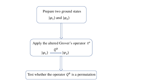
Figure 2: Procedure of algorithm

V The eigenstate preparing via adiabatic quantum evolution

The adiabatic quantum algorithm can be realized on quantum computer. The adiabatic quantum algorithm is usually used for combinational optimization problem. In this paper, we apply it to prepare the eigenvector of the Hamiltonian defined by the adjacency matrix. The time depend Hamiltonian of adiabatic quantum algorithm has the formatFarhi

$$H\left(t\right)=\left({1-\frac{t}{T}}\right){H_{i}}+\left({\frac{t}{T}}\right){H_{P}}$$ (5)

$H_{i}$ is the initial Hamiltonian, $H_{P}$ is the ending Hamiltonian which is defined relying on specific problems. Here, we define that

$${H_{P}}={A_{1}}+I-\xi\left|v\right\rangle\left\langle v\right|,$$ (6)

or

$${H_{P}}={A_{2}}+I-\xi\left|w\right\rangle\left\langle w\right|,$$ (7)

Let $s=\frac{t}{T}$, the eigenvalues of $H(t)$ are $\mu_{1}(s)<,\ldots,\mu_{N}(s)$, and the eigenvectors are $\left|\mu_{1}(s)\right>,\ldots,\left|\mu_{1}(s)\right>$. The evolution time satisfies

$$T\geq\frac{\epsilon}{g_{min}^{2}}$$ (8)

where

$${g_{\min}}=\mathop{\min}\limits_{0\leq t\leq 1}\left({\mu\left(1\right)-\mu\left(0\right)}\right),$$ (9)

and

$$\varepsilon=\mathop{\max}\limits_{0\leq t\leq 1}\left|{\left\langle{\mu\left(1\right)}\right|\frac{{dH\left(s\right)}}{{ds}}\left|{\mu\left(0\right)}\right\rangle}\right|.$$ (10)

When $\xi\ll 1$, $\mu\left(1\right)\approx\mathop{\min}\limits_{j}\left|{{\lambda_{j}}+1}\right|$. Choosing a proper initial Hamiltonian that $\mu(0)=c$, such that c is far less than $\mu(1)$. Since $\varepsilon\geq 1$, the evolution time reaches

$$T\geq\frac{1}{{{{\left({\mathop{\min}\limits_{j}\left|{{\lambda_{j}}+1}\right|}\right)}^{2}}}}.$$

From the above formula, the evolution time is not very long. Hence, in the analysis of time complexity, the preparing time of eigenvectors can be ignored. Note that the initial eigenvector mustn’t be the equal superposition state, since equal superposition state is approximately equal to another eigenvector of $H_{P}$ when The parameter $\xi$ be taken to a small enough value.

VI Finding permutation via an altered Grover algorithm

In the previous section, we have illustrated that the procedure of preparing the ground state of adjacency matrix of isomorphic equivalent graph. Now we have such two ground states, how to check whether there exists a permutation matrix that can transform them each other. Our approach isn’t checking every permutation in the symmetric group $S_{n}$, but directly find what a unitary matrix can transform one eigenvector to another one. We adopt an altered Grover’s algorithm to determine that unitary transform. The Grover’s original algorithm can be found in literature Grover (1996), or one can find the algorithm version described by unitary matrix in literature Williams (2010). we describe the altered Grover’s algorithm by the way of the latter.

Now we have the two eigenvectors $\left|\varphi_{1}\right>$ and $\left|\varphi_{2}\right>$, no matter if the two graphs are isomorphic $\left<\varphi_{1}|\varphi_{2}\right>\neq 0$. By using the altered Grover’s algorithm, $\left|\varphi_{1}\right>$($\left|\varphi_{2}\right>$) can be transformed to $\left|\varphi_{2}\right>$($\left|\varphi_{1}\right>$). The algorithm procedures are listed below:

Step (i). Given two oracles, construct the iterative operator $Q=-U{{\bf{1}}_{s}}{U^{\dagger}}{{\bf{1}}_{t}}$, where $\left|s\right>=\left|\varphi_{1}\right>$ is the initial state, $\left|s\right>=\left|\varphi_{2}\right>$ is the target state, ${{\bf{1}}_{s}}=I-2\left|s\right\rangle\left\langle s\right|$ and ${{\bf{1}}_{t}}=I-2\left|t\right\rangle\left\langle t\right|$ are constructed relied on the oracles, $U$ is a unitary operator satisfies that $\left\langle{{\varphi_{1}}}\right|U\left|{{\varphi_{2}}}\right\rangle\neq 0$.

Step (ii). Iterative execution the operator $k=\frac{\pi}{4}\sqrt{N}$ times, namaly $\left|\phi\right\rangle={Q^{k}}U\left|s\right\rangle$.

Step (iii). Checking that whether $\left\langle{{\varphi_{2}}}\right.\left|\phi\right\rangle\approx 1$ is valid, if yes, turn to Step (iv), otherwise, turn to Step (iii).

Step (iv). Testing whether the operator $Q^{k}$ is a permutation matrix. If yes, then the given two graphs are isomorphic, otherwise the given graphs are non-isomorphic.

Although we have prepared the two ground states in some format Qbit, we don’t know what they are. Hence, we need two oracles in our algorithm and the original Grover’s algorithm only needs one, since we call it the altered Grover’s algorithm. Checking whether a matrix is a permutation can be realized by quantum algorithm just involved the computational basis state. We first need prepare a group of computational basis $\left|j\right>(j=0,...,N-1)$, which can be written is format of vector

$$\left|0\right\rangle=\left[{\begin{array}[]{*{20}{c}}1\\ 0\\ \vdots\\ 0\end{array}}\right],\left|1\right\rangle=\left[{\begin{array}[]{*{20}{c}}0\\ 1\\ \vdots\\ 0\end{array}}\right],\ldots,\left|{N-1}\right\rangle=\left[{\begin{array}[]{*{20}{c}}0\\ 0\\ \vdots\\ 1\end{array}}\right]$$

.

Then, we let the operator $Q^{k}$ acts on every basis vector and measure the result. If the result vectors are all basis states and there are no one pair of them are equal, then the matrix is a permutation. In this manner, we will spend $N$ time since the number of computational basis vector is $N$. Checking all pairs of basis vectors will cost $O(N^{2})$.

VII Time complexity analysis

The algorithm contains three main steps. In the first step, we need prepare $N+1$ ground statesat most. Since the time of preparing one ground state is far less than the time of other steps. In the second step, one need to transform the two ground states by the Grover algorithm, for one round the time is $k=\frac{\pi}{4}\sqrt{N}$. In the third step, we need check that if the matrix $Q^{k}$ is a permutation, we need cost $N^{2}$ time in one turn. The whole procedure, we will do $N$ turn for the worst case that we will check all vertices in the second given graph. So worst time complexity is $O(N^{3})$.

VIII Conclusion

In this work, we put forward a quantum algorithm for GI problem. The time complexity of the algorithm is polynomial. We introduce the isomorphic equivalent graph, and present several theorems for GI test. Via that kind of graph, we transform the GI problem given graphs to GI problem of isomorphic equivalent graphs. By the transformation, the least eigenvalue of the adjacency matrix becomes simple and the corresponding ground state is non-degenerate. That ground state can be efficaciously prepared in a short time by adiabatic quantum evolution. Then, by using the altered Grover algorithm, we can find the transformation matrix between the two ground states. If the given two graph are just co-spectrum but not isomorphic, then that matrix is no longer a permutation matrix. In the original Grover’s algorithm, one needs an oracle, but in the altered Grover’s algorithm we need two oracles. Theoretically, if we can prepare the eigenvector, then the oracle can be made. The work of oracle making is not the main part of our algorithm just as in Grover algorithm.

References

• Kobler et al. (2012) Johannes Kobler, Uwe Schöning, and Jacobo Torán. The graph isomorphism problem: its structural complexity. Springer Science &amp; Business Media, 2012.
• McKay et al. (1981) Brendan D McKay et al. Practical graph isomorphism. 1981.
• Babai (2016) László Babai. Graph isomorphism in quasipolynomial time. In Proceedings of the forty-eighth annual ACM symposium on Theory of Computing, pages 684–697. ACM, 2016.
• Arora and Barak (2009) Sanjeev Arora and Boaz Barak. Computational complexity: a modern approach. Cambridge University Press, 2009.
• Rudolph (2002) Terry Rudolph. Constructing physically intuitive graph invariants. arXiv preprint quant-ph/0206068, 2002.
• Shiau (2005) SY Shiau. S.-y. shiau, r. joynt, and sn coppersmith, quantum inf. comput. 5, 492 (2005). Quantum Inf. Comput., 5:492, 2005.
• Gamble et al. (2010) John King Gamble, Mark Friesen, Dong Zhou, Robert Joynt, and SN Coppersmith. Two-particle quantum walks applied to the graph isomorphism problem. Physical Review A, 81(5):052313, 2010.
• Shiau et al. (2003) Shiue-yuan Shiau, Robert Joynt, and Susan N Coppersmith. Physically-motivated dynamical algorithms for the graph isomorphism problem. arXiv preprint quant-ph/0312170, 2003.
• Berry and Wang (2011) Scott D Berry and Jingbo B Wang. Two-particle quantum walks: Entanglement and graph isomorphism testing. Physical Review A, 83(4):042317, 2011.
• Smith (2010) Jamie Smith. k-boson quantum walks do not distinguish arbitrary graphs. arXiv preprint arXiv:1004.0206, 2010.
• Gaitan and Clark (2014) Frank Gaitan and Lane Clark. Graph isomorphism and adiabatic quantum computing. Physical Review A, 89(2):022342, 2014.
• Hen and Young (2012) Itay Hen and AP Young. Solving the graph-isomorphism problem with a quantum annealer. Physical Review A, 86(4):042310, 2012.
• Tamascelli and Zanetti (2014) Dario Tamascelli and Luca Zanetti. A quantum-walk-inspired adiabatic algorithm for solving graph isomorphism problems. Journal of Physics A: Mathematical and Theoretical, 47(32):325302, 2014.
• Cvetković et al. (1980) Dragoš M Cvetković, Michael Doob, and Horst Sachs. Spectra of graphs: theory and application, volume 87. Academic Pr, 1980.
• Cvetkovic et al. (1997) Dragos Cvetkovic, Dragoš M Cvetković, Peter Rowlinson, and Slobodan Simic. Eigenspaces of graphs, volume 66. Cambridge University Press, 1997.
• (16) E Farhi. E. farhi, j. goldstone, s. gutmann, and m. sipser, quantum computation by adiabatic evolution, arxiv: quant-ph/0001106. Quantum computation by adiabatic evolution.
• Grover (1996) Lov K Grover. A fast quantum mechanical algorithm for database search. In Proceedings of the twenty-eighth annual ACM symposium on Theory of computing, pages 212–219. ACM, 1996.
• Williams (2010) Colin P Williams. Explorations in quantum computing. Springer Science &amp; Business Media, 2010.