Floating-Point Calculations on a Quantum Annealer:
Division and Matrix Inversion

Abstract

Systems of linear equations are employed almost universally across a wide range of disciplines, from physics and engineering to biology, chemistry and statistics. Traditional solution methods such as Gaussian elimination become very time consuming for large matrices, and more efficient computational methods are desired. In the twilight of Moore’s Law, quantum computing is perhaps the most direct path out of the darkness. There are two complementary paradigms for quantum computing, namely, gated systems and quantum annealers. In this paper, we express floating point operations such as division and matrix inversion in terms of a quadratic unconstrained binary optimization (QUBO) problem, a formulation that is ideal for a quantum annealer. We first address floating point division, and then move on to matrix inversion. We provide a general algorithm for any number of dimensions, but we provide results from the D-Wave quantum anneler for $2\times 2$ and $3\times 3$ general matrices. Our algorithm scales to very large numbers of linear equations. We should also mention that our algorithm provides the full solution the the matrix problem, while HHL provides only an expectation value.

I Introduction

Systems of linear equations are employed almost universally across a wide range of disciplines, from physics and engineering to biology, chemistry and statistics. An interesting physics application is computational fluid dynamics (CFD), which requires inverting very large matrices to advance the state of the hydrodynamic system from one time step to the next. An application of importance in biology and chemistry would include the protein folding problem. For large matrices, Gaussian elimination and other standard techniques becomes too time consuming, and therefore faster computational methods are desired. As Moore’s Law draws to a close, quantum computing offers the most direct path forward, and perhaps the most radical path. In a nutshell, quantum computers are physical systems that exploit the laws of quantum mechanics to perform arithmetic and logical operations exponentially faster than a conventional computer. In the words of Harrow, Hassidim, and Lloyd (HHL) hhl , “quantum computers are devices that harness quantum mechanics to perform computations in ways that classical computers cannot.” There are currently two complementary paradigms for quantum computing, namely, gated systems and quantum annealers. Gated systems exploit the deeper properties of quantum mechanics such coherence, entanglement and non-locality, while quantum annealers take advantage of tunneling between metastable states and the ground state. In Ref. hhl , HHL introduces a gated method by which the inverse of a matrix can be computed, and Refs. ref2013a ; ref2013b ; ref2013c provide implementations of the algorithm to invert $2\times 2$ matrices. Gated methods are limited by the relatively small number of qubits that can be entangled into a fully coherent quantum state, currently of order $32$ or so. An alternative approach to quantum computing is the quantum anneler fggs , which takes advantage of quantum tunneling between metastable states and the ground state. The D-Wave Quantum Annealers have reached capacities of $2000+$ qubits, which suggests that quantum annealers could be quite effective for linear algebra with hundreds to thousands of degrees of freedom. In this paper, we express floating point operations such as division and matrix inversion as quadratic unconstrained binary optimization (QUBO) problems, which are ideal for a quantum annealer. We should mention that our algorithm provides the full solution the the matrix problem, while HHL provides only an expectation value. Furthermore, our algorithm places no contraints on the matrix that we are inverting, such as a sparcity condition.

The first step in mapping a general problem to a QUBO problem begins with constructing a Hamiltonian that encodes the logical problem in terms of a set of qubits. Next, it will be necessary to “embed” the problem on the chip, first by mapping each logical qubit to a collection or “chain” of physical qubits, and then by determining parameter settings for all the physical qubits, including the chain couplings. We have implemented our algorithms on the D-Wave 2000Q and 2X chips, illustrating that division and matrix inversion can indeed be performed on an existing quantum annealer. The algorithms that we propose should scale quite well for large numbers of equations, and should be applicable to matrix inversion of relatively high order (although probably not exponentially higher order as in HHL).

Before examining the various algorithms, it is useful to review the basic formalism and to establish some notation. The general problem starts with a graph ${\cal G}=({\cal V},{\cal E})$, where ${\cal V}$ is the vertex set and ${\cal E}$ is the edge set. The QUBO Hamiltonian on ${\cal G}$ is defined by

$$H_{\scriptscriptstyle{\cal G}}[Q] = \sum_{r\in{\cal V}}A_{r}\,Q_{r}+\sum_{rs\in{\cal E}}B_{rs}\,Q_{r}Q_{s}\ ,$$ (1)

with $Q_{r}\in\{0,1\}$ for all $r\in{\cal V}$. The coefficient $A_{r}$ is called the weight at vertex $r$, while the coefficient $B_{rs}$ is called the strength between vertices $r$ and $s$. It might be better to call (1) the objective function rather than the Hamiltonian, as $H_{\scriptscriptstyle{\cal G}}$ is a real-valued function and not an operator on a Hilbert-space. However, it is easy to map (1) in an equivalent Hilbert space form,

$$\hat{H}_{\scriptscriptstyle{\cal G}} = \sum_{r\in{\cal V}}A_{r}\,\hat{Q}_{r}+\sum_{rs\in{\cal E}}B_{rs}\,\hat{Q}_{r}\hat{Q}_{s}\ ,$$ (2)

where $\hat{Q}_{r}|Q\rangle=Q_{r}|Q\rangle$ for all $r\in{\cal V}$, and $|Q\rangle\in{\cal H}$ for Hilbert space $\cal H$. The hat denotes an operator on the Hilbert space, and $Q_{r}$ is the corresponding Eigenvalue of $\hat{Q}_{r}$ with Eigenstate $|Q\rangle$. Consequently, we can write

$$\hat{H}_{\scriptscriptstyle{\cal G}}|Q\rangle=H_{\scriptscriptstyle{\cal G}}[Q]\,|Q\rangle\ ,$$ (3)

and we use the terms Hamiltonian and objective function interchangeably. By the QUBO problem, we mean the problem of finding the lowest energy state $|Q\rangle$ of the Hamiltonian (2), which corresponds to minimizing Eq. (1) with respect to the $Q_{r}$. This is an NP-hard problem uniquely suited to a quantum annealer. Rather than sampling all $2^{\#{\cal V}}$ possible states, quantum tunneling finds the most likely path to the ground state by minimizing the Euclidian action. In the case of the D-Wave 2X chip, the number of distinct quantum states is of order the insanely large number $2^{1000}$, and the ground state is selected from this jungle of quantum states by tunneling to those states with a smaller Euclidean action.

The Ising model Ising1925 is perhaps the quintessential physical example of a QUBO problem, and indeed, is one of the most studied systems in statistical physics. The Ising model consists of a square lattice of spin-1/2 particles with nearest neighbor spin-spin interactions between sites $r$ and $s$, and when the system is immersed in a nonuniform magnetic field, this introduces coupling terms at individual sites $r$, thereby producing a Hamiltonian of the form

$$H_{\scriptscriptstyle{\cal G}}[J] = \sum_{r\in{\cal V}}B_{r}\,J_{r}+\sum_{rs\in{\cal E}}J_{rs}\,J_{r}J_{s}\ ,$$ (4)

where $J_{r}=\pm 1/2$. The Ising problem is connected to the QUBO problem by $J_{r}=Q_{r}-1/2$.

For floating point division to $R$ bits of resolution, the graph ${\cal G}$ is in fact just the fully connected graph $K_{\rm\scriptscriptstyle R}$. In terms of vertex and edge sets, we write $K_{\rm\scriptscriptstyle R}=({\cal V}_{\rm\scriptscriptstyle R},{\cal E}_{\rm\scriptscriptstyle R})$, and Fig. 1 illustrates $K_{8}$ and $K_{4}$.

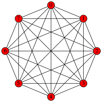
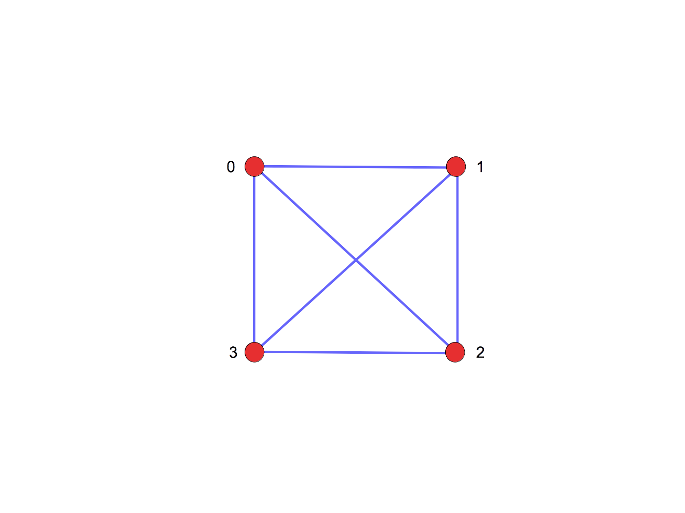
Figure 1: The left panel shows the fully connected graph $K_{8}$ and the right panel shows the corresponding graph $K_{4}$. To perform a calculation to 8-bit accuracy requires the connectivity of $K_{8}$. We take the vertex and edge sets for be $K_{8}$ to ${\cal V}_{8}=\{0,1,2,\cdots,7\}$ and ${\cal E}_{8}=\{\{0,1\},\{0,2\},\cdots,\{0,7\},\{1,2\},\{1,3\},\cdots,\{\,6,7\}\,\}$. To perform a calculation to 4-bit accuracy requires $K_{4}$ connectivity, and similarly, the vertex and edge sets for $K_{4}$ are ${\cal V}_{4}=\{0,1,2,3\}$ and ${\cal E}_{4}=\{\{0,1\},\{0,2\},\{0,3\},\{1,2\},\{1,3\},\{2,3\}\}$.

The left panel shows the completely connected graph $K_{8}$, with vertex and edge sets

$${\cal V}_{8} = \{0,1,2,\cdots,7\}$$ (5)

$${\cal E}_{8} = \{\{0,1\},\{0,2\},\cdots,\{0,7\},\{1,2\},\cdots,\{1,7\},\cdots,\{\,6,7\}\,\}\ ,$$

while the right panel shows the $K_{4}$ graph,

$${\cal V}_{4} = \{0,1,2,3\}$$ (7)

$${\cal E}_{4} = \{\{0,1\},\{0,2\},\{0,3\},\{1,2\},\{1,3\},\{2,3\}\}\ .$$ (8)

Just as 8-bits is called a word, 4-bits is called a nibble. As we will also see, the dynamic range of the D-Wave is most directly suitable to $K_{4}$, and consequently the connectivity of $K_{4}$ gives a quantum nibble.

Let us remark about our summation conventions. Rather than summing over an edge set,

$$H[Q] = \sum_{r\in{\cal V}_{\rm\scriptscriptstyle R}}A_{r}\,Q_{r}+\sum_{rs\in{\cal E}_{\rm\scriptscriptstyle R}}B_{rs}\,Q_{r}Q_{s}$$ (9)

$$= \sum_{r=0}^{R-1}A_{r}\,Q_{r}+\sum_{r=0}^{R-1}\sum_{s>r}^{R-1}B_{rs}\,Q_{r}Q_{s}\ ,$$ (10)

we find it convenient to sum over all values of $r$ and $s$ taking $B_{rs}$ to be symmetric. In this case, the double sum differs by a factor of two relative to summing over the edge set of the graph,

$$H[Q] = \sum_{r=0}^{R-1}A_{r}\,Q_{r}+\sum_{r=0}^{R-1}\sum_{s=0}^{R-1}\frac{1}{2}\,B_{rs}\,Q_{r}Q_{s}\ .$$ (11)

Furthermore, for $r=s$, there will be a linear contribution from the idempotency condition $Q_{r}^{2}=Q_{r}$, so that

$$H[Q] = \sum_{r=0}^{R-1}\left[A_{r}+\frac{1}{2}\,B_{rr}\right]\,Q_{r}+\sum_{r=0}^{R-1}\sum_{s\neq r,s=0}^{R-1}\frac{1}{2}\,B_{rs}\,Q_{r}Q_{s}\ .$$ (12)

We can write this as

$$H[Q] = \sum_{r=0}^{R-1}\tilde{A}_{r}\,Q_{r}+\sum_{r=0}^{R-1}\sum_{s\neq r,s=0}^{R-1}\tilde{B}_{rs}\,Q_{r}Q_{s}\ .$$ (13)

II Floating Point Division on a Quantum Annealer

II.1 Division as a QUBO Problem

In this section we present an algorithm for performing floating point division on a quantum annealer. Given two input parameters $m$ and $y$ to $R$-bits of resolution, the algorithm calculates the ratio $y/m$ to $R$ bits of resolution. The corresponding division problem can be represented by the linear equation

$$m\cdot x-y=0\ ,$$ (14)

which has the unique solution

$$x=y/m\ .$$ (15)

Solving (14) on a quantum annealer amounts to finding an objective function $H(x)$ whose minimum corresponds to the solution that we are seeking, namely (15). Although the form of $H(x)$ is not unique, for this work we employ the simple real-valued quadratic function

$$H(x;m,y)=\big{(}m\,x-y\big{)}^{2}\ ,$$ (16)

where $m$ and $y$ are continuous parmeters. For an ideal annealer, we do not have to concern ourselves with the numerical range and resolution of the parameters $m$ and $y$; however, for a real machine such as the D-Wave, this is an important consideration. For a well-conditioned matrix, we require that the parameters $m$ and $y$ possess a numerical range that spans about an order of magnitude, from approximately 0.1 to 1.0. This provides about 3 to 4 bits of resolution: $1/2^{0}=1$, $1/2^{1}=0.5$, $1/2^{2}=0.25$, and $1/2^{3}=0.125$. The dynamic range and the connectivity both impact the resolution of a calculation.

To proceed, let us formulate floating point division as a quadratic unconstrained binary optimization (QUBO) problem. The algorithm starts by converting the real-valued number $x$ in (16) into an $R$-bit binary format, while the numbers $m$ and $y$ remain real valued parameters of the objective function. For any number $\chi\in[0,2)$, the binary representation accurate to $R$ bits of resolution can be expressed by $[Q_{0}.Q_{1}Q_{2}\cdots Q_{\scriptscriptstyle R-1}]_{2}$, where $Q_{r}\in\{0,1\}$ is value of the $r$-th bit, and the square bracket indicates the binary representation.  It is more algebraically useful to express this in terms of the power series in $2^{-r}$,

$$\chi = \sum_{r=0}^{R-1}2^{-r}\,Q_{r}\ .$$ (17)

In order to represent negative number, we perform the binary offset

$$x = 2\chi-1\ ,$$ (18)

where $x\in[-1,3)$. The objective function now takes the form

$$H(\chi) = 4m^{2}\chi^{2}-4m(m+y)\chi+(m+y)^{2}\ .$$ (19)

The constant term $(m+y)^{2}$ can be dropped when finding the minimum of (19), but we choose to keep it for completeness. Equation (17) provides a change of variables $\chi=\chi[Q]$ (where $Q$ is the collection of the $Q_{r}$), and this allows us to express (16) in the form

$$H[Q] = \sum_{r=0}^{R-1}A_{r}\,Q_{r}+\sum_{r=0}^{R-1}\sum_{s\neq r,s=0}^{R-1}B_{rs}\,Q_{r}Q_{s}\ .$$ (20)

In the notation of graph theory, we would write

$$H[Q] = \sum_{r\in{\cal V}_{\rm\scriptscriptstyle R}}A_{r}\,Q_{r}+\sum_{rs\in{\cal E}_{\rm\scriptscriptstyle R}}\frac{1}{2}\,B_{rs}\,Q_{r}Q_{s}\ ,$$ (21)

where ${\cal V}_{\rm\scriptscriptstyle R}=\{0,1,2,\cdots,R-1\}$ is the vertex set, and ${\cal E}_{\rm\scriptscriptstyle R}$ is the edge set. We often employ an abuse of notation and write $rs\in{\cal E}_{\rm\scriptscriptstyle R}$ to mean $\{r,s\}\in{\cal E}_{\rm\scriptscriptstyle R}$. We should also use the notation $B_{\{r,s\}}$, but instead we write $B_{rs}$. Since the order of the various elements of a set are immaterial, we require $B_{rs}$ to be symmetric in $r$ and $s$. Rather than summing over the edge sets $rs\in{\cal E}_{\rm\scriptscriptstyle R}$, we employ the double sum $\sum_{r\neq s}$, which introduces a relative factor of two in the convention for the strengths $B_{rs}$. The goal of this section is to find $A_{r}$ and $B_{rs}$ in terms of $m$ and $y$.

Note that we can generalize the simple binary offset (17) if we scale and shift $\chi\in[0,2)$ by

$$x = c\chi-d\ ,$$ (22)

so that $x\in[-d,2c-d)$. When $d>0$ and $c>d/2$, the domain of $x$ always contains a positive and negative region, and the precise values for $d$ and $c$ can be chosen based on the specifics of the problem. For Eq. (22), the objective function takes the form

$$H(\chi) = 4m^{2}c^{2}\,\chi^{2}-4mc\,(m+y)\chi+(md+y)^{2}\ .$$ (23)

For simplicity of notation, this paper employs the simple binar offset (18), although our Python interface to the D-Wave quantum annealer employs the generalized form (23).

Equation (17) allows us to express the quadratic term in $\chi$ as

$$\chi^{2}=\sum_{r=0}^{R-1}\sum_{s=0}^{R-1}2^{-r-s}Q_{r}Q_{s}=\sum_{r=0}^{R-1}\sum_{s\neq r,s=0}^{R-1}2^{-r-s}Q_{r}Q_{s}+\sum_{r=0}^{R-1}2^{-2r}Q_{r}\ ,$$ (24)

where we have used the idempotency condition $Q_{r}^{2}=Q_{r}$ along the diagonal in the last term of (24). Substituting the forms (17) and (24) into (19) provides the Hamiltonian

$$H[Q] = \sum_{r=0}^{R-1}4m\,2^{-r}\Big{[}m\,2^{-r}-(y+m)\Big{]}Q_{r}+\sum_{r=0}^{R}\sum_{s\neq r,s=0}^{R-1}4m^{2}\,2^{-r-s}\,Q_{r}Q_{s}\ ,$$ (25)

and the Ising coefficients in (20) can be read off:

$$A_{r} = 4m\,2^{-r}\Big{[}m\,2^{-r}-(y+m)\Big{]}$$ (26)

$$B_{rs} = 4m^{2}\,2^{-r-s}~{}~{}~{}r\neq s\ .$$ (27)

Because of the double sum over $r$ and $s$ in the objective function in (25), the algorithm requires a graph of connectivity $K_{\rm\scriptscriptstyle R}$. The special cases of $K_{8}$ and $K_{4}$ have been illustrated in Fig. 1. To obtain higher accuracy than the $K_{\rm\scriptscriptstyle R}$ graph allows, we can iterate this procedure in the following manner. Suppose we start with $y_{0}=y$, and we are given a value $y_{n-1}$ with $n>1$, then we advance the iteration to $y_{n}$ in the following manner,

$${\rm solve}~{}~{}mx_{n} = y_{n-1}~{}~{}{\rm for}~{}x_{n}~{}{\rm to}~{}R~{}{\rm bits}$$ (28)

$${\rm calculate~{}the~{}error}~{}~{}y_{n} = y_{n-1}-mx_{n}\ .$$ (29)

Now that we have the value $y_{n}$, we can repeat the process to find $y_{n+1}$, and we can stop the iterative procedure when the desired level of accuracy has been achieved.

II.2 Embedding $\bm{K_{\scriptscriptstyle R}}$ onto the D-Wave Chimera Architecture

The D-Wave Chimera chip consists of coupled bilayers of micro rf-SQUIDs overlaid in such a way that, while relatively easy to fabricate, results in a fairly limited set of physical connections between the qubits. However, by chaining together well chosen qubits in a positively correlated manner, this limitation can largely be overcome. The process of chaining requires that we (i) embed the logical graph onto the physical graph of the chip (for example $K_{4}$ onto $C_{8}$) and that we (ii) assign weights and strengths to the physical graph embedding in such as a way as to preserve the ground state of the logical system. These steps are called graph embedding and Hamiltonian embedding, respectively.

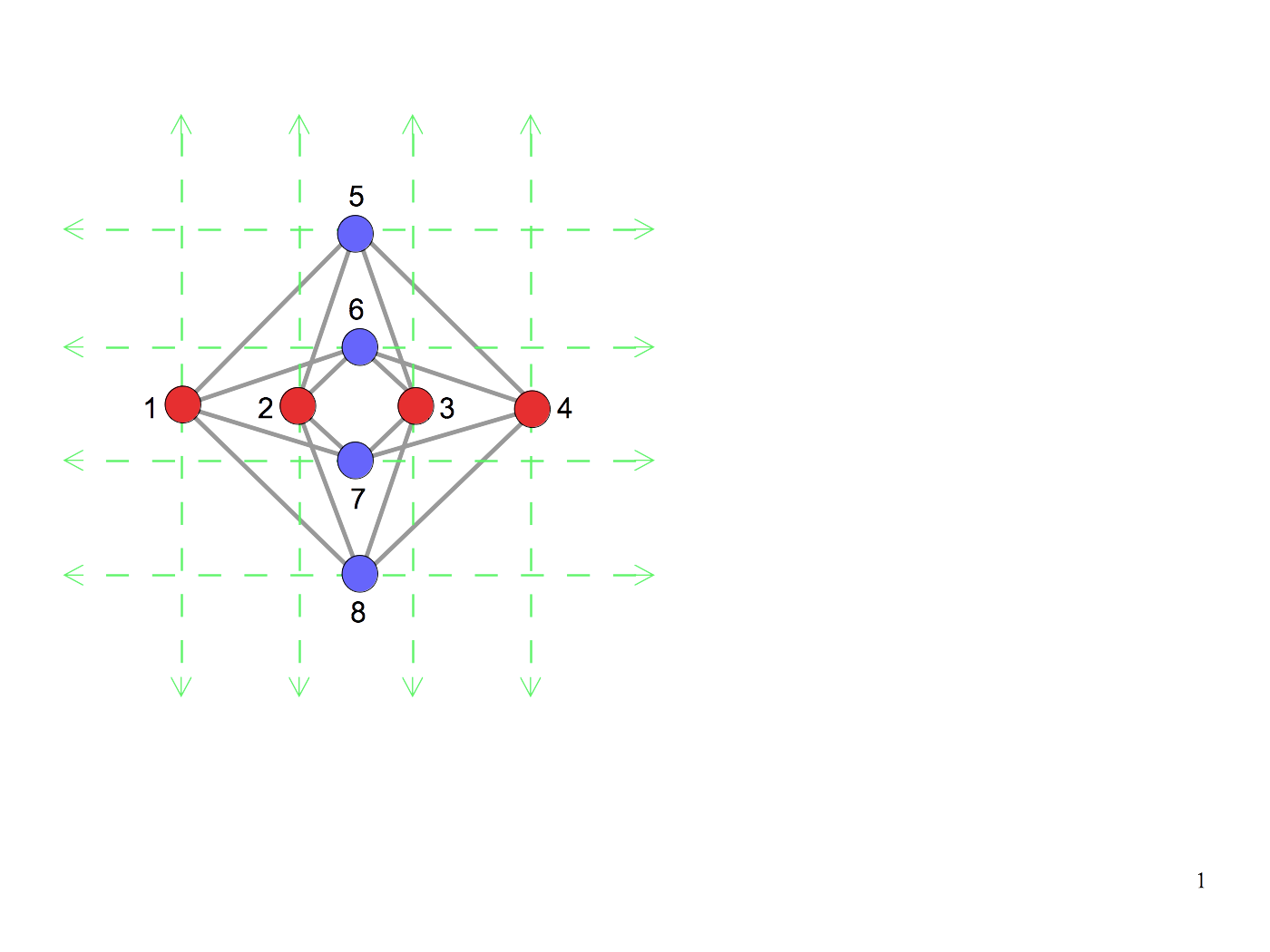
Figure 2: The left panel illustrates the bipartate graph $C_{8}$ in column format, while the right panel illustrates the corresponding graph in cross format, often called a Chimera graph. The gray lines represent direct connections between qubits. The cross format is useful since it minimizes the number intersecting connections. The use of red and blue dots emphasize the bipartate nature of $C_{8}$, as every red dot is connected to every blue dot, while none of the red and blue dots are connected to one another. The vertex set of $C_{8}$ is taken to be ${\cal V}_{8}=\{1,2,\cdots,8\}$ and edge set is ${\cal B}_{8}=\{\{1,5\},\{1,6\},\{1,7\},\{1,8\},\{2,5\},\{2,6\}\cdots\{7,8\}\}$.

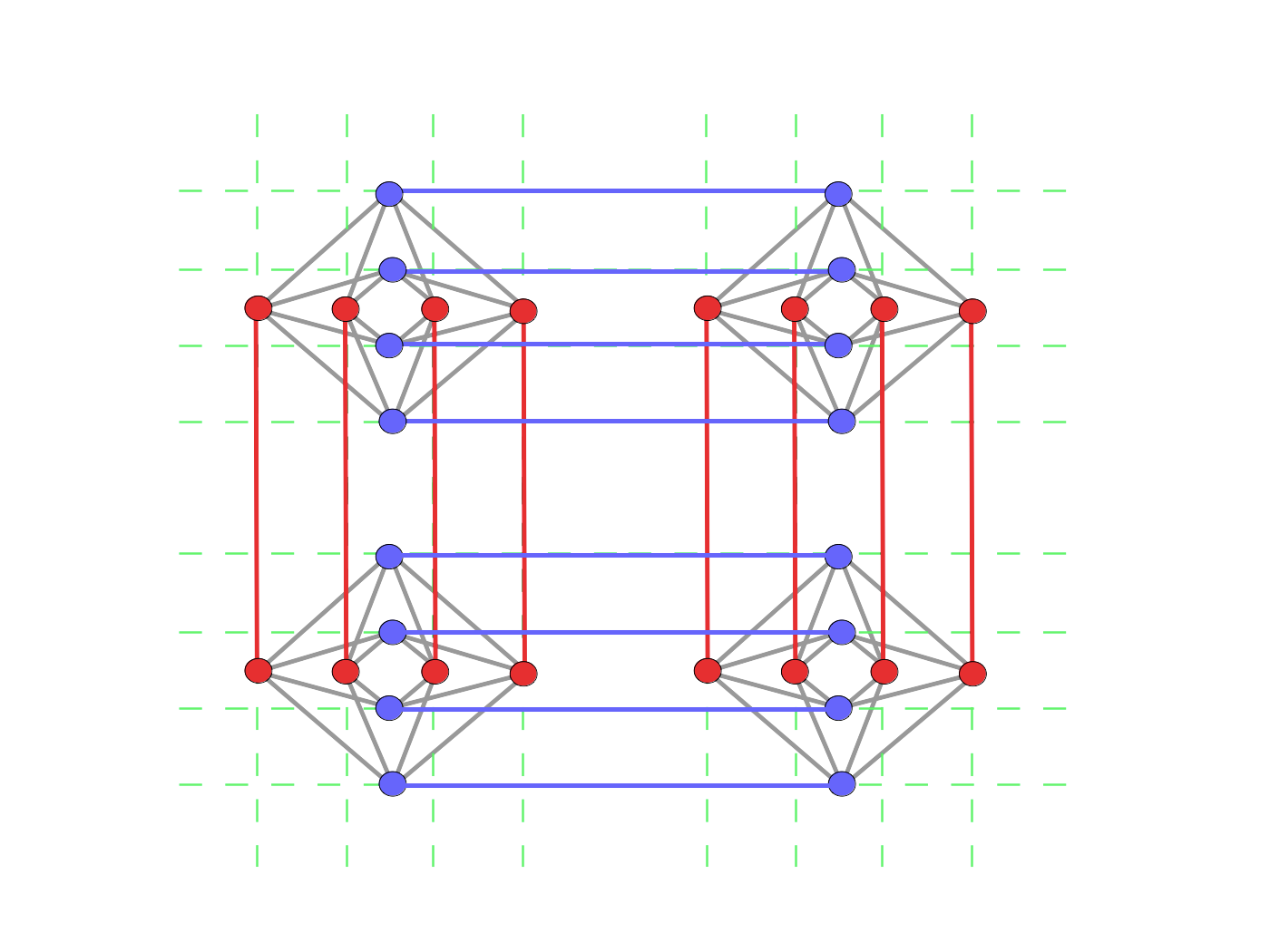
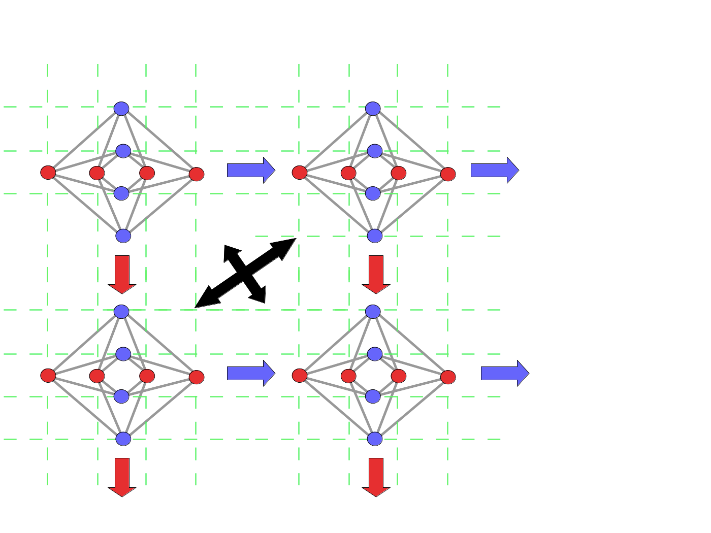
Figure 3: The the left panel shows the connectivity between four $C_{8}$ bipartate Chimera zones, and the right panel illustrates how multiple $C_{8}$ graphs are stitched together along the vertical and horizontal directions to provide thousands of possible qubits. A limitation of this connectivity strategy is that red and blue zones cannot communicate directly with one another, as indicated by the black crossed arrows. The purpose of chaining is to allow communication between the read and blue qubits.

Let us explore the connectivity of the D-Wave Chimera chip in more detail. The D-Wave architecture employs the $C_{8}$ bipartate Chimera graph as its most basic unit of connectivity. This unit cell is illustrated in Fig. 2, and consists of 8 qubits connected in a $4\times 4$ bipartate manner. The left panel of the figure uses a column format in laying out the qubits, and the right panel illustrates the corresponding qubits in a cross format, where the gray lines represent the direct connections between the qubits. The cross format is useful since it minimizes the number intersecting connections. The complete two dimensional chip is produced by replicating $C_{8}$ along the vertical and horizontal directions, as illustrated in Fig. 3, thereby providing a chip with thousands of qubits. The connections between qubits are limited in two ways: (i) by the connectivity of the basic unit cell $C_{8}$ and (ii) by the connectivity between the unit cells across the chip. The bipartate graph $C_{8}=({\cal V}_{8},{\cal B}_{8})$ is formally defined by the vertex set ${\cal V}_{8}=\{1,2,\cdots,8\}$, and the edge set

$${\cal B}_{8} = \big{\{}\{1,5\},\{1,6\},\{1,7\},\{1,8\},\{2,5\},\{2,6\},\{2,7\},\{2,8\},$$ (30)

$$~{}~{}\{3,5\},\{3,6\},\{3,7\},\{3,8\},\{4,5\},\{4,6\},\{4,7\},\{4,8\}\big{\}}.$$

The set ${\cal B}_{8}$ represents the connections between a given red qubit and the corresponding blue qubits in the Figures. The red and blue dots illustrate the bipartate nature of $C_{8}$, as every red dot is connected to every blue dot, while none of the blue and red dots are connected to one another.

We will denote the physical qubits on the D-Wave chip by $q_{\ell}$. For the D-Wave 2000Q there is a maximum of 2048 qubits, while the D-Wave 2X has 1152 qubits. For the example calculation in this text, we only use 10 to 50 qubits. The physical Hamiltonian or objective function takes the form

$$H[q]=\sum_{\ell}a_{\ell}\,q_{\ell}+\sum_{\ell\neq m}2b_{\ell m}\,q_{\ell}q_{m}\ ,$$ (31)

where we have introduced a factor of 2 in the strength to account for the symmetric summation over $r$ and $s$. We will call the qubits $Q_{r}$ of the previous section the logical qubits. To write a program for the D-Wave means finding an embedding of the logical problem onto the physical collection of qubits $q_{\ell}$. If the connectivity of the Chimera graphs were large enough, then the logical qubits would coincide exactly with the physical qubits. However, since the graph $C_{8}$ possesses less connectivity than $K_{4}$, we must resort to chaining on the D-Wave, even for 4-bit resolution. Figure 4 illustrates the $K_{4}$ embedding used by our algorithm, where, as before, the left panel illustrates the bipartate graph in column format, and the right panel illustrates the corresponding graph in cross format.

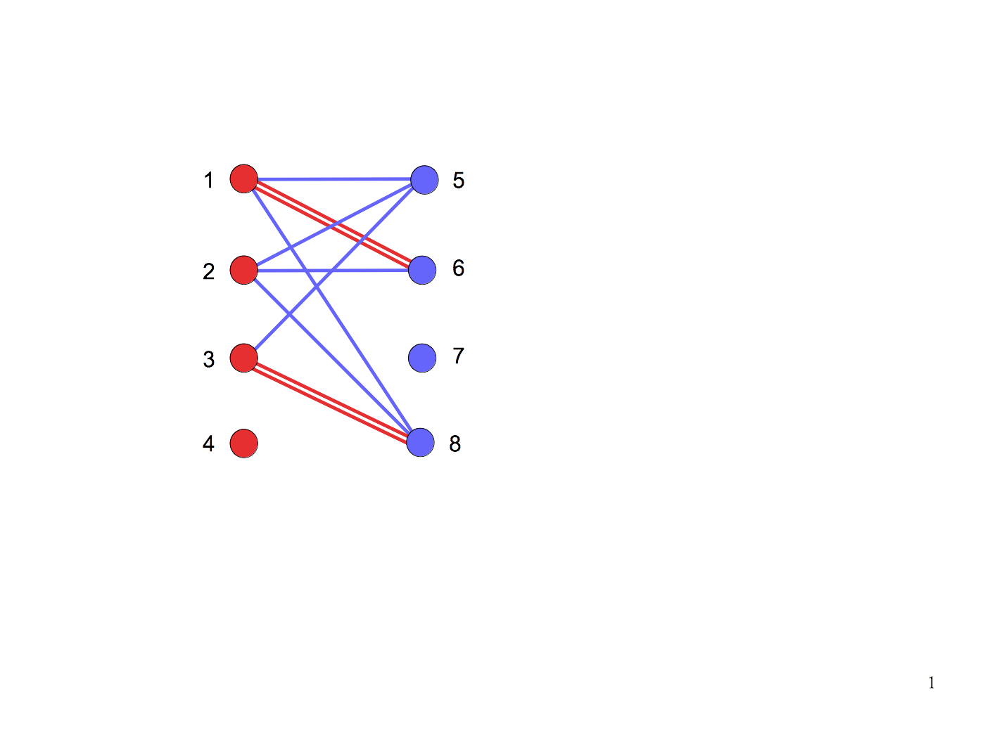
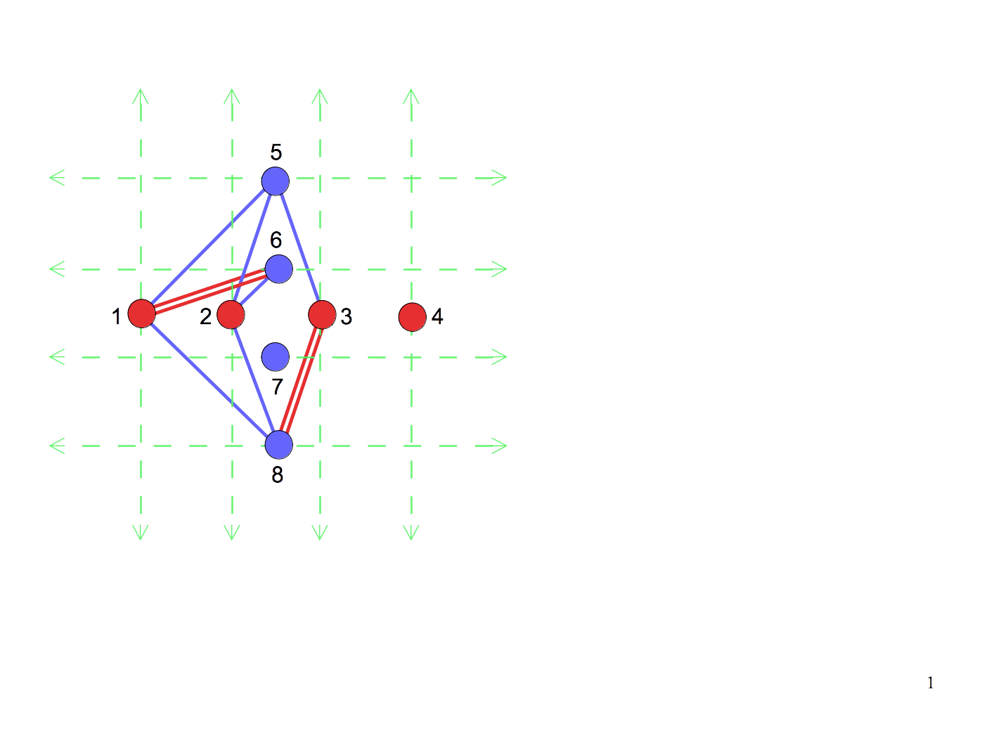
Figure 4: The $K_{4}$ embedding onto $C_{8}$ used in our implementation of 4-bit of division on the D-Wave. The blue lines represent normal connections between qubits, while the red double-lines represent chained qubits, that is to say, qubits that are strictly correlated (and can thereby represent a single logical qubit at a higher level of abstraction). The qubits 1-6 are chained together, as are the qubits 3-8.

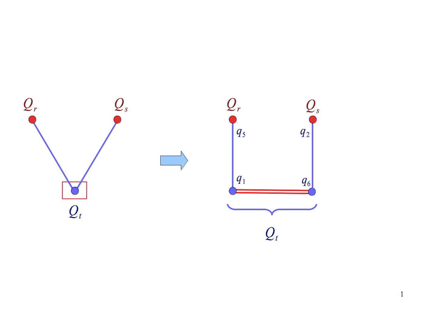
Figure 5: The left panel shows three logical qubits $Q_{r}$, $Q_{s}$, $Q_{t}$ with connectivity between $r$-$t$ and $t$-$s$. The box surrounding qubit $t$ means that it will be modeled by a linear chain of physical qubits, as illustrated in the right panel. The labeling is taken from Fig. 4 for qubits 5-1-6-2, where $Q_{r}$ is mapped to $q_{5}$, $Q_{s}$ is mapped to $q_{2}$, and $Q_{t}$ is split between $q_{1}$ nd $q_{6}$. Qubits $q_{1}$ and $q_{6}$ are chained together to simulate the single logical qubit $Q_{t}$, while qubits $Q_{r}$ and $Q_{s}$ map directly onto physical qubits $q_{5}$ and $q_{2}$.

In Fig. 4 we have labeled the physical qubits by $\ell=1,2,3\cdots 8$, and we wish to map the logical problem involving $Q_{r}\,Q_{s}\,Q_{t}$ onto the four physical qubits $q_{5}\,q_{1}\,q_{6}\,q_{2}$. The embedding requires that we chain together the two qubits 1-6 and 3-8, respectively. We may omit qubits $4$ and $7$ entirely. As illustrated in Fig. 5, the physical qubits $q_{1}$ and $q_{6}$ are chained together to simulate a single logical qubit $Q_{t}$, while qubits $q_{5}$ and $q_{2}$ are mapped directly to the logical qubits $Q_{r}$ and $Q_{s}$, respectively. Qubit $q_{5}$ is assigned the weight $a_{5}=A_{r}$ and the coupling between $q_{5}$ and $q_{1}$ is assigned the value $b_{51}=B_{rt}$. Similarly for qubit $q_{2}$, the vertex is assigned weight $a_{2}=A_{s}$, and strength between $q_{2}$ and $q_{6}$ is $b_{26}=B_{st}$. We must now distribute the logical qubit $Q_{t}$ between $q_{1}$ and $q_{6}$ by assigning the values $a_{1}$, $a_{6}$ and $b_{16}$. We distribute the weight $A_{t}$ uniformly between qubits $q_{1}$ and $q_{2}$, giving $a_{1}=A_{t}/2$ and $a_{6}=A_{t}/2$. We must now choose $b_{16}$. To preserve the energy spectrum, we must shift the values of the weights $a_{1}$ and $a_{6}$. We can do this by adding a counter-term Hamiltonian

$$H^{\rm\scriptscriptstyle CT}=a\,q_{1}+a\,q_{6}+2b_{16}\,q_{1}q_{6}\$$ (32)

to the physical Hamiltonian.

Figure 6: Generalization of Fig. 5 to a chain of $N$ linear qubits. The right panel illustrates the chain coupling parmeters used to create strict correlations of the physical qubits within the chain.

The double lines in Figs. 4 and 5 indicate that two qubits are chained together. This means that the qubits are strictly correlated, i.e. when $q_{1}$ is up then $q_{6}$ is up, and when $q_{1}$ is down then $q_{6}$ is down. This is accomplished by choosing the coupling strength $b_{16}$ to favor a strict correlation; however, to preserve the ground state energy, this also requires shifting the weights for $q_{1}$ and $q_{6}$. For $q_{1}=q_{6}=0$ we have $H^{\rm\scriptscriptstyle CT}=0$. We wish to preserve this condition when $q_{1}=q_{6}=1$, which means $2a+2b=0$. Furthermore, the state $q_{1}=1$ and $q_{6}=0$ must have positive energy, which means $a>0$. Similarly for $q_{1}=0$ and $q_{6}=1$. We therefore choose $a_{1}=a_{6}=\alpha>0$ and $b_{16}=-\alpha$, where $\alpha$ is an arbitrary parameter. This is illustrated in Table. 1.

Table 1: For two qubits the counter-term Hamiltonian is $H^{{\rm\scriptscriptstyle CT}}(q_{1},q_{6})=a\,q_{1}+a\,q_{6}+2b\,q_{1}q_{6}$. The lowest energy state is preserved for $b=-\alpha$ and $a=\alpha$ where $\alpha>0$. We will split the weight $A_{t}$ uniformly across the $N$ chained physical qubits, thereby giving a contribution to the physical Hamiltonian $H_{16}^{t}=A_{t}/2+\alpha\,q_{1}+\alpha\,q_{6}-2\alpha\,q_{1}q_{6}$. The energy spectrum ensures that the two qubits are strictly correlated.

$q_{1}$	$q_{6}$	$H^{{\rm\scriptscriptstyle CT}}$
0	0	0
0	1	$\alpha$
1	0	$\alpha$
1	1	0

A more complicated case is the linear chain of $N$ qubits as shown in Fig. 6. The counter-term Hamiltonian is taken to be

$$H^{\rm\scriptscriptstyle CT}=\sum_{m=1}^{N}a_{m}^{t}\,q^{t}_{m}+\sum_{m=1}^{N-1}b_{m,m+1}^{t}\,q_{m}^{t}q_{m+1}^{t}\ .$$ (33)

Note that $H^{\rm\scriptscriptstyle CT}$ vanishes when $q_{m}=0$ for all $m=1\cdots N$. And conversely, we must arrange the counter-term to vanish when $q_{m}=1$. The simplest choice is to take all weights to be the same and all couplings to be identical. Then, to preserve the ground state when the $q_{r}=1$, we impose

$$a^{t}_{r}=\frac{A_{t}}{N}+\frac{2(N-1)}{N}\,\alpha$$ (34)

$$b^{t}_{r,r+1}=-\alpha$$ (35)

with $\alpha>0$ and $r=1\cdots N$. The first term in $a^{t}_{r}$ distributes the weight $A_{t}$ uniformly across all $N$ nodes in the chain. The second set of terms $b^{t}_{r,r+1}$ ensures that the qubits of the chain are strictly correlated. The counter-term energy is positive and is therefore selected against when the linearly chained qubits are not correlated. Table 2 illustrates the spectrum of the counter-term Hamiltonian for three qubits. We often need to choose large values of $\alpha$, of order 20 or more, to sufficiently separate the states. The uniform spectrum of 4 states with $H^{{\rm\scriptscriptstyle CT}}=a$ in Table 2 arises from a permutation symmetry in $q_{1}$, $q_{2}$, $q_{3}$.

Table 2: For a three qubit chain the counter-term Hamiltonian is $H^{{\rm\scriptscriptstyle CT}}(q_{1},q_{2},q_{3})=a\,q_{1}+a\,q_{2}+a\,q_{3}+2b\,q_{1}q_{2}+2b\,q_{2}q_{3}$, where $a=4\alpha/3$ and $b=-\alpha$. The degeneracy in energy of value $a$ arises from a permutation symmetry in $q_{1}\to q_{2}\to q_{3}$ that preserves the form of the counter-term Hamiltonian.

$q_{1}$	$q_{2}$	$q_{3}$	$H^{\rm\scriptscriptstyle CT}$
0	0	0	0	0
0	0	1	$4\alpha/3$	$a$
0	1	0	$4\alpha/3$	$a$
0	1	1	$2\alpha/3$	$a/2$
1	0	0	$4\alpha/3$	$a$
1	0	1	$8\alpha/3$	$2a$
1	1	0	$2\alpha/3$	$a$
1	1	0	0	0

To review, note that a linear counter-term is represented in Fig. 6. We add a counter-term to break the logical qubits into a chain of physical qubits that preserve the ground state. Let us consider the conditions that we place on the Hamiltonian to ensure strict correlation between the chained qubits. We adjust the values of $A_{r}$ and $B_{rs}$ to ensure that spin alignment is energetically favorable. By slaving several qubits together, we can overcome the limitations of the Chimera connectivity. As a more complex example, consider the four logical qubits of Fig. 7 connected in a circular chains by strengths $B_{12}$, $B_{24}$, $B_{43}$, and $B_{31}$. Suppose the weights are $A_{1}$, $A_{2}$ $A_{3}$ and $A_{4}$. Figure 8 provides an example in which each logical qubit is chained in a linear fashion to the physical qubits.

Figure 7: Four logical qubits $Q_{1}$, $Q_{2}$, $Q_{3}$, $Q_{4}$ in a circular loop with connection strengths $B_{12}$, $B_{24}$ $B_{43}$ and $B_{31}$.

Figure 8: A possible mapping of the logical qubits in Fig. 7 onto the physical device. Each logical qubit is modeled by a linear chain of strictly correlated qubits.

III Matrix Inversion as a QUBO Problem

In this section we present an algorithm for solving a system of linear equations on a quantum annealer. To precisely define the mathematical problem, let $\bm{M}$ be a nonsingular $N\times N$ real matrix, and let $\mathbf{Y}$ be a real $N$ dimensional vector; we then wish to solve the linear equation

$$\bm{M}\cdot\mathbf{x}=\mathbf{Y}\ .$$ (36)

The linearity of the system means that there is a unique solution,

$$\mathbf{x}=\bm{M}^{-1}\cdot\mathbf{Y}\ ,$$ (37)

and the algorithm is realized by specifying an objective function whose ground state is indeed (37). The objective function is not unique, although it must be commensurate with the architecture of the hardware. If the inverse matrix itself is required, it can be constructed by solving (36) for each of the $N$ linearly independent basis vectors for ${\bf Y}$. It is easy to construct a quadratic objective $H({\bf x})$ whose whose minimum is (37), namely

$$H(\mathbf{x}) = \big{(}\bm{M}\mathbf{x}-\mathbf{Y}\big{)}^{2}=\big{(}\bm{M}\mathbf{x}-\mathbf{Y}\big{)}^{\rm\scriptscriptstyle T}\cdot\big{(}\bm{M}\mathbf{x}-\mathbf{Y}\big{)}\ .$$ (38)

In terms of matrix components, this can be written

$$H(\mathbf{x}) = \mathbf{x}^{\rm\scriptscriptstyle T}\bm{M}^{\rm\scriptscriptstyle T}\bm{M}\mathbf{x}-\mathbf{x}^{\rm\scriptscriptstyle T}\bm{M}^{\rm\scriptscriptstyle T}\mathbf{Y}-\mathbf{Y}^{\rm\scriptscriptstyle T}\bm{M}\mathbf{x}+\mathbf{Y}^{\rm\scriptscriptstyle T}\mathbf{Y}$$ (39)

$$= \sum_{ijk=1}^{N}M_{ki}M_{kj}\,x^{i}x^{j}-2\sum_{ij=1}^{N}Y_{j}M_{ji}\,x^{i}+\|\mathbf{Y}\|^{2}\ .$$

Note that $\|\mathbf{Y}\|^{2}$ is just a constant, which will not affect the minimization. In principle all constants can be dropped from the objective function, although we choose to keep them for completeness. One may obtain a floating point representation of each component of $\mathbf{x}=(x^{1},\cdots,x^{\rm\scriptscriptstyle N})^{\rm\scriptscriptstyle T}$ by expanding in powers of $2$ multiplied by Boolean-valued variables $q^{i}_{r}\in\{0,1\}$,

$$\chi^{i} = \sum_{r=0}^{R-1}2^{-r}q^{i}_{r}$$ (40)

$$x^{i} = 2\chi^{i}-1\ .$$ (41)

As before, the domains are give by $\chi^{i}\in[0,2)$ and $x^{i}\in[-1,3)$, and upon expressing ${\bf x}$ as a function the $q_{r}^{i}$ we can recast (39) in the form

$$H[q] = \sum_{i=1}^{N}\sum_{r=0}^{R-1}a_{r}^{i}\,q^{i}_{r}+\sum_{i=1}^{N}\sum_{i\neq j=1}^{N}\sum_{r=0}^{R-1}\sum_{s=0}^{R-1}b_{rs}^{ij}\,q^{i}_{r}q^{j}_{s}\ .$$ (42)

The coefficients $a_{r}^{i}$ are called the weights and the coefficients $b_{rs}^{ij}$ are the interaction strengths. Note that the algorithm requires a connectivity of $K_{\rm\scriptscriptstyle NR}$.

Let us first calculate the product $x^{i}x^{j}$ in (39). From (40) and (41) we find

$$x^{i}x^{j} = \left(2\sum_{r=0}^{R-1}2^{-r}q_{r}^{i}-1\right)\left(2\sum_{r^{\prime}=0}^{R-1}2^{-r^{\prime}}q_{r^{\prime}}^{i}-1\right)$$ (43)

$$= 4\sum_{rr^{\prime}}2^{-(r+r^{\prime})}q_{r}^{i}q_{r^{\prime}}^{j}-4\sum_{r}2^{-r}q_{r}^{i}+1$$

$$= 4\sum_{r\neq r^{\prime}}2^{-(r+r^{\prime})}q_{r}^{i}q_{r^{\prime}}^{j}+4\sum_{r}2^{-2r}q_{r}^{i}-4\sum_{r}2^{-r}q_{r}^{i}+1\ ,$$ (44)

where we have used the idempotency condition $(q_{r}^{i})^{2}=q_{r}^{i}$ in the second term of (44). While the second form is one used by the code, it is more convenient algebraically to use the first form. Substituting (43) into the first term in (39) gives

$$H_{1} \equiv \sum_{ijk}M_{ki}M_{kj}\,x_{i}x_{j}$$ (45)

$$= \sum_{ijk}M_{ki}M_{kj}\,\left\{4\sum_{rr^{\prime}}2^{-(r+r^{\prime})}q_{r}^{i}q_{r^{\prime}}^{j}-4\sum_{r}2^{-r}q_{r}^{i}+1\right\}$$ (46)

$$= 4\sum_{ir}\sum_{js}\sum_{k}2^{-r-s}M_{ki}M_{kj}\,q_{r}^{i}q_{s}^{j}-4\sum_{ir}\sum_{k}2^{-r}M_{ki}M_{ki}\,q_{r}^{i}+\sum_{ijk}M_{ki}M_{kj}\ .$$ (47)

The second term in (39) can be expressed as

$$H_{2} \equiv -2\sum_{ij}Y_{j}M_{ji}\,x_{i}=-2\sum_{ij}Y_{j}M_{ji}\left(2\sum_{r}2^{-r}q_{r}^{i}-1\right)$$ (48)

$$= -4\sum_{ij}\sum_{r}2^{-r}M_{ji}Y_{j}\,q_{r}^{i}+2\sum_{ij}Y_{j}M_{ji}\ .$$ (49)

Adding $H_{1}$ and $H_{2}$ gives

$$H = 4\sum_{ir}\sum_{js}\sum_{k}2^{-r-s}M_{ki}M_{kj}\,q_{r}^{i}q_{s}^{j}-4\sum_{ir}\sum_{k}2^{-r}M_{ki}M_{ki}\,q_{r}^{i}$$ (51)

$$-4\sum_{ij}\sum_{r}2^{-r}M_{ji}Y_{j}\,q_{r}^{i}+2\sum_{ij}Y_{j}M_{ji}+\sum_{ijk}M_{ki}M_{kj}\ .$$

The Ising terms are therefore

$$a_{r}^{i} = 4\cdot 2^{-r}\sum_{k}M_{ki}\left\{2^{-r}M_{ki}-\bigg{(}Y_{k}+\sum_{j}M_{kj}\bigg{)}\right\}$$ (52)

$$b_{rs}^{ij} = 4\cdot 2^{-(r+s)}\sum_{k}M_{ki}\,M_{kj}\ .$$ (53)

The physical qubits in are accessed by a $1$-dimensional linear index, while the logical qubits in are defined in terms of the 2-dimensional indicies $i$ and $r$, where $i=0,1,\cdots,N-1$ and $r=0,1,\cdots,R-1$. To map the logical qubits onto the physical qubits, we re-parameterize the logical qubits by a single index $\ell=0,1,\cdots,NR-1$. Now we define a $1$-$1$ mapping between these indices and the linear index $\ell=0,1,\cdots,N\cdot R-1$. This is just an ordinary linear indexing for $2$-dimensional matrix elements, so we choose the usual row-major linear index mapping,

$$\ell(i,r) = i\cdot R+r$$ (54)

$$M_{\ell} = M_{ir}\ .$$ (55)

The inverse mapping gives the row and column indices as below,

$$i_{\ell} = \lfloor\ell/R\rfloor$$ (56)

$$r_{\ell} = \ell~{}{\rm mod}~{}R\ ,$$ (57)

where $\lfloor n\rfloor$ is the greatest integer less than or equal to $n$. The expression “$\ell~{}{\rm mod}~{}R$” is $\ell$ modulo $R$. This is a $1$-$1$, invertible mapping between each pair of values of $i$ and $r$ in the matrix index space to every value of $\ell$ in the linear qubits index space. We can simply replace sums over all index pairs $i,r$ by a single sum over $\ell$, provided we also rewrite any isolated indices in $i$ and $r$ as functions of $\ell$ via their inverse mapping.

We may summarize this observation in the following formal identity. Given some arbitrary quantity, $A$, that depends functionally upon the tuple $(i,r)$, and possibly upon the individual indices $i$ and $r$, it is trivial to verify that,

$$A[(i,r),i,r]=\sum_{\ell=0}^{N\cdot R-1}A[\ell,i_{\ell},r_{\ell}]\,\delta_{i,i_{\ell}}\delta_{rr_{\ell}}\ ,$$ (58)

where $\ell$, $i_{\ell}$, and $r_{\ell}$ are related as in equations (54)-(57). This identity is useful for formal derivations. For example, we may use it to quickly derive the binary expansion of $x_{i}$ in terms of logical qubits. Inserting (58) into (41) gives,

$$x_{i} = 2\left(\sum_{r=0}^{R-1}2^{-r}\sum_{\ell=0}^{N\cdot R-1}q_{\ell}\,\delta_{i\,i_{\ell}}\delta_{r\,r_{\ell}}\right)-1$$ (59)

$$= 2\sum_{\ell=0}^{N\cdot R-1}2^{-r_{\ell}}\,q_{\ell}\,\delta_{i,i_{\ell}}-1\ .$$

Clearly, $x_{i}$ has non-zero contributions only for those indices corresponding to $i=i_{\ell}=\lfloor\ell/R\rfloor$, that is, only from those qubits within a row in the $q^{i}_{r}$ array. Also, those contributions are summed along that row, i.e., over $r_{\ell}=\ell~{}{\rm mod}~{}R$. This equation will be used to reconstruct the floating-point solution, $\mathbf{x}$, from the components $q_{\ell}$ of the binary solution returned from the D-Wave annealing runs. The weights and strengths now become

$$a_{\ell} = 4\cdot 2^{-r_{\ell}}\sum_{k}M_{k\,i_{\ell}}\left\{2^{-r_{\ell}}M_{k\,i_{\ell}}-(Y_{k}+\sum_{j}M_{kj})\right\}$$ (60)

$$b_{\ell m} = 4\cdot 2^{-(r_{\ell}+r_{\ell^{\prime}})}\sum_{k}M_{k\,i_{\ell}}\,M_{k\,i_{m}}\ .$$ (61)

For a $2\times 2$ matrix to 4-bit accuracy, we need $K_{8}$ ($4\times 2=8$), and to 8-bit accuracy we need $K_{16}$ ($8\times 2=16$). We have inverted matrices up to $3\times 3$ to 4-bit accuracy, which requires $K_{12}$ ($3\times 4=12$). For an $N\times N$ matrix with $R$ bits of resolutions, we must construct linear embeddings of $K_{RN}$. We could generalize this procedure for complex matrices.

IV Calculations

IV.1 Implementation

The methods above were implemented using D-Wave’s Python SAPI interface and tested on a large number of floating-point calculations. Initially, we performed floating-point division on simple test problems with a small resolution. Early on, we discovered that larger graph embeddings tended to produce noisier results. To better understand what was happening we started with a $K_{8}$ graph embedding to represent two floating-point numbers with only four bits of resolution. Since the D-Wave’s dynamic range is limited to about a factor of 10 in the scale of the QUBO parameters, we determined that we could expect no more than 3 to 4 bits of resolution from any one calculation in any event. However, our binary offset representation (40) implies that we should expect no more than 3 bits of resolution in any single run. Indeed, using the $K_{8}$ embedding, we were able to get exact solutions from the annealer for any division problems which had answers that were multiples of 0.25, between -1.0, and 1.0. Problems in this range which had solutions that were not exact multiples of 0.25 resulted in approximate solutions, effectively “rounded” to the nearest of $\pm 0.25$ or $\pm 0.75$. At this point we implemented an iterative scheme that uses the current error, or residual, as a new input, keeping track of the accumulated floating-point solution.

The iteration method has been implemented and tested for floating-point division but we have not yet implemented iteration for matrix inversion. That can be done by using the previous residual (error) as the new inhomogeneous term in the matrix equation. We plan to implement an iterative method in the matrix inversion code soon. However, we already have good preliminary results on matrix inversion that encourages us that this should work reasonably well, at least for well-conditioned matrices. Currently, we are able to solve $2\times 2$ and $3\times 3$ linear equations involving floating-point numbers up to a resolution of 4 bits, and having well-conditioned matrices, exactly for input vectors with elements defined on $[-1,1]$ and that are multiples of $0.25$. Using an example matrix that is poorly-conditioned, we find that it is generally not possible to get the right answer without first doing some sort of pre-conditioning to the matrix. But more importantly, we were able to obtain some insight about why ill-conditioned matrices can be difficult to solve as QUBO problems on a quantum annealer, which gives some hints about how to ameliorate the problem. We will discuss these results, and the effects of ill-conditioning on the QUBO matrix inverse problem below.

IV.1.1 Note on Solution Normalization and Iteration

Allowing both the division and linear equation QUBO solvers to work for arbitrary floating-point numbers, and to allow for iterative techniques, requires normalizing the ratio of the current dividend and the divisor, or the residual and matrix, to a value in a range between $-1$ and $1$. For the division problems, we wanted to avoid “dividing in order to divide”, so we normalized each ratio using the difference between the binary exponents of $\lfloor\mathrm{divisor}\rfloor$ and $\lfloor\mathrm{dividend}\rfloor$. These can be found just by using order comparisons, with no explicit divisions. Adding $1$ to this yields an “offset” - the largest binary exponent of the ratio - to within a factor of $2$ ($\pm 1$ in the offset), which is sufficient for scaling our QUBO parameters as needed. The fact that our QUBO solutions are always returned in binary representation provides a simple way to bound the solution into a range solvable with the annealer by simply shifting the binary representation of the current dividend by a few bits (using the current offset), which is why we refer to the solution exponent as an “offset”. In this way, the solution can easily be guaranteed to be in the correct range without having to perform any divisions in Python. The “offset” is accumulated and used to construct the current approximation to the floating-point solution on each iteration. The iteration process continues until the error of the approximate solution is less than some tolerance specified by the user.

IV.2 Results for Division

First, we present some examples for division without iteration. We used a $K_{4}$ graph embedding for expanding the unknown $x$ up to a resolution of 4 bits. However using the binary offset representation we can only get a true precisions of 3 bits. We solved the simple division problem,

$$x = \frac{y}{m}\ .$$ (62)

IV.2.1 Basic Division Solver

Table 3 gives an extensive list of tested exact solutions returned by the floating-point annealing algorithm on the D-Wave machine using the $K_{4}$ graph embedding with an effective binary resolution of $3$, corresponding to the multiples of $0.25$ in the range $[-1,1]$. The “Ground State” column lists the raw binary vector solutions, corresponding to the expansion in Eq (18). It is easy to check from Eqs. (18) and (17) that these give the floating-point solutions found in the corresponding “D-Wave Solution” column. In all of these cases, values of $\alpha\geq 0.5$ yielded the solution exactly; however, $\alpha$ is set to 20.0 here because that gives a better approximate solution for the inexact divisions, and faster convergence for the iterated divisions. It does not change the solutions for the exact cases.

Table 3: Exact Quantum Annealed Division Problems to $3$-bit Resolution.

Division Problems with Exact D-Wave Solutions
y	m	x, Exact	x, D-Wave	Ground State	Energy	$\alpha$
-$1.00$	-$1.0$	-$1.00$	-$1.00$	[1,0,0,0]	-2.0	20.0
-$0.50$	-$0.5$	-$1.00$	-$1.00$	[1,0,0,0]	-2.0	20.0
-$1.00$	-1.0	-1.00	-1.00	[0,0,0,0]	-$0.0$	20.0
-1.00	-$1.0$	-1.00	-1.00	[0,0,0,0]	-$0.0$	20.0
-$0.50$	-0.5	-1.00	-1.00	[0,0,0,0]	-$0.0$	20.0
-0.50	-$0.5$	-1.00	-1.00	[0,0,0,0]	-$0.0$	20.0
-$0.75$	-$1.0$	-$0.75$	-$0.75$	[0,1,1,1]	-1.53125	20.0
-0.75	-$1.0$	-0.75	-0.75	[0,0,0,1]	-0.03125	20.0
-$0.75$	-1.0	-0.75	-0.75	[0,0,0,1]	-0.03125	20.0
-$0.50$	-$1.0$	-$0.50$	-$0.50$	[0,1,1,0]	-1.125	20.0
-0.50	-$1.0$	-0.50	-0.50	[0,0,1,0]	-0.125	20.0
-$0.50$	-1.0	-0.50	-0.50	[0,0,1,0]	-0.125	20.0
-$0.25$	-$1.0$	-$0.25$	-$0.25$	[0,1,0,1]	-0.78125	20.0
-0.25	-$1.0$	-0.25	-0.25	[0,0,1,1]	-0.28125	20.0
-$0.25$	-1.0	-0.25	-0.25	[0,0,1,1]	-0.28125	20.0
-$0.25$	-$0.5$	-$0.50$	-$0.50$	[0,1,1,0]	-1.125	20.0
-0.25	-$0.5$	-0.50	-0.50	[0,0,1,0]	-0.125	20.0
-$0.25$	-0.5	-0.50	-0.50	[0,0,1,0]	-0.125	20.0
-$0.00$	$\pm 1.00$	-$0.00$	-$0.00$	[0,1,0,0]	-0.5	20.0
-$0.00$	$\pm 0.75$	-$0.00$	-$0.00$	[0,1,0,0]	-0.5	20.0
-$0.00$	$\pm 0.50$	-$0.00$	-$0.00$	[0,1,0,0]	-0.5	20.0
-$0.00$	$\pm 0.25$	-$0.00$	-$0.00$	[0,1,0,0]	-0.5	20.0

Table 4 lists some illustrative division problems on $[-1,1]$ that do not have solutions which are multiples of $\pm 0.25$, and therefore are not solved exactly by the quantum annealing algorithm to $3$ bits of resolution. Note that the energies are different for the ground states because the Hamiltonians are somewhat different for these problems. The “rounding” here occurs naturally in the quantum annealing algorithm as the annealer settles into the lowest energy ground state that approximates the solution. The last four problems are “challenge” problems for the iterated division solver.

Table 4: “Rounded” Quantum Annealed Division Solutions to $3$-bit Resolution.

Division Problems with Approximate D-Wave Solutions
y	m	x, Exact	x, D-Wave	Ground State	Energy	$\alpha$
-$0.90$	1.0	-$0.90$	-$1.00$	[1,0,0,0]	-1.8	20.0
-0.90	1.0	-0.90	-1.00	[0,0,0,0]	-$0.0$	20.0
-$0.80$	1.0	-$0.80$	-$0.75$	[0,1,0,0]	-1.6875	20.0
-0.80	1.0	-0.80	-0.75	[0,0,0,1]	-0.01875	20.0
-$0.70$	1.0	-$0.70$	-$0.75$	[0,1,0,0]	-1.44375	20.0
-0.70	1.0	-0.70	-0.75	[0,0,0,1]	-0.04374	20.0
-$0.60$	1.0	-$0.60$	-$0.50$	[0,1,1,0]	-1.275	20.0
-0.60	1.0	-0.60	-0.50	[0,0,1,0]	-0.075	20.0
-$0.40$	1.0	-$0.40$	-$0.50$	[0,1,1,0]	-0.975	20.0
-0.40	1.0	-0.40	-0.50	[0,0,1,0]	-0.175	20.0
-$0.30$	1.0	-$0.30$	-$0.25$	[0,1,0,1]	-0.84375	20.0
-0.30	1.0	-0.30	-0.25	[0,0,1,1]	-0.24375	20.0
-$0.20$	1.0	-$0.20$	-$0.25$	[0,1,0,1]	-0.71875	20.0
-0.20	1.0	-0.20	-0.25	[0,0,1,1]	-0.31875	20.0
-$0.10$	1.0	-$0.10$	-$0.00$	[0,1,0,0]	-0.6	20.0
-0.10	1.0	-0.10	-$0.00$	[0,0,1,1]	-0.4	20.0
-$0.30$	0.9	-$0.\bar{3}$	-$0.25$	[0,1,0,1]	-0.88542	20.0
-0.30	0.9	-$0.\bar{3}$	-0.25	[0,0,1,1]	-0.21875	20.0
-$1.0$	7.0	-$0.\bar{142875}$	-$0.25$	[0,1,0,1]	-0.64732	20.0
-1.0	7.0	-$0.\bar{142875}$	-0.25	[0,0,1,1]	-0.36161	20.0

IV.2.2 Iterated Division Solver

Table 5 lists a few example division problems returned from the iterated quantum annealing solver. These are problems selected from both Tables 3 and 4 to illustrate the nature of the solutions returned for both cases. These problems were iterated to an error tolerance of $1.0\times 10^{-6}$. The four “challenge” problems from Table 4 can now be solved with the iterative method. The ground state is no longer given since the solution is generally the concatenation of multiple binary vectors for every iteration. Instead, the number of iterations is listed in the last column. Note that some of the energies are the same for the solutions of different problems. We have also left out an “Energy” column, since it only was calculated for the partial solution from the last iteration.

Table 5: Iterated Quantum Annealed Division Problems to Resolution $1.0\times 10^{-6}$.

Iterated Division Problems on the D-Wave Annealer
y	m	x, Exact	x, D-Wave	$\alpha$	Iterations
-$0.25$	1.0	-$0.25$	-$0.25$	20.0	1
-0.25	1.0	-0.25	-0.25	20.0	1
-$0.50$	1.0	-$0.50$	-$0.50$	20.0	1
-0.50	1.0	-0.50	-0.50	20.0	1
-$0.75$	1.0	-$0.75$	-$0.75$	20.0	1
-0.75	1.0	-0.75	-0.75	20.0	1
-$0.80$	1.0	-$0.80$	-$0.799999$	20.0	5
-0.80	1.0	-0.80	-0.799999	20.0	5
-$0.70$	1.0	-$0.70$	-$0.700000$	20.0	5
-0.70	1.0	-0.70	-0.700000	20.0	5
-$0.10$	1.0	-$0.10$	-$0.999999$	20.0	5
-0.10	1.0	-0.10	-0.999999	20.0	5
-$0.30$	0.9	-$0.\bar{3}$	-$0.333333$	20.0	10
-0.30	0.9	-$0.\bar{3}$	-0.333333	20.0	10
-$1.0$	7.0	-$0.\bar{142875}$	-$0.1248751$	20.0	7
-1.0	7.0	-$0.\bar{142875}$	-0.1248751	20.0	7

IV.3 Results for Matrix Equations

Note that we have occasionally been somewhat loose in calling this “matrix inversion”, since we are technically solving the linear equations, rather than directly inverting the matrices. However, for the problems considered here, we may simply obtain the solutions to the equations using trivial orthonormal eigenvectors such as $(1,0)$ and $(0,1)$, in which case the inverse of the matrix will just be the matrix having those solutions as columns.

The linear equation algorithm was implemented and used to solve several $2\times 2$ and $3\times 3$ matrices on the D-Wave quantum annealer. Floating-point numbers are represented using the same offset binary representation as was used for the division problems. Thus, there are $4$ qubits per floating-point number. As in the previous section, this gives an effective resolution of $3$ bits for floating-point numbers defined on $[-1,1]$. In this case, however, we employed the normalization technique discussed in the the division iteration to allow solutions with positive and negative floating-point numbers with larger magnitudes than $1$. But, in these problems we still use solution values with relatively small magnitudes, and within an order of magnitude of each other for all solution vector elements. All of the cases shown here are matrix equations with exact solutions, in which case the values of the solution vector elements are multiples of $0.25$. This suggests that we could have the iterative solver for the matrix inversion working very soon.

In general, every qubit constituting a floating-point number may be coupled to every other qubit for the same number. In turn, every logical qubit may be connected to every other logical qubit, which implies that every qubit in the logical qubit representation of the problem, may be coupled to every other logical qubit in the problem. Therefore, the linear solution algorithm is implemented using a $K_{8}$ graph embedding to solve $2\times 2$ matrix equations, having a $2$ dimensional solution vector with $4$ qubits per element, and using a $K_{12}$ graph embedding to solve $3\times 3$ matrix equations, having a $3$ dimensional solution vector with $4$ qubits per element.

Most of these solutions involve well-conditioned matrices; however, one does not generally find a feasible solution when using an ill-conditioned matrix. This is illustrated in two cases, one with a of a $2\times 2$ matrix another with a $3\times 3$ matrix. We were able to obtain the correct solutions by pre-conditioning these matrices before converting to QUBO form, however the $3\times 3$ matrix, still had a nearly degenerate ground state and required a very large chaining penalty $\alpha$ to get the correct solution. This is analyzed and discussed in detail below.

IV.3.1 Simple Analytic Problem

Recalling equation (36), we shall obtain solutions $\mathbf{x}$ of the following matrix equation,

$$\bm{M}\cdot\mathbf{x}=\mathbf{Y},\$$ (63)

using values of $\bm{M}$ and $\mathbf{Y}$ listed in the Appendix. Here we present the first two tests as an example. Consider the following matrix,

$$\bm{M}=\left(\begin{array}[]{cc}\frac{1}{2}&\frac{3}{2}\\ \frac{3}{2}&\frac{1}{2}\end{array}\right).$$ (66)

We can solve equation (36) for $\bm{M}$, with the following two $Y$ vectors,

$$\mathbf{Y_{1}}=\left(\begin{array}[]{c}1\\ 0\end{array}\right), \mathbf{Y_{2}}=\left(\begin{array}[]{c}0\\ 1\end{array}\right).$$ (71)

The exact solutions are,

$$\mathbf{x_{1}}=\left(\begin{array}[]{c}-\frac{1}{4}\\ ~{}\frac{3}{4}\end{array}\right), \mathbf{x_{2}}=\left(\begin{array}[]{c}~{}\frac{3}{4}\\ -\frac{1}{4}\end{array}\right).$$ (76)

We may obtain $M^{-1}$ simply as,

$$\bm{M^{-1}}=\left(\begin{array}[]{cc}-\frac{1}{4}&~{}\frac{3}{4}\\ ~{}\frac{3}{4}&-\frac{1}{4}\end{array}\right)$$ (79)

In the next section we summarize all of the solutions obtained by the DWave for all of our test problems.

IV.3.2 QUBO Solution Results

The solutions for the $2\times 2$ linear solves are presented in Table 6. Notice that all of the test problems are presented with $\alpha=20.0$ except for the last two. This was done to illustrate the affect of pre-conditioning for the ill-conditioned case. However, for this example, the difference disappeared above $\alpha=2.0$, and both began to give incorrect answers below $\alpha=1.5$. This is in contrast to the $3\times 3$ matrix solution cases, which are evidently more sensitive to condition number than the $2\times 2$ tests.

Table 6: $2\times 2$ Matrix Equation Solutions to $3$-bit Resolution.

Division Problems with Approximate D-Wave Solutions
Test	Exact Solution	D-Wave Solution	Ground State	Energy	$\alpha$
$1(a)$	$(-0.25,$-$0.75)$	$(-0.25,$-$0.75)$	[0,0,1,1,0,1,1,1]	$-2.167$	20.0
$1(b)$	$($-$0.75,-0.25)$	$($-$0.75,-0.25)$	[0,1,1,1,0,0,1,1]	$-2.167$	20.0
$1(c)$	$($-$1.00,$-$1.00)$	$($-$1.00,$-$1.00)$	[1,0,0,0,1,0,0,0]	$-0.444$	20.0
$1(d)$	$(-1.00,$-$1.00)$	$(-1.00,$-$1.00)$	[0,0,0,0,1,0,0,0]	$-1.889$	20.0
$1(e)$	$($-$1.00,-1.00)$	$($-$1.00,-1.00)$	[1,0,0,0,0,0,0,0]	$-1.650$	20.0
$1(f)$	$($-$1.00,$-$0.00)$	$($-$1.00,$-$0.00)$	[0,0,0,0,0,1,0,0]	$-2.125$	20.0
$1(g)$	$($-$0.25,-0.50)$	$($-$0.25,-0.50)$	[0,1,0,1,0,0,1,0]	$-0.925$	20.0
$1(h)$	$($-$0.25,$-$0.25)$	$($-$0.25,$-$0.25)$	[0,1,0,1,0,1,0,1]	$-2.03125$	20.0
$1(i)$	$($-$2.00,$-$1.00)$	$($-$2.00,$-$1.00)$	[1,1,0,0,1,0,0,0]	$-2.450126$	20.0
$1(j)$	$($-$2.00,$-$1.00)$	$($-$2.00,$-$1.00)$	[1,1,0,0,1,0,0,0]	$-2.532545$	20.0
$1(i)$	$($-$2.00,$-$1.00)$	$($-$2.50,$-$0.75)$	[1,1,1,0,0,1,1,1]	$-2.887689$	1.5
$1(j)$	$($-$2.00,$-$1.00)$	$($-$2.00,$-$1.00)$	[1,1,0,0,1,0,0,0]	$-2.951557$	1.75

The $3\times 3$ matrix solutions are presented in Table 7. Note that We have not included the 12 digit binary ground states here because they take up too much room in the table and are not particularly illuminating. Problems $2(f)$ and $2(g)$ are the ill-conditioned matrix test and its pre-conditioned equivalent. For $\alpha=20.0$ both versions of the poorly-conditioned problem gave only D-Wave solutions with broken chains. One only begins to get solutions with unbroken chains at a value of $\alpha$ above $1000$, but those solutions are generally wrong and basically random until one gets to a very high $\alpha$. We discuss this in greater detail in the following section.

Table 7: $3\times 3$ Matrix Equation Solutions to $3$-bit Resolution.

Division Problems with Approximate D-Wave Solutions
Test	Exact Solution	D-Wave Solution	Energy	$\alpha$
$2(a)$	$($-$0.25,-0.5,$-$1.0)$	$($-$0.25,-0.5,$-$1.0)$	$-15.5625$	20.0
$2(b)$	$($-$0.25,-0.5,$-$0.0)$	$($-$0.25,-0.5,$-$0.0)$	$-12.5625$	20.0
$2(c)$	$($-$0.25,$-$0.0,-0.5)$	$($-$0.25,$-$0.0,-0.5)$	$-13.5$	20.0
$2(d)$	$($-$1.0,$-$0.25,-0.5)$	$($-$1.0,$-$0.25,-0.5)$	$-15.6875$	20.0
$2(e)$	$($-$0.0,$-$0.25,-0.5)$	$($-$0.0,$-$0.25,-0.5)$	$-12.75$	20.0
$2(f)$	$($-$0.0,$-$0.25,-0.75)$	broken chains	N/A	20.0
$2(g)$	$($-$0.0,$-$0.25,-0.75)$	broken chains	N/A	20.0
$2(f)$	$($-$0.0,$-$0.25,-0.75)$	$($-$1.75,$-$1.25,0.75)$	$-58.188$	2200.0
$2(g)$	$($-$0.0,$-$0.25,-0.75)$	$($-$0.0,$-$0.25,-0.75)$	$-557.437$	2200.0

IV.4 Discussion

The algorithms described here generally worked quite well for these small test cases with the exception of the ill-conditioned $3\times 3$ matrix. The ill-conditioned cases clearly demonstrate not only the limitations of quantum annealing applied solving linear equations, but the limitations of quantum annealing, in general. Consider the two ill-conditioned tests presented here. When translated to a QUBO problem, the Hamiltonian spectra for these tests contain many energy eigenvalues very close to the ground state energy. When these are embedded within a larger graph of physical qubits they result in a very nearly degenerate ground state, typically with thousands of states having energies within the energy uncertainty of the ground state over the annealing time, $\tau$, given by

$$\Delta E=\frac{\hbar}{\tau}\ .$$ (80)

Consider a set of excited states with energy, $E_{n}$ for $n>0$, with $n=0$, corresponding to the ground state with energy denoted by $E_{0}$, and with $E_{n}$ ordered by energy. The quantum annealer near the ground state evolves adiabatically whenever

$$E_{1}-E_{0}\gg\frac{\hbar}{\tau}\$$ (81)

This is the adiabatic condition for quantum time evolutionmessiah . However, when this condition is badly violated, which can occur dynamically since the instantaneous energies (eigenvalues of H) are time dependent, the time evolution for the system near the ground state deviates significantly from adiabatic behavior, resulting in a relatively slowly evolving superposition of all the eigenstates states that are close in energy to the ground state. Now, the energy spectra corresponding to poorly conditioned matrices have a large number of eigenstates sufficiently near the ground state to strongly violate the adiabaticity condition. Furthermore, these states, in general, will have no correlation to the solution encodings for any particular problem (e.g., the offset binary floating-point representation). For example, they are not, in general, related in any meaningful way to Hamming distance. Therefore, these problems effectively cannot resolve the true ground state and tend to give nearly random lowest energy ”solutions” when the final state is measured on any individual annealing run. Since there are so many of these states for ill-conditioned problems, a very large number of ”reads” (individual runs) may be have to be specified to sufficient sample the solution space to find the true ground state.

The behavior of the QUBO energies for the ill-conditioned matrices is illustrated in the figures below. The final states are binary vectors corresponding to binary numbers up to $2^{N}$ for $N$ qubits. Since our test problems were reasonably small, we directly computed the energies for all $256$ final states for the $2\times 2$ matrices, and all $4096$ states for the $3\times 3$ matrices. The array of binary solution states were plotted as what we call “Gray” projections. By this we mean that the energy is plotted against the solution number ordered in a Gray code sequence. Gray codes are cyclically ordered lists of binary numbers such that every consecutive pair of numbers differ in only one bit, i.e., there us a Hamming distance of $1$ between any two sequential numbersgray_code . We employed the standard “reflected binary” Gray code which is conveniently generated by a recursive algorithm. Table 8 shows an example Gray code for the case of 4 bits.

Table 8: Example Gray code for 4 bits

4 Bit Reflected Binary Gray Code
N	Standard Binary	Gray Code
$0$	$0000$	$0000$
$1$	$0001$	$0001$
$2$	$0010$	$0011$
$3$	$0011$	$0010$
$4$	$0100$	$0110$
$5$	$0101$	$0111$
$6$	$0110$	$0101$
$7$	$0111$	$0100$
$8$	$1000$	$1100$
$9$	$1001$	$1101$
$10$	$1010$	$1111$
$11$	$1011$	$1110$
$12$	$1100$	$1010$
$13$	$1101$	$1011$
$14$	$1110$	$1001$
$15$	$1111$	$1000$

Gray code ordering was used for these plots because, although it is impossible to represent all nearest-neighbor connections for $K_{8}$ and $K_{12}$ graphs in a $1$ dimensional line plot, we were able to at least ensure that all of the adjacent values in the energy plots correspond to neighboring states, which gives some information about the local energy landscape, such as whether neighboring states are close in energy, indicating a relatively “flat” displacement along that direction, or if there is a large jump, indicating a steep “cliff” or “valley” in the energy landscape. Note, also, that this Gray code sequence has global permutation symmetry among its digits, and a cyclic symmetry that repeats periodically for every $2^{2}$ numbers in each digit place. Since this periodicity is also reflected in some periodicity of states separated by a Hamming distance of $1$, this makes it possible to infer features of the local energy surface along other directions such as the existence of very deep, but nearly flat, “canyon floors” in the global energy surface. One can see this by noting periodic behavior with even periodicity in the $1$ dimensional energy plots.

Figure 9 shows the energy surface for the $2\times 2$ ill-conditioned matrix. Note the denseness of the energy spectrum near the ground state energy. The alpha value is listed on this plot, however, with our counter-term parameter setting strategy the energy of all the final states (when there are no broken chains) is actually independent of $\alpha$. To illustrate this point, compare this to Figure 10, which is the same test problem but computed without using the counter-terms weighted to subtract out the chaining penalty energy contribution. This plot clearly shows why it is crucial to remove the error in the energy caused by not accounting for varying different chain sizes when applying the chaining penalty. Note from the plot that this error is inhomogeneous in state space. Therefore, the lowest energy state for the embedded Hamiltonian will frequently not be the correct one corresponding to the logical Hamiltonian. Note, also, that when the energy of all the chained logical qubits is restricted to be $0$, the plots for the embedded and logical QUBO energies overlay each other exactly. Figure 11 shows the energy for the pre-conditioned version of this problem with the counter-term applied. Note that the pre-conditioning has moved many of the previous low-energy eigenvalues significantly higher.

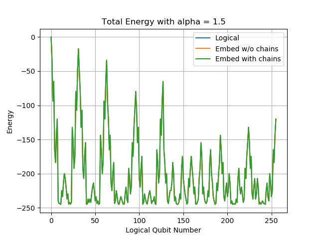
Figure 9: Gray Projection of Energy vs State for Test 1(i)

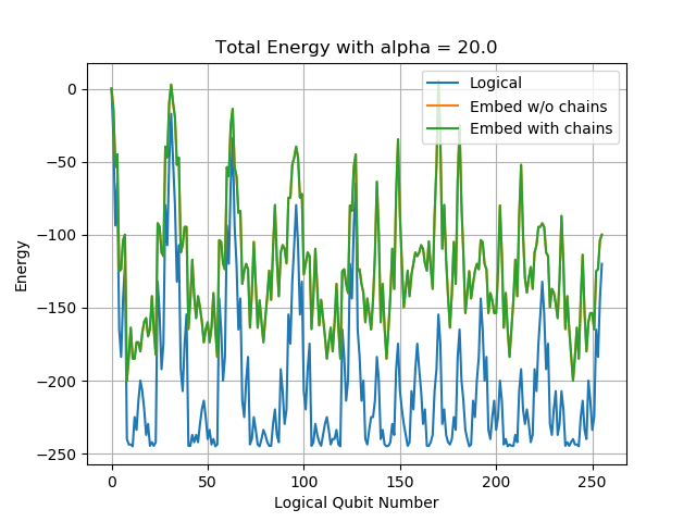
Figure 10: Gray Projection of Energy vs State for Test 1(i) without Weighted Counter-terms

Figure 11: Gray Projection of Energy vs State for Test 1(j)

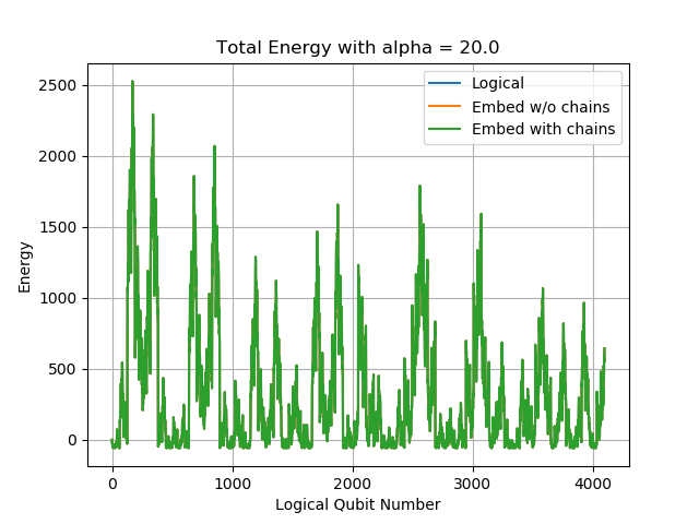
Figure 12: Gray Projection of Energy vs State for Test 2(f)

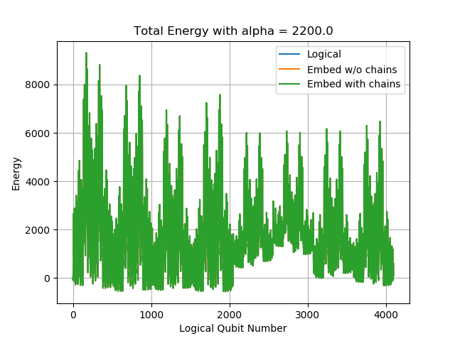
Figure 13: Gray Projection of Energy vs State for Test 2(g)

The $3\times 3$ ill-conditioned matrix was much more problematic. This is partly because of the nature of this test matrix, which is very nearly singular with an approximate $2$ dimensional kernel space. The energy spectrum of the ill-condition problem is given in Figure 12, and the energy spectrum of the pre-conditoned version is given in Figure 13. Although the pre-conditioned version is significantly better, it still required a very large chaining penalty, and even with that, it required thousands of “reads” (annealing runs) to reliably obtain the correct answer. In this case, it required sampling the state space with as many as $2500$ or more “reads” with $20\mu s$ anneal times. Only several orders of magnitude longer anneal times began to allow for a smaller number of reads. Here there were $2^{12}=4096$ final states for the logical Hamiltonian, so we were actually sampling with more than half as many distinct runs as the number of possible states. However, the $K_{12}$ embedding used for these runs had $56$ qubits. Therefore, the total state space for all qubits in the embedding was of size $2^{56}\approx 7\times 10^{16}$, so perhaps this large sampling requirement is not as bad as it may at first appear. Still, it is clear that there are still far too many excited states too close to the ground state and that the system is far from perfectly adiabatic here. However, it should be noted that the pre-conditioning still improved things somewhat, because we could not get the correct answer with even $10000$ “reads” for the original ill-conditioned problems.

The pre-conditioning method we used was very crude, rather ad-hoc, and ill-suited to practical matrix inversion problems for classical algorithms, but the intent was simply to test the effects of a simple pre-conditioning on the quantum annealing solutions. We have been studying this issue and believe it may be possible to pre-condition the problems better for solving these problems on a quantum annealing machine. In fact, we suspect that methods related to this approach may allow other QUBO problems suffering from similar pathologies to be “pre-conditioned” in way that better separates the ground state energy and allows more practical solutions on the annealer. This, however, is still work in progress, and we plan to further develop and test those ideas in the near future.

Appendix A Matrix Test Problems

The problems we solved to test our quantum annealing algorithm to solve equation (36) are listed below. Note that, although the QUBO $B_{ij}$ matrix is symmetric by construction, the matrix $M$ need not be symmetric.

1. Test Problems with $2\times 2$ Matrices

   1. Test $1(a)$:

      $$\bm{M}=\left(\begin{array}[]{cc}0.5&1.5\\ 1.5&0.5\end{array}\right), \mathbf{Y}=\left(\begin{array}[]{c}1.0\\ 0.0\end{array}\right), \mathbf{x}=\left(\begin{array}[]{c}-0.25\\ 0.75\end{array}\right)$$ (88)

   2. Test $1(b)$:

      $$\bm{M}=\left(\begin{array}[]{cc}0.5&1.5\\ 1.5&0.5\end{array}\right), \mathbf{Y}=\left(\begin{array}[]{c}0.0\\ 1.0\end{array}\right), \mathbf{x}=\left(\begin{array}[]{c}0.75\\ -0.25\end{array}\right)$$ (95)

   3. Test $1(c)$:

      $$\bm{M}=\left(\begin{array}[]{cc}2.0&-1.0\\ -0.5&0.5\end{array}\right), \mathbf{Y}=\left(\begin{array}[]{c}1.0\\ 0.0\end{array}\right), \mathbf{x}=\left(\begin{array}[]{c}1.0\\ 1.0\end{array}\right)$$ (102)

   4. Test $1(d)$:

      $$\bm{M}=\left(\begin{array}[]{cc}1.0&2.0\\ 0.5&0.5\end{array}\right), \mathbf{Y}=\left(\begin{array}[]{c}1.0\\ 0.0\end{array}\right), \mathbf{x}=\left(\begin{array}[]{c}-1.0\\ 1.0\end{array}\right)$$ (109)

   5. Test $1(e)$:

      $$\bm{M}=\left(\begin{array}[]{cc}3.0&2.0\\ 2.0&1.0\end{array}\right), \mathbf{Y}=\left(\begin{array}[]{c}1.0\\ 1.0\end{array}\right), \mathbf{x}=\left(\begin{array}[]{c}1.0\\ -1.0\end{array}\right)$$ (116)

   6. Test $1(f)$:

      $$\bm{M}=\left(\begin{array}[]{cc}1.0&0.5\\ 1.0&-0.5\end{array}\right), \mathbf{Y}=\left(\begin{array}[]{c}1.0\\ 1.0\end{array}\right), \mathbf{x}=\left(\begin{array}[]{c}1.0\\ 0.0\end{array}\right)$$ (123)

   7. Test $1(g)$:

      $$\bm{M}=\left(\begin{array}[]{cc}0.0&-2.0\\ -2.0&-1.5\end{array}\right), \mathbf{Y}=\left(\begin{array}[]{c}1.0\\ 0.25\end{array}\right), \mathbf{x}=\left(\begin{array}[]{c}0.25\\ -0.5\end{array}\right)$$ (130)

   8. Test $1(h)$:

      $$\bm{M}=\left(\begin{array}[]{cc}0.0&-2.0\\ -2.0&-1.5\end{array}\right), \mathbf{Y}=\left(\begin{array}[]{c}-0.5\\ -0.875\end{array}\right), \mathbf{x}=\left(\begin{array}[]{c}0.25\\ 0.25\end{array}\right)$$ (137)

   9. Test $1(i)$: Ill-conditioned problem with $\kappa\approx 25$

      $$\bm{M}=\left(\begin{array}[]{cc}1.0&2.0\\ 2.0&3.999\end{array}\right), \mathbf{Y}=\left(\begin{array}[]{c}4.0\\ 7.999\end{array}\right), \mathbf{x}=\left(\begin{array}[]{c}2.0\\ 1.0\end{array}\right)$$ (144)

   10. Test $1(j)$: Pre-conditioned version of $1(i)$ with $\kappa=5.0$

       $$\bm{M}=\left(\begin{array}[]{cc}1.80026&1.6019\\ 1.6019&4.19974\end{array}\right), \mathbf{Y}=\left(\begin{array}[]{c}5.2007\\ 7.40013\end{array}\right), \mathbf{x}=\left(\begin{array}[]{c}2.0\\ 1.0\end{array}\right)$$ (151)

2. Matrix Problems with $3\times 3$ Matrices

   1. Test $2(a)$:

      $$\bm{M}=\left(\begin{array}[]{ccc}0.0&-2.0&0.0\\ -2.0&1.5&0.0\\ 0.0&0.0&1.0\end{array}\right), \mathbf{Y}=\left(\begin{array}[]{c}1.0\\ 0.25\\ 1.0\end{array}\right), \mathbf{x}=\left(\begin{array}[]{c}0.25\\ -0.5\\ 1.0\end{array}\right)$$ (161)

   2. Test $2(b)$:

      $$\bm{M}=\left(\begin{array}[]{ccc}0.0&-2.0&0.0\\ -2.0&1.5&0.0\\ 0.0&0.0&1.0\end{array}\right), \mathbf{Y}=\left(\begin{array}[]{c}1.0\\ 0.25\\ 0.0\end{array}\right), \mathbf{x}=\left(\begin{array}[]{c}0.25\\ -0.5\\ 0.0\end{array}\right)$$ (171)

   3. Test $2(c)$:

      $$\bm{M}=\left(\begin{array}[]{ccc}1.0&0.0&0.0\\ 0.0&0.0&-2.0\\ 0.0&-2.0&-1.5\end{array}\right), \mathbf{Y}=\left(\begin{array}[]{c}1.0\\ 0.0\\ 0.25\end{array}\right), \mathbf{x}=\left(\begin{array}[]{c}0.25\\ 0.0\\ -0.5\end{array}\right)$$ (181)

   4. Test $2(d)$:

      $$\bm{M}=\left(\begin{array}[]{ccc}1.0&0.0&0.0\\ 0.0&0.0&-2.0\\ 0.0&-2.0&-1.5\end{array}\right), \mathbf{Y}=\left(\begin{array}[]{c}1.0\\ 1.0\\ 0.25\end{array}\right), \mathbf{x}=\left(\begin{array}[]{c}1.0\\ 0.25\\ -0.5\end{array}\right)$$ (191)

   5. Test $2(e)$:

      $$\bm{M}=\left(\begin{array}[]{ccc}1.0&0.0&0.0\\ 0.0&0.0&-2.0\\ 0.0&-2.0&-1.5\end{array}\right), \mathbf{Y}=\left(\begin{array}[]{c}0.0\\ 1.0\\ 0.25\end{array}\right), \mathbf{x}=\left(\begin{array}[]{c}0.0\\ 0.25\\ -0.5\end{array}\right)$$ (201)

   6. Test $2(f)$: Ill-conditioned problem with $\kappa\approx 78$

      $$\bm{M}=\left(\begin{array}[]{ccc}-4.0&6.0&1.0\\ 8.0&-11.0&-2.0\\ -3.0&4.0&1.0\end{array}\right), \mathbf{Y}=\left(\begin{array}[]{c}0.75\\ -1.25\\ 0.25\end{array}\right), \mathbf{x}=\left(\begin{array}[]{c}0.0\\ 0.25\\ -0.75\end{array}\right)$$ (211)

   7. Test $2(g)$: Pre-conditioned version $2(g)$ with $\kappa\approx 1$

      $$\bm{M}=\left(\begin{array}[]{ccc}6.1795&11.8207&2.0583\\ 15.673&-7.56717&-3.8520\\ -5.6457&7.96872&15.9418\end{array}\right), \mathbf{Y}=\left(\begin{array}[]{c}1.4114\\ 0.9972\\ 9.9643\end{array}\right), \mathbf{x}=\left(\begin{array}[]{c}0.0\\ 0.25\\ -0.75\end{array}\right)$$ (221)

- (1) A. Harrow, A. Hassidim, and S. Lloyd, Phys. Rev. Lett. 103, 150502 (2009).
- (2) Stefanie Barz, Ivan Kassal, Martin Ringbauer, Yannick Ole Lipp, Borivoje Dakic ̵́, Ala ̵́n Aspuru-Guzik, Philip Walther, Solving systems of linear equations on a quantum computer, arXiv:1302.1210v1 (2013).
- (3) Stefanie Barz, Ivan Kassal, Martin Ringbauer, Yannick Ole Lipp, Borivoje Dakic ̵́, Ala ̵́n Aspuru-Guzik, Philip Walther, Solving systems of linear equations on a quantum computer, arXiv:1302.1946v1 (2013).
- (4) X.-D. Cai, C. Weedbrook, Z.-E. Su, M.-C. Chen, Mile Gu, M.-J. Zhu, Li Li, Nai-Le Liu, Chao-Yang Lu, Jian-Wei Pan, Experimental quantum computing to solve systems of linear equations, arXiv:1302.4310v2 (2013).
- (5) Edward Farhi, Jeffrey Goldstone, Sam Gutmann and Michael Sipser, Quantum Computation by Adiabatic Evolution, arXive:000110 (2000).
- (6) E. Ising, Z. Phys. 31 (1925) 253.
- (7) Press, William H.; Teukolsky, Saul A.; Vetterling, William T.; Flannery, Brian P. ”Section 22.3. Gray Codes”. Numerical Recipes: The Art of Scientific Computing (3rd ed.), New York, USA: Cambridge University Press. ISBN 978-0-521-88068-8 (2007).
- (8) Messiah, Albert “Chapter XVII.” Quantum Mechanics. Dover Publications. ISBN 0-486-40924-4. (1999)