Deep Learning of truncated singular values for limited view photoacoustic tomography

Abstract

We develop a data-driven regularization method for the severely ill-posed problem of photoacoustic image reconstruction from limited view data. Our approach is based on the regularizing networks that have been recently introduced and analyzed in [J. Schwab, S. Antholzer, and M. Haltmeier. Big in Japan: Regularizing networks for solving inverse problems (2018), arXiv:1812.00965] and consists of two steps. In the first step, an intermediate reconstruction is performed by applying truncated singular value decomposition (SVD). In order to prevent noise amplification, only coefficients corresponding to sufficiently large singular values are used, whereas the remaining coefficients are set zero. In a second step, a trained deep neural network is applied to recover the truncated SVD coefficients. Numerical results are presented demonstrating that the proposed data driven estimation of the truncated singular values significantly improves the pure truncated SVD reconstruction. We point out that proposed reconstruction framework can straightforwardly be applied to other inverse problems, where the SVD is either known analytically or can be computed numerically.

Keywords: Photoacoustic tomography, image reconstruction, deep learning, nullspace learning, singular value decomposition, neural networks.

1 Introduction

Recently, a considerable amount of research has been done on the use of deep neural networks for various image reconstruction tasks. Deep convolutional neural networks (CNNs) have shown excellent results for deconvolution, inpainting or denoising problems. They have also been successfully used in tomographic reconstruction problems, like full waveform inversion, x-ray tomography, magnetic resonance imaging and photoacoustic tomography (see, for example [1, 2, 3, 4, 5, 6, 7, 8]). There exist several different deep learning approaches to solve inverse problems. This includes CNNs in iterative schemes [5, 6, 1], or using a single CNN to improve an initial reconstruction [4, 9, 10]. Very recently, we have proven that sequences of suitable neural networks in combination with classical regularizations lead to convergent regularization methods [11]. In the present paper, we apply the concept of regularizing networks to the limited view problem of photoacoustic tomography (PAT). In particular, we use truncated SVD as initial regularization method for approximating a low frequency approximation of the photoacoustic (PA) source. In the second step, a deep network is trained to recover the missing high frequency part.

PAT is a tomographic imaging method based on the generation of acoustic waves induced by pulsed optical illumination (see Figure 1). The induced pressure waves are measured outside of the investigated sample and used for reconstructing the PA source. In many practical applications, the pressure data cannot be measured on a surface fully surrounding the sample, which makes the reconstruction problem severely ill-posed. This implies that exact inversion methods are unstable and significantly amplify noise. Therefore, one has to apply regularization techniques which replace the exact inverse (or pseudo-inverse) by approximate but stable inversion methods. In this paper, we work with a fully discretized model based approach, where we recover the expansion coefficients of the PA source with respect to certain basis functions [12, 13, 14, 15, 16, 17]. The discretized limited view scenario yields to the solution of a severely ill-conditioned system of linear equations. The ill-conditioning is reflected by the fact that the singular values decay rapidly and a large fraction of them is close to zero.

In order to solve the discrete ill-conditioned limited view problem of PAT, we propose the following deep-learning based reconstruction procedure. In a first step, we apply truncated SVD to obtain an intermediate reconstruction formed by the singular components corresponding to sufficiently large singular values. By truncating the small singular values we prevent the reconstruction to amplify noise since small singular values of the forward matrix correspond to large singular values of the inverse matrix that amplify noise. For recovering the truncated singular components, in a second step, we train a deep CNN that maps the intermediate reconstruction to the truncated part. The actual reconstruction is the sum of the intermediate reconstruction and the residual image found by the network. Opposed to strict null-space learning proposed in [10], not only the part in the kernel of the operator (corresponding to singular value zero) is learned, but also parts corresponding to small singular values. Consequently, the approach proposed here can be seen as approximate null-space learning. Our numerical results demonstrate, that the proposed deep learning based extension of truncated singular components significantly improves pure truncated SVD.

Figure 1: Basic principles of PAT. The absorption of short optical pulses inside a semitransparent sample causes thermoelastic expansion, which in turn induces acoustic pressure waves. The acoustic waves propagate outwards, where they are measured and used to reconstruct an image of the interior.

2 Photoacoustic tomography

2.1 Continuous model

Throughout this paper we work with homogeneous medium and describe the acoustic wave propagation in PAT by the initial value problem

$$\partial_{t}^{2}p(\mathbf{r},t)-c^{2}\Delta_{\mathbf{r}}p(\mathbf{r},t) =0\,,$$

$$p(\mathbf{r},0) =f(\mathbf{r})\,,$$ (1)

$$\partial_{t}p(\mathbf{r},0) =0\,.$$

Here $d=2$ or $d=3$ is the spatial dimension, $f\colon\mathbb{R}^{d}\to\mathbb{R}$ the PA source, $\mathbf{r}\in\mathbb{R}^{d}$ the spatial variable, $t\in\mathbb{R}$ the time variable, $\Delta_{\mathbf{r}}$ the spatial Laplacian, and $c$ is the constant speed of sound. We assume that the PA exists inside the region $R\subset\mathbb{R}^{d}$. After temporal rescaling, in the following we assume normalized speed of sound $c=1$. The inverse problem of PAT consists in reconstructing $f$ from values of $p(\mathbf{s},t)$ for points $\mathbf{s}\in S$ on a measurement surface $S\subset\partial R$ and times $t\geq 0$. For point-like detectors, the spatial dimension $d=3$ is relevant. In this work, we consider the case $d=2$, which is relevant for PAT using integrating line detectors [18, 19]. Using integrating line detectors leads to a set of 2D problems ((1) for $d=2$), where the initial PA source corresponds to the projection of the 3D source in a certain direction. By varying the projection direction and applying the inverse Radon transform to the projection images one can reconstruct the 3D source, although the projection images are already of diagnostic value.

We denote by $\mathcal{A}$ the operator, that maps a PA source $f$ to the solution $\mathcal{A}f\colon\partial R\times[0,\infty)\rightarrow\mathbb{R}$ restricted to $\partial R$. In the full data situation, the goal is to reconstruct $f$ from noisy versions of $\mathcal{A}f$. This problem can be solved stably by means of explicit inversion formulas known for certain geometries [18, 20, 21, 22, 23, 24, 25, 26]. In practical applications, measurement data are only available on a surface $S\subsetneq\partial R$ that does not fully enclose the investigated sample. In this case, the inverse problem of PAT becomes severely ill-posed. [27, 28, 29, 30] In this work we consider the limited view problem in a discrete setting as described in the following subsection.

2.2 Discretization

For the discretization we assume that the initial pressure has the following form

$$f(\mathbf{r})=\sum_{i=1}^{N^{2}}x_{i}\,\varphi_{i}(\mathbf{r})\quad\text{ for expansion coefficients $x_{i}\in\mathbb{R}$}\,.$$ (2)

Here $\varphi_{i}(\mathbf{r})=\varphi(\mathbf{r}-\mathbf{r}_{i})$ are translated version of a fixed basis function $\varphi\colon\mathbb{R}^{2}\rightarrow\mathbb{R}$, where the centers $\mathbf{r}_{i}$ are arranged on a Cartesian grid. In particular, we consider so-called Kaiser-Bessel functions which are radially symmetric functions of compact support that are very popular for tomographic inverse problems [31, 32, 17]. The generalized Kaiser-Bessel functions depend on three parameters and are defined by

$$\varphi(\mathbf{r})\triangleq\begin{cases}\left(\sqrt{1-{\left\|\mathbf{r}\right\|}^{2}/a^{2}}\right)^{m}\frac{I_{m}\left(\gamma\sqrt{1-{\left\|\mathbf{r}\right\|}^{2}/a^{2}}\right)}{I_{m}(\gamma)}\quad&\text{ for }{\left\|\mathbf{r}\right\|}\geq a\\ 0\quad&\text{ else}\,.\end{cases}$$

Here $I_{m}$ is the modified Bessel function of the first kind of order $m\in\mathbb{N}$, $\gamma>0$ the window taper and $a$ the radius of the support. Since the forward operator $\mathcal{A}$ is linear we have $\mathcal{A}f=\sum_{i=1}^{N^{2}}x_{i}\mathcal{A}\varphi_{i}$.

In applications, the number of spatial and temporal measurements is finite. We assume that measurements are made with sampling points $(\mathbf{s}_{n})_{n=1}^{N_{s}}$ on the detection surface $S$ and temporal sampling points $(t_{j})_{j=1}^{N_{t}}$ in $[0,T]$. In our experiments presented below, we consider equidistant spatial sampling points $\mathbf{s}_{n}=(\cos(n\pi/N_{s}),\sin(n\pi/N_{s}))$ for $n=1,\ldots,N_{s}$ and equidistant temporal sampling points $t_{j}=jT/N_{t}$ for $j=1,\ldots,N_{t}$. For each basis function $\varphi_{i}$, we write the corresponding data $\mathcal{A}\varphi_{i}$ evaluated at the discretization points into the columns of a matrix, $\mathbf{A}_{N_{t}(n-1)+j,i}\triangleq\mathcal{A}\varphi_{i}(\mathbf{s}_{n},t_{j})$. This results in a linear system of equations for the expansions coefficients of the PA source:

$$\text{Recover $x\in\mathbb{R}^{N^{2}}$ from data }\quad y=\mathbf{A}x+\xi\,.$$ (3)

Here $\mathbf{A}\in\mathbb{R}^{N_{t}N_{s}\times N^{2}}$ is the system matrix, $\xi$ models the error in the data, and $y\in\mathbb{R}^{N_{t}N_{s}}$ is vector of the noisy data $y_{N_{t}(n-1)+j}=\mathcal{A}f(\mathbf{s}_{n},t_{j})+\xi_{N_{t}(n-1)+j,i}$ given on the measurement points. Equation (3) is ill-conditioned, reflecting the ill-posedness of the underlying continuous limited view problem.

In the following, we consider the fully discrete problem of recovering the vector $x$ of expansion coefficients in (3). The PA source can then be recovered by evaluating the expansion (2). Recall that $\varphi_{i}$ are translated versions of a fixed basis function with centers on a Cartesian grid. We therefore can arrange the entries of a vector $x\in\mathbb{R}^{N^{2}}$ as $N\times N$ image in a natural manner. This image representation will be used when visualizing elements in $\mathbb{R}^{N^{2}}$ and for applying the CNNs.

3 Deep learning of singular value expansion

In this section we describe the proposed deep learning method for solving the discrete linear system (3). As it is shown in [11] the combination of a classical regularization method with deep CNNs yields a regularization method together with quantitative error estimates. Here we use the truncated SVD decomposition as classical regularization method and combine it with a deep network that recovers the truncated coefficients.

3.1 Truncated SVD reconstruction

In the following, let $\mathbf{A}=\mathbf{U}\mathbf{\Sigma}\mathbf{V}^{\mathsf{T}}$ denote the singular value decomposition of the forward matrix $\mathbf{A}$. Here $\mathbf{U}\in\mathbb{R}^{N_{t}N_{s}\times N_{t}N_{s}}$ and $\mathbf{V}\in\mathbb{R}^{N^{2}\times N^{2}}$ are orthogonal matrices, and $\mathbf{\Sigma}\in\mathbb{R}^{N_{t}N_{s}\times N}$ is the diagonal matrix. The tuples of columns $(u_{i})_{i=1}^{N_{t}N_{s}}$ and $(v_{i})_{i=1}^{N^{2}}$ are orthonormal systems in $\mathbb{R}^{N_{t}N_{s}}$ and $\mathbb{R}^{N^{2}}$, respectively. The diagonal entries $\sigma_{1}\geq\sigma_{2}\geq\cdots\geq\sigma_{\min\{N_{t}N_{s},N^{2}\}}\geq 0$ of $\mathbf{\Sigma}$ are the singular values of $\mathbf{A}$. The number $r\leq\min\{N_{t}N_{s},N^{2}\}$ of non-vanishing singular values equals the rank of the matrix $\mathbf{A}$. Using the SVD, we have the explicit formulas for the forward matrix $\mathbf{A}$ and its Moore-Penrose pseudo-inverse $\mathbf{A}^{\boldsymbol{\texttt{+}}}$ (also called Moore-Penrose inverse),

$$\mathbf{A}x =\sum_{i=1}^{r}\sigma_{i}\left\langle u_{i},x\right\rangle v_{i}\quad\text{ for }x\in\mathbb{R}^{N^{2}}$$ (4)

$$\mathbf{A}^{\boldsymbol{\texttt{+}}}y=\mathbf{V}\mathbf{\Sigma}^{\boldsymbol{\texttt{+}}}\mathbf{U}^{\mathsf{T}}y =\sum_{i=1}^{r}\frac{1}{\sigma_{i}}\left\langle y,v_{i}\right\rangle u_{i}\quad\text{ for }y\in\mathbb{R}^{N_{t}N_{s}}\,.$$ (5)

In particular, for exact data $y=\mathbf{A}x$, (5) gives an explicit solution for the discrete limited view PAT problem (3). In the case of noisy data $y=\mathbf{A}x+\xi$, the small singular values $\sigma_{i}$ cause severe amplification of the noise coefficients $\left\langle\xi,v_{i}\right\rangle$ and typically yields to useless reconstruction results. To stabilize the inversion problem one has to apply regularization methods which replace the exact pseudo-inverse by a stable approximate inverse.

In this paper, we work with truncated SVD which is a well established regularization method. Truncated SVD consists of a family $(\mathbf{B}_{\alpha})_{\alpha>0}$ of approximations of the pseudo-inverse defined by

$$\mathbf{B}_{\alpha}(y)=\sum_{\sigma_{i}^{2}\geq\alpha}\frac{1}{\sigma_{i}}\left\langle y,v_{i}\right\rangle u_{i}\quad\text{for }y\in\mathbb{R}^{N_{t}N_{s}}.$$ (6)

Applying truncated SVD with regularization parameter $\alpha>0$ (which is chosen depending on the noise level) prevents amplification of measurement errors. In particular, when applied to noisy data satisfying ${\left\|\mathbf{A}x-y\right\|}\leq\delta$ for some noise level $\delta>0$, it satisfies the stability estimate ${\left\|\mathbf{B}_{\alpha}y-\mathbf{A}^{\boldsymbol{\texttt{+}}}\mathbf{A}x\right\|}\leq\delta/\sqrt{\alpha}+{\left\|(\mathbf{A}^{\boldsymbol{\texttt{+}}}-\mathbf{B}_{\alpha})\mathbf{A}x\right\|}$. This implies convergence of truncated SVD in the case that the regularization parameter $\alpha=\alpha(\delta)$ is chosen such that $\alpha\to 0$ and $\delta^{2}/\alpha\to 0$ as $\delta\to 0$. Quantitative error estimates require bounding the approximation term ${\left\|(\mathbf{A}^{\boldsymbol{\texttt{+}}}-\mathbf{B}_{\alpha})\mathbf{A}x\right\|}$. Noting that $(\mathbf{A}^{\boldsymbol{\texttt{+}}}-\mathbf{B}_{\alpha})\mathbf{A}x=\sum_{\sigma_{i}^{2}<\alpha}\left\langle x,u_{i}\right\rangle u_{i}$ this requires $x$ being smooth in the sense that the contribution of coefficients corresponding to small singular values is small.

3.2 Deep Learning of truncated singular values

According to (6), the truncated SVD approximates coefficients $\left\langle x,u_{i}\right\rangle$ corresponding to singular values with $\sigma_{i}^{2}\geq\alpha$. Coefficients corresponding to smaller singular values are set to zero. To improve the reconstruction we propose to train a CNN that reconstructs the missing part $x-\mathbf{B}_{\alpha}\mathbf{A}x=\sum_{\sigma_{i}^{2}<\alpha}\left\langle x,u_{i}\right\rangle u_{i}$ from the estimated part $\mathbf{B}_{\alpha}y\simeq\mathbf{B}_{\alpha}\mathbf{A}x$. Adding nonzero values to the truncated singular value components allows to better approximate non-smooth elements. To achieve a deep learning based expansion of singular values, we consider a family of regularizing networks $(\mathbf{R}_{\alpha})_{\alpha>0}$ of the form

$$\mathbf{R}_{\alpha}(y)\triangleq\sum_{\sigma_{i}^{2}\geq\alpha}\frac{1}{\sigma_{i}}\left\langle y,v_{i}\right\rangle u_{i}+{\mathbf{\Phi}}_{\alpha}\left(\sum_{\sigma_{i}^{2}\geq\alpha}\frac{1}{\sigma_{i}}\left\langle y,v_{i}\right\rangle u_{i}\right)\;\text{ with }{\mathbf{\Phi}}_{\alpha}(z)\triangleq\sum_{\sigma_{i}^{2}<\alpha}\left\langle\mathbf{U}_{\alpha}z,u_{i}\right\rangle u_{i}\,.$$ (7)

Here $\sum_{\sigma_{i}^{2}\geq\alpha}{1}/{\sigma_{i}}\left\langle y,v_{i}\right\rangle u_{i}=\mathbf{B}_{\alpha}y$ is the truncated SVD reconstruction, $\mathbf{U}_{\alpha}\colon\mathbb{R}^{N^{2}}\to\mathbb{R}^{N^{2}}$ a CNN that operates on elements in $\mathbb{R}^{N^{2}}$ as $N\times N$ images, and $\alpha$ is the regularization parameter.

Using the projected network ${\mathbf{\Phi}}_{\alpha}$ instead of the original network $\mathbf{U}_{\alpha}$ implies that the non-vanishing coefficients of the truncated SVD expansion are unaffected by the network. As a consequence, $\mathbf{B}_{\alpha}$ and $\mathbf{R}_{\alpha}$ reconstruct the same low frequency part $\sum_{\sigma_{i}^{2}\geq\alpha}\frac{1}{\sigma_{i}}\left\langle y,v_{i}\right\rangle u_{i}$. The subsequent application of the network $\Phi_{\alpha}$ adds high frequency components that are missing in the truncated SVD reconstruction. In particular, ${\mathbf{\Phi}}_{\alpha}$ is a deep CNN with $\operatorname{ran}({\mathbf{\Phi}}_{\alpha})\subset\operatorname{span}\{u_{i}\mid\sigma_{i}^{2}<\alpha\}$ which results in a data driven continuation of the truncated SVD. The CNNs ${\mathbf{\Phi}}_{\alpha}$ are trained to map the truncated SVD reconstruction $\mathbf{B}_{\alpha}(y)$ lying in the space spanned by the reliable basis elements (corresponding to large enough singular values of the operator $\mathbf{A}$) to the coefficients of the unreliable basis elements (corresponding to small singular values). Details on the selection of the regularization parameter, the used network architecture, and the network training will be discussed in Section 4.

4 Numerical results

4.1 Discretization

To evaluate the regularization method described in Section 3, we use a discretization of PA sources using $128\times 128$ translated Kaiser-Bessel basis functions $\varphi_{i}(\mathbf{r})=\varphi(\mathbf{r}-\mathbf{r}_{i})$ with center points $\mathbf{r}_{i}=(-1,1)+2(i_{1}-1,i_{2}-1)/127$ for $i_{1},i_{2}=1,\dots,128$. We have chosen support radius $a=0.055$, window taper $\gamma=7$ and smoothness parameter $m=2$. We consider measurement on a semi circle with radius 1, see Figure 2. We use a total number of $N_{s}=400$ detector positions and $N_{t}=376$ equidistant measurements in time in the interval $[0,3.75]$, leading to a system matrix of size $\mathbf{A}\in\mathbb{R}^{150400\times 16384}$.

The entries of the system matrix $\mathbf{A}$ have been constructed by computing the solution of the initial value problem for the basis function $\varphi$ centered at $0$ for different detector-source distances. For that purpose we evaluated solution formula

$$p(r,t)\triangleq\frac{1}{2\pi}\frac{\partial}{\partial t}\int_{0}^{t}\int_{\partial B_{1}(0)}\frac{r\varphi(\mathbf{s}+r\omega)}{\sqrt{t^{2}-r^{2}}}\ \mathrm{d}\omega\ \mathrm{d}r\,,$$

for varying $r={\left\|\mathbf{s}\right\|}$. Using that solution of the wave equation with initial data $\varphi_{i}(\mathbf{r})=\varphi(\mathbf{r}-\mathbf{r}_{i})$ evaluated at $\mathbf{s}$ equals $p(\mathbf{s}-\mathbf{r}_{i},t)$, the entries $\mathbf{A}\varphi_{i}$ have been computed numerically by using linear interpolation. The limited view scenario results in a severely ill-posed reconstruction problem (3).

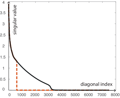
Figure 2: Considered limited view measurement geometry. Left: The phantom is allowed to take non-vanishing values in the square $[-1,1]$. Measurements are made on a semi circle of radius one, resulting in a severally ill-posed reconstruction problem. Right: solid black curve shows the singular values of the corresponding discrete system matrix using $16384$ basis functions and $150400$ data points. A large fraction of the singular values is zero or close to zero, reflecting the ill-posedness. The red dashed curve indicates the used singular values for $7\text{\,}\mathrm{\char 37\relax}$ additive Gaussian noise.

4.2 Network design

For image reconstruction, we use the reconstruction network (7), which can be written in the form $\mathbf{R}_{\alpha}=(\operatorname{Id}+\mathbf{P}_{\alpha}\mathbf{U}_{\alpha})\mathbf{B}_{\alpha}$. Here $\mathbf{B}_{\alpha}$ is the truncated SVD, $\mathbf{U}_{\alpha}\colon\mathbb{R}^{N^{2}}\to\mathbb{R}^{N^{2}}$ a trained deep neural network, and $\mathbf{P}_{\alpha}$ the projection onto the space $\operatorname{span}\{u_{i}\mid\sigma_{i}^{2}<\alpha\}$ spanned by the truncated singular vectors. To choose the regularization parameter $\alpha$ we use the following empirical approach. We compute noise-free data $\mathbf{A}x$ and noisy data $y=\mathbf{A}x+\xi$, respectively, for different PA sources and different realizations of additive Gaussian noise. Then we evaluate the truncated SVD reconstructions $\mathbf{B}_{\alpha}y$ for different regularization parameters and empirically chose such a regularization parameter, where $\mathbf{B}_{\alpha}\mathbf{A}x$ is close to $is\mathbf{B}_{\alpha}y$ is small. As shown in the right image in Figure 2, for additive Gaussian noise with a standard deviation equals $7\text{\,}\mathrm{\char 37\relax}$ of the maximum of $\mathbf{A}x$, this results in a regularization parameter where the first 604 singular values are kept.

To train the networks $\mathbf{R}_{\alpha}$ we generated $N_{\rm train}=3500$ training pairs $(y_{n},x_{n})_{n=1}^{N_{\rm train}}$ where $x_{n}$ are training phantoms and $y_{n}=\mathbf{A}x_{n}$ the corresponding exact data. The phantoms $x_{n}$ consist of randomly modified Shepp-Logan phantoms, where the position, size and orientation of the objects are randomly chosen and additionally some finer structures are added. Furthermore, a randomly generated deformation was applied to the Shepp-Logan like phantoms. Training was performed end-to-end using noise-free data $\mathbf{A}x_{n}=y_{n}$ by minimizing the error functional

$$E_{\alpha}(\mathbf{U}_{\alpha})=\frac{1}{N_{\rm train}}\sum_{n=1}^{N_{\rm train}}{\left\|x_{n}-(\operatorname{Id}+\mathbf{P}_{\alpha}\mathbf{U}_{\alpha})\mathbf{B}_{\alpha}\mathbf{A}x_{n}\right\|}_{2}^{2}\,,$$

over all free parameters in $\mathbf{U}_{\alpha}$. In all cases, the network was trained for 70 epochs using stochastic gradient descent with a learning rate of 0.01 and a momentum parameter 0.99. In our results we use the U-net architecture [33] for $\mathbf{U}_{\alpha}$; however our approach can also be combined with different CNN architectures.

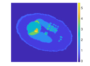
(a)

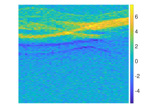
(b)

Figure 3: Phantom and noisy data. Left: Test phantom generated by the method described above not contained in the training set. Right: Limited view data with $7\text{\,}\mathrm{\char 37\relax}$ additive Gaussian noise.

4.3 Reconstruction results

Figure 3 (left) shows a randomly chosen modified Shepp-Logan type phantom $x$. The phantom is different from all training phantoms but generated using the same random model. The corresponding data obtained by multiplying $x$ with the system matrix and adding Gaussian noise with a standard deviation of $7\text{\,}\mathrm{\char 37\relax}$ of the maximum of $\mathbf{A}x$ is shown in Figure 3, right. Figure 4 (right column) shows the reconstruction with the proposed regularization network. The intermediate truncated SVD reconstruction $\mathbf{B}_{\alpha}y$ used as input for the network $(\operatorname{Id}+\mathbf{P}_{\alpha}\mathbf{U}_{\alpha})$ is shown in the second column. For comparison purpose, in the left column in Figure 4 we show the optimal truncated SVD reconstruction, where the regularization parameter is chosen in such a way, that $\mathbf{B}_{\alpha}y$ has the minimal $\ell^{2}$-difference to the ground truth image.

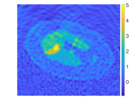
(a)

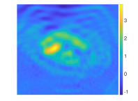
(b)

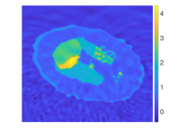
(c)

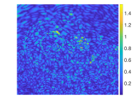
(d)

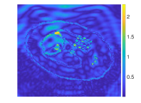
(e)

(f)

Figure 4: Reconstructions result for $7\text{\,}\mathrm{\char 37\relax}$ noise. Top row: Optimally truncated SVD (left), truncated SVD used as input to the CNN (center), and proposed CNN continuated SVD (right). Bottom row: Absolute differences from the ground truth corresponding to the reconstruction in the top row.

We observe, that the reconstructions with the proposed regularization method are visually superior to the reconstructions using truncated SVD with optimally chosen regularization parameter. Evaluation of the relative mean squared error $\frac{1}{500}\sum_{i=1}^{500}{\|\mathbf{R}_{\alpha}y_{i}-x_{i}\|_{2}}/{\|x_{i}\|_{2}}$ averaged over 500 examples with noisy data not contained in the training data set, yielded an average error of 0.0887, opposed to 0.1563 for the reconstructions coming from the optimal truncated SVD. Reconstruction results from data with $4\text{\,}\mathrm{\char 37\relax}$ additive Gaussian noise are shown in Figure 5. Again the proposed regularization network clearly outperforms the optimal truncated SVD reconstruction.

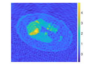
(a)

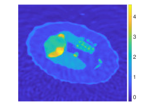
(b)

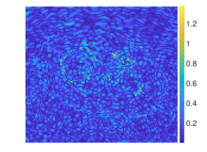
(c)

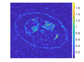
(d)

Figure 5: Reconstructions result for $4\text{\,}\mathrm{\char 37\relax}$ noise. Top row: Optimally truncated SVD (left), and proposed CNN continuated SVD (right). Bottom row: Absolute differences from the ground truth corresponding to the reconstruction in the top row.

5 Conclusion

In this paper we investigates the use of regularizing networks for the limited view problem of PAT. The truncated SVD is used to reconstruct an intermediate low resolution approximation, a subsequent projection network recovers the high frequency parts. The reconstruction networks are shown to significantly improve the truncated SVD as regularization method. Further work will be done to refine the network architecture, combine it with different regularization methods, compare it to other deep learning based regularization methods, and to evaluate various approaches on experimental data.

References

- [1] J. Adler and O. Öktem, “Solving ill-posed inverse problems using iterative deep neural networks,” Inverse Probl. 33(12), p. 124007, 2017.
- [2] S. Antholzer, M. Haltmeier, and J. Schwab, “Deep learning for photoacoustic tomography from sparse data,” Inverse Probl. Sci. Eng. , pp. 1–19, 2018.
- [3] T. A. Bubba, G. Kutyniok, M. Lassas, M. März, W. Samek, S. Siltanen, and V. Srinivasan, “Learning the invisible: A hybrid deep learning-shearlet framework for limited angle computed tomography,” 2018. arXiv:1811.04602.
- [4] Y. Han and J. C. Ye, “Framing u-net via deep convolutional framelets: Application to sparse-view CT,” IEEE Trans. Med. Imag. 37(6), pp. 1418–1429, 2018.
- [5] H. Gupta, K. H. Jin, H. Q. Nguyen, M. T. McCann, and M. Unser, “CNN-based projected gradient descent for consistent ct image reconstruction,” IEEE Trans. Med. Imag. 37(6), pp. 1440–1453, 2018.
- [6] E. Kobler, T. Klatzer, K. Hammernik, and T. Pock, “Variational networks: connecting variational methods and deep learning,” in German Conference on Pattern Recognition, pp. 281–293, Springer, 2017.
- [7] H. Li, J. Schwab, S. Antholzer, and M. Haltmeier, “NETT: Solving inverse problems with deep neural networks,” 2018. rXiv:1803.00092.
- [8] J. C. Ye, Y. Han, and E. Cha, “Deep convolutional framelets: A general deep learning framework for inverse problems,” SIAM J. Imaging Sci. 11(2), pp. 991–1048, 2018.
- [9] K. H. Jin, M. T. McCann, E. Froustey, and M. Unser, “Deep convolutional neural network for inverse problems in imaging,” IEEE Trans. Image Process. 26(9), pp. 4509–4522, 2017.
- [10] J. Schwab, S. Antholzer, and M. Haltmeier, “Deep null space learning for inverse problems: Convergence analysis and rates,” 2018.
- [11] J. Schwab, S. Antholzer, and M. Haltmeier, “Big in Japan: Regularizing networks for solving inverse problems,” 2018. arXiv:1812.00965.
- [12] X. L. Dean-Ben, A. Buehler, V. Ntziachristos, and D. Razansky, “Accurate model-based reconstruction algorithm for three-dimensional optoacoustic tomography,” IEEE Trans. Med. Imag. 31(10), pp. 1922–1928, 2012.
- [13] G. Paltauf, R. Nuster, M. Haltmeier, and P. Burgholzer, “Experimental evaluation of reconstruction algorithms for limited view photoacoustic tomography with line detectors,” Inverse Probl. 23(6), p. S81, 2007.
- [14] G. Paltauf, J. A. Viator, S. A. Prahl, and S. L. Jacques, “Iterative reconstruction algorithm for optoacoustic imaging,” J. Acoust. Soc. Am. 112(4), pp. 1536–1544, 2002.
- [15] A. Rosenthal, V. Ntziachristos, and D. Razansky, “Acoustic inversion in optoacoustic tomography: A review,” Curr. Med. Imaging Rev. 9(4), pp. 318–336, 2013.
- [16] J. Zhang, M. A. Anastasio, P. J. La Rivière, and L. V. Wang, “Effects of different imaging models on least-squares image reconstruction accuracy in photoacoustic tomography,” IEEE Trans. Med. Imag. 28(11), pp. 1781–1790, 2009.
- [17] J. Schwab, S. Pereverzyev Jr, and M. Haltmeier, “A Galerkin least squares approach for photoacoustic tomography,” SIAM J. Numer. Anal. 56(1), pp. 160–184, 2018.
- [18] P. Burgholzer, J. Bauer-Marschallinger, H. Grün, M. Haltmeier, and G. Paltauf, “Temporal back-projection algorithms for photoacoustic tomography with integrating line detectors,” Inverse Probl. 23(6), p. S65, 2007.
- [19] G. Paltauf, R. Nuster, M. Haltmeier, and P. Burgholzer, “Photoacoustic tomography using a Mach-Zehnder interferometer as an acoustic line detector,” Appl. Opt. 46(16), pp. 3352–3358, 2007.
- [20] L. A. Kunyansky, “Explicit inversion formulae for the spherical mean Radon transform,” Inverse Probl. 23(1), pp. 373–383, 2007.
- [21] D. Finch, M. Haltmeier, and Rakesh, “Inversion of spherical means and the wave equation in even dimensions,” SIAM J. Appl. Math. 68(2), pp. 392–412, 2007.
- [22] M. Xu and L. V. Wang, “Universal back-projection algorithm for photoacoustic computed tomography,” Phys. Rev. E 71, 2005.
- [23] D. Finch, S. K. Patch, and Rakesh, “Determining a function from its mean values over a family of spheres,” SIAM J. Math. Anal. 35(5), pp. 1213–1240, 2004.
- [24] M. Haltmeier, “Universal inversion formulas for recovering a function from spherical means,” SIAM J. Math. Anal. 46(1), pp. 214–232, 2014.
- [25] V. Palamodov, “Time reversal in photoacoustic tomography and levitation in a cavity,” Inverse Probl. 30(12), p. 125006, 2014.
- [26] L. V. Nguyen, “On a reconstruction formula for spherical radon transform: a microlocal analytic point of view,” Anal. Math. Phys. 4(3), pp. 199–220, 2014.
- [27] Y. Xu, L. V. Wang, G. Ambartsoumian, and P. Kuchment, “Reconstructions in limited-view thermoacoustic tomography,” Med. Phys. 31(4), pp. 724–733, 2004.
- [28] J. Frikel and E. T. Quinto, “Artifacts in incomplete data tomography with applications to photoacoustic tomography and sonar,” SIAM J. Appl. Math. 75(2), pp. 703–725, 2015.
- [29] L. L. Barannyk, J. Frikel, and L. V. Nguyen, “On artifacts in limited data spherical radon transform: curved observation surface,” Inverse Probl. 32(1), p. 015012, 2015.
- [30] P. Stefanov and G. Uhlmann, “Thermoacoustic tomography with variable sound speed,” Inverse Probl. 25(7), p. 075011, 2009.
- [31] K. Wang, R. W. Schoonover, R. Su, A. Oraevsky, and M. A. Anastasio, “Discrete imaging models for three-dimensional optoacoustic tomography using radially symmetric expansion functions,” IEEE Trans. Med. Imag. 33(5), pp. 1180–1193, 2014.
- [32] K. Wang, R. Su, A. A. Oraevsky, and M. A. Anastasio, “Investigation of iterative image reconstruction in three-dimensional optoacoustic tomography,” Phys. Med. Biol. 57(17), p. 5399, 2012.
- [33] O. Ronneberge, P. Fischer, and T. Brox, “U-net: Convolutional networks for biomedical image segmentation,” in International Conference on Medical Image Computing and Computer-Assisted Intervention, pp. 234–241, 2015.