A Sequential Least Squares Method for Poisson Equation using A Patch Reconstructed Space

Abstract.

We propose a new least squares finite element method to solve the Poisson equation. By using a piecewisely irrotational space to approximate the flux, we split the classical method into two sequential steps. The first step gives the approximation of flux in the new approximation space and the second step can use flexible approaches to give the pressure. The new approximation space for flux is constructed by patch reconstruction with one unknown per element consisting of piecewisely irrotational polynomials. The error estimates in the energy norm and $L^{2}$ norm are derived for the flux and the pressure. Numerical results verify the convergence order in error estimates, and demonstrate the flexibility and particularly the great efficiency of our method.

keywords: Poisson equation, Patch reconstructed, Irrotational polynomial space, Discontinuous least squares finite element method.

1. Introduction

The least squares finite element method (LSFEM) is a sophisticated technique for solving the partial differential equation. For second-order elliptic problems, we refer to [11, 18, 12, 24, 4], for the Navier-Stokes problem, we refer to [9, 7, 13]. For an overview of the least squares finite element methods, we refer to [10] and the references therein. Different from the Galerkin method, the lease squares method is based on the minimization of the $L^{2}$-norm residual over a proper approximation space. An immediate advantage is the symmetric positive definite resulting linear system, which has made the method attractive in several fields. Instantly, one may see the condition number of the resulting linear system is squared due to the formation of the approximation. To relieve the curse due to the condition number, one may write the equation into low order formation. Taking the Poisson equation as an example, we may introduce a flux variable to write it into the mixed formation, resulting a system coupled by the flux and pressure. Though the mixed form is helpful in reducing condition number, more degree of freedoms(DOF) are introduced to achieve the same accuracy.

Discontinuous Galerkin(DG) methods have received massive attention in the past two decades due to its great flexibility in mesh partition and easy implementation of the approximation spaces especially for the spaces of high order. We refer to the review paper [3] and the references therein. Using the approximation space from the DG methods, discontinuous least squares (DLS) finite element methods have been developed in [26, 6, 5] for solving the elliptic system. In [7, 8], the authors extend the DLS finite element methods to the Stokes problem in velocity-vorticity-pressure form. The same as the least squares methods using continuous approximation space, the technique to write the equation into low order system is adopted in DLS methods either to reduce the condition number of resulting linear systems. To achieve the high order accuracy, discontinuous finite element space requires a huge number of degrees of freedom which leads to a very large linear system [17, 27] in comparison to the methods using continuous approximation spaces. The coupling of the variables in the mixed form and the increasing of the number of DOFs make one hard to satisfy with its efficiency.

In this paper, a new least squares finite element method is proposed to solve the Poisson equation. The novel point is that we split the solver into two sequential steps. This is motivated from the idea in [5] to decouple the least-squares-type functional into two subproblems. In the first step, we approximate the flux still using a discontinuous approximation space. This space is the piecewise irrotational polynomial space, which is a generalization of the reconstructed space proposed in [21, 20]. The new space is obtained by solving a local least squares problem based on the irrotational polynomial bases and only one unknown locates inside each element. With such a space, we makes the idea in [5] to decouple the flux and the pressure implementable. For the flux, the optimal error estimate with respect to the energy norm is derived. We can only prove the suboptimal convergence rate in $L^{2}$ norm for the flux until now, while in numerical experiments we obverse the optimal convergence behavior for the space of odd order.

Once we get the numerical approximation to the flux, one then could use the numerical flux to obtain the pressure in a very flexible manner. As a demonstration, we adopt the standard $C^{0}$ finite element space to solve the pressure. We give the error estimates of the pressure in both energy norm and $L^{2}$ norm. By a series of numerical examples, we at first verify the convergence order given in the error estimate and illustrate the flexibility we inherit from the DG method. Particularly, by the comparison [17] of the number of DOFs used to achieve the same numerical error, we show that our method has a great saving in DOFs compared to the standard DLS finite element method. Consequently, by the decoupling of the flux and the pressure and by the saving in the number of DOFs, a much better efficiency could be attained by our method.

The rest of this paper is organized as follows. In Section 2, we review the standard DLS finite element method and present the corresponding error estimates. In Section 3, we introduce a reconstruction operator to define the piecewise irrotational approximation space and we give the approximation property of the new space. In Section 4, the approximation to the flux and the pressure of the Poisson problem is proposed, and we derive the error estimates for both flux and pressure in energy norm and $L^{2}$ norm. In Section 5, we present the numerical examples on meshes with different geometry to verify the convergence order in the error estimates. Besides, we make a comparison of number of DOFs respect to the numerical error between our method and the method in Section 2 to show the great efficiency of our method.

2. Discontinuous Least Squares Finite Element Method

Let $\Omega$ be a bounded polygonal domain in $\mathbb{R}^{d}(d=2,3)$. Let $\mathcal{T}_{h}$ be a partition of $\Omega$ into polygonal (polyhedral) elements. We denote by $\mathcal{E}_{h}^{i}$ the set of interior element faces of $\mathcal{T}_{h}$ and by $\mathcal{E}_{h}^{b}$ the set of the element faces on the boundary $\partial\Omega$, thus the set of all element faces $\mathcal{E}_{h}=\mathcal{E}_{h}^{b}\cup\mathcal{E}_{h}^{i}$. The diameter of an element $K$ is denoted by $h_{K}=\text{diam}(K)$, $\forall K\in\mathcal{T}_{h}$ and the size of the face $e$ is $h_{e}=|e|$, $\forall e\in\mathcal{E}_{h}$. We denote $h=h_{\max}=\max_{K\in\mathcal{T}_{h}}h_{K}$. It is assumed that the elements in $\mathcal{T}_{h}$ are shape-regular according to the conditions specified in [1], which read: there are

• two positive numbers $N$ and $\sigma$ which are independent of $h$;

• a compatible sub-decomposition $\widetilde{\mathcal{T}}_{h}$ consisting of shape-regular triangles;

such that

• any element $K\in\mathcal{T}_{h}$ admits a decomposition $\widetilde{\mathcal{T}}_{h|K}$ which is composed of less than $N$ shape-regular triangles;

• the triangle $\widetilde{K}\in\widetilde{\mathcal{T}}_{h}$ is shape-regular in the sense of that the ratio between $h_{\widetilde{K}}$ and $\rho_{\widetilde{K}}$ is bounded by $\sigma$: $h_{\widetilde{K}}/\rho_{\widetilde{K}}\leq\sigma$ where $\rho_{\widetilde{K}}$ is the radius of the largest ball inscribed in $\widetilde{K}$.

The regularity conditions could lead to some useful consequences which are easily verified:

1. There exists a positive constant $\sigma_{s}$ such that $\sigma_{v}h_{K}\leq h_{e}$ for any element $K$ and every edge $e$ of $K$;

2. [trace inequality] There exists a positive constant $C$ such that

   (1) $$\|v\|_{L^{2}(\partial K)}^{2}\leq C\left(h_{K}^{-1}\|v\|_{L^{2}(K)}^{2}+h_{K}\|\nabla v\|_{L^{2}(K)}^{2}\right),\quad\forall v\in H^{1}(K).$$

3. [inverse inequality] There exists a positive constant $C$ such that

   (2) $$\|\nabla v\|_{L^{2}(K)}\leq Ch_{K}^{-1}\|v\|_{L^{2}(K)},\quad\forall v\in\mathbb{P}_{m}(K),$$

   where $\mathbb{P}_{m}(\cdot)$ is the polynomial space of degree $\leq m$.

Next, we introduce the standard trace operators in the discontinuous Galerkin (DG) framework [3]. Let $v$ be a scalar- or vector-valued function and $e\in\mathcal{E}_{h}^{i}$ shared by two adjacent elements $K^{+}$ and $K^{-}$ with the unit outward normal $\boldsymbol{\mathrm{n}}^{+}$ and $\boldsymbol{\mathrm{n}}^{-}$ corresponding to $\partial K^{+}$ and $\partial K^{-}$, respectively. We define the average operator $\{\cdot\}$ and the jump operator $[[\cdot]]$ as

$$\{v\}=\frac{1}{2}\left(v|_{K^{+}}+v|_{K^{-}}\right),\quad\forall e\in\mathcal{E}_{h}^{i},$$

and

$$[[v]]=v|_{K^{+}}\boldsymbol{\mathrm{n}}^{+}+v|_{K^{-}}\boldsymbol{\mathrm{n}}^{-},\quad[[v\otimes\boldsymbol{\mathrm{n}}]]=v|_{K^{+}}\otimes\boldsymbol{\mathrm{n}}^{+}+v|_{K^{-}}\otimes\boldsymbol{\mathrm{n}}^{-},\quad\forall e\in\mathcal{E}_{h}^{i}.$$

In the case $e\in\mathcal{E}_{h}^{b}$, $\{\cdot\}$ and $[[\cdot]]$ are modified as

$$\{v\}=v,\quad[[v]]=v\boldsymbol{\mathrm{n}},\quad[[v\otimes\boldsymbol{\mathrm{n}}]]=v\otimes\boldsymbol{\mathrm{n}},\quad\forall e\in\mathcal{E}_{h}^{b},$$

where $\boldsymbol{\mathrm{n}}$ denotes the unit outward normal to $e$.

Throughout the paper, let us note that $C$ and $C$ with a subscript are generic constants which may be different from line to line but are independent of the mesh size, and we follow the standard definitions for the spaces: $L^{2}(D)$, $H^{t}(D)$, $C^{t}(D)$, $\boldsymbol{\mathrm{L}}^{2}(D):=[L^{2}(D)]^{d}$, $\boldsymbol{\mathrm{H}}^{t}(D)=[H^{t}(D)]^{d}$, $\boldsymbol{\mathrm{C}}^{t}(D)=[C^{t}(D)]^{d}(t\geq 0)$ and we define

$$H(\text{curl}^{0};D)\triangleq\left\{\boldsymbol{v}\in\boldsymbol{\mathrm{L}}^{2}(D)\ |\ \nabla\times\boldsymbol{v}=0\right\}.$$

The problem considered in this article is the Poisson’s equation: seek $u$ such that

(3) $$-\Delta u =f,\quad\text{in}\ \Omega,$$

$$u =g,\quad\text{on}\ \partial\Omega.$$

The first step of usual least squares finite element methods [26, 6] is to write the problem (3) into an equivalent mixed form: seek $\boldsymbol{\mathrm{p}}$ and $u$ such that

(4) $$\boldsymbol{\mathrm{p}}-\nabla u =\boldsymbol{0},\quad\text{in}\ \Omega,$$

$$-\nabla\cdot\boldsymbol{\mathrm{p}} =f,\quad\text{in}\ \Omega,$$

$$u =g,\quad\text{on}\ \partial\Omega.$$

In the mixed form, we refer $u$ as the pressure and $\boldsymbol{\mathrm{p}}$ as the flux later on based on the terminology of the background of this equation in fluid dynamics. Here we introduce two discontinuous approximation spaces: $V_{h}^{m}$ for the pressure $u$ and $\boldsymbol{\mathrm{W}}_{h}^{m}$ for the flux $\boldsymbol{\mathrm{q}}$, which are defined as below:

$$V_{h}^{m} =\left\{v_{h}\in L^{2}(\Omega)\ |\ v_{h}|_{K}\in\mathbb{P}_{m}(K),\ \forall K\in\mathcal{T}_{h}\right\},$$

$$\boldsymbol{\mathrm{W}}_{h}^{m} =\left\{\boldsymbol{\mathrm{q}}_{h}\in\boldsymbol{\mathrm{L}}^{2}(\Omega)\ |\ \boldsymbol{\mathrm{q}}_{h}|_{K}\in\left[\mathbb{P}_{m}(K)\right]^{d},\ \forall K\in\mathcal{T}_{h}\right\},$$

where $m$ is a positive integer. We equip these two approximation spaces with the following norms, $\|\cdot\|_{u}$ for $V_{h}^{m}$ and $\|\cdot\|_{\boldsymbol{\mathrm{p}}}$ for $\boldsymbol{\mathrm{W}}_{h}^{m}$, respectively, as

$$\|v_{h}\|_{u}^{2}\triangleq \sum_{K\in\mathcal{T}_{h}}\|\nabla v_{h}\|_{L^{2}(K)}^{2}+\sum_{e\in\mathcal{E}_{h}}h^{-1}\|[[v_{h}]]\|_{L^{2}(e)}^{2},\quad\forall v_{h}\in V_{h}^{m},$$

$$\|\boldsymbol{\mathrm{q}}_{h}\|_{\boldsymbol{\mathrm{p}}}^{2}\triangleq \sum_{K\in\mathcal{T}_{h}}\left(\|\nabla\cdot\boldsymbol{\mathrm{q}}_{h}\|_{L^{2}(K)}^{2}+\|\boldsymbol{\mathrm{q}}_{h}\|_{L^{2}(K)}^{2}\right)+\sum_{e\in\mathcal{E}_{h}^{i}}h^{-1}\|[[\boldsymbol{\mathrm{q_{h}}}]]\|_{L^{2}(e)}^{2},\quad\forall\boldsymbol{\mathrm{q}}_{h}\in\boldsymbol{\mathrm{W}}_{h}^{m}.$$

The standard least squares finite element method based on mixed form (4) reads [26]: find $(u_{h},\boldsymbol{\mathrm{p}}_{h})\in V_{h}^{m}\times\boldsymbol{\mathrm{W}}_{h}^{m}$ such that

(5) $$J_{h}(u_{h},\boldsymbol{\mathrm{p}}_{h})=\inf_{(v_{h},\boldsymbol{\mathrm{q}}_{h})\in V_{h}^{m}\times\boldsymbol{\mathrm{W}}_{h}^{m}}J_{h}(v_{h},\boldsymbol{\mathrm{q}}_{h}),$$

where $J_{h}(\cdot,\cdot)$ is the least squares functional which is defined as

(6) $$J_{h}(v_{h},\boldsymbol{\mathrm{q}}_{h}) \triangleq\sum_{K\in\mathcal{T}_{h}}\left(\|\nabla\cdot\boldsymbol{\mathrm{q}}_{h}+f\|_{L^{2}(K)}^{2}+\|\nabla v_{h}-\boldsymbol{\mathrm{q}}_{h}\|_{L^{2}(K)}^{2}\right)$$

$$+\sum_{e\in\mathcal{E}_{h}^{i}}\frac{1}{h}\|[[v_{h}]]\|_{L^{2}(e)}^{2}+\sum_{e\in\mathcal{E}_{h}^{i}}\frac{1}{h}\|[[\boldsymbol{\mathrm{q_{h}}}\otimes\boldsymbol{\mathrm{n}}]]\|_{L^{2}(e)}^{2}+\sum_{e\in\mathcal{E}_{h}^{b}}\frac{1}{h}\|v_{h}-g\|_{L^{2}(e)}^{2}.$$

To solve the minimization problem (5), one has its corresponding variational equation which takes the form: find $(u_{h},\boldsymbol{\mathrm{p}}_{h})\in V_{h}^{m}\times\boldsymbol{\mathrm{W}}_{h}^{m}$ such that

(7) $$a_{h}(u_{h},\boldsymbol{\mathrm{p}}_{h};v_{h},\boldsymbol{\mathrm{q}}_{h})=l_{h}(v_{h},\boldsymbol{\mathrm{q}}_{h}),\quad\forall(v_{h},\boldsymbol{\mathrm{q}}_{h})\in V_{h}^{m}\times\boldsymbol{\mathrm{W}}_{h}^{m},$$

where the bilinear form $a_{h}(\cdot;\cdot)$ and the linear form $l_{h}(\cdot)$ are defined by

$$a_{h}(u_{h}, \boldsymbol{\mathrm{p}}_{h};v_{h},\boldsymbol{\mathrm{q}}_{h})=\sum_{K\in\mathcal{T}_{h}}\left(\int_{K}\nabla\cdot\boldsymbol{\mathrm{p}}_{h}\nabla\cdot\boldsymbol{\mathrm{q}}_{h}\mathrm{d}\boldsymbol{x}+\int_{K}(\nabla u_{h}-\boldsymbol{\mathrm{p}}_{h})(\nabla v_{h}-\boldsymbol{\mathrm{q}}_{h})\mathrm{d}\boldsymbol{x}\right)$$

$$+\sum_{e\in\mathcal{E}_{h}^{i}}\int_{e}\frac{1}{h}[[u]][[v]]\mathrm{d}\boldsymbol{s}+\sum_{e\in\mathcal{E}_{h}^{i}}\int_{e}\frac{1}{h}[[\boldsymbol{\mathrm{p}}_{h}\otimes\boldsymbol{\mathrm{n}}]][[\boldsymbol{\mathrm{q}}_{h}\otimes\boldsymbol{\mathrm{n}}]]\mathrm{d}\boldsymbol{s}+\sum_{e\in\mathcal{E}_{h}^{b}}\int_{e}\frac{1}{h}u_{h}v_{h}\mathrm{d}\boldsymbol{s},$$

and

$$l_{h}(v_{h},\boldsymbol{\mathrm{q}}_{h})=\sum_{K\in\mathcal{T}_{h}}\int_{K}f\nabla\cdot\boldsymbol{\mathrm{q}}_{h}\mathrm{d}\boldsymbol{x}+\sum_{e\in\mathcal{E}_{h}^{b}}\frac{1}{h}\int_{e}gv_{h}\mathrm{d}\boldsymbol{s}.$$

The coercivity of the bilinear form $a_{h}(\cdot;\cdot)$ are given in [26, Lemma 3.1] as

Lemma 1.

For any $(v_{h},\boldsymbol{\mathrm{q}}_{h})\in V_{h}^{m}\times\boldsymbol{\mathrm{W}}_{h}^{m}$, there exists a constant $C$ such that

(8) $$a_{h}(v_{h},\boldsymbol{\mathrm{q}}_{h};v_{h},\boldsymbol{\mathrm{q}}_{h})\geq C\left(\|v_{h}\|_{u}^{2}+\|\boldsymbol{\mathrm{q}}_{h}\|_{\boldsymbol{\mathrm{p}}}^{2}\right).$$

The uniqueness of the solution to (7) instantly follows from Lemma 8 and the trivial boundedness of $a_{h}(\cdot;\cdot)$. Further, it is direct to derive the error estimate with respect to the norms $\|\cdot\|_{u}$ and $\|\cdot\|_{\boldsymbol{\mathrm{p}}}$ by the approximation properties of spaces $V_{h}^{m}$ and $\boldsymbol{\mathrm{W}}_{h}^{m}$ [26, Theorem 4.1].

Theorem 1.

Let $u_{h}\times\boldsymbol{\mathrm{q}}_{h}\in V_{h}^{m}\times\boldsymbol{\mathrm{W}}_{h}^{m}$ be the solution to (8), and assume the exact solution $u\in H^{m+1}(\Omega)$ and $\boldsymbol{\mathrm{q}}\in\boldsymbol{\mathrm{H}}^{m+1}(\Omega)$, then there exists a constant $C$ such that

(9) $$\|u-u_{h}\|_{u}+\|\boldsymbol{\mathrm{q}}-\boldsymbol{\mathrm{q}}_{h}\|_{\boldsymbol{\mathrm{p}}}\leq Ch^{m}\left(\|u\|_{H^{m+1}(\Omega)}+\|\boldsymbol{\mathrm{q}}\|_{\boldsymbol{\mathrm{H}}^{m+1}(\Omega)}\right).$$

3. Approximation Space with Irrotational Basis

In this section, we follow the idea in [20, 19] to define an approximation space using a patch reconstruction operator. Purposely, the reconstruction operator we propose here will use the irrotational basis, thus the approximation space obtained is piecewise rotation free. With this new approximation space, we will decouple the minimization problem (6) into two sub-problems, that we can numerically solve $\boldsymbol{\mathrm{p}}$ at first and then solve $u$. Let us introduce an irrotational space $\boldsymbol{\mathrm{S}}_{m}$ which plays a key role in the construction of the operator,

$$\boldsymbol{\mathrm{S}}_{m}(D)=\left\{\boldsymbol{\mathrm{v}}\in[\mathbb{P}_{m}(D)]^{d}\ |\ \nabla\times\boldsymbol{\mathrm{v}}=0\right\}.$$

For the irrotational space, we have that:

Lemma 2.

For $\forall\boldsymbol{\mathrm{q}}\in\boldsymbol{\mathrm{H}}^{m+1}(K)\cap H(\mathrm{curl}^{0},K)$, there exists a constant $C$ such that there is a polynomial $\widetilde{\boldsymbol{\mathrm{q}}}_{h}\in\boldsymbol{\mathrm{S}}_{m}(K)$ such that

(10) $$\|\boldsymbol{\mathrm{q}}-\widetilde{\boldsymbol{\mathrm{q}}}_{h}\|_{L^{2}(K)}+h_{K}\|\nabla\left(\boldsymbol{\mathrm{q}}-\widetilde{\boldsymbol{\mathrm{q}}}_{h}\right)\|_{L^{2}(K)}\leq Ch_{K}^{m+1}\|\boldsymbol{\mathrm{q}}\|_{\boldsymbol{\mathrm{H}}^{m+1}(K)}.$$

Proof.

Since $H(\mathrm{curl}^{0},K)=\nabla H^{1}(K)$ [16], there exists a $v\in H^{m+2}(K)$ such that $\boldsymbol{\mathrm{q}}=\nabla v$. Let $\widetilde{v}\in\mathbb{P}_{m+2}(K)$ be the standard nodal interpolation polynomial of $v$, and let $\widetilde{\boldsymbol{\mathrm{q}}}_{h}=\nabla\widetilde{v}_{h}$. The inequality (10) directly follows from the approximation properties of $\widetilde{v}_{h}$. ∎

With the partition $\mathcal{T}_{h}$, we define a reconstruction operator from $\boldsymbol{\mathrm{C}}^{0}(\Omega)$ to the piecewise irrotational polynomial space. For any element $K\in\mathcal{T}_{h}$, we prescribe a point $\boldsymbol{x}_{K}\in K$, referred as the sampling node later on, which is preferred to be the barycenter of $K$. Then, for each element $K$ we construct an element patch $S(K)$ which is an agglomeration of elements that contain $K$ itself and some elements around $K$. There are a variety of approaches to build the element patch and in this paper we agglomerate elements to form the element patch recursively. For element $K$, we first let $S_{0}(K)=\left\{K\right\}$ and we define $S_{t}(K)$ as

$$S_{t}(K)=S_{t-1}(K)\cup\left\{K^{\prime}\ |\ \exists\widetilde{K}\in S_{t-1}(K)\ \text{s.t.}\ K^{\prime}\cap\widetilde{K}=e\in\mathcal{E}_{h}\right\},\quad t=1,2,\cdots$$

In the implementation of our code, at the depth $t$ we enlarge $S_{t}(K)$ element by element and once $S_{t}(K)$ has collected sufficiently large number of elements we stop the recursive procedure and let $S(K)=S_{t}(K)$, otherwise we let $t=t+1$ and continue the recursion. The cardinality of $S(K)$ is denoted by $\#S(K)$.

Further, for element $K$ we denote by $\mathcal{I}_{K}$ the set of sampling nodes located inside the element patch $S(K)$,

$$\mathcal{I}_{K}\triangleq\left\{\boldsymbol{x}_{\widetilde{K}}\ |\ \forall\widetilde{K}\in S(K)\right\}.$$

For any function $\boldsymbol{\mathrm{f}}\in\boldsymbol{\mathrm{C}}^{0}(\Omega)\cap H(\mathrm{curl}^{0};\Omega)$ and an element $K\in\mathcal{T}_{h}$, we seek a polynomial $\mathcal{R}^{m}_{K}\boldsymbol{\mathrm{f}}$ of degree $m$ defined on $S(K)$ by solving the following least squares problem:

(11) $$\mathcal{R}^{m}\boldsymbol{\mathrm{f}}=\mathop{\arg\min}_{\boldsymbol{\mathrm{v}}\in\boldsymbol{\mathrm{S}}_{m}(S(K))}\sum_{\boldsymbol{x}_{\widetilde{K}}\in\mathcal{I}_{K}}|\boldsymbol{\mathrm{v}}(\boldsymbol{x}_{\widetilde{K}})-\boldsymbol{\mathrm{f}}(\boldsymbol{x}_{\widetilde{K}})|^{2}.$$

We note that the existence of the solution to (11) is obvious but the uniqueness of the solution depends on the position of the sampling nodes in $\mathcal{I}_{K}$, here we follow [20] to state the following assumption:

Assumption 1.

For all element $K\in\mathcal{T}_{h}$ and $\boldsymbol{\mathrm{v}}\in\boldsymbol{\mathrm{S}}_{m}(S(K))$,

$$\boldsymbol{\mathrm{v}}|_{\mathcal{I}_{K}}=\boldsymbol{\mathrm{0}}\quad\text{implies}\quad\boldsymbol{\mathrm{v}}|_{S(K)}\equiv\boldsymbol{\mathrm{0}}.$$

This assumption demands the number $\#S(K)$ shall be greater than $\text{dim}(\boldsymbol{\mathrm{S}}_{m})/d$ and excludes the situation that all the points in $\mathcal{I}_{K}$ lie on an algebraic curve of degree $m$. Hereafter, we always require the assumption holds.

Due to the linear dependence of the solution (11), a global reconstruction operator $\mathcal{R}^{m}$ for $\boldsymbol{\mathrm{f}}$ can be defined by restricting the polynomial $\mathcal{R}^{m}_{K}\boldsymbol{\mathrm{f}}$ on $K$:

$$(\mathcal{R}^{m}\boldsymbol{\mathrm{f}})|_{K}=(\mathcal{R}^{m}_{K}\boldsymbol{\mathrm{f}})|_{K},\quad\forall K\in\mathcal{T}_{h}.$$

It is clear that the operator $\mathcal{R}^{m}$ embeds the space $\boldsymbol{\mathrm{C}}^{0}(\Omega)\cap H(\mathrm{curl}^{0};\Omega)$ to a piecewise irrotational polynomial space of degree $m$, and we denote by $\boldsymbol{\mathrm{U}}_{h}^{m}$ the image of the operator $\mathcal{R}^{m}$. In Appendix, we give more details about our reconstructed space and the computer implementation.

We next focus on the approximation property of the operator $\mathcal{R}^{m}$. For element $K$, we define a constant

$$\Lambda(m,S(K))=\max_{v\in\mathbb{P}_{m}(S(K))}\frac{\max_{\boldsymbol{x}\in S(K)}|v(\boldsymbol{x})|}{\max_{\boldsymbol{x}\in\mathcal{I}_{K}}|v(\boldsymbol{x})|}.$$

We note that under some mild and practical conditions about $S(K)$, the $\Lambda(m,S(K))$ has a uniform upper bound $\Lambda_{m}$, which plays an important role in the approximation property analysis. We refer to [21, 20] for the conditions and more details about the constant $\Lambda(m,S(K))$ and the uniform upper bound. Besides, under such conditions the Lemma 10 could be generalized as

Lemma 3.

For any function $\boldsymbol{\mathrm{q}}\in\boldsymbol{\mathrm{H}}^{m+1}(S(K))\cap H(\mathrm{curl}^{0},S(K))$, there exists a constant $C$ such that there is a polynomial $\widetilde{\boldsymbol{\mathrm{q}}}_{h}\in\boldsymbol{\mathrm{S}}_{m}(S(K))$ such that

(12) $$\|\boldsymbol{\mathrm{q}}-\widetilde{\boldsymbol{\mathrm{q}}}_{h}\|_{L^{2}(S(K))}+h_{K}\|\nabla\left(\boldsymbol{\mathrm{q}}-\widetilde{\boldsymbol{\mathrm{q}}}_{h}\right)\|_{L^{2}(S(K))}\leq Ch_{K}^{m+1}\|\boldsymbol{\mathrm{q}}\|_{\boldsymbol{\mathrm{H}}^{m+1}(S(K))}.$$

Proof.

It directly follows from [20, Assumption A and Property M3]. ∎

With $\Lambda_{m}$, let us state the approximation property of the operator $\mathcal{R}^{m}_{K}$.

Theorem 2.

Let $\boldsymbol{\mathrm{f}}\in\boldsymbol{\mathrm{H}}^{m+1}(\Omega)\cap H(\mathrm{curl}^{0};\Omega)$ and $K\in\mathcal{T}_{h}$, there exists a constant $C$ such that

(13) $$\|\boldsymbol{\mathrm{f}}-\mathcal{R}^{m}_{K}\boldsymbol{\mathrm{f}}\|_{\boldsymbol{\mathrm{H}}^{q}(K)} \leq C\Lambda_{m}h_{K}^{m+1-q}\|\boldsymbol{\mathrm{f}}\|_{\boldsymbol{\mathrm{H}}^{m+1}(S(K))},\quad q=0,1,$$

$$\|\nabla^{q}(\boldsymbol{\mathrm{f}}-\mathcal{R}^{m}_{K}\boldsymbol{\mathrm{f}})\|_{L^{2}(\partial K)} \leq C\Lambda_{m}h_{K}^{m+1-q-1/2}\|\boldsymbol{\mathrm{f}}\|_{\boldsymbol{\mathrm{H}}^{m+1}(S(K))},\quad q=0,1.$$

Proof.

The estimates directly follows the proof of [20, Lemma 2.4] and the Lemma 12. ∎

4. Sequential Least Squares Finite Element Approximation

Let us define a new functional ${J}^{\boldsymbol{\mathrm{p}}}_{h}(\cdot)$ by

(14) $${J}^{\boldsymbol{\mathrm{p}}}_{h}(\boldsymbol{\mathrm{q}}_{h})\triangleq\sum_{K\in\mathcal{T}_{h}}\|\nabla\cdot\boldsymbol{\mathrm{q}}_{h}+f\|_{L^{2}(K)}^{2}+ \sum_{e\in\mathcal{E}_{h}^{i}}\frac{1}{h}\|[[\boldsymbol{\mathrm{q}}_{h}\otimes\boldsymbol{\mathrm{n}}]]\|_{L^{2}(e)}^{2}$$

$$+ \sum_{e\in\mathcal{E}_{h}^{b}}\frac{1}{h}\|\boldsymbol{\mathrm{q}}_{h}\times\boldsymbol{\mathrm{n}}-\nabla g\times\boldsymbol{\mathrm{n}}\|_{L^{2}(e)}^{2}.$$

The terms in ${J}^{\boldsymbol{\mathrm{p}}}_{h}(\boldsymbol{\mathrm{q}}_{h})$ include the part related to the flux in (6) and the term on boundary. We minimize this functional in $\boldsymbol{\mathrm{U}}_{h}^{m}$ to have an approximate flux. The corresponding minimization problem reads: find $\boldsymbol{\mathrm{p}}_{h}\in\boldsymbol{\mathrm{U}}_{h}^{m}$ such that

(15) $${J}^{\boldsymbol{\mathrm{p}}}_{h}(\boldsymbol{\mathrm{p}}_{h})=\inf_{\boldsymbol{\mathrm{q}}_{h}\in\boldsymbol{\mathrm{U}}_{h}^{m}}{J}^{\boldsymbol{\mathrm{p}}}_{h}(\boldsymbol{\mathrm{q}}_{h}).$$

The Euler-Lagrange equation of this minimization problem is as: find $\boldsymbol{\mathrm{p}}_{h}\in\boldsymbol{\mathrm{U}}_{h}^{m}$ such that

(16) $${a}^{\boldsymbol{\mathrm{p}}}_{h}(\boldsymbol{\mathrm{p}}_{h},\boldsymbol{\mathrm{q}}_{h})={l}^{\boldsymbol{\mathrm{p}}}_{h}(\boldsymbol{\mathrm{q}}_{h}),\quad\boldsymbol{\mathrm{q}}_{h}\in\boldsymbol{\mathrm{U}}_{h}^{m},$$

where the bilinear form ${a}^{\boldsymbol{\mathrm{p}}}_{h}(\cdot,\cdot)$ is

$${a}^{\boldsymbol{\mathrm{p}}}_{h}(\boldsymbol{\mathrm{p}}_{h},\boldsymbol{\mathrm{q}}_{h})=\sum_{K\in\mathcal{T}_{h}}\int_{K}\nabla\cdot\boldsymbol{\mathrm{p}}_{h}\nabla\cdot\boldsymbol{\mathrm{q}}_{h}\mathrm{d}\boldsymbol{x} +\sum_{e\in\mathcal{E}_{h}^{i}}\int_{e}\frac{1}{h}[[\boldsymbol{\mathrm{p}}_{h}\otimes\boldsymbol{\mathrm{n}}]][[\boldsymbol{\mathrm{q}}_{h}\otimes\boldsymbol{\mathrm{n}}]]\mathrm{d}\boldsymbol{s}$$

$$+\sum_{e\in\mathcal{E}_{h}^{b}}\int_{e}\frac{1}{h}(\boldsymbol{\mathrm{p}}_{h}\times\boldsymbol{\mathrm{n}})\cdot(\boldsymbol{\mathrm{q}}_{h}\times\boldsymbol{\mathrm{n}})\mathrm{d}\boldsymbol{s},$$

and the linear form ${l}^{\boldsymbol{\mathrm{p}}}_{h}(\cdot)$ is

$${l}^{\boldsymbol{\mathrm{p}}}_{h}(\boldsymbol{\mathrm{q}}_{h})=\sum_{K\in\mathcal{T}_{h}}\int_{K}f\nabla\cdot\boldsymbol{\mathrm{q}}_{h}\mathrm{d}\boldsymbol{x}+\sum_{e\in\mathcal{E}_{h}^{b}}\int_{e}\frac{1}{h}(\boldsymbol{\mathrm{p}}_{h}\times\boldsymbol{\mathrm{n}})\cdot(\nabla g\times\boldsymbol{\mathrm{n}})\mathrm{d}\boldsymbol{s}.$$

Let

(17) $$|\!|\!|\boldsymbol{\mathrm{q}}_{h}|\!|\!|_{\boldsymbol{\mathrm{p}}}^{2}\triangleq\sum_{K\in\mathcal{T}_{h}}\|\nabla\cdot\boldsymbol{\mathrm{q}}_{h}\|_{L^{2}(K)}^{2}+\sum_{e\in\mathcal{E}_{h}^{i}}\frac{1}{h}\|[[\boldsymbol{\mathrm{q}}_{h}\otimes\boldsymbol{\mathrm{n}}]]\|_{L^{2}(e)}^{2}+\sum_{e\in\mathcal{E}_{h}^{b}}\frac{1}{h}\|\boldsymbol{\mathrm{q}}_{h}\times\boldsymbol{\mathrm{n}}\|_{L^{2}(e)}^{2}$$

for $\forall\boldsymbol{\mathrm{q}}_{h}\in\boldsymbol{\mathrm{U}}_{h}^{m}+\boldsymbol{\mathrm{H}}^{1}(\Omega)\cap H(\mathrm{curl}^{0};\Omega)$. The following lemma shows that $|\!|\!|\cdot|\!|\!|_{\boldsymbol{\mathrm{p}}}$ actually defines a norm on the space $\boldsymbol{\mathrm{U}}_{h}^{m}+\boldsymbol{\mathrm{H}}^{1}(\Omega)\cap H(\mathrm{curl}^{0};\Omega)$, referred as the energy norm later on.

Lemma 4.

For any $\boldsymbol{\mathrm{q}}_{h}\in\boldsymbol{\mathrm{U}}_{h}^{m}+\boldsymbol{\mathrm{H}}^{1}(\Omega)\cap H(\mathrm{curl}^{0};\Omega)$, there exists a constant $C$ such that

(18) $$\|\boldsymbol{\mathrm{q}}_{h}\|_{L^{2}(\Omega)}\leq C|\!|\!|\boldsymbol{\mathrm{q}}_{h}|\!|\!|_{\boldsymbol{\mathrm{p}}}.$$

Proof.

The idea follows [6, Lemma 1] to apply the orthogonal decomposition of $\boldsymbol{\mathrm{L}}^{2}(\Omega)$. We only proof for the case $d=2$ and it is almost trivial to extend the result for three dimensional case. Since $\boldsymbol{\mathrm{q}}_{h}\in\boldsymbol{\mathrm{L}}^{2}(\Omega)$, we let $\phi\in H^{1}(\Omega)\backslash\mathbb{R}$ be the only solution of

$$(\nabla\times\phi,\nabla\times\chi)=(\boldsymbol{\mathrm{q}}_{h},\nabla\times\chi),\quad\forall\chi\in H^{1}(\Omega).$$

This solution $\phi$ satisfies

$$-\Delta\phi=\nabla\times\boldsymbol{\mathrm{q_{h}}},\quad\text{in}\ H^{-1}(\Omega).$$

Applying the Green’s formula, we have

$$0=(\boldsymbol{\mathrm{q}}_{h}-\nabla\times\phi,\nabla\times\chi)=\left((\boldsymbol{\mathrm{q}}_{h}-\nabla\times\phi)\times\boldsymbol{\mathrm{n}},\chi\right)_{L^{2}(\partial\Omega)},\quad\forall\chi\in H^{1}(\Omega).$$

Thus there exists $v\in H^{1}_{0}(\Omega)$ such that $\nabla v=\boldsymbol{\mathrm{q}}_{h}-\nabla\times\phi$ [16]. Besides we have the stability estimates

(19) $$\|\chi\|_{H^{1}(\Omega)}\leq C\|\boldsymbol{\mathrm{q}}_{h}\|_{\boldsymbol{\mathrm{L}}^{2}(\Omega)},\quad\|v\|_{H^{1}(\Omega)}\leq C\|\boldsymbol{\mathrm{q}}_{h}\|_{\boldsymbol{\mathrm{L}}^{2}(\Omega)}.$$

Further, we use the decomposition to obtain

$$\|\boldsymbol{\mathrm{q}}_{h}\|_{\boldsymbol{\mathrm{L}}^{2}(\Omega)}^{2} =\left(\sum_{K\in\mathcal{T}_{h}}\int_{K}\boldsymbol{\mathrm{q}}_{h}\cdot\nabla v\mathrm{d}\boldsymbol{x}+\int_{K}\boldsymbol{\mathrm{q}}_{h}\cdot\nabla\times\chi\mathrm{d}\boldsymbol{x}\right)$$

$$=\sum_{K\in\mathcal{T}_{h}}\left(\int_{\partial K}v\boldsymbol{\mathrm{q}}_{h}\cdot\boldsymbol{\mathrm{n}}\mathrm{d}\boldsymbol{s}-\int_{K}v\nabla\cdot\boldsymbol{\mathrm{q}}_{h}\mathrm{d}\boldsymbol{x}+\int_{\partial K}\chi\boldsymbol{\mathrm{q}}_{h}\times\boldsymbol{\mathrm{n}}\mathrm{d}\boldsymbol{s}\right).$$

$$=\sum_{e\in\mathcal{E}_{h}^{i}}\int_{e}\left(v[[\boldsymbol{\mathrm{q}}_{h}\cdot\boldsymbol{\mathrm{n}}]]+\chi[[\boldsymbol{\mathrm{q}}_{h}\times\boldsymbol{\mathrm{n}}]]\right)\mathrm{d}\boldsymbol{s}+\sum_{e\in\mathcal{E}_{h}^{b}}\int_{e}\chi\boldsymbol{\mathrm{q}}_{h}\times\boldsymbol{\mathrm{n}}\mathrm{d}\boldsymbol{s}-\int_{K}v\nabla\cdot\boldsymbol{\mathrm{q}}_{h}\mathrm{d}\boldsymbol{x}$$

And we have that

$$\sum_{e\in\mathcal{E}_{h}^{i}}\int_{e}\left(\|[[\boldsymbol{\mathrm{q}}_{h}\cdot\boldsymbol{\mathrm{n}}]]\|_{L^{2}(e)}^{2}+\|[[\boldsymbol{\mathrm{q}}_{h}\times\boldsymbol{\mathrm{n}}]]\|_{L^{2}(e)}^{2}\right)\mathrm{d}\boldsymbol{s}\leq C\sum_{e\in\mathcal{E}_{h}^{i}}\int_{e}\|[[\boldsymbol{\mathrm{q}}_{h}\otimes\boldsymbol{\mathrm{n}}]]\|_{L^{2}(e)}^{2}\mathrm{d}\boldsymbol{s}.$$

Using the Cauchy-Schwarz inequality, trace inequality (1) and the stability estimate (19) could yield the estimate (18), which completes the proof. ∎

Since for $\forall\boldsymbol{\mathrm{q}}_{h}\in\boldsymbol{\mathrm{U}}_{h}^{m}+\boldsymbol{\mathrm{H}}^{1}(\Omega)\cap H(\mathrm{curl}^{0};\Omega)$ we have ${a}^{\boldsymbol{\mathrm{p}}}_{h}(\boldsymbol{\mathrm{q}}_{h},\boldsymbol{\mathrm{q}}_{h})=|\!|\!|\boldsymbol{\mathrm{q}}_{h}|\!|\!|_{\boldsymbol{\mathrm{p}}}^{2}$, it is implied that the problem (16) has a unique solution. Moreover, we could establish the convergence result with respect to the norm $|\!|\!|\cdot|\!|\!|_{\boldsymbol{\mathrm{p}}}$.

Theorem 3.

Let the solution $\boldsymbol{\mathrm{p}}\in\boldsymbol{\mathrm{H}}^{m+1}(\Omega)\cap H(\mathrm{curl}^{0};\Omega)$ and let $\boldsymbol{\mathrm{p}}_{h}\in\boldsymbol{\mathrm{U}}_{h}^{m}$ be the solution to (16), then we have

(20) $$|\!|\!|\boldsymbol{\mathrm{p}}-\boldsymbol{\mathrm{p}}_{h}|\!|\!|_{\boldsymbol{\mathrm{p}}}\leq Ch^{m}\|\boldsymbol{\mathrm{p}}\|_{\boldsymbol{\mathrm{H}}^{m+1}(\Omega)}.$$

Proof.

Since $\boldsymbol{\mathrm{p}}_{h}$ minimizes the problem (15) and $[[\boldsymbol{\mathrm{p}}\otimes\boldsymbol{\mathrm{n}}]]=0$, we have

$$|\!|\!|\boldsymbol{\mathrm{p}}-\boldsymbol{\mathrm{p}}_{h}|\!|\!|_{\boldsymbol{\mathrm{p}}}^{2}={J}^{\boldsymbol{\mathrm{p}}}_{h}(\boldsymbol{\mathrm{p}}_{h})\leq{J}^{\boldsymbol{\mathrm{p}}}_{h}(\mathcal{R}^{m}\boldsymbol{\mathrm{p}})=|\!|\!|\boldsymbol{\mathrm{p}}-\mathcal{R}^{m}\boldsymbol{\mathrm{p}}|\!|\!|_{\boldsymbol{\mathrm{p}}}^{2}.$$

Therefore, we only need to bound $|\!|\!|\boldsymbol{\mathrm{p}}-\mathcal{R}^{m}\boldsymbol{\mathrm{p}}|\!|\!|_{\boldsymbol{\mathrm{p}}}$.

By the approximation (13) and trace inequality (1), we obtain that for element $K$,

$$\|\nabla\cdot\boldsymbol{\mathrm{p}}-\nabla\cdot\mathcal{R}_{m}\boldsymbol{\mathrm{p}}\|_{L^{2}(K)}\leq Ch_{K}^{m}\|\boldsymbol{\mathrm{p}}\|_{\boldsymbol{\mathrm{H}}^{m+1}(S(K))},$$

and

$$\|(\boldsymbol{\mathrm{p}}-\mathcal{R}_{m}\boldsymbol{\mathrm{p}})\otimes\boldsymbol{\mathrm{n}}\|_{L^{2}(\partial K)}^{2} \leq C\|\boldsymbol{\mathrm{p}}-\mathcal{R}_{m}\boldsymbol{\mathrm{p}}\|_{L^{2}(\partial K)}^{2}$$

$$\leq C(h_{K}^{-1}\|\boldsymbol{\mathrm{p}}-\mathcal{R}_{m}\boldsymbol{\mathrm{p}}\|_{L^{2}(K)}^{2}+h_{K}\|\nabla(\boldsymbol{\mathrm{p}}-\mathcal{R}_{m}\boldsymbol{\mathrm{p}})\|_{L^{2}(K)}^{2})$$

$$\leq Ch_{K}^{2m+1}\|\boldsymbol{\mathrm{p}}\|_{\boldsymbol{\mathrm{H}}^{m+1}(S(K))}.$$

The inequality (20) is concluded by summing over all elements in the partition, which completes the proof. ∎

After getting the numerical flux $\boldsymbol{\mathrm{p}}_{h}$, the next step is to plug it into the functional (6) to calculate the pressure $u$. We define the functional ${J}^{u}_{h}(\cdot)$ as below:

(21) $${J}^{u}_{h}(v)\triangleq\sum_{K\in\mathcal{T}_{h}}\|\nabla v-\boldsymbol{\mathrm{p}}_{h}\|_{L^{2}(K)}^{2}+\sum_{e\in\mathcal{E}_{h}^{i}}\frac{1}{h}\|[[v]]\|_{L^{2}(e)}^{2}+\sum_{e\in\mathcal{E}_{h}^{b}}\frac{1}{h}\|v-g\|_{L^{2}(e)}^{2}.$$

To get an approximation to $u$, one may solve the minimization problem for the functional ${J}^{u}_{h}(\cdot)$ in a certain approximation space. We note that it is very flexible to choose the approximation space for $u$. For instance, one may use the discontinuous finite element space $V_{h}^{m}$ or the patch reconstructed space proposed in [20]. Here we solve the pressure $u$ with the standard Lagrange finite element space, which is defined as

$$\widehat{V}_{h}^{m}\triangleq\left\{v_{h}\in C(\Omega)\ |\ v_{h}|_{K}\in\mathbb{P}_{m}(K),\quad\forall K\in\mathcal{T}_{h}\right\}.$$

Due to the continuity of the space $\widehat{V}_{h}^{m}$, the functional ${J}^{u}_{h}(v)$ is simplified as

(22) $${J}^{u}_{h}(v)=\sum_{K\in\mathcal{T}_{h}}\|\nabla v-\boldsymbol{\mathrm{p}}_{h}\|_{L^{2}(K)}^{2}+\sum_{e\in\mathcal{E}_{h}^{b}}\frac{1}{h}\|v-g\|_{L^{2}(e)}^{2},\quad\forall v\in H^{1}(\Omega).$$

The following minimization problem gives the numerical solution to the pressure $u$ in $\widehat{V}_{h}^{m}$:

$$\min_{v_{h}\in\widehat{V}_{h}^{m}}{J}^{u}_{h}(v_{h}).$$

The discrete variational problem equivalent to the minimization problem reads: find $u_{h}\in\widehat{V}_{h}^{m}$ such that

(23) $${a}^{u}_{h}(u_{h},v_{h})={l}^{u}_{h}(v_{h}),\quad\forall v_{h}\in\widehat{V}_{h}^{m},$$

where the bilinear form ${a}^{u}_{h}(\cdot,\cdot)$ is given by

$${a}^{u}_{h}(u_{h},v_{h})=\sum_{K\in\mathcal{T}_{h}}\int_{K}\nabla u_{h}\cdot\nabla v_{h}\mathrm{d}\boldsymbol{x}+\sum_{e\in\mathcal{E}_{h}^{b}}\int_{e}\frac{1}{h}u_{h}v_{h}\mathrm{d}\boldsymbol{s},$$

and the linear form ${l}^{u}_{h}(\cdot)$ is given by

$${l}^{u}_{h}=\sum_{K\in\mathcal{T}_{h}}\int_{K}\nabla v_{h}\cdot\boldsymbol{\mathrm{p}}_{h}\mathrm{d}\boldsymbol{x}+\sum_{e\in\mathcal{E}_{h}^{b}}\int_{e}\frac{1}{h}v_{h}g\mathrm{d}\boldsymbol{s}.$$

Analogous to the procedure we solve the flux $\boldsymbol{\mathrm{p}}$, we define $|\!|\!|\cdot|\!|\!|_{u}$ as

$$|\!|\!|v|\!|\!|_{u}^{2}\triangleq\sum_{K\in\mathcal{T}_{h}}\|\nabla v\|_{L^{2}(K)}^{2}+\sum_{e\in\mathcal{E}_{h}^{b}}\frac{1}{h}\|v\|_{L^{2}(e)}^{2},\quad\forall v\in H^{1}(\Omega).$$

The inequality $\|v\|_{L^{2}(\Omega)}\leq C|\!|\!|v|\!|\!|_{u}$ [2, Lemma 2.1] ensures $|\!|\!|\cdot|\!|\!|_{u}$ is actually a norm on $H^{1}(\Omega)$, which actually guarantees the unisolvability of the problem (23). $|\!|\!|\cdot|\!|\!|_{u}$ is referred as the energy norm on $\widehat{V}_{h}^{m}$ since now on. Further, the error estimate with respect to $|\!|\!|\cdot|\!|\!|_{u}$ is given in the theorem below as:

Theorem 4.

Let the solution $u\in H^{m+1}(\Omega)$ and let $u_{h}\in\widehat{V}_{h}^{m}$ be the solution to (23), then we have

(24) $$|\!|\!|u-u_{h}|\!|\!|_{u}\leq C\|\boldsymbol{\mathrm{p}}-\boldsymbol{\mathrm{p}}_{h}\|_{\boldsymbol{\mathrm{L}}^{2}(\Omega)}+Ch^{m}\|u\|_{H^{m+1}(\Omega)},$$

where $\boldsymbol{\mathrm{p}}_{h}$ is the solution to (15).

Proof.

Let $u_{I}\in\widehat{V}_{h}^{m}$ be the interpolant of $u$ and we have that

$${J}^{u}_{h}(u_{h}) \leq{J}^{u}_{h}(u_{I})$$

$$|\!|\!|u-u_{h}|\!|\!|_{u}^{2} \leq C({J}^{u}_{h}(u_{I})+\|\nabla u-\boldsymbol{\mathrm{p}}_{h}\|^{2}_{\boldsymbol{\mathrm{L}}^{2}(\Omega)})$$

$$\leq C\left(|\!|\!|u-u_{I}|\!|\!|_{u}^{2}+\|\boldsymbol{\mathrm{p}}-\boldsymbol{\mathrm{p}}_{h}\|_{L^{2}(\Omega)}^{2}\right).$$

The approximation property of the space $\widehat{V}_{h}^{m}$ gives us [14]:

$$|\!|\!|u-u_{I}|\!|\!|_{u}\leq Ch^{m}\|u\|_{H^{m+1}(\Omega)},$$

which yields the estimate (24) and completes the proof. ∎

Then we can have the error estimate under $L^{2}$-norm:

Theorem 5.

Let the solution $u\in H^{m+1}(\Omega)$ and let $u_{h}\in\widehat{V}_{h}^{m}$ be the solution to (23), then we have

(25) $$\|u-u_{h}\|_{L^{2}(\Omega)}\leq C_{0}\|\boldsymbol{\mathrm{p}}-\boldsymbol{\mathrm{p}}_{h}\|_{L^{2}(\Omega)}+C_{1}h^{m+1}\|u\|_{H^{m+1}(\Omega)},$$

where $\boldsymbol{\mathrm{p}}_{h}$ is the solution to (15).

Proof.

Let $e_{h}=u-u_{h}$ and from the definition of ${a}^{u}_{h}(\cdot,\cdot)$, one see that

$${a}^{u}_{h}(e_{h},v_{h})=(\boldsymbol{\mathrm{p}}-\boldsymbol{\mathrm{p}}_{h},v_{h}),\quad\forall v_{h}\in\widehat{V}_{h}^{m}.$$

We first show that $\|e_{h}\|_{H^{-1/2}(\partial\Omega)}\leq C_{0}h|\!|\!|e_{h}|\!|\!|_{u}+C_{1}h\|\boldsymbol{\mathrm{p}}-\boldsymbol{\mathrm{p}}_{h}\|_{L^{2}(\Omega)}$, where

$$\|e_{h}\|_{H^{-1/2}(\partial\Omega)}=\sup_{\tau\in H^{1/2}(\partial\Omega)}\frac{\left(e_{h},\tau\right)_{L^{2}(\partial\Omega)}}{\|\tau\|_{H^{1/2}(\partial\Omega)}}.$$

We let $\alpha\in H^{1}(\Omega)$ which solves $\Delta\alpha=0$ in $\Omega$, $\alpha=\tau$ on $\partial\Omega$, and we let $\alpha_{I}\in\widehat{V}_{h}^{m}$ be interpolant of $\alpha$. Then we have that

$$(e_{h},\tau)_{L^{2}(\partial\Omega)} =h(h^{-1}(e_{h},\alpha)_{L^{2}(\partial\Omega)})$$

$$=h(h^{-1}(e_{h},\alpha)_{L^{2}(\partial\Omega)}-{a}^{u}_{h}(e_{h},\alpha_{I}))+h(\boldsymbol{\mathrm{p}}-\boldsymbol{\mathrm{p}}_{h},\alpha_{I})$$

$$=h(h^{-1}(e_{h},\alpha-\alpha_{I})_{L^{2}(\partial\Omega)}-(\nabla e_{h},\nabla\alpha_{I})_{L^{2}(\Omega)})+h(\boldsymbol{\mathrm{p}}-\boldsymbol{\mathrm{p}}_{h},\alpha_{I})$$

$$\leq C_{0}h|\!|\!|e_{h}|\!|\!|_{u}(\|h(\alpha-\alpha_{I})\|_{L^{2}(\partial\Omega)}+\|\nabla\alpha_{I}\|_{L^{2}(\Omega)})+C_{1}h\|\boldsymbol{\mathrm{p}}-\boldsymbol{\mathrm{p}}_{h}\|_{L^{2}(\Omega)}\|\alpha_{I}\|_{L^{2}(\Omega)}$$

$$\leq C_{0}h|\!|\!|u_{h}|\!|\!|_{u}\|\alpha\|_{H^{1}(\Omega)}+C_{1}h\|\boldsymbol{\mathrm{p}}-\boldsymbol{\mathrm{p}}_{h}\|_{L^{2}(\Omega)}\|\alpha\|_{H^{1}(\Omega)}.$$

We complete the proof by the regularity estimate $\|\alpha\|_{H^{1}(\Omega)}\leq C\|\tau\|_{H^{1/2}(\partial\Omega)}$.

Given $\psi\in L^{2}(\Omega)$ and we let $w\in H^{2}(\Omega)$ which solves $-\Delta w=\psi$ in $\Omega$, $w=0$ on $\partial\Omega$. We denote by $w_{I}\in\widehat{V}_{h}^{m}$ the interpolant of $w$. Then we could deduce that

$$(e_{h},\psi) =(\nabla e_{h},\nabla w)-\left(e_{h},\frac{\partial w}{\partial\boldsymbol{\mathrm{n}}}\right)_{L^{2}(\partial\Omega)}$$

$$={a}^{u}_{h}(e_{h},w-w_{I})+(\boldsymbol{\mathrm{p}}-\boldsymbol{\mathrm{p}}_{h},w_{I})-\left(e_{h},\frac{\partial w}{\partial\boldsymbol{\mathrm{n}}}\right)_{L^{2}(\partial\Omega)}$$

$$\leq Ch|\!|\!|e_{h}|\!|\!|\|w\|_{H^{2}(\Omega)}+\|\boldsymbol{\mathrm{p}}-\boldsymbol{\mathrm{p}}_{h}\|_{\boldsymbol{\mathrm{L}}^{2}(\Omega)}\|w\|_{H^{2}(\Omega)}+\|e_{h}\|_{H^{-1/2}(\partial\Omega)}\left\|\frac{\partial w}{\partial\boldsymbol{\mathrm{n}}}\right\|_{H^{1/2}(\partial\Omega)}.$$

Let $\psi=e_{h}$, and combining the bound of $\|e_{h}\|_{H^{-1/2}(\Omega)}$, the regularity estimate $\|w\|_{H^{2}(\Omega)}\leq C\|\psi\|_{L^{2}(\Omega)}$ and the approximation property of $|\!|\!|e_{h}|\!|\!|_{u}$ could yield the estimate (25), which completes the proof. ∎

Remark 1.

Until now the method we established is only for the problem with the Dirichlet boundary condition. For the Neumann boundary condition $\nabla u\cdot\boldsymbol{\mathrm{n}}=g$ on $\partial\Omega$, the boundary term in (14) and (22) should be modified as

$$\sum_{e\in\mathcal{E}_{h}^{b}}\frac{1}{h}\|\boldsymbol{\mathrm{q}}_{h}\cdot\boldsymbol{\mathrm{n}}-g\|_{L^{2}(e)}^{2}\qquad\text{and}\qquad\sum_{e\in\mathcal{E}_{h}^{b}}\frac{1}{h}\left\|\frac{\partial v}{\partial\boldsymbol{\mathrm{n}}}-g\right\|_{L^{2}(e)}^{2},$$

respectively. It is almost trivial to extend our method in this section to the problem with the Neumann boundary condition.

5. Numerical Results

In this section, we conduct some numerical experiments to show the accuracy and efficiency of the proposed method in Section 4. For simplicity, we select the cardinality $\#S(K)$ uniformly and we list a group of reference values of $\#S(K)$ for different $m$ in Tab. 1.

$d=2$	$m$	1	2	3
	$\#S(K)$	6	10	16
$d=3$	$m$	1	2	3
	$\#S(K)$	8	15	25

Table 1. $\#S(K)$ for $1\leq m\leq 3$.

5.1. Convergence order study

We first examine the numerical convergence to verify the theoretical prediction and exhibit the flexibility of our method.

Example 1

We first consider a two-dimensional Poisson problem with Dirichlet boundary condition on the domain $\Omega=[0,1]\times[0,1]$. The exact solution $u(x,y)$ is taken as

$$u(x,y)=\sin(2\pi x)\sin(4\pi y),$$

and the source term $f$ and the boundary data $g$ are chosen accordingly.

We solve this problem on a series of triangular meshes (see Fig. 1) with mesh size $h=1/10$, $1/20$, $c\dots$, $1/80$ and we first use the space pairs $\boldsymbol{\mathrm{U}}_{h}^{m}\times\widehat{V}_{h}^{m}(1\leq m\leq 3)$ to solve the flux and pressure. In this setting, from (25) we could see that the optimal convergence order of $u_{h}$ depends on the convergence rate of $\|\boldsymbol{\mathrm{p}}-\boldsymbol{\mathrm{p}}_{h}\|_{\boldsymbol{\mathrm{L}}^{2}(\Omega)}$. Although, we can not develop a theoretical verification for the optimal convergence of $\boldsymbol{\mathrm{p}}_{h}$ under $L^{2}$ norm, the computed convergence rates of $\|\boldsymbol{\mathrm{p}}-\boldsymbol{\mathrm{p}}_{h}\|_{\boldsymbol{\mathrm{L}}^{2}(\Omega)}$ seem optimal for odd $m$. The $L^{2}$ norm and the energy norm of the errors in the approximation to the exact solution are gathered in Tab. 2. We could observe that for odd $m$, the errors $\|u-u_{h}\|_{L^{2}(\Omega)}$, $|\!|\!|u-u_{h}|\!|\!|_{u}$, $\|\boldsymbol{\mathrm{p}}-\boldsymbol{\mathrm{p}}_{h}\|_{\boldsymbol{\mathrm{L}}^{2}(\Omega)}$ and $|\!|\!|\boldsymbol{\mathrm{p}}-\boldsymbol{\mathrm{p}}_{h}|\!|\!|_{\boldsymbol{\mathrm{p}}}$ converge to zero optimally as the mesh is refined. For even $m$, the orders of convergence under $L^{2}$-norm are suboptimal. Moreover, from the estimate (25) one could observe that if we decrease the space approximating pressure by one order, we could obtain the optimality for $u$ approximations. The errors with the space pairs $\boldsymbol{\mathrm{U}}_{h}^{m}\times\widehat{V}_{h}^{m-1}$ are collected in Tab. 3, which clearly shows the optimal convergence of $u_{h}$ for both measurements. Besides, we note that all the convergence rates are consistence with the theoretical predictions.

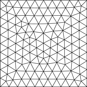
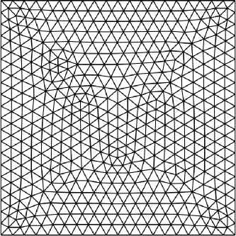
Figure 1. The triangular meshes with mesh size $h=1/10$ (left) and $h=1/20$ for Example 1.

$m$		$\|e_{u}\|_{L^{2}(\Omega)}$	order	$|\!|\!|e_{u}|\!|\!|_{u}$	order	$\|e_{\boldsymbol{\mathrm{p}}}\|_{\boldsymbol{\mathrm{L}}^{2}(\Omega)}$	order	$|\!|\!|e_{\boldsymbol{\mathrm{p}}}|\!|\!|_{\boldsymbol{\mathrm{p}}}$	order
$1$	1	1.0602e-01	-	2.5550e-00	-	1.1553e-00	-	2.9109e+01	-
	2	3.0872e-02	1.80	1.2677e-00	1.01	3.3347e-01	1.80	1.5319e+01	0.93
	3	8.3590e-03	1.90	6.3053e-01	1.01	8.7712e-02	1.90	7.9176e+00	0.95
	4	2.1548e-03	1.96	3.1463e-01	1.00	2.2647e-02	1.96	4.0133e+00	0.98
	5	5.4473e-04	1.98	1.5723e-02	1.00	5.7033e-03	1.98	2.0137e+00	1.00
$2$	1	5.5862e-02	-	9.3425e-01	-	9.1461e-01	-	8.0168e+00	-
	2	1.8898e-02	1.57	2.8628e-01	1.71	2.7402e-01	1.73	1.7807e+00	2.17
	3	4.9746e-03	1.93	7.3469e-02	1.93	7.1190e-02	1.95	4.1888e-01	2.08
	4	1.2538e-03	1.99	1.8776e-02	1.98	1.8016e-02	1.98	1.0111e-01	2.03
	5	3.1393e-04	2.00	4.7137e-03	1.99	4.5126e-03	2.00	2.4633e-02	2.02
$3$	1	5.2485e-03	-	1.6872e-01	-	1.2492e-01	-	3.7196e+00	-
	2	3.9516e-04	3.73	1.9952e-02	3.07	9.2700e-03	3.75	4.6565e-01	2.95
	3	2.1869e-05	4.17	2.0437e-03	3.28	5.9833e-04	3.95	6.0447e-02	2.97
	4	1.1300e-06	4.27	2.2652e-04	3.17	3.8808e-05	3.95	7.7175e-03	2.97
	5	6.0716e-08	4.07	2.7352e-05	3.05	2.4584e-06	3.98	9.7343e-04	2.99

Table 2. Example 1. The errors $e_{u}=u-u_{h},e_{\boldsymbol{\mathrm{p}}}=\boldsymbol{\mathrm{p}}-\boldsymbol{\mathrm{p}}_{h}$, and the orders of convergence with the spaces $\boldsymbol{\mathrm{U}}_{h}^{m}\times\widehat{V}_{h}^{m}(1\leq m\leq 3)$.

$m$		$\|e_{u}\|_{L^{2}(\Omega)}$	order	$|\!|\!|e_{u}|\!|\!|_{u}$	order	$\|e_{\boldsymbol{\mathrm{p}}}\|_{\boldsymbol{\mathrm{L}}^{2}(\Omega)}$	order	$|\!|\!|e_{\boldsymbol{\mathrm{p}}}|\!|\!|_{\boldsymbol{\mathrm{p}}}$	order
$2$	1	6.8296e-02	-	2.4561e-00	-	9.1461e-01	-	8.0168e+00	-
	2	1.7533e-02	1.96	1.2484e-00	0.97	2.7402e-01	1.73	1.7807e+00	2.17
	3	4.4126e-03	1.99	6.2683e-01	0.99	7.1190e-02	1.95	4.1888e-01	2.08
	4	1.1050e-03	2.00	3.3137e-01	1.00	1.8016e-02	1.98	1.0111e-01	2.03
	5	2.7636e-04	2.00	1.5691e-01	1.00	4.5126e-03	2.00	2.4633e-02	2.02
$3$	1	4.9662e-03	-	3.8263e-01	-	1.2492e-01	-	3.7196e+00	-
	2	6.3248e-04	2.97	9.7317e-02	1.97	9.2700e-03	3.75	4.6565e-01	2.95
	3	7.9437e-05	2.99	2.4434e-02	1.99	5.9833e-04	3.95	6.0447e-02	2.97
	4	9.9415e-06	3.00	6.1151e-03	2.00	3.8808e-05	3.95	7.7175e-03	2.97
	5	1.2430e-06	3.00	1.5291e-03	2.00	2.4584e-06	3.98	9.7343e-04	2.99

Table 3. Example 1. The errors $e_{u}=u-u_{h},e_{\boldsymbol{\mathrm{p}}}=\boldsymbol{\mathrm{p}}-\boldsymbol{\mathrm{p}}_{h}$, and the orders of convergence with the spaces $\boldsymbol{\mathrm{U}}_{h}^{m}\times\widehat{V}_{h}^{m-1}(2\leq m\leq 3)$.

Example 2

In this example, we consider the sample problem as in Example 1. But we use a sequence of polygonal meshes consisting of elements with various geometries (see Fig. 2), which are generated by PolyMesher [25]. We only solve the flux, and we present the corresponding errors in the energy norm and $L^{2}$ norm and their respective computed rates in Tab.  4. Again we observe the optimal convergence for both norms when $m$ is odd. For even $m$, $\|\boldsymbol{\mathrm{p}}-\boldsymbol{\mathrm{p}}_{h}\|_{\boldsymbol{\mathrm{L}}^{2}(\Omega)}$ tends to zero in a suboptimal way. To apply the method on meshes with different geometry, it is an advantage inherited from the DG method. On such meshes, the convergence order is agreed with our error estimates again.

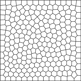
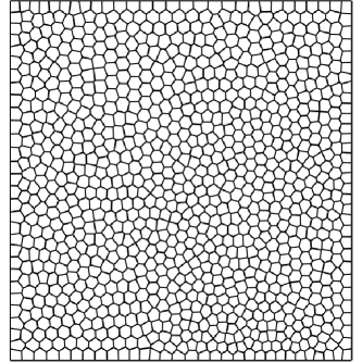
Figure 2. The polygonal meshes with 250 elements (left) / 1000 elements (right).

$m$	DOFs	$\|e_{\boldsymbol{\mathrm{p}}}\|_{\boldsymbol{\mathrm{L}}^{2}(\Omega)}$	order	$\|e_{\boldsymbol{\mathrm{p}}}\|_{\boldsymbol{\mathrm{p}}}$	order
$1$	500	1.0485e-00	-	2.6456e+01	-
	2000	2.7316e-01	1.94	1.3244e+01	0.99
	8000	6.5948e-02	2.05	6.5998e-00	1.00
	32000	1.6203e-02	2.03	3.2658e-00	1.01
$2$	500	4.4773e-01	-	6.1493e-00	-
	2000	1.2630e-01	1.83	1.3713e-00	2.16
	8000	3.0209e-02	2.06	3.3353e-01	2.03
	32000	7.4860e-03	2.01	8.2873e-02	2.01
$3$	500	1.6412e-01	-	4.5508e-00	-
	2000	1.0449e-02	3.97	6.2226e-01	2.88
	8000	6.3315e-04	4.05	8.1210e-02	2.95
	32000	3.8188e-05	4.03	1.0205e-02	2.99

Table 4. Example 2. The errors $e_{\boldsymbol{\mathrm{p}}}=\boldsymbol{\mathrm{p}}-\boldsymbol{\mathrm{p}}_{h}$, and the orders of convergence with the spaces $\boldsymbol{\mathrm{U}}_{h}^{m}(1\leq m\leq 3)$.

Example 3

In this example, we consider the mild wave front problem, which is the Poisson equation on the unit square with Dirichlet boundary conditions. The data functions $f$ and $g$ are selected such that the exact solution is

$$u(x,y)=\arctan(\alpha(r-r_{0})),\quad(x,y)\in[0,1]^{2},$$

where $r=\sqrt{(x-x_{0})^{2}+(y-y_{0})^{2}}$. The mild wave front uses $(x_{0},y_{0})=(-0.05,-0.05)$, $r_{0}=0.7$, $\alpha=10$ and it is a problem of near singularities. For this problem, the high-order accuracy is preferred [23]. We use a sequence of quasi-uniform triangular meshes (see Fig. 3) and we solve the problem with spaces $\boldsymbol{\mathrm{U}}_{h}^{m}\times\widehat{V}_{h}^{m}(1\leq m\leq 3)$. We list the errors in approximation to $\boldsymbol{\mathrm{p}}$ and $u$ in Tab.  5. It is clear that the proposed method yields the same convergence rates as the Example 1, which validates our theoretical estimates.

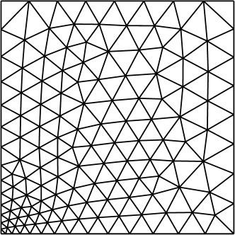
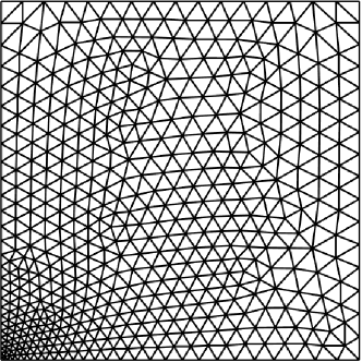
Figure 3. The triangular meshes with 246 elements (left) and 984 elements (right) for Example 3.

$m$		$\|e_{u}\|_{L^{2}(\Omega)}$	order	$|\!|\!|e_{u}|\!|\!|_{u}$	order	$\|e_{\boldsymbol{\mathrm{p}}}\|_{\boldsymbol{\mathrm{L}}^{2}(\Omega)}$	order	$|\!|\!|e_{\boldsymbol{\mathrm{p}}}|\!|\!|_{\boldsymbol{\mathrm{p}}}$	order
$1$	1	4.3807e-02	-	4.9822e-01	-	1.1553e-00	-	1.0256e+01	-
	2	1.6473e-02	1.41	4.0917e-01	1.03	3.3347e-01	1.80	5.3347e+00	0.95
	3	3.5661e-03	2.21	1.9515e-01	1.07	8.7712e-02	1.90	2.6486e+00	1.01
	4	8.6682e-04	2.03	9.5962e-02	1.02	2.2647e-02	1.96	1.3231e+00	1.00
	5	2.1263e-04	2.03	4.7761e-02	1.00	5.7033e-03	1.98	6.6057e-01	1.00
$2$	1	1.5200e-02	-	2.9032e-01	-	2.4411e-01	-	5.6918e+00	-
	2	5.3703e-03	1.51	9.0132e-02	1.68	8.9263e-02	1.45	1.3870e+00	2.03
	3	1.4510e-03	1.89	2.5011e-02	1.85	2.5413e-02	1.82	3.1295e-01	2.10
	4	3.6778e-04	1.98	6.5013e-02	2.00	6.7113e-03	1.92	7.1999e-02	2.11
	5	9.1211e-05	2.01	1.6380e-03	1.98	1.6989e-03	1.99	1.7550e-02	2.03
$3$	1	1.0333e-02	-	8.0091e-02	-	2.0391e-01	-	5.8500e+00	-
	2	1.1023e-03	3.23	1.2076e-02	2.72	1.7701e-02	3.52	9.7265e-01	2.59
	3	6.7612e-05	4.03	1.2368e-03	3.28	1.1398e-03	3.96	1.3999e-01	2.80
	4	4.2528e-06	4.00	1.2956e-04	3.26	7.4761e-05	3.93	1.8073e-02	2.96
	5	2.2322e-07	4.12	1.4319e-05	3.17	4.7259e-06	3.98	2.2425e-03	3.01

Table 5. Example 3. The errors $e_{u}=u-u_{h},e_{\boldsymbol{\mathrm{p}}}=\boldsymbol{\mathrm{p}}-\boldsymbol{\mathrm{p}}_{h}$, and the orders of convergence with the spaces $\boldsymbol{\mathrm{U}}_{h}^{m}\times\widehat{V}_{h}^{m}(1\leq m\leq 3)$.

Example 4

In this example, we exhibit the performance of the proposed method with the problem with a corner singularity. We consider the L-shaped domain $\Omega=[-1,1]^{2}\backslash[0,1)\times(-1,0]$ and we use a series of triangular meshes, see Fig. 4. Following [22], we let the exact solution be

$$u(r,\theta)=r^{5/3}\sin(5\theta/3)$$

in polar coordinate and impose the Dirichlet boundary condition. The data $f$ and the function $g$ are chosen accordingly. We notice that $u(r,\theta)$ only belongs to $H^{2+s}$ with $s<2/3$. In Tab. 6, we list the errors measured in the energy norm and $L^{2}$ norm for both flux and pressure. Here we observe that the error $|\!|\!|\boldsymbol{\mathrm{p}}-\boldsymbol{\mathrm{p}}_{h}|\!|\!|_{\boldsymbol{\mathrm{p}}}$ decreases at the rate $O(h^{2/3})$ which matches with the fact that $\boldsymbol{\mathrm{p}}$ only belongs to $H^{5/3-\varepsilon}(\Omega)$. The computed orders of $\|\boldsymbol{\mathrm{p}}-\boldsymbol{\mathrm{p}}_{h}\|_{L^{2}(\Omega)}$, $|\!|\!|u-u_{h}|\!|\!|_{u}$ and $\|u-u_{h}\|_{L^{2}(\Omega)}$ are about $1$. A possible explanation of the rates may be traced back to the lack of $H^{3}$-regularity of the exact solution on the whole domain.

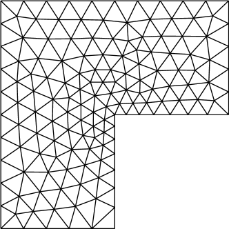
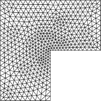
Figure 4. The triangular meshes with 250 elements (left) and 1000 elements for Example 3.

$m$		$\|e_{u}\|_{L^{2}(\Omega)}$	order	$|\!|\!|e_{u}|\!|\!|_{u}$	order	$\|e_{\boldsymbol{\mathrm{p}}}\|_{\boldsymbol{\mathrm{L}}^{2}(\Omega)}$	order	$|\!|\!|e_{\boldsymbol{\mathrm{p}}}|\!|\!|_{\boldsymbol{\mathrm{p}}}$	order
$1$	1	4.5059e-03	-	1.5490e-01	-	3.9382e-02	-	4.2524e-02	-
	2	1.3528e-03	1.73	7.7746e-02	0.99	1.8681e-02	1.07	2.5539e-02	0.73
	3	4.0795e-04	1.73	3.8900e-02	1.00	9.3165e-03	1.00	1.5859e-02	0.68
	4	1.3376e-04	1.61	1.9563e-02	1.00	4.5537e-03	1.03	9.9689e-03	0.67
	5	5.2105e-05	1.36	9.7263e-03	1.00	2.2927e-03	1.00	6.2815e-03	0.67
$2$	1	2.2627e-03	-	9.3186e-03	-	3.4672e-02	-	5.1619e-02	-
	2	6.8183e-04	1.73	2.6548e-03	1.81	1.6061e-02	1.11	2.9373e-02	0.81
	3	2.3956e-04	1.51	9.2329e-04	1.52	8.0869e-03	0.99	1.8481e-02	0.67
	4	1.0011e-04	1.99	3.7505e-04	1.29	4.0509e-03	1.26	1.1383e-02	0.68
	5	4.5381e-05	1.13	1.7137e-04	1.12	2.0293e-03	1.00	7.0855e-03	0.68
$3$	1	2.5557e-03	-	1.1823e-02	-	4.1292e-02	-	5.7175e-02	-
	2	8.6799e-04	1.55	4.1778e-03	1.50	1.9767e-02	1.06	3.0635e-02	0.90
	3	3.3653e-04	1.36	1.4712e-03	1.50	9.6459e-03	1.03	1.0801e-02	0.76
	4	1.5550e-04	1.13	5.9787e-04	1.29	4.9361e-05	0.98	1.1136e-02	0.68
	5	7.5031e-05	1.06	2.8188e-04	1.08	2.5011e-05	0.99	6.9361e-03	0.68

Table 6. Example 4. The errors $e_{u}=u-u_{h},e_{\boldsymbol{\mathrm{p}}}=\boldsymbol{\mathrm{p}}-\boldsymbol{\mathrm{p}}_{h}$, and the orders of convergence with the spaces $\boldsymbol{\mathrm{U}}_{h}^{m}\times\widehat{V}_{h}^{m}(1\leq m\leq 3)$.

Example 5

We consider a three-dimensional Poisson problem on a unit cube $\Omega=[0,1]^{3}$. The domain is partitioned into a series of tetrahedral meshes with mesh size $h=1/5,1/10,1/20,1/40$ by Gmsh [15]. The exact solution is taken as

$$u(x,y,z)=\sin(2\pi x)\sin(2\pi y)\sin(2\pi z),$$

and the Dirichlet function $g$ and the source term $f$ are taken suitably. We use the spaces $\boldsymbol{\mathrm{U}}_{h}^{m}\times\widehat{V}_{h}^{m}(1\leq m\leq 3)$ to approximate $\boldsymbol{\mathrm{p}}$ and $u$, respectively. The numerical results are presented in Tab. 7. We still observe the optimal convergence rate for $\boldsymbol{\mathrm{p}}_{h}$ under $\boldsymbol{\mathrm{L}}^{2}$ norm when $m$ is odd, and all computed convergence orders agree with the theoretical analysis.

$m$		$\|e_{u}\|_{L^{2}(\Omega)}$	order	$|\!|\!|e_{u}|\!|\!|_{u}$	order	$\|e_{\boldsymbol{\mathrm{p}}}\|_{\boldsymbol{\mathrm{L}}^{2}(\Omega)}$	order	$|\!|\!|e_{\boldsymbol{\mathrm{p}}}|\!|\!|_{\boldsymbol{\mathrm{p}}}$	order
$1$	1	2.0159e-01	-	2.6227e-00	-	1.4772e-00	-	2.0737e+01	-
	2	6.7739e-02	1.76	1.4117e-00	0.89	4.3453e-01	1.80	1.0927e+01	0.93
	3	1.8200e-02	1.90	7.3125e-01	0.95	1.1641e-02	1.90	5.4683e+00	0.99
	4	4.6456e-03	1.96	3.6691e-01	1.00	2.9923e-02	1.96	2.7331e+00	1.00
$2$	1	2.8293e-02	-	7.6111e-01	-	3.6002e-01	-	7.0288e+00	-
	2	9.1341e-02	1.63	2.2963e-01	1.73	1.0421e-01	1.79	1.7895e+00	1.97
	3	2.5926e-03	1.82	6.1281e-02	1.91	2.8129e-02	1.89	4.6372e-01	1.95
	4	6.8012e-04	1.93	1.5021e-02	2.01	7.2823e-03	1.95	1.1599e-01	2.00
$3$	1	7.2877e-03	-	1.8326e-01	-	1.7658e-01	-	3.0434e+00	-
	2	7.3997e-04	3.30	2.1873e-02	3.06	1.3510e-02	3.71	3.9250e-01	2.96
	3	5.6061e-05	3.73	2.7168e-03	3.28	9.2336e-04	3.87	5.1203e-02	3.01
	4	3.6203e-06	3.96	3.3962e-04	3.17	5.9170e-05	3.96	6.4123e-03	3.00

Table 7. Example 5. The errors $e_{u}=u-u_{h},e_{\boldsymbol{\mathrm{p}}}=\boldsymbol{\mathrm{p}}-\boldsymbol{\mathrm{p}}_{h}$, and the orders of convergence with the spaces $\boldsymbol{\mathrm{U}}_{h}^{m}\times\widehat{V}_{h}^{m}(1\leq m\leq 3)$.

5.2. Efficiency comparison

The number of the degrees of freedom of a discretized system is a suitable indicator for the efficiency, as illustrated by Hughes et al in [17]. In our method, the accuracy of $\boldsymbol{\mathrm{p}}_{h}$ determines the convergence behavior of the pressure. Thus, to show the efficiency of the proposed method, we make a comparison between the standard least squares discontinuous finite element method presented in Section 2 and the proposed method by comparing the error of the numerical flux $\boldsymbol{\mathrm{p}}_{h}$.

For both methods, we select the finite element spaces of equal order for solving the Poisson problem. Here we solve the problems that are taken from the Example 1 and Example 5 for two and three dimensional case, respectively. We implement the two methods on successively refined meshes. In Fig. 5, we plot the errors of numerical flux in the DLS energy norm $\|\cdot\|_{\boldsymbol{\mathrm{p}}}$ against the number of degrees of freedom with $1\leq m\leq 3$ in two and three dimension. All convergence orders are in perfect agreement with the theoretical results.

There are two points notable for us. To achieve the same accuracy, the proposed method uses much less DOFs than the DLS finite element method. The saving of number of DOFs is more remarkable for higher order approximation. For $d=2$, the number of DOFs used in our method is about $36\%$ of that in DLS method for linear approximation to achieve the same accuracy. Meanwhile, the number of DOFs used in our method is about $31\%$ and $27\%$ of the number of DOFs used in DLS method for $m=2$ and $3$, respectively (see Fig. 5). In Fig. 5, one may see that the saving of number DOFs for 3D problems is even more significant than 2D problems. For $d=3$, the percentages of number of DOFs reduce to about $30\%$, $12\%$, and $5\%$ of that in DLS method for $m=1$, $2$, and $3$, respectively.

Let us note at last that the numerical flux $\boldsymbol{\mathrm{p}}_{h}$ obtained by our method is locally irrotational, which is a natural property as the gradient of a function.

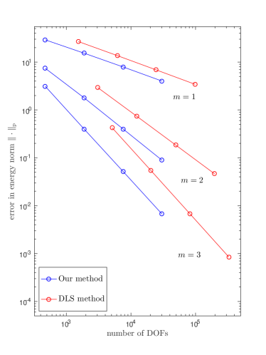
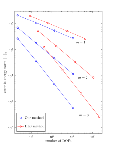
Figure 5. Comparison of the error $\|\boldsymbol{\mathrm{p}}-\boldsymbol{\mathrm{p}}_{h}\|_{\boldsymbol{\mathrm{p}}}$ in number of DOFs by two methods with $m=1,2,3$ in two dimension (left) and three dimension (right).

6. Conclusion

We proposed a sequential least squares finite element method for the Poisson equation. The novel piecewisely irrotational approximation space is constructed by solving local least squares problem and we use this space to decouple the least squares minimization problem. We proved the convergences for pressure and flux in $L^{2}$ norm and energy norm. By a series of numerical results, not only the error estimates are verified, but also we exhibited the flexibility and the great efficiency of our method.

Appendix A

In Appendix, we present some details of the reconstruction process. We first give an example of constructing the element patch in two dimensional case. For element $K$, the construction of $S(K)$ with $\#S(K)=15$ is presented in Fig. 6.

(a) $S_{0}(K)=\{K\}$

(b) $S_{1}(K)$

(c) $S(K)$

(d) $S_{2}(K)$

Figure 6. Build patch for element $K$ with $\#S(K)=15$

Then we give more details about the space $\boldsymbol{\mathrm{U}}_{h}^{m}$. As we mentioned before, the operator $\mathcal{R}^{m}$ embeds the space $\boldsymbol{\mathrm{C}}^{0}(\Omega)\cap H(\mathrm{curl}^{0};\Omega)$ to the piecewise irrotational polynomial space of degree $m$ by solving the local least squares problem. We define $\boldsymbol{\mathrm{w}}_{K}^{i}(\boldsymbol{x})\in\boldsymbol{\mathrm{C}}^{0}(\Omega)(1\leq i\leq d)$ that

$$\boldsymbol{\mathrm{w}}_{K}^{i}(\boldsymbol{x})=\begin{cases}\boldsymbol{e}_{i},\quad\boldsymbol{x}=\boldsymbol{x}_{K},\\ \boldsymbol{0},\quad\boldsymbol{x}\in\widetilde{K},\quad\widetilde{K}\neq K,\end{cases}\quad\forall K\in\mathcal{T}_{h},$$

where $\boldsymbol{e}_{i}$ is a $d\times 1$ unit vector whose $i$-th entry is $1$. Then $\boldsymbol{\mathrm{U}}_{h}^{m}=\text{span}\{\boldsymbol{\mathrm{\lambda}}_{K}^{i}\ |\ \boldsymbol{\mathrm{\lambda}}_{K}^{i}=\mathcal{R}^{m}\boldsymbol{\mathrm{w}}_{K}^{i},\ 1\leq i\leq d,\ K\in\mathcal{T}_{h}\}$, and one can write the operator $\mathcal{R}^{m}$ in an explicit way: for a function $\boldsymbol{\mathrm{g}}=(g^{1},\cdots,g^{d})\in\boldsymbol{\mathrm{C}}^{0}(\Omega)\cap H(\mathrm{curl}^{0};\Omega)$ we have

$$\mathcal{R}^{m}\boldsymbol{\mathrm{g}}=\sum_{K\in\mathcal{T}_{h}}\sum_{i=1}^{d}g^{i}(\boldsymbol{x}_{K})\boldsymbol{\mathrm{\lambda}}_{K}^{i}(\boldsymbol{x}).$$

Clearly, the number of DOFs of our method is always $d$ times the number of elements in partition.

Further, we give some details about the computer implementation of the reconstructed space. We take the case $d=2$ to illustrate. We first outline the bases of the space $\boldsymbol{\mathrm{S}}_{m}(D)$, it is easily verified that for $d=2$,

$$\boldsymbol{\mathrm{S}}_{1}(D)=\left\{\begin{pmatrix}1\\ 0\\ \end{pmatrix},\begin{pmatrix}0\\ 1\\ \end{pmatrix},\begin{pmatrix}x\\ 0\\ \end{pmatrix},\begin{pmatrix}0\\ y\\ \end{pmatrix},\begin{pmatrix}y\\ x\\ \end{pmatrix}\right\}.$$

Similarly for $m=2,3$, there is

$$\boldsymbol{\mathrm{S}}_{2}(D)=\boldsymbol{\mathrm{S}}_{1}(D)\cup \left\{\begin{pmatrix}x^{2}\\ 0\\ \end{pmatrix},\begin{pmatrix}2xy\\ x^{2}\\ \end{pmatrix},\begin{pmatrix}y^{2}\\ 2xy\\ \end{pmatrix},\begin{pmatrix}0\\ y^{2}\\ \end{pmatrix}\right\},$$

$$\boldsymbol{\mathrm{S}}_{3}(D)=\boldsymbol{\mathrm{S}}_{2}(D)\cup \left\{\begin{pmatrix}x^{3}\\ 0\\ \end{pmatrix},\begin{pmatrix}3x^{2}\\ y\\ \end{pmatrix},\begin{pmatrix}2xy^{2}\\ 2x^{2}y\\ \end{pmatrix},\begin{pmatrix}y^{3}\\ 3xy^{2}\\ \end{pmatrix},\begin{pmatrix}0\\ y^{3}\\ \end{pmatrix}\right\}.$$

Then we shall solve the least squares problem (11) on every element. We take $K_{0}$ and $m=1$ for an instance (see Fig. 7), and we let $S(K_{0})=\left\{K_{0},K_{1},K_{2},K_{3}\right\}$ where $K_{i}(i=1,2,3)$ are the adjacent edge-neighbouring elements of $K_{0}$. We denote by $\boldsymbol{x}_{i}=(x_{i},y_{i})$ the barycenter of the element $K_{i}$ and we obtain the collocation points set $\mathcal{I}_{K_{0}}=\left\{\boldsymbol{x}_{0},\boldsymbol{x}_{1},\boldsymbol{x}_{2},\boldsymbol{x}_{3}\right\}$.

Figure 7. $K$ and its neighbours

Then for the function $\boldsymbol{\mathrm{g}}=(g^{1},g^{2})\in\boldsymbol{\mathrm{C}}^{0}(\Omega)\cap H(\mathrm{curl}^{0};\Omega)$ the least squares problem on $K_{0}$ reads

$$\mathop{\arg\min}_{\boldsymbol{a}\in\mathbb{R}^{5}}\sum_{i=0}^{3}\left\|a_{0}\begin{pmatrix}1\\ 0\\ \end{pmatrix}+a_{1}\begin{pmatrix}0\\ 1\\ \end{pmatrix}+a_{2}\begin{pmatrix}x_{i}\\ 0\\ \end{pmatrix}+a_{3}\begin{pmatrix}0\\ y_{i}\\ \end{pmatrix}+a_{4}\begin{pmatrix}y_{i}\\ x_{i}\\ \end{pmatrix}-\begin{pmatrix}g^{1}(x_{i})\\ g^{2}(y_{i})\\ \end{pmatrix}\right\|^{2}.$$

It is easy to obtain its unique solution

$$\boldsymbol{a}=(A^{T}A)^{-1}A^{T}\boldsymbol{q},$$

where

$$A=\begin{bmatrix}1&0&x_{0}&0&y_{0}\\ 0&1&0&y_{0}&x_{0}\\ 1&0&x_{1}&0&y_{1}\\ 0&1&0&y_{1}&x_{1}\\ 1&0&x_{2}&0&y_{2}\\ 0&1&0&y_{2}&x_{2}\\ 1&0&x_{3}&0&y_{3}\\ 0&1&0&y_{3}&x_{3}\\ \end{bmatrix},\qquad\boldsymbol{q}=\begin{bmatrix}g^{1}(x_{0})\\ g^{2}(y_{0})\\ g^{1}(x_{1})\\ g^{2}(y_{1})\\ g^{1}(x_{2})\\ g^{2}(y_{2})\\ g^{1}(x_{3})\\ g^{2}(y_{3})\\ \end{bmatrix}.$$

We notice that the matrix $(A^{T}A)^{-1}A^{T}$ is independent of the function $\boldsymbol{\mathrm{g}}$ and includes all information of the function $\boldsymbol{\mathrm{\lambda}}_{K_{j}}^{i}(j=0,1,2,3,\ i=1,2)$ on the element $K_{0}$. Thus we could store the matrix $(A^{T}A)^{-1}A^{T}$ for every element to represent our approximation space. The idea of the implementation could be adapted to the high-order accuracy case and the high dimensional problem without any difficulty.

References

- [1] P. F. Antonietti, L. Beirão da Veiga, and M. Verani, A mimetic discretization of elliptic obstacle problems, Math. Comp. 82 (2013), no. 283, 1379–1400.
- [2] D. N. Arnold, An interior penalty finite element method with discontinuous elements, SIAM J. Numer. Anal. 19 (1982), no. 4, 742–760.
- [3] D. N. Arnold, F. Brezzi, B. Cockburn, and L. D. Marini, Unified analysis of discontinuous Galerkin methods for elliptic problems, SIAM J. Numer. Anal. 39 (2001/02), no. 5, 1749–1779.
- [4] A. K. Aziz, R. B. Kellogg, and A. B. Stephens, Least squares methods for elliptic systems, Math. Comp. 44 (1985), no. 169, 53–70. MR 771030
- [5] Rickard Bensow and Mats G. Larson, Discontinuous least-squares finite element method for the div-curl problem, Numer. Math. 101 (2005), no. 4, 601–617. MR 2195400
- [6] Rickard E. Bensow and Mats G. Larson, Discontinuous/continuous least-squares finite element methods for elliptic problems, Math. Models Methods Appl. Sci. 15 (2005), no. 6, 825–842.
- [7] Pavel Bochev, James Lai, and Luke Olson, A locally conservative, discontinuous least-squares finite element method for the Stokes equations, Internat. J. Numer. Methods Fluids 68 (2012), no. 6, 782–804. MR 2878612
- [8] by same author, A non-conforming least-squares finite element method for incompressible fluid flow problems, Internat. J. Numer. Methods Fluids 72 (2013), no. 3, 375–402. MR 3049438
- [9] Pavel B. Bochev and Max D. Gunzburger, Accuracy of least-squares methods for the Navier-Stokes equations, Comput. & Fluids 22 (1993), no. 4-5, 549–563.
- [10] by same author, Finite element methods of least-squares type, SIAM Rev. 40 (1998), no. 4, 789–837. MR 1659689
- [11] by same author, Least-squares finite element methods, Applied Mathematical Sciences, vol. 166, Springer, New York, 2009.
- [12] James H. Bramble, Raytcho D. Lazarov, and Joseph E. Pasciak, A least-squares approach based on a discrete minus one inner product for first order systems, Math. Comp. 66 (1997), no. 219, 935–955. MR 1415797
- [13] Ching Lung Chang, An error estimate of the least squares finite element method for the Stokes problem in three dimensions, Math. Comp. 63 (1994), no. 207, 41–50. MR 1234425
- [14] P. G. Ciarlet, The Finite Element Method for Elliptic Problems, Classics in Applied Mathematics, vol. 40, Society for Industrial and Applied Mathematics (SIAM), Philadelphia, PA, 2002, Reprint of the 1978 original [North-Holland, Amsterdam; MR0520174 (58 #25001)].
- [15] C. Geuzaine and J. F. Remacle, Gmsh: A 3-D finite element mesh generator with built-in pre- and post-processing facilities, Internat. J. Numer. Methods Engrg. 79 (2009), no. 11, 1309–1331.
- [16] Vivette Girault and Pierre Arnaud Raviart, Finite element methods for navier-stokes equations: Theory and algorithms, Springer-Verlag, 1986.
- [17] Thomas J. R. Hughes, Gerald Engel, Luca Mazzei, and Mats G. Larson, A comparison of discontinuous and continuous Galerkin methods based on error estimates, conservation, robustness and efficiency, Discontinuous Galerkin methods (Newport, RI, 1999), Lect. Notes Comput. Sci. Eng., vol. 11, Springer, Berlin, 2000, pp. 135–146. MR 1842169
- [18] Bo-Nan Jiang and Louis A. Povinelli, Optimal least-squares finite element method for elliptic problems, Comput. Methods Appl. Mech. Engrg. 102 (1993), no. 2, 199–212.
- [19] R. Li, P. B. Ming, Z. Y. Sun, F. Y. Yang, and Z. J. Yang, A discontinuous Galerkin method by patch reconstruction for biharmonic problem, accepted by Journal of Computational Mathematics, arXiv:1712.10103 (2017).
- [20] R. Li, P. B. Ming, Z. Y. Sun, and Z. J. Yang, An arbitrary-order discontinuous Galerkin method with one unknown per element, arXiv:1803.00378 (2018).
- [21] R. Li, P. B. Ming, and F. Tang, An efficient high order heterogeneous multiscale method for elliptic problems, Multiscale Model. Simul. 10 (2012), no. 1, 259–283.
- [22] William F. Mitchell, A collection of 2D elliptic problems for testing adaptive grid refinement algorithms, Appl. Math. Comput. 220 (2013), 350–364.
- [23] William F. Mitchell, How high a degree is high enough for high order finite elements?, Procedia Computer Science 51 (2015), 246 – 255, International Conference On Computational Science, ICCS 2015.
- [24] A. I. Pehlivanov, G. F. Carey, and R. D. Lazarov, Least-squares mixed finite elements for second-order elliptic problems, SIAM J. Numer. Anal. 31 (1994), no. 5, 1368–1377. MR 1293520
- [25] C. Talischi, G. H. Paulino, A. Pereira, and I. F. M. Menezes, PolyMesher: a general-purpose mesh generator for polygonal elements written in Matlab, Struct. Multidiscip. Optim. 45 (2012), no. 3, 309–328.
- [26] Xiu Ye and Shangyou Zhang, A discontinuous least-squares finite-element method for second-order elliptic equations, International Journal of Computer Mathematics 96 (2019), no. 3, 557–567.
- [27] O. C. Zienkiewicz, R. L. Taylor, S. J. Sherwin, and J. Peiró, On discontinuous Galerkin methods, Internat. J. Numer. Methods Engrg. 58 (2003), no. 8, 1119–1148.