Collisions of acoustic solitons and their electric fields in plasmas at critical compositions

Abstract

Acoustic solitons obtained through a reductive perturbation scheme are normally governed by a Korteweg-de Vries (KdV) equation. In multispecies plasmas at critical compositions the coefficient of the quadratic nonlinearity vanishes. Extending the analytic treatment then leads to a modified KdV (mKdV) equation, which is characterized by a cubic nonlinearity and is even in the electrostatic potential. The mKdV equation admits solitons having opposite electrostatic polarities, in contrast to KdV solitons which can only be of one polarity at a time. A Hirota formalism has been used to derive the two-soliton solution. That solution covers not only the interaction of same-polarity solitons but also the collision of compressive and rarefactive solitons. For the visualisation of the solutions, the focus is on the details of the interaction region. A novel and detailed discussion is included of typical electric field signatures that are often observed in ionospheric and magnetospheric plasmas. It is argued that these signatures can be attributed to solitons and their interactions. As such, they have received little attention.

1 Introduction

Acoustic solitons in plasmas, obtained through a reductive perturbation theory (RPT), are normally governed by a Korteweg-de Vries equation. The equation was originally derived to model solitary waves observed on the surface of shallow water [Korteweg & de Vries (1895); Ablowitz & Clarkson (1991)], but was seventy years later found to have applications in various other fields of physics, notably in plasmas [Gardner et al. (1967, 1974)]. Because of the algorithmic nature of RPT it became a popular tool in theoretical studies of nonlinear acoustic waves in plasmas, for a variety of different model compositions, resulting in a large number of scholarly publications.

It was also established that equations such as the KdV equation are completely integrable, in the sense that besides the single soliton solution there are also $N$-soliton solutions (for any positive integer $N$) which collide elastically. Even the one-soliton solution shows that there is an intricate relation between the amplitude, width and velocity of the wave. In particular, larger solitons are narrower but travel faster. For a typical two-soliton interaction this means that a later-launched larger soliton will overtake a slower one. After an intricate collision, both emerge unscathed except for small phase shifts. Hence the name “soliton” was coined Zabusky & Kruskal (1965) for the resemblance with interacting particles.

The colloquial term “later-launched” has to be understood as follows. A two-soliton solution is not merely a superposition of two single solitons, as this would be meaningless for a nonlinear equation. Rather, a two-soliton solution has a complicated nonlinear structure which asymptotically reduces to two separated single solitons. During the collision the nonlinearity affects their individual profiles in quite unexpected ways. However, after the collision the two solitons again separate, and resume their initial shapes as if nothing has happened, except for small phase shifts. Indeed, the faster soliton is shifted forward while the slower soliton is shifted backward, relative to the positions where individual solitons would have been had they not collided.

When the plasma model allows for changes in polarities for critical values of the compositional parameters [Das (1975); Das & Tagare (1975); Tagare (1986); Lee (2009); Saini & Shalini (2013)], the analytic treatment then leads to a modified Korteweg-de Vries (mKdV) equation with cubic nonlinearity. The equation is even in the electrostatic potential $\varphi$, thus admitting solitons of opposite electrostatic polarities. In contrast, KdV solitons can only be of one polarity at a time. Recall that the historic application of KdV theory to surface waves on shallow water yielded only compressive solitons, in the shape of humps. Water surfaces do not sustain rarefactive solitons, also called holes or dips.

To study the overtaking interactions between two solitons, Hirota’s bilinear method has been applied, which can deal with any number of interacting waves because the KdV and mKdV equations are completely integrable. Our visualization of two soliton interactions will be focussed on what happens at the center of the interaction region, not only for the electrostatic solitons but also for their derivatives, which yield the electric field profiles. To the best of our knowledge, electric field profiles have not been studied before.

As an aside, there is no Hirota or equivalent formalism that leads to solutions describing head-on collisions, neither for KdV nor mKdV equations. What is available in the literature relies on an extension of the Poincaré-Lighthill-Kuo (PLK) formalism of strained coordinates, which leads to approximate results of limited use [Verheest et al. (2012a, b)]. The shortcoming of the PLK method is that it uses an addition of the amplitudes in an essentially nonlinear problem. Furthermore, its results contradict recent laboratory experiments [Harvey et al. (2010)] and numerical simulations [Kakad et al. (2017); Kumar et al. (2017)].

In Section 2 we recall the essentials of RPT leading to mKdV equations, together with their one-soliton solutions, well studied in the plasma and mathematical physics literature. We summarize the steps of the Hirota bilinear method for the mKdV equation in Section 3. The visualization of these interactions is covered in Section 4, first for a collision of two humps, next for a hump and a hole. Novel features of these interactions, in particular for electric fields, are discussed in Section 5. Electric fields are often seen in ionospheric and magnetospheric satellite observations, but their overtaking interactions have not been studied before. The paper concludes with a brief summary of the results in Section 6.

2 Reductive perturbation formalism and evolution equations

There is a plethora of plasma compositions treated in the literature, allowing critical densities leading to the mKdV equation. These plasmas are usually described by a number of cold and/or warm fluid species, of quite different characteristics, in the presence of some inertialess Boltzmann or nonthermal distributions for the hot species.

RPT rests on two pillars: a suitable stretching of space and time and the expansion of the dependent variables. For the family of KdV-type equations the stretching can be chosen as

$$\xi=\varepsilon(X-VT),\qquad\qquad\tau=\varepsilon^{3}T,$$ (1)

or equivalent choices, with $V$ the linear acoustic phase velocity, $\varepsilon$ a small parameter and $X$ and $T$ the physical space and time coordinates, respectively. This is inspired by the dispersion law for linear waves with frequency $\omega$ and wave number $k$, by taking the limit $k\to 0$ but keeping the phase velocity $\omega/k$ finite, based on the idea that acoustic modes have $\omega$ proportional $k$ to lowest order. For the expansion of the electrostatic potential, $\varphi,$ we take

$$\varphi=\varepsilon\varphi_{1}+\varepsilon^{2}\varphi_{2}+\varepsilon^{3}\varphi_{3}+\ldots,$$ (2)

with similar expansions for the plasma variables like densities, pressures and fluid velocities of the different species.

Applying (1) and (2) to the basic fluid equations and Poisson’s equation produces order by order in $\varepsilon$ sets of equations for the successive $\varphi_{i}$. In the generic case, $\varphi_{1}\equiv 0$ leads to the KdV equation,

$$A\frac{\partial{\varphi_{2}}}{\partial{\tau}}+B\varphi_{2}\,\frac{\partial{\varphi_{2}}}{\partial{\xi}}+\frac{1}{2}\,\frac{\partial{{}^{3}\varphi_{2}}}{\partial{\xi^{3}}}=0.$$ (3)

The coefficients $A$ and $B$ include the compositional plasma parameters and $V$; the latter as a solution of the linear dispersion law is a function of those same parameters. No matter how complicated the plasma model is, one gets the KdV equation (3) which has soliton solutions and other special properties, provided the plasma species obey barotropic pressure-density relations [Verheest (2000)]. Given its ubiquity in physics, this is the best known and most studied nonlinear soliton.

We assume that the plasma composition is critical ($B=0$). Continuing with $\varphi_{1}\not=0$ then leads to the mKdV equation,

$$A\frac{\partial{\varphi_{1}}}{\partial{\tau}}+C\varphi_{1}^{2}\,\frac{\partial{\varphi_{1}}}{\partial{\xi}}+\frac{1}{2}\,\frac{\partial{{}^{3}\varphi_{1}}}{\partial{\xi^{3}}}=0,$$ (4)

where $A$ and $C$ again depend on the plasma parameters and $V$. Perusing the literature, it becomes clear that almost all plasmas need to have at least three constituents before $B=0$ can be imposed under the condition that $V$ annuls the linear dispersion relation.

The earliest examples are plasmas with two cold ion species (one positive, one negative) in the presence of Boltzmann electrons [Das (1975); Das & Tagare (1975); Watanabe (1984); Tagare (1986)]. Later, this was extended to include more cold or warm ion species [Verheest (1988)], and the picture remains unchanged when various nonthermal distributions are introduced for the hot electrons [Verheest (2015)], such as the kappa distribution [Vasyliunas (1968); Summers & Thorne (1991)] and Tsallis nonextensive distribution [Tsallis (1988); Lima et al. (2000)]. The only exception to this three or more species rule is the Cairns distribution [Cairns et al. (1995)] because it admits a critical density in the presence of only one cold ion species. Regardless of the finetuning of the parameters needed for criticality, mKdV solitons were even observed experimentally in multi-ion plasmas and their collision properties were investigated by numerically solving the mKdV equation [Nakamura & Tsukabayashi (2009)].

Note that the mKdV equation (4) is invariant under the change $\varphi$ to $-\varphi$. As a consequence of this uncommon property, every positive polarity soliton has an equivalent negative one. The one-soliton solution of (4) is well known,

$$\varphi_{1}=\pm\sqrt{\frac{6U\!A}{C}}\,{\rm sech}\left[\sqrt{2U\!A}(\xi-U\tau)\right],$$ (5)

where $U$ is an arbitrary velocity, in the frame moving with velocity $V$ with respect to an inertial observer. On the other hand, the two-soliton solution is much less known in the context of plasma physics, and will therefore be the main focus of our efforts in the present paper.

In what follows, we will start from a generic form with coefficients chosen such that the application of Hirota’s formalism [Hirota (1971, 1972, 2004)] is as simple as possible [Drazin & Johnson (1989)]. A change of variables,

$$\xi=2x\,\sqrt{\frac{3}{C}},\qquad\tau=48t\,\frac{A}{C}\,\sqrt{\frac{3}{C}},\qquad\varphi_{1}=u,$$ (6)

transforms the mKdV equation (4) into

$$u_{t}+24u^{2}u_{x}+u_{xxx}=0.$$ (7)

This transformation requires that $C>0$ (and $B=0$). The coefficient 24 in (7) is chosen to minimize the numerical factors when applying Hirota’s method, and derivatives are denoted by lower-case subscripts $x$ and $t$, where, for example, $u_{xxx}$ denotes the third derivative of $u$ with respect to $x$. Note that we have transformed the space and time variables, but $u$ remains a normalized electrostatic potential at the lowest nonzero order.

3 Hirota’s bilinear method and soliton solutions

Hirota (1971) developed an ingenious method to find exact $N$-soliton solutions for the KdV equation. The method uses bilinear operators, hence the name Hirota’s bilinear method. It was later shown that the method can be applied to large classes of nonlinear evolution equations, including the mKdV equation.

The key idea is to change the dependent variable so that the given nonlinear equation becomes bilinear in one or more new dependent variables. Once the appropriate bilinear forms have been found, a formal series expansion is used to generate its solutions in an iterative way. If pure solitons exist the iterative process terminates at a certain level and the finite series leads to an exact solution.

Hirota’s method proceeds in three steps: (i) a judicious guess for the transformation of the dependent variable, (ii) writing the transformed equation as a single bilinear equation or a coupled system of bilinear equations, and (iii) using a formal expansion scheme to solve these bilinear equation(s).

Inspiration for the initial step has sometimes come from performing the Painlevé integrability test [Ablowitz & Clarkson (1991); Drazin & Johnson (1989)] of an evolution equation or knowing its $N$-soliton solution from application of the inverse scattering method.

Let us now recall some of the steps for the mKdV equation. Hirota (1971) introduced bilinear differential operators, $D_{x}$ and $D_{t}$, defined for ordered pairs of arbitrary functions $f(x,t)$ and $g(x,t)$, as follows,

$$D_{x}^{m}D_{t}^{n}\{f\mathbf{\cdot}g\}=\left(\frac{\partial{}}{\partial{x}}-\frac{\partial{}}{\partial{x^{\prime}}}\right)^{m}\left(\frac{\partial{}}{\partial{t}}-\frac{\partial{}}{\partial{t^{\prime}}}\right)^{n}f(x,t)g(x^{\prime},t^{\prime})\bigg{|}_{x^{\prime}=x,t^{\prime}=t}\,,$$ (8)

where $m$ and $n$ are nonnegative integers.

Operators like $D_{x}$ and $D_{t}$ are bilinear because of their evident linearity in both arguments $f$ and $g$.

Whereas the KdV equation can be replaced by one bilinear equation [Hirota (1971); Drazin & Johnson (1989)], the mKdV equation (7) requires a coupled system of bilinear equations [Hirota (1972)] because the change of the dependent variable

$$u=\frac{\partial}{\partial x}\Big{(}\arctan\left(\frac{f}{g}\right)\Big{)}=\frac{f_{x}g-fg_{x}}{f^{2}+g^{2}}$$ (9)

involves two functions $f(x,t)$ and $g(x,t)$. Substitution of (9) into (7) yields, after one integration with respect to $x$,

$$(f^{2}+g^{2})(f_{t}g-fg_{t}+f_{xxx}g-3f_{xx}g_{x}+3f_{x}g_{xx}-fg_{xxx})$$

$$-6(fg_{x}-f_{x}g)(f\!\,f_{xx}-f_{x}^{2}+g\!\,g_{xx}-g_{x}^{2})=0.$$ (10)

Setting each term equal to zero results in the following pair of bilinear equations,

$$(D_{t}+D_{x}^{3})\{f\mathbf{\cdot}g\}=0,$$ (11)

$$D_{x}^{2}\{f\mathbf{\cdot}f+g\mathbf{\cdot}g\}=0.$$ (12)

The expansions are

$$f = f_{0}+\varepsilon f_{1}+\varepsilon^{2}f_{2}+\ldots,$$

$$g = g_{0}+\varepsilon g_{1}+\varepsilon^{2}g_{2}+\ldots,$$ (13)

where $f_{0}$ and $g_{0}$ are constants (not both zero to avoid a trivial solution) and $\varepsilon$ is a bookkeeping parameter to disentangle the different orders. Once the successive $f_{i}$ and $g_{i}$ have been computed, one sets $\varepsilon=1$. Doing the computations, one finds from the lowest nonzero order of (12) that either $f_{0}=g_{1}=0$ or $g_{0}=f_{1}=0$. Both choices are equivalent for they amount to a sign change in the polarity of the nonlinear wave.

To derive the one and two-soliton solutions, we continue with $f_{0}=g_{1}=0$. Then, without loss of generality, we normalize $g_{0}=1$ and recover from $f_{1}={\rm e}^{\theta_{1}}$ (in the one-soliton case) the well-known sech solution (5). Here and below one uses the notation $\theta_{i}=k_{i}x-k_{i}^{3}t+\delta_{i}$, which incorporates the linear dispersion $\omega_{i}=k_{i}^{3}$ characterizing the KdV-family. In the two-soliton case, $f_{1}={\rm e}^{\theta_{1}}+{\rm e}^{\theta_{2}}$ and one can set $f_{2}=0$. For one and two-soliton interactions one can shift the origins of $x$ and $t$ so as to absorb $\delta_{i}$, which will henceforth be omitted. The same argument does no longer work for three-soliton interactions (and higher). Suppressing the $\delta_{i}$ then requires non-unit amplitudes $a_{i}={\rm e}^{\delta_{i}}.$

After computing $g_{2}$ and verifying that $g_{i}=0$ for $i\geqslant 3$ and $f_{i}=0$ for $i\geqslant 2$, one obtains

$$f = {\rm e}^{\theta_{1}}+{\rm e}^{\theta_{2}},$$

$$g = 1-\frac{(k_{1}-k_{2})^{2}}{(k_{1}+k_{2})^{2}}\,{\rm e}^{\theta_{1}+\theta_{2}},$$ (14)

and, from (9),

$$u=\frac{k_{1}{\rm e}^{\theta_{1}}+k_{2}{\rm e}^{\theta_{2}}+\displaystyle{\frac{(k_{1}-k_{2})^{2}}{(k_{1}+k_{2})^{2}}}(k_{1}{\rm e}^{\theta_{2}}+k_{2}{\rm e}^{\theta_{1}}){\rm e}^{\theta_{1}+\theta_{2}}}{1+{\rm e}^{2\theta_{1}}+{\rm e}^{2\theta_{2}}+\displaystyle{\frac{8k_{1}k_{2}}{(k_{1}+k_{2})^{2}}}\,{\rm e}^{\theta_{1}+\theta_{2}}+\displaystyle{\frac{(k_{1}-k_{2})^{4}}{(k_{1}+k_{2})^{4}}}\,{\rm e}^{2\theta_{1}+2\theta_{2}}}.$$ (15)

This is a family of two-soliton solutions of (9) with arbitrary constants $k_{1}$ and $k_{2}$. Written as such, it is not readily imagined what the solution looks like. To get an idea of the shape one has to resort to visualizations which will be the focus of the next section. We have also checked that (15) solves the mKdV equation (7), as other (equivalent) expressions of the solution are possible [Anco et al. (2011)].

4 Interaction dynamics of two solitons for the mKdV equation

In this section we will visualize the dynamics of the two-soliton solution (15). The wave numbers $k_{1}$ and $k_{2}$ determine the amplitude and polarity of the two solitons comprised inside (15), and through the linear dispersion, also the phase speed $k_{i}^{2}$. Far away from the collision region, the two solitons each assume the shape of a single soliton (5). The larger the wave number $k_{i}$, the taller the soliton will be and the faster it will travel since the phase velocity equals $k_{i}^{2}$. A positive wave number produces a hump (or bump); a negative wave number produces a hole (sometimes referred to as dip or depression), but both travel to the right.

To visualize the asymptotic behaviour (in particular, separation into individual solitons) we use long time intervals in Figures 1 and 3, typically for $t$ varying between $-40$ and $40$, with large (equal) time steps, e.g., $\Delta t=40$. To zoom into the collision regions, shown in Figures 2 and 4, we let $t$ vary between, say, $-5$ and $5$, and use small (equal) time steps of length 5. All pictures show snapshots of both solitons at various moments in time to locate them on the $x$-axis before, during, and after their collision, going from left to right. The large soliton peaks are easily identified, far away from the interaction region.

4.1 Overtaking of same polarity solitons

Figure 1 illustrate the dynamics of solitons with the same polarity (two humps).

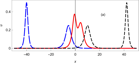
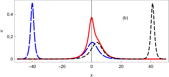
Figure 1: Typical overtaking of a smaller by a larger hump, for (a) $k_{1}=0.5$ and $k_{2}=1$ and (b) $k_{1}=0.3$ and $k_{2}=1$. The curves correspond to $t=-40$ (blue dashed), 0 (red) and 40 (black dotted), where the peaks move to the right as time increases.

The parameters determining the respective shape of the solitons are (a) $k_{1}=0.5$ or (b) $k_{1}=0.3$, and $k_{2}=1$. The curves are shown for $t=-40$ (blue dashed), 0 (red) and 40 (black dotted), where the peaks move to the right as time increases. The pictures for two holes would be the same apart from a vertical flip over the $x$-axis. The distinguishing feature between parts (a) and (b) of Figure 1 is what happens in the interaction zone, details of which are shown in the corresponding graphs in Figure 2.

Although we have graphed the solitons at equal time intervals, it can be seen that when the larger hump has overtaken the smaller one, the net effect is a slight forward shift of the larger soliton. Such shifts do not persist in time, and are only to be compared to what the trajectory of the larger hump would have been, had it been a true one-soliton solution, alone in the physical system. After a while the solitons separate and resume their original shapes. Asymptotically, e.g., for times $t<-40$ or $t>40$, the profile of each soliton becomes undistinguishable from the one-soliton shape.

To start, Figure 1 illustrates how a faster, larger but narrower hump with positive polarity overtakes a slower, smaller but wider one, also with positive polarity, but for different ratios $k_{1}/k_{2}$. By reducing the time step near the overtaking region we show in Figure 2 how the interaction evolves between the larger and the smaller soliton, for the cases shown in Figure 1.

  

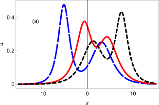
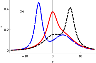
Figure 2: Details of the overtaking interaction of a smaller by a larger hump, for the parameters used in Figure 1. The curves correspond to $t=-5$ (blue dashed), 0 (red) and 5 (black dotted).

The parameters match those in Figure 1, but with smaller time steps, $t=-5$ (blue dashed), 0 (red) and 5 (black dotted).

There are two distinct possibilities. For the first possibility the parameters are chosen such that during the interaction there are at all times two distinct peaks, as shown in Figure 2(a). Thus, as the first peak increases in amplitude and the second peak decreases, it looks as if the larger and the smaller peaks have swapped places. In other words, after the collision the larger soliton is ahead, having undergone a forward phase shift, and mutatis mutandis for the smaller soliton.

The other possibility is that, as we decrease $k_{1}$, keeping $k_{2}$ fixed, the figure changes qualitatively and the two solitons temporarily merge into a single but distorted peak, illustrated in Figure 2(b). This occurs for $k_{1}/k_{2}<0.39$. Indeed, only the ratio is important, as we can, without loss of generality, take $k_{2}=1$ for the largest of the peaks, and $k_{1}<1$ for the smaller one. Analogous results have been found in the mathematics literature [Anco et al. (2011)].

Switching the polarities from positive to negative produces the same type of figures, except that the Figures 1 and 2 are vertically flipped (not shown). All this is reminiscent of what happens for the interaction of KdV solitons, which are always of the same polarity, depending on the sign of $B$ (not shown here, but presented in many papers in the literature).

4.2 Overtaking of opposite polarity solitons

The case of two solitons having opposite polarities leads to graphs which have not been systematically studied before in a plasma physics context. Figure 3 illustrates the dynamics of solitons of the opposite polarity (hump and hole). Figure 4 gives a clearer (zoomed) view of what happens in the interaction zones.

We first illustrate in Figure 3(a) how a faster, larger but narrower hump of positive polarity overtakes a slower, smaller but wider hole of negative polarity. Larger and smaller refer to the absolute values of the amplitudes of the respective solitons.

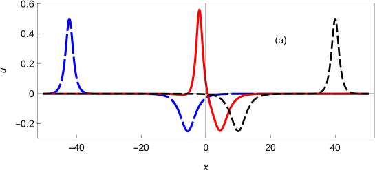
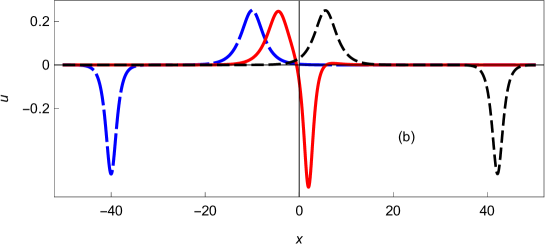
Figure 3: Part (a) shows the typical overtaking of a smaller hole by a larger hump, for $k_{1}=-0.5$ and $k_{2}=1$, whereas part (b) concerns the opposite, where a larger hole overtakes a smaller hump, for $k_{1}=0.5$ and $k_{2}=-1$. The curve coding is as in Figure 1.

Figure 3(b) shows a larger hole overtaking a smaller hump. The parameters are $k_{1}=-0.5$, $k_{2}=1$ in (a), and $k_{1}=0.5$, $k_{2}=-1$ in (b). In part (a), increasing $k_{2}$ makes the hump larger but narrower; decreasing $|k_{1}|$ makes the hole shallower but wider. For part (b) the converse holds, increasing $k_{2}$ makes the hole deeper but narrower; decreasing $|k_{1}|$ makes the hump smaller but wider.

By reducing the time step near the overtaking region of the two solitons, we show in Figure 4 how the interaction evolves between the larger and the smaller soliton.

  

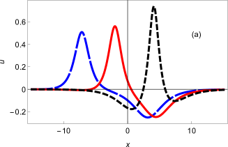
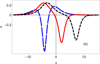
Figure 4: Details of the centre regions for the overtaking interaction, in part (a) of a smaller hole by a larger hump, for the parameters given in Figure 3(a), and in (b) of a smaller hump by a larger hole, for the parameters given in Figure 3(b). The curve coding is as in Figure 2.

The parameters are as in Figure 3, but with smaller time steps, for $t=-5,0,5$.

In particular, note that in part (a) the hole is split in two when the hump passes through, and the holes are less deep, rendering the hump larger. The net result is that the hole is transferred from being ahead of the hump to trailing it. On the other hand, in case (b) the hump is split when the hole passes through, with similar remarks about smaller humps and a deeper hole.

This mechanism has been observed in a variety of other parameter ranges we have investigated, but omitted here to avoid repetitive figures that are qualitatively similar. And, as before, the mechanism occurs for all ratios $|k_{1}/k_{2}|$.

The analogy between parts (a) and (b) of Figure 3 is due to an underlying antisymmetry:

$$u(-x,-t)\big{|}_{k_{1}\to-k_{1},\,k_{2}\to-k_{2}}=-u(x,t).$$ (16)

A consequence is that one can prove mathematically from (15) that $k_{1}+k_{2}\to 0$ yields $u(x,t)\to 0$. This is to be anticipated: When the hole is as deep as the hump is tall, both will cancel and travel at the same speed, hence one is reduced to the trivial solution of the mKdV equation.

5 Electric field profiles

We recall that $u=\varphi_{1}$ represents the electrostatic potential. In the theoretical analysis of acoustic solitons in multispecies plasmas this is usually the more important quantity. However, its derivatives have a physical meaning: up to a change of sign, the first derivative gives the electric field, and the second, the global charge density of the plasma. This is in contrast to the original application of the KdV equation – describing solitary waves on the surface of shallow water – where the height of the wave is important but the derivatives of that elevation are not of physical interest.

In plasma applications, the electric field of the wave is given by

$$E=-\frac{\partial{\varphi}}{\partial{x}}.$$ (17)

With respect to solitary waves having a potential hump or hole, it follows that the associated electric fields show a typical bipolar signature, of which a generic picture is given in Figure 5 for a positive single-soliton solution (5).

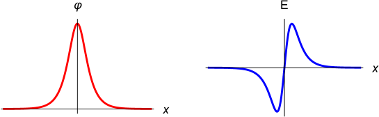
Figure 5: Generic profiles for mKdV single-soliton solution and associated electric field.

For a potential hump, where the electrostatic potential rises from zero to a maximum, before decreasing again to zero at infinity, its derivative is initially positive but then switches to negative. Because of the minus sign in the definition of the electric field, the bipolar structure starts with a negative part and ends with a positive part. For potential holes the opposite occurs. Thus, the electric field is also an indicator for the polarity of the mode.

The interest in such bipolar electric field structures stems from the fact that they have been observed in a plethora of space observations by ionospheric and auroral satellite missions as diverse as GEOTAIL [Matsumoto et al. (1994)], POLAR [Franz et al. (1998, 2005)], FAST [McFadden et al. (2003)] and CLUSTER [Pickett et al. (2004, 2008); Norgren et al. (2015)] where the electric field (rather than the electrostatic potential) is observed. In some of the satellite observations both the electrostatic potential and the electric field are observed by different instruments [McFadden et al. (2003)], which can thus serve as a way to check the consistency of the observations.

However, there are many different ways of modelling such structures, which in the case of electron holes refer to a localized plasma region where the electron density is lower than the surrounding plasma [Hutchinson (2017)]. The decreased electron density causes a local maximum in charge density and electrostatic potential. They might be viewed as a Bernstein-Greene-Kruskal (BGK) mode [Bernstein et al. (1957)], but can also be described in terms of solitons. For further details we refer to an excellent overview by Hutchinson (2017) and to recent extensions of BGK theory by Harikrishnan et al. (2018a, b). Among the many interpretations, the one that interests us here is that of electrostatic solitary waves and structures, but there remains ambiguity in identifying the nature of observed phenomena.

Furthermore, there are many observations that do not fit the simple patterns and cannot be explained by simple solitons and their electric fields. A specific example is found in Figure 1(b) in [Pickett et al. (2004)], where besides the typical bipolar structures there are tripolar structures or modifications of the bipolar electric field structure by wiggles on the sides. For the latter we advanced a possible explanation in terms of supersolitons [Dubinov & Kolotkov (2012); Verheest et al. (2013); Verheest & Hellberg (2015); Kakad et al. (2016); Olivier et al. (2018)], but in personal correspondence with the lead author of Pickett et al. (2004) these were thought to indicate an overtaking or even merging of solitons [Pickett (2013)].

Moreover, in most of the observed electric fields, the bipolar profiles have larger or smaller amplitudes, which – if they are due to propagating solitons – implies that the smaller ones will be overtaken by the larger ones. The property that larger amplitude structures are faster than smaller ones also holds for large amplitude solitary waves [Verheest (2010)] which are commonly described by a Sagdeev pseudopotential formalism [Sagdeev (1966)]. The drawback of this method is that it usually does not give analytical expressions for the profiles nor for their interactions. Outside the KdV range, results will have to come from numerical simulations (see, e.g., Kakad et al. (2017)).

Of course, observing the precise overtaking of two bipolar structures would be serendipitous, but signals close to or after an overtaking collision have been recorded. Regardless of their theoretical explanation, these observations have been interpreted in terms of propagating structures, even though that has rarely been unambiguously confirmed. There are some CLUSTER observations where a fortuitous configuration of two of the four satellites was able to capture propagation of the major structures, while others were already quite distorted [Pickett et al. (2008); Norgren et al. (2015)].

Hence, in what follows we focus on the interaction properties of the electric fields. The graphs to follow show the negative of the derivative of (15) with respect to $x$. We omit the cumbersome mathematical expression of the derivative because it offers no physical insight. Using the same parameter conditions as in Figures 1–4, we start with the positive electrostatic polarities in Figure 6.

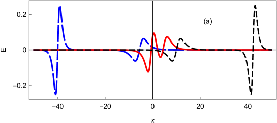
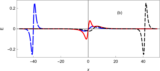
Figure 6: Electric field profiles of the soliton interactions for (a) $k_{1}=0.5$ or (b) $k_{1}=0.3$ and $k_{2}=1$, as shown in Figure 1. The curves correspond to $t=-40,0,40$, with a similar curve coding.

As in Figure 1, the parameters determining the respective shapes of the solitons are (a) $k_{1}=0.5$ and (b) $k_{1}=0.3$, both with $k_{2}=1.$ The curves are shown for $t=-40,0,40$ with the usual curve coding. Far away from the interaction region, the electric field shows two characteristic bipolar signatures, a stronger one for the larger soliton and a weaker one for the smaller soliton.

As can be seen on these graphs, during the interaction the curves become quite muddled. This is shown in more detail in Figure 7, for both sets of parameters.

  

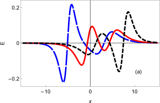
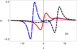
Figure 7: Details of the electric field profiles for the parameters used in Figure 6. The curves correspond to $t=-5,0,5$.

Parts (a) of Figures 1 and 2 showed two distinct peaks. Parts (b) of the same figures illustrated that the peaks briefly merged into a single distorted one. Consequently, in Figures 6 and 7 there are always two distinct bipolar signatures in parts (a), sometimes very close together, whereas in parts (b) there is a stage when there is only one bipolar structure, but with wiggles on the wings. Some of the latter characteristics have also been seen on supersolitons, but in larger-amplitude descriptions outside the reductive perturbation approach [Dubinov & Kolotkov (2012); Verheest et al. (2013)] or in simulations [Kakad et al. (2016)].

Next, in Figures 8 and 9 we graph the overtaking of a smaller hole by a larger hump.

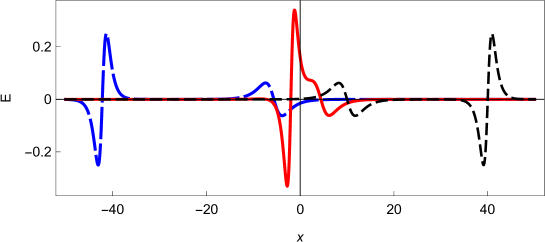
Figure 8: Electric field profiles for $k_{1}=-0.5$ and $k_{2}=1$ for the soliton interactions shown in Figure 3.

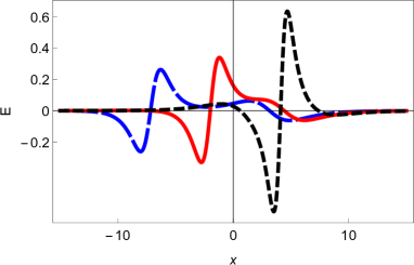
Figure 9: Details of the electric field profiles for the parameters used in Figure 8. The curves correspond to $t=-5,0,5$.

Here again, the electric field bipolar signatures can be recognized far from the interaction zone, except that now the signatures differ not only in amplitude but also in sign. This is less often seen in space observations but the complicated interaction region itself might perhaps help with identifying new features.

The figures for the converse case, i.e., the overtaking of a smaller hump by a larger hole, would be obtained by flipping the graphs shown in Figures 8 and 9 over the $x$ axis (not shown).

The second derivative of $u=\varphi$ also has a physical interpretation. Indeed, it follows from Poisson’s equation

$$\sigma=-\frac{\partial{{}^{2}\varphi}}{\partial{x^{2}}}$$ (18)

that, up to a sign, it corresponds to the global charge density in the solitary wave(s). However, this has rarely been plotted in theoretical papers. Viewed more as a curiosity than for its additional physical insight, the available plots are only for single solitons or double layers [Verheest & Hellberg (2015)]. Due to the additional local extrema, we have not attempted to graph these density curves for two interacting mKdV solitons.

6 Conclusions

While many papers have covered two-soliton overtaking interactions in plasmas, they have mostly focused on KdV solitons having the same polarity. We stress that the KdV equation can only deal with one sign of the quadratic nonlinearity for a given model. Likewise, mKdV equations can address the overtaking of same polarity solitons, in which case profiles and interaction regions look quite similar to what one obtains for KdV solitons. Depending on the relative amplitudes (or equivalently, velocities), the salient feature for two-soliton interaction of the same polarity is that there are either always two distinct humps or that they briefly merge in the interaction region into a single distorted hump. In either case, the collisions are accompanied by phase shifts.

The most interesting case is the overtaking of mKdV solitons of opposite polarities, where in the interaction region the slower soliton slows down and splits, to let the faster soliton pass through. While this happens, the faster soliton is temporarily slightly accelerated. Far from the interaction region, on either side, the solitons are well separated and each matches the sech-profile of a single mKdV soliton.

Relevant to plasma physics is the study of the associated electric fields, which are often seen in ionospheric and magnetospheric satellite observations. Seemingly, the electric fields are more easily observed than the electrostatic solitons themselves. Such electric fields are characterized by typical bipolar structures or variations thereof. In this paper we discussed and illustrated the overtaking and interaction properties of some of these signatures. As far as we know, this is a novel application.

The case of opposite polarity modes overtaking each other is more rare. It might therefore be interesting to search for some of these in more complicated scenarios, in particular, where not all signatures are purely bipolar and well separated.

References

- Ablowitz & Clarkson (1991) Ablowitz, M. J. and Clarkson, P. A. 1991 Solitons, Nonlinear Evolution Equations and Inverse Scattering (Cambridge University Press. U.K.).
- Anco et al. (2011) Anco, S. C., Ngatat, N. T. and Willoughby, M. 2011 Interaction properties of complex modified Korteweg-de Vries (mKdV) solitons. Physica D 240, 1378–1394.
- Bernstein et al. (1957) Bernstein, I. B., Greene, J. M. and Kruskal, M. D. 1957 Exact nonlinear plasma oscillations. Phys. Rev. 108, 546–550.
- Cairns et al. (1995) Cairns, R. A., Mamun, A. A., Bingham, R., Boström, R, Dendy, R. O., Nairn, C. M. C. and Shukla, P. K. 1995 Electrostatic solitary structures in non-thermal plasmas. Geophys. Res. Lett. 22, 2709–2712.
- Das (1975) Das, G. C. 1975 Ion-acoustic solitary waves in multicomponent plasmas with negative-ions. IEEE Trans. Plasma Sci. 3, 168–173.
- Das & Tagare (1975) Das, G. C. and Tagare, S. G. 1975 Propagation of ion-acoustic waves in a multi-component plasma. Plasma Phys. 17, 1025–1032.
- Drazin & Johnson (1989) Drazin, P. G. and Johnson, R. S. 1989 Solitons: An Introduction (Cambridge University Press, U.K.).
- Dubinov & Kolotkov (2012) Dubinov, A. E. and Kolotkov, D. Yu. 2012 Ion-acoustic super solitary waves in dusty multispecies plasmas, IEEE Trans. Plasma Sci. 40, 1429–1433.
- Franz et al. (1998) Franz, J. R., Kintner, P. M. and Pickett, J. S. 1998 POLAR observations of coherent electric field structures. Geophys. Res. Lett. 25, 1277–1280.
- Franz et al. (2005) Franz, J. R., Kintner, P. M., Pickett, J. S. and Chen, L.-J. 2005 Properties of small-amplitude electron phase-space holes observed by Polar. J. Geophys. Res. 110, A09212.
- Gardner et al. (1967) Gardner, C. S., Greene, J. M., Kruskal, M. D. and Miura, R. M. 1967 Method for solving the Korteweg-de Vries equation. Phys. Rev. Lett. 19, 1095–1097.
- Gardner et al. (1974) Gardner, C. S., Greene, J. M., Kruskal, M. D. and Miura, R. M. 1974 Korteweg-de Vries equations and generalizations: methods for exact solutions. Comm. Pure Appl. Math. 27, 97–133.
- Harikrishnan et al. (2018a) Harikrishnan, A., Kakad, A. and Kakad, B. 2018a Bernstein-Greene-Kruskal theory of electron holes in superthermal space plasma. Phys. Plasmas 25, 052901.
- Harikrishnan et al. (2018b) Harikrishnan, A., Kakad, A. and Kakad, B. 2018a Effects of wave potential on electron holes in thermal and superthermal space plasmas. Phys. Plasmas 25, 122901.
- Harvey et al. (2010) Harvey, P., Durniak, C., Samsonov, D. and Morfill, G. 2010 Soliton interaction in a complex plasma. Phys. Rev. E 81, 057401.
- Hirota (1971) Hirota, R. 1971 Exact solution of the Korteweg-de Vries equation for multiple collisions of solitons. Phys. Rev. Lett. 27, 1192–1194.
- Hirota (1972) Hirota, R. 1972 Exact solution of the modified Korteweg-de Vries equation for multiple collisions of solitons. J. Phys. Soc. Japan 33, 1456–1458.
- Hirota (2004) Hirota, R. 2004 The Direct Methods in Soliton Theory (Cambridge University Press, U.K.).
- Hutchinson (2017) Hutchinson, I. H. 2017 Electron holes in phase space: What they are and why they matter, Phys. Plasmas 24, 055601.
- Kakad et al. (2016) Kakad, A., Lotekar, A. and Kakad, B. 2016 First-ever model simulation of the new subclass of solitons “Supersolitons” in plasma. Phys. Plasmas 23, 110702.
- Kakad et al. (2017) Kakad, A., Kakad, B. and Omura, Y. 2017 Formation and interaction of multiple coherent phase space structures in plasma. Phys. Plasmas 24, 060704.
- Korteweg & de Vries (1895) Korteweg, D. J. and de Vries, G. 1895 On the change of form of long waves advancing in a rectangular canal, and on a new type of long stationary waves. Philos. Mag. 39, 422–443.
- Kumar et al. (2017) Kumar, S., Kumar Tiwari, S. and Das, A. 2017 Observation of the Korteweg-de Vries soliton in molecular dynamics simulations of a dusty plasma medium. Phys. Plasmas 24, 033711.
- Lee (2009) Lee, N. C. 2009 Small amplitude electron-acoustic double layers and solitons in fully relativistic plasmas of two-temperature electrons. Phys. Plasmas 16, 042316.
- Lima et al. (2000) Lima, J. A. S., Silva, Jr., R. and Santos, J. 2000 Plasma oscillations and nonextensive statistics. Phys. Rev. E 61, 3260–3263.
- Matsumoto et al. (1994) Matsumoto, H., Kojima, H., Miyatake, T., Omura, Y., Okada, M., Nagano, I. and Tsutsui, M. 1994 Electrostatic solitary waves (ESW) in the magnetotail: BEN wave forms observed by GEOTAIL. Geophys. Res. Lett. 21, 2915–2918.
- McFadden et al. (2003) McFadden, J. P., Carlson, C. W., Ergun, R. E., Mozer, F. S., Muschietti, L., Roth, I. and Moebius, E. 2003 FAST observations of ion solitary waves. J. Geophys. Res. 108, (A4) 8018, doi:10.1029/2002JA009485.
- Nakamura & Tsukabayashi (2009) Nakamura, Y. and Tsukabayashi, I. 2009 Modified Korteweg—de Vries ion-acoustic solitons in a plasma. J. Plasma Phys. 34, 401–415.
- Norgren et al. (2015) Norgren, C., André, M., Vaivads, A. and Khotyaintsev, Y. V. 2015 Slow electron phase space holes: Magnetotail observations. Geophys. Res. Lett. 42, 1654–1661.
- Olivier et al. (2018) Olivier, C. P., Verheest, F. and Hereman, W. A. 2018 Collision properties of overtaking supersolitons with small amplitudes. Phys. Plasmas 25, 032309.
- Pickett et al. (2004) Pickett, J. S., Chen, L.-J., Kahler, S. W., Santolík, O., Gurnett, D. A., Tsurutani, B. T. and Balogh, A. 2004 Isolated electrostatic structures observed throughout the Cluster orbit: relationship to magnetic field strength. Annales Geophys. 22, 2515–2523.
- Pickett et al. (2008) Pickett, J. S., Chen, L.-J., Mutel, R. L., Christopher, I. W., Santolík, O., Lakhina, G. S., Singh, S. V., Reddy, R. V., Gurnett, D. A., Tsurutani, B. T., Lucek, E. and Lavraud, B. 2008 Furthering our understanding of electrostatic solitary waves through Cluster multispacecraft observations and theory. Adv. Space Res. 41, 1666–1676.
- Pickett (2013) Pickett, J. S. 2013 Private communication.
- Sagdeev (1966) Sagdeev, R. Z. 1966 Cooperative phenomena and shock waves in collisionless plasmas. Reviews of Plasma Physics, ed. by M. A. Leontovich (Consultants Bureau, New York), Vol. 4, pp. 23–91.
- Saini & Shalini (2013) Saini, N. S. and Shalini (2013) Ion acoustic solitons in a nonextensive plasma with multi-temperature electrons. Astrophys. Space Sci. 346, 155–163.
- Summers & Thorne (1991) Summers, D. and Thorne, R. M. 1991 The modified plasma dispersion function. Phys. Fluids B 3, 1835–1847.
- Tagare (1986) Tagare, S. G. 1986 Effect of ion-temperature on ion-acoustic solitons in a two-ion warm plasma with adiabatic positive and negative ions and isothermal electrons. J. Plasma Phys. 36, 301–312.
- Tsallis (1988) Tsallis, C. 1988 Possible generalization of Boltzmann-Gibbs statistics. J. Stat. Phys. 52, 479–487.
- Vasyliunas (1968) Vasyliunas, V. M. 1968 A survey of low-energy electrons in the evening sector of the magnetosphere with OGO 1 and OGO 3. J. Geophys. Res. 73, 2839–2884.
- Verheest (1988) Verheest, F. 1988 Ion-acoustic solitons in multi-component plasmas including negative ions at critical densities. J. Plasma Phys. 39, 71–79.
- Verheest (2000) Verheest, F. 2000 Waves in Dusty Space Plasmas (Kluwer Academic, Dordrecht, The Netherlands) pp. 109–112.
- Verheest (2010) Verheest, F, 2010 Nonlinear acoustic waves in nonthermal dusty or pair plasmas. Phys. Plasmas 17, 062302.
- Verheest (2015) Verheest, F. 2015 Critical densities for KdV-like acoustic solitons in multi-ion plasmas. J. Plasma Phys. 81, 905810605.
- Verheest & Hellberg (2015) Verheest, F. and Hellberg, M. A. 2015 Electrostatic supersolitons and double layers at the acoustic speed, Phys. Plasmas 22, 012301.
- Verheest et al. (2012a) Verheest, F., Hellberg, M. A. and Hereman, W. A. 2012a Head-on collisions of electrostatic solitons in nonthermal plasmas. Phys. Rev. E 86, 036402.
- Verheest et al. (2012b) Verheest, F., Hellberg, M. A. and Hereman, W. A. 2012b Head-on collisions of electrostatic solitons in multi-ion plasmas. Phys. Plasmas 19, 092302.
- Verheest et al. (2013) Verheest, F., Hellberg, M. A. and Kourakis, I. 2013 Electrostatic supersolitons in three-species plasmas, Phys. Plasmas 20, 012302 (2013).
- Watanabe (1984) Watanabe, S. 1984 Ion acoustic soliton in plasma with negative ions. J. Phys. Soc. Jpn. 53, 950–956.
- Zabusky & Kruskal (1965) Zabusky, N. J. and Kruskal, M. D. 1965 Interactions of solitons in a collsionless plasma and the recurrence of initial states. Phys. Rev. Lett. 15, 240–243.