Cosmic Pathways for Compact Groups in the Milli-Millennium Simulation

Abstract

We detected 10 compact galaxy groups (CGs) at $z=0$ in the semianalytic galaxy catalog of Guo et al. (2011) for the milli-Millennium Cosmological Simulation (sCGs in mGuo2010a). We aimed to identify potential canonical pathways for compact group evolution and thus illuminate the history of observed nearby compact groups. By constructing merger trees for $z=0$ sCG galaxies, we studied the cosmological evolution of key properties, and compared them with $z=0$ Hickson CGs (HCGs). We found that, once sCG galaxies come within 1 (0.5) Mpc of their most massive galaxy, they remain within that distance until $z=0$, suggesting sCG “birth redshifts.” At $z=0$ stellar masses of sCG most massive galaxies are within $10^{10}\lesssim M_{\ast}/M_{\odot}\lesssim 10^{11}$. In several cases, especially in the two four- and five-member systems, the amount of cold gas mass anticorrelates with stellar mass, which in turn correlates with hot gas mass. We define the angular difference between group members’ 3D velocity vectors, $\Delta\theta_{\rm vel}$, and note that many of the groups are long-lived because their small values of $\Delta\theta_{\rm vel}$ indicate a significant parallel component. For triplets in particular, $\Delta\theta_{\rm vel}$ values range between $20\degr$ and $40\degr$ so that galaxies are coming together along roughly parallel paths, and pairwise separations do not show large pronounced changes after close encounters. The best agreement between sCG and HCG physical properties is for $M_{\ast}$ galaxy values, but HCG values are higher overall, including for star formation rates (SFRs). Unlike HCGs, due to a tail at low SFR and $M_{\ast}$, and a lack of $M_{\ast}$ $\gtrsim 10^{11}$ $M_{\odot}$ galaxies, only a few sCG galaxies are on the star-forming main sequence.

Key words: galaxies: evolution – galaxies: groups: general – galaxies: interactions

2019 February 5

1 Introduction

As their name implies, compact groups of galaxies (CGs) constitute a distinct class of galaxy systems, consisting of agglomerations of just a few galaxies, typically separated by a few galaxy radii (median projected separations of $\sim 40\ h^{-1}$ kpc, where $h\equiv H_{0}/100$ and $H_{0}$ is the Hubble constant at $z=0$). Their low galaxy velocity dispersions (radial median of $\sim$200 km s^-1), combined with high galaxy number densities (up to $10^{8}h^{2}\,\rm Mpc^{-2}$; Hickson, 1982; Hickson et al., 1992), make them an environment favoring strong and prolonged galaxy interactions. Understanding galaxy evolution in CGs is of great interest, as most galaxies spend the majority of their time in some type of group environment (Mulchaey, 2000; Karachentsev, 2005, and references therein).

Since the compilation of dedicated observational CG catalogs more than 30 years ago (Rose, 1977; Hickson, 1982), it has become clear that galaxies in the CG environment show characteristics that are distinct compared to virtually all other extragalactic environments, including field galaxies, isolated pairwise mergers, and galaxy clusters (Johnson et al., 2007; Tzanavaris et al., 2010; Walker et al., 2010, 2012; Lenkić et al., 2016; Zucker et al., 2016), with the notable exception of the Coma Cluster outskirts (Walker et al., 2010, 2012). CG galaxies show a “canyon” in mid-infrared (MIR) color space, suggestive of a rapid transition from actively star-forming to quiescent systems, although most CG galaxies reside in the optical “red sequence” rather than the “green valley” (Walker et al., 2013; Zucker et al., 2016). Consistent with the latter observation, and compared to loose groups and field galaxies, late-type CG galaxies have overall markedly reduced stellar-mass normalized star formation rates (SFRs) (“specific” SFRs [sSFRs]; Coenda et al. 2015) and a higher fraction of quiescent galaxies that are not actively forming stars (Coenda et al., 2015; Lenkić et al., 2016). Tzanavaris et al. (2016) found that, compared to general correlations established for late-type galaxies in the local universe (e.g., Mineo et al., 2012), many of these late-type galaxies exhibit a pronounced excess in X-ray luminosity from high-mass X-ray binaries for their SFR. The MIR canyon is further consistent with an observed bimodality in sSFRs, which is essentially exclusive to CGs (Tzanavaris et al., 2010; Lenkić et al., 2016), with some similar behavior observed in loose galaxy groups (Wetzel et al., 2012). Further, by studying warm H₂, Alatalo et al. (2015) also observed bimodal suppression of star formation (see also Cluver et al., 2013).

CG galaxies tend to have older stellar populations on average (Proctor et al., 2004; Mendes de Oliveira et al., 2005; Coenda et al., 2015). Compared to loose groups, they correspondingly show a larger fraction of red and early-type systems (Coenda et al., 2012). Their brightest group galaxies are more luminous, more massive, larger, redder, and are more frequently classified as ellipticals than the other galaxies in the groups (Martínez et al., 2013).

Overall, these features of CGs compared to other environments imply that the CG environment affects member galaxy evolution in a unique way, possibly linked to pronounced interaction activity that is likely to be occurring, or has occurred in the past, in these systems (see the Fabry-Pérot work in Plana et al., 1998; Mendes de Oliveira et al., 1998, 2003; Amram et al., 2004; Torres-Flores et al., 2009, 2010, 2014).

For the most part, observed CGs (e.g., Hickson et al., 1992; Barton et al., 1996; Lee et al., 2004; Deng et al., 2007; McConnachie et al., 2009; Díaz-Giménez et al., 2012) only allow us to study the effects of the CG environment in the relatively nearby universe. For instance, the Redshift Survey Compact Group catalog (Barton et al., 1996) reaches $m_{B}<15.5$ and $z\lesssim 0.03$. The advent of cosmological simulations in the past few decades has provided a novel way to probe the evolution of structure in the universe by comparing observations with simulations. In the case of CGs, one can compare observations with simulations at $z=0$ to identify simulated systems that may resemble observed ones. With the information from the simulation database in hand, one can then look backward in time along the merger trees of the “best-fit” simulated systems and learn about plausible evolutionary histories for individual CGs.

A number of studies have used galaxy catalogs derived from the dark matter Millennium Simulation (Springel et al., 2005) to study CGs. McConnachie et al. (2008) used a mock galaxy catalog derived using the code of Blaizot et al. (2005) from the De Lucia & Blaizot (2007) semianalytic galaxy catalogs. They identified mock CGs in projection in the Millennium Simulation and compared them to observed Hickson CGs (HCGs), finding that about a third of the mock CGs are truly physically dense systems of three or more galaxies, while the remaining are chance alignments. Díaz-Giménez & Mamon (2010) further explored the origin of this issue, finding fractions of physically dense systems between 20% and 45%, depending on the semianalytic galaxy catalog used. On the other hand, Díaz-Giménez & Zandivarez (2015) compared CGs from the 2MASS catalog to those in the Henriques et al. (2012) mock light cone, whose galaxy properties were produced via the Guo et al. (2011) semianalytic model. They found that about two-thirds of CGs are truly isolated and not part of larger structures. Snaith et al. (2011) used four semianalytic models to compare the predicted luminosity distribution of both loose and compact groups among different models and observations. In spite of some agreement with observations, they found clear differences between semianalytic models. Farhang et al. (2017) used the De Lucia & Blaizot (2007) semianalytic galaxy catalog of the Millennium Simulation to compare the mass assembly histories of compact and fossil groups. They found no strong evidence that CGs are part of a general evolutionary group path that leads to the eventual formation of fossil groups. They concluded that CGs should instead constitute a specific class of groups with a distinct evolutionary path.

In this paper, we take an alternative approach and look for small systems of galaxies that are physically close in 3D space, rather than apparently close in a 2D projection that approximates an astronomical image. In addition, we use a subset of the galaxy catalog of Guo et al. (2011) known as the milli-Millennium simulation. We refer to this subset of the catalog as mGuo2010a and use it to search for CGs forming in the simulation by means of a clustering algorithm to identify small systems of galaxies in physically close proximity that are also isolated. We stress that, because the volume of the simulation is very small (only 1/512 of the full Millennium Simulation volume), we are not looking for statistical samples and patterns. Instead, we are examining in detail the small number of simulation compact groups (sCGs) in mGuo2010a and following the evolution of their individual components through space and time. We then compare the properties of the simulated galaxies at $z=0$ with well-known CG members observed in the local universe to look for the best matches. The aim is to search for evolutionary analogs to elucidate the possible histories of observed CGs. Rather than making any sweeping claims on CG formation and evolution as a whole, we simply treat the sCGs as interesting “case studies” to help establish and explore the potential parameter space of CG histories and set up future studies.

The structure of the paper is as follows: Section 2 describes our strategy and algorithm for identifying CGs in the simulation, visualization, and results, including key properties of identified systems. Section 3 compares mGuo2010a-detected sCGs to observed HCGs. Section 4 discusses our findings. The paper concludes with a summary in Section 5. Consistent with the Millennium Simulation, we make use of cosmological parameters $H_{0}=73\ {\rm km}\ {\rm s}^{-1}\ {\rm Mpc}^{-1}$, $\Omega_{M}=0.25$, and $\Omega_{\Lambda}=0.75$ throughout. This is also consistent with observational results from the Carnegie Hubble Program (Freedman et al., 2012), as well as the WMAP (Hinshaw et al., 2013) mission.

2 Compact Groups in the Guo et al. (2011) Catalog of the Milli-Millennium Simulation

2.1 Simulation

The Millennium Cosmological Simulation (Springel et al., 2005) is one of the best-known high-performance computing simulations tracing the evolution of dark matter structure over cosmic time. It was one of the first computer simulations that provided us with a detailed look at the universe at large scales while still being able to resolve structures smaller than the size of individual galaxies. The simulation used $2160^{3}$ particles of mass $8.6\times 10^{8}\ h^{-1}\ M_{\odot}$ inside a comoving cube $500\ {\rm Mpc}\ h^{-1}$ on a side. It traces the evolution of this cube in 64 redshift snapshots between $z=127$ and $z=0$, a range of approximately 13.56 Gyr in cosmic time. Figure 1 displays a snapshot of a section of the Millennium Simulation at $z=0$.

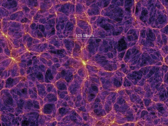
Figure 1: Snapshot of the projected dark matter density field for a $15\ {\rm Mpc}\ h^{-1}$ thick slice of the Millennium Simulation at $z=0$ (Springel et al., 2005). The $125\ {\rm Mpc}\ h^{-1}$ scale bar indicates twice the length of the milli-Millennium Simulation box.

To compare with observed galaxies, dark matter halos are first identified in the simulations, and subsequently baryonic galaxies with their associated properties are assigned to them by means of semianalytic techniques (e.g., De Lucia & Blaizot, 2007; Guo et al., 2010, 2011, 2013, for the Millennium Simulation). Guo et al. (2011) have applied their semianalytic method to produce galaxy catalogs associated with the full Millennium Simulation. A chunk of the volume in the full simulation is also available, namely, the milli-Millennium Simulation. This second catalog, mGuo2010a, is available for testing of analysis that can then be applied to the full simulation after successful verification. The smaller volume of this catalog is more appropriate for the particular clustering detection algorithm used in this paper. We are not searching for statistical samples that would require the full Millennium Simulation volume, but rather interesting individual case studies that allow us to investigate diverse samples of CG evolution over time.

The milli-Millennium Simulation contains information for the same redshift snapshots as the full simulation but in a cube $62.5\ {\rm Mpc}\ h^{-1}$ on a side, resulting in a volume approximately $1/512$ that of the full simulation. Many well-studied HCGs are located within 60 Mpc of the Milky Way. Therefore, within a volume of this size, one would expect to find examples in the simulation that are similar to observed CGs if the simulation reasonably represents our universe and the volume around the Local Group is not unusual.

cccccMccccM[ht] Milli-Millennium Simulation Compact Groups      ID               $M_{*,\ z=0}$         $M_{{\rm CGas},\ z=0}$         $M_{{\rm HGas},\ z=0}$          SFR_z=0          $\Delta D_{\rm A}$ $\leqslant\ 1\,~{}\rm Mpc$          $\Delta D_{\rm A}$ $\leqslant\ 500\,~{}\rm kpc$      

     

$z$ Lifetime $z$ Lifetime $\langle\rm SFR\rangle$

 
$\log(M_{\odot})$ $\log(M_{\odot}$ ${\rm yr}^{-1})$ (Gyr) (Gyr) $\log(M_{\odot}$ ${\rm yr}^{-1})$
(1) (2) (3) (4) (5) (6) (7) (8) (9) (10) (11) 115 & Total 10.95 9.41 11.91 -2.48 0.91 7.20 0.41 4.23    0.02
A 10.84 8.44 11.90 …
B 10.10 9.10   9.53 …
C   9.94 9.00   7.86 -2.48
377 Total 11.12 9.89 11.93 -1.15 1.17 8.25 0.69 6.10    0.36
A 10.94 9.08 11.93 …
B 10.29 9.28   7.86 -2.30
C 10.04 9.30   6.37 -1.24
D   9.92 9.39   9.41 -2.13
E   9.80 8.34   7.48 …
518 Total   9.23 9.49   8.78 -1.18 3.06 11.41 1.39 8.90 -0.44
A   8.82 9.25   7.86 …
B   8.79 8.93   8.56 -1.63
C   8.61 8.69   8.21 -1.36
1056 Total 10.78 9.57 11.50 -0.95 0.62 5.73 0.09 1.13 -0.21
A 10.64 8.19 11.50 …
B 10.16 9.04   7.86 -1.64
C   9.27 9.39   9.08 -1.05
1119 Total 10.71 9.84 11.27    0.16 0.99 7.60 0.41 4.23    0.23
A 10.47 9.12 11.25 …
B 10.13 9.45   7.86 -1.79
C   9.93 9.44   9.94    0.16
1441 Total 10.76 9.83 11.51 -1.13 0.99 7.60 0.36 3.86 -0.63
A 10.59 9.42 10.09 -2.54
B 10.21 9.53 11.49 -1.15
C   9.36 8.90   7.86 -3.86
1598 Total 11.01 9.67 11.92 -0.16 0.62 5.73 0.17 2.09    0.51
A 10.87 8.48 11.92 …
B 10.15 9.36   8.22 -0.16
C 10.10 9.25   7.86 -3.20
D   9.40 8.51   8.06 …
1757 Total 10.69 9.06 11.29    0.62 1.17 8.25 0.28 3.13 -0.27
A 10.52 8.36 11.29    0.61
B 10.13 8.28   6.38 -2.04
C   9.24 8.85   8.83 -0.88
1773 Total   9.89 9.76 10.85 -0.32 2.62 11.01 0.83 6.84    0.41
A   9.77 9.63 10.85 -0.33
B   8.86 8.94   7.86 -2.21
C   9.10 8.81   7.86 -2.82
2143 Total 10.27 9.70 11.02 -0.26 1.77 9.78 0.36 3.86    0.01
A 10.17 9.40 11.01 …
B   9.33 9.02   9.01 -0.55
C   9.23 9.14   7.86 -0.58
Note. Member galaxy properties at $z=0$ for CGs identified with clues in the Guo2010a milli-Millennium database (sCGs; Guo et al., 2011, mGuo2010a). Column (1): sCG ID. Column (2): member galaxy ID (A to E, according to decreasing stellar mass). Column (3): stellar mass. Column (4): cold gas mass. Column (5): hot gas mass. Column (6): star formation rate. Column (7): redshift at which members of compact group come within $\Delta D_{\rm A}$ $\leqslant 1$ Mpc of the most massive galaxy for the first time. Column (8): lifetime as a compact group from aforementioned redshift to $z=0$. Columns (9)-(10): same as Columns (7)-(8), but instead using $\Delta D_{\rm A}$ $\leqslant 500$ kpc. Column (11): mean star formation rate during lifetime within $\leqslant 500$ kpc. In Column (6), where there are no entries, the Guo2010a semianalytical model assigns values of zero.

2.2 Detections with the clues Algorithm

The CLUstEring with local Shrinking (clues)package (Wang et al., 2007; Chang et al., 2010) is part of the R statistical software environment (R Core Team, 2012). It is a cluster analysis algorithm aiming to make minimal assumptions about datasets and an optimal identification of cluster numbers. clues is thus an unsupervised clustering analysis algorithm, where in particular the number of clusters is not an input value provided by the user. This is a major advantage for the type of analysis performed in this paper, where the number of clusters is not known in advance.

Briefly, clues identifies cluster centers by effectively drawing data points together (“shrinking”) until they converge on the cluster center, similarly to the behavior of point-mass particles in a gravitational field. In each iteration, the median position of all points in the smallest sphere containing $K$ nearest neighbors replaces all previous positions in the sphere until the distance $d$ between points in successive iterations becomes smaller than a stopping criterion $\epsilon$. Individual data points are then assigned to specific clusters (a process called “partitioning”) by successively calculating pairwise distances between neighboring points and identifying outliers in the distance distribution. The number $K$ is also iteratively optimized. Starting with a small $K$, its value is increased until one of two well-established indices of cluster strength are optimized, namely, Calinski and Harabsz (CH; Caliński & Harabasz 1974) or Silhouette (Rousseeuw, 1987).

For this paper, we used the clues (2.15.2) implementation in R to detect galaxy concentrations similar to CGs in the milli-Millennium Simulation. The data points searched by clues were simply the 3D Euclidean coordinates of galaxies in the catalog. We restricted the search to $z=0$ and $M_{V}<-18$ to select against dwarf galaxies and mimic the Hickson (1982) compactness criterion. As the Silhouette index has proven more successful in identifying clusters with irregular shapes, we used this index as a measure of cluster strength. After completing the clues analysis, for each cluster we identified the minimum galaxy magnitude, $M_{V,{\rm min}}$, and then removed any galaxies with magnitudes $\geqslant M_{V,{\rm min}}+3$, mimicking the Hickson (1982) magnitude range. We calculated a radius, defined as the maximum distance between the cluster center and each member galaxy, as well as the separation from all other clusters. We discarded clusters that were separated from their nearest neighbor by less than three times their diameter, aiming to mimic in 3D the Hickson (1982) angular isolation criterion. Finally, clusters that had fewer than three galaxy members were also discarded, to match the standard observational practice for CGs.

The result of this process was a list of 12 galaxy groups, containing 41 galaxies at $z=0$ in mGuo2010a. Although the clues-based selection is in 3D space and thus not fully consistent with the selection of observed CGs, the identified systems are still isolated, compact galaxy concentrations, and we refer to them as simulated compact groups (sCGs). For two of these there were unphysical discontinuities in positional information along the merger trees, likely due to proximity to the edge of the simulation box. We could thus not reliably construct merger trees and discarded these systems.

Among the remaining 10 sCGs (Table 1), one had four members (sCG 1598), and one had five members (sCG 377). The remaining eight had three members.

2.3 Galaxy Properties and Visualization

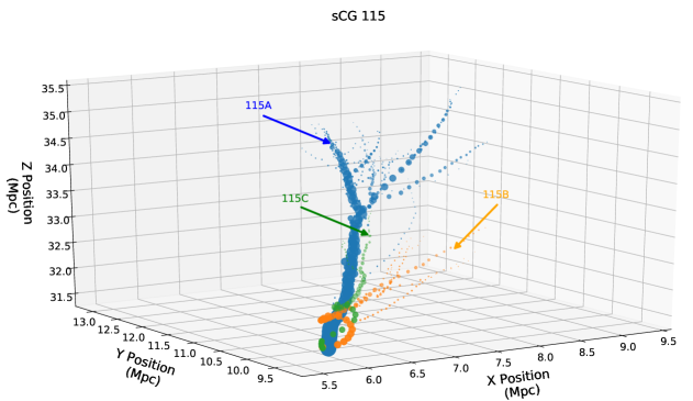
Figure 2: 3D merger tree for sCG 115, reconstructed from mGuo2010a data. Member galaxies are shown as filled colored circles, and circle sizes scale with $M_{\ast}$. Galaxies evolve from low to high $M_{\ast}$, and the final configuration of the group at $z=0$ is near the lower center of the figure as viewed in perspective. Galaxies are labeled A to C in order of decreasing $M_{\ast}$ at $z=0$.

We use the ID numbers assigned to identified sCGs by the clues algorithm. Strictly, these only apply to sCGs at $z=0$; however, for simplicity, we use them to refer to sCGs, as well as their past constituents, throughout their evolution over cosmic time along their merger trees (Lee et al., 2014). The merger tree information is extracted from the mGuo2010a database using the $z=0$ mGuo2010a galaxy IDs (preserved by clues). The mGuo2010a catalog contains information for 82 galaxy properties over the 64 redshift snapshots of the simulation. Apart from the redshift of each snapshot, we used SQL catalog queries to obtain information for 10 properties in each snapshot, namely, stellar mass ($M_{\ast}$), cold gas mass ($M_{\rm CGas}$), hot gas mass ($M_{\rm HGas}$), SFR, and $xyz$ positions and velocities.

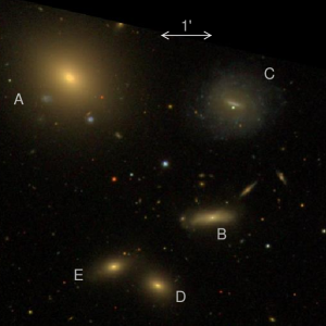
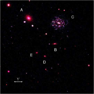
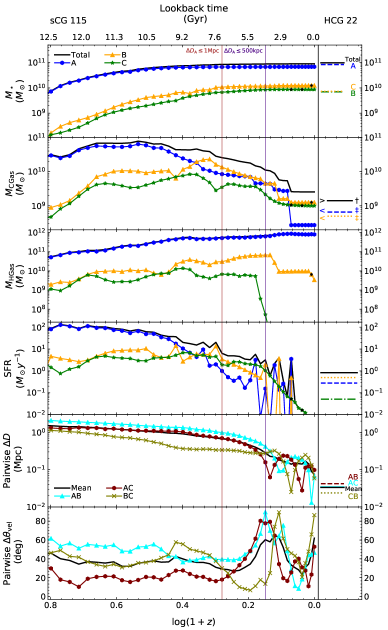
Figure 3: Top Left: SDSS $u,g,r,i,z$ optical image of HCG 22 (all SDSS images in this paper from https://skyserver.sdss.org/dr14/en/home.aspx). Bottom Left: Swift/UVOT three-band image of HCG 22, with blue, green, and red colors corresponding to the uvw2, uvm2, and uvw1 filters, respectively (Tzanavaris et al., 2010, and/or Swift archive for this and all Swift/UVOT images in this paper). Galaxies D and E are background objects. Right: from top to bottom, left hand panels show cosmic evolution of $M_{\ast}$, cold gas mass, hot gas mass, SFR, pairwise galaxy separation, and pairwise velocity vector angle for sCG 115. The top axis gives the corresponding look-back time, and the bottom axis gives the redshift. The color-coding for each galaxy of sCG 115 corresponds directly to that in the 3D merger tree shown in Figure 2. In each panel, the solid black line shows either the combined group total (for $M_{\ast}$, $M_{\rm CGas}$, $M_{\rm HGas}$, and SFR) or the mean (for pairwise $\Delta D$ and $\Delta\theta_{\rm vel}$). The brown vertical line across all panels indicates when CG members come within $\leqslant 1$ Mpc of the most massive galaxy for the first time, while the purple vertical line shows the same for $\leqslant 500$ kpc. In the galaxy separation panel, AB gives the separation between galaxies A and B, AC between galaxies A and C, etc. The color-coding and symbol coding for this panel also apply to the velocity vector angle panel. The black points indicate interpolated data points where data from the simulation were missing. Right hand panels show values for the same quantities as in the left hand panels but for HCG 22 galaxies at $z=0$ (Table 7), where available. In this case the HCG 22B and HCG 22C galaxies are not in order of decreasing stellar mass; the line color/style still reflects decreasing stellar mass, so that sCG 115B is matched with HCG 22C and sCG 115C with HCG 22B. The galaxy separations for HCGs are 2D projections and will therefore be underestimates.

For each sCG, we label member galaxies A through E by decreasing stellar mass at $z=0$. For five SCGs that show the greatest agreement in $M_{\ast}$ with observed groups (Section 3), we present visualizations of the merger trees and evolution of key properties in Figures 2, 3, 4, 5, 6, 7, 8, 9, 10 and 11. In the merger tree visualizations, each galaxy is indicated by a different filled colored circle throughout its evolutionary history that also includes mergers; merger constituents retain the $z=0$ galaxy color. Circle sizes scale with relative galaxy stellar mass.

Apart from the properties gleaned from the mGuo2010a catalog for individual galaxies, we also calculated two additional quantities. For each pair of sCG galaxies in each redshift snapshot, we calculated the pairwise Euclidean distance, $\Delta D$, between the galaxy positions in 3D space. We separately label $\Delta D_{\rm A}$ the distances between the galaxy with the most stellar mass, A, and other sCG member galaxies; for each sCG we identified the redshift snapshots where each galaxy (other than A) comes within $\Delta D_{\rm A}$ $\leqslant\ 1\ \rm{Mpc}$ and $\leqslant\ 500\ \rm{kpc}$ of the most massive group galaxy. The significance of this is discussed below. We also calculated angular separations of velocity vectors for all sCG member galaxy pairs across all snapshots. We defined these vectors for each galaxy by means of start- and end-position vectors for each look-back time snapshot interval. Over cosmic time these provide a quantitative characterization of the directional evolution of each galaxy’s path in 3D space. For each galaxy pair we thus obtained the evolution of the angle $\Delta\theta_{\rm vel}$ between the velocity vectors of the two galaxies by means of the cross product of the vectors. Due to merging, in $z>0$ snapshots a single $z=0$ galaxy may correspond to several precursors. In such cases $\Delta D$ and $\Delta\theta_{\rm vel}$ were calculated between the most massive galaxy precursors of the $z=0$ galaxies.

We present results for these key properties of individual sCG galaxies in Table 1. Specifically, in Columns (3) to (5) we show values for $M_{\ast}$, $M_{\rm CGas}$, and $M_{\rm HGas}$ both for member galaxies and the group as a whole for each sCG at $z=0$. Columns (7) and (9) give the redshift at which member galaxies come within $\Delta D_{\rm A}$ of 1 and 0.5 Mpc, respectively, of the most massive galaxy, A, for the first time. The significance of these particular values is that, once galaxies come this close, they remain within 1 (0.5) Mpc of A to $z=0$. Thus, these redshifts can be considered as fiducial points in cosmic time when the parent group is “born,” while these separations from galaxy A are in some sense two possible measures of a maximal “size” for a galaxy concentration to be considered an sCG. Note that this is an empirical result; we also explored smaller separations, but the galaxies did not in general remain within these smaller separations until $z=0$. For example, among the 23 galaxies in all sCGs that are not the most massive ones in their group, only 7 come within 100 kpc of their group’s galaxy A and stay within this distance until $z=0$. Using this redshift information, we calculated and show sCG lifetimes, which are simply the cosmic time that has elapsed between each of these redshift values and $z=0$ (Columns (8) and (10) of Table 1). Finally, we show total and individual galaxy SFR values at $z=0$ (Column (6)), as well as an average SFR over the lifetime corresponding to separations of 0.5 Mpc (Column (11)).

As mentioned, for the five sCGs that show the best agreement with observed HCGs (Section 3), we plot the evolution of these properties in Figures 3, 5, 7, 9, and 11. These figures have a left part, showing archival images of the best-agreement HCGs, and a right part, to which we will refer hereafter as “evolutionary figures/plots”. These evolutionary plots consist of a series of left and right panels. The left panels plot the evolution of properties for individual sCG galaxies using different symbols and colors for each. From top to bottom the left panels show the evolution of $M_{\ast}$, $M_{\rm CGas}$, $M_{\rm HGas}$, SFR, $\Delta D$, and $\Delta\theta_{\rm vel}$. Except for $\Delta D$ and $\Delta\theta_{\rm vel}$, we also show the evolution of the total sCG values with black lines. For $\Delta D$ and $\Delta\theta_{\rm vel}$, the black lines show the evolution of their respective mean values instead. The brown and purple vertical lines indicate redshifts and look-back times for $\Delta D_{\rm A}$ $\leq 1$ and 0.5 Mpc as discussed above. Finally, the top horizontal axis represents look-back time, and the bottom one redshift. The right panels in the evolutionary plots show the same quantities for $z=0$ observed HCGs, where available; they are discussed in Section 3.

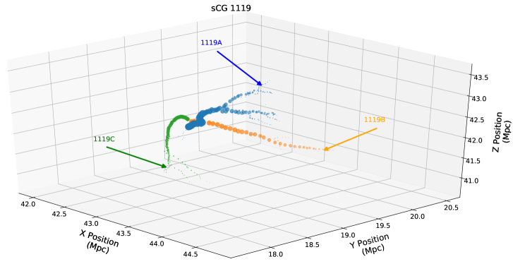
Figure 4: Same as Figure 2, but now showing sCG 1119. The final configuration of the group at $z=0$ is roughly at the center left of the figure as viewed in perspective. Galaxies are labeled A to C in order of decreasing $M_{\ast}$ at $z=0$.

In a handful of cases some snapshots had missing data in mGuo2010a. In such cases we linearly interpolated between the values in the two adjacent snapshots. The cause of the missing data is not entirely clear, but this seems to occur when galaxies come very close to one another, sometimes resulting in the least massive one not being detected in a snapshot. We only performed this interpolation where one of the main galaxies detected at $z=0$ was missing data at earlier times and only up to its last merging event. Our goal of tracing $z=0$ galaxies all the way back to the beginning of cosmic time inevitably means that, due to merging events, one or more of these will have split up into more than one galaxy at earlier times. In turn, one of the lower-mass precursor galaxies may be missing data; we do not interpolate such cases. The effect of this is minimal on the traced quantities, but it does explain why in a few cases some quantities, usually for the most massive galaxy A, show abrupt dips, e.g. in sCG 1056A at around 7.0 and 5.5 Gyr ago in $M_{\ast}$ and $M_{\rm CGas}$ (see Figure 7).

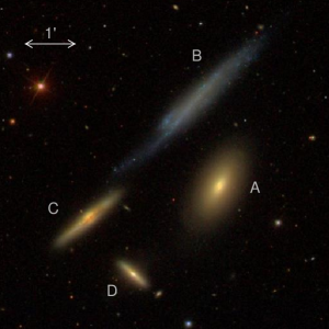
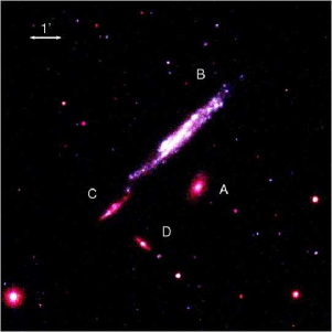
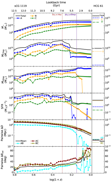
Figure 5: Top Left: SDSS optical image as in Figure 3, but now showing HCG 61. Bottom Left: Swift/UVOT color image as in Figure 3, also for HCG 61. Galaxy B is a foreground object. Right: Same as Figure 3, but instead showing sCG 1119 vs HCG 61. The color-coding for each sCG 1119 galaxy corresponds directly to that in the 3D merger tree shown in Figure 4. In order of decreasing stellar mass, sCG 1119B is best matched to HCG 61C, and sCG 1119C to HCG 61D.

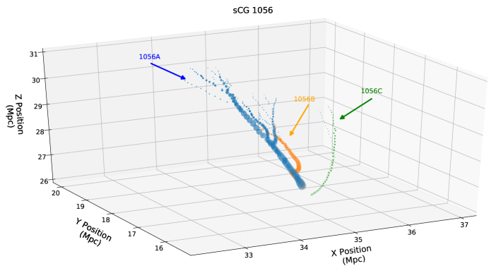
Figure 6: Same as Figure 2, but now showing sCG 1056. The final configuration of the group at $z=0$ is roughly at the lower center right of the figure as viewed in perspective. Galaxies are labeled A to C in order of decreasing $M_{\ast}$ at $z=0$.

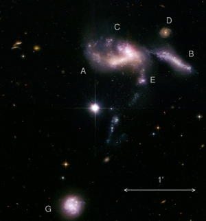
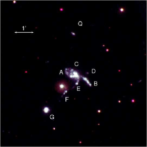
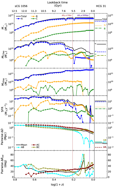
Figure 7: Top Left: Composite image of HCG 31 combining HST ACS ($B_{435}$, $V_{606}$, and $I_{814}$), HST WFPC2 ($B_{439}$, $V_{555}$, and $I_{814}$), GALEX (NUV), and Spitzer (8$\upmu$m NIR). Image credit: NASA, ESA, S. Gallagher and J. English(http://www.spacetelescope.org/images/opo1008a/). Bottom Left: Swift/UVOT color image as in Figure 3, but now showing HCG 31. Galaxy D is a background object, Q is likely physically associated but is quite small compared to the other associated galaxies (Rubin et al., 1990), and F is a tidal feature (Gallagher et al., 2010). Galaxies A and C appear to be undergoing an ongoing merger, and E is likely a tidal feature (López-Sánchez et al., 2004)(Galaxy E may be a tidal remnant and not a distinct galaxy.). Right: Same as Figure 3, but instead showing sCG 1056 vs HCG 31. The color-coding for each sCG 1056 galaxy corresponds directly to that in the 3D merger tree shown in Figure 6. In order of decreasing stellar mass, sCG 1056A is best matched to HCG 31ACE, sCG 1056B to HCG 31G, and sCG 1056C to HCG 31B. In the pairwise galaxy separation and velocity vector angle panels of HCG 31, we use the location of galaxy A to define the center of ACE.

cccMccMMMMM[ht] 0pt Observational HCG Sample      Group ID                 Coordinates (J2000)         $D_{\rm L}$a       $M_{*}$b       $M_{{\rm H}{\textsc{i}}}$c       $M_{\rm H_{2}}$d       $M_{\rm CGas}$e       $M_{\rm HGas}$f         SFRb    

     

$\alpha$ $\delta$ (Mpc) $\log(M_{\odot})$ $\log(M_{\odot}$ ${\rm yr}^{-1})$
(1) (2) (3) (4) (5) (6) (7) (8) (9) (10) (11) HCG 16 Group 02^h09^m31.3^s -10^∘0931 51.3 11.41 ¿10.44 10.52 ¿10.78 8.59+8.35 -8.30 1.52
A 02^h09^m24.6^s -10^∘0809 10.98 9.09 10.14 10.18 7.77+7.52 -7.52 0.62
B 02^h09^m20.8^s -10^∘0759 10.77 8.92 9.27 9.43 7.75+7.75 -7.22 -0.40
C 02^h09^m38.5^s -10^∘0848 10.79 9.50 9.87 10.02 8.37+8.09 -8.13 1.11
D 02^h09^m42.9^s -10^∘1103 10.54 ¿9.67 9.99 ¿10.16 7.58+7.14 -7.14 1.19
HCG 22 Group 03^h03^m31.3^s -15^∘4032 34.8 10.99 9.15 … ¿9.15 † … -0.08
A 03^h03^m38.4^s -15^∘3648 10.92 … ¡8.82 ¡8.82 ‡ … -0.56
B 03^h03^m26.1^s -15^∘3943 9.84 … … … … -1.30
C 03^h03^m24.5^s -15^∘3724 9.86 … ¡8.70 ¡8.70 ‡ … -0.30
HCG 31 Group 05^h01^m38.3^s -04^∘1525 55.7 10.49 10.37 ¡9.28 ¡10.40 … 1.07
ACEg 05^h01^m38.7^s -04^∘1534 10.32 9.67h ¡8.84h ¡9.73 … 0.96
B 05^h01^m36.2^s -04^∘1543 9.52 9.30 ¡8.80 ¡9.42 … -0.01
G 05^h01^m44.0^s -04^∘1720 9.81 9.30 ¡8.75 ¡9.41 … 0.22
HCG 37 Group 09^h13^m35.6^s +30^∘0051 96.8 11.17 9.21 ¡9.89i ¡9.97 … 0.26
A 09^h13^m39.4^s +29^∘5935 11.40 … 8.43i ¿8.43 ‡ … -0.20
B 09^h13^m33.1^s +30^∘0001 10.99 … 9.82i ¿9.82 ‡ … 0.04
C 09^h13^m37.3^s +29^∘5958 10.40 … ¡8.33i ¡8.33 ‡ … -0.95
D 09^h13^m33.8^s +30^∘0057 10.08 … 8.29i ¿8.29 ‡ … -0.37
E 09^h13^m34.0^s +30^∘0223 10.04 … 8.85i ¿8.85 ‡ … -0.70
HCG 48 Group 10^h37^m45.6^s -27^∘0450 43.7 11.16 8.54 … ¿8.54 † … 0.06
A 10^h37^m47.4^s -27^∘0454 11.03 … … … … -0.70
B 10^h37^m49.5^s -27^∘0718 10.29 … ¡8.35 ¡8.35 ‡ … -0.04
C 10^h37^m40.5^s -27^∘0329 10.11 … … … … -1.66
D 10^h37^m41.4^s -27^∘0240 9.68 … … … … -1.78
HCG 61 Group 12^h12^m24.9^s +29^∘1121 58.0 11.30 9.98 … ¿9.98 † … 0.69
A 12^h12^m18.8^s +29^∘1046 11.03 … 8.42 ¿8.42 ‡ … -0.22
C 12^h12^m31.0^s +29^∘1006 10.82 … 9.69 ¿9.69 ‡ … 0.61
D 12^h12^m26.9^s +29^∘0857 10.43 … … … … -0.67
Notes. Member galaxy properties for HCGs used in case studies. Column (1): CG name. Column (2): member galaxy ID. Column (3): R.A. Column (4): decl. Column (5): luminosity distance from NED^a. Column (6): stellar mass. Column (7): H i mass. Column (8): H₂ mass. Column (9): hot gas mass. Column (10): cold gas mass. Column (11): star formation rate. Group total values are sums of individual galaxy values, except where noted. ^a https://ned.ipac.caltech.edu/ ^b Lenkić et al. (2016). ^c Verdes-Montenegro et al. (2001). Much of the total group H i mass is not confined to individual galaxies and is thus not the sum of individual galaxy values. ^d Lisenfeld et al. (2017), except where noted. ^e $M_{\rm CGas}$ calculated as the sum of H i and H₂ gas masses, where available. The $\dagger$ indicates cases where only $M_{\rm H{\textsc{i}}}$ data were available, while the $\ddagger$ indicates the same for $M_{\rm H_{2}}$. In cases where the only available data are an upper limit for $M_{\rm H_{2}}$, this is indicated by $<$ and a $\ddagger$ in the $M_{\rm CGas}$ Column (9). ^f O’Sullivan et al. (2014). ^g Galaxies A, C, and E treated as a single entity by references. ^h Data for AC only. ⁱ $M_{\rm H_{2}}$ values for HCG 37 from  Martinez-Badenes et al. (2012).

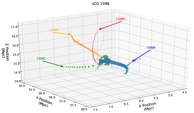
Figure 8: Same as Figure 2, but now showing sCG 1598. The final configuration of the group at $z=0$ is roughly at the center of the figure as viewed in perspective. Galaxies are labeled A to D in order of decreasing $M_{\ast}$ at $z=0$.

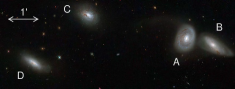
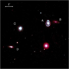
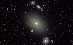
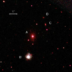
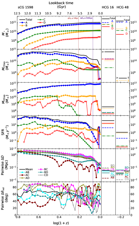
Figure 9: Top left: Composite image of HCG 16 combining HST WFPC2 ($B_{450}$, $V_{606}$, and $I_{814}$) and ESO Multi-Mode Instrument data. Image credit: NASA, ESA, ESO, and J. Charlton (http://www.spacetelescope.org/news/heic1514/). Second from top left: Swift/UVOT color image as in Figure 3, but now showing HCG 16. Second from bottom left: Dark Energy camera six filter ($U_{350}$, $G_{475}$, $R_{635}$, $I_{775}$, $Z_{925}$, and $Y_{1000}$) optical image of HCG 48. Image credit: Dane Kleiner (https://www.noao.edu/news/2014/pr1408-images.php). Bottom left: Swift/UVOT color image as in Figure 3, but now showing HCG 48. Right: Same as Figure 3, but instead showing sCG 1598 vs HCGs 16 and 48. The color-coding for each sCG 1598 galaxy corresponds directly to that in the 3D merger tree shown in Figure 8. The two right-most panels show values for the same quantities as in the left hand panels but for HCG 16 and HCG 48 as labeled (Table 7). In the case of HCG 16, galaxies B and C are not in order of decreasing stellar mass; the line color/style still reflects decreasing stellar mass, so sCG 1598B is now matched with HCG 16C, and sCG 1598C with HCG 16B.

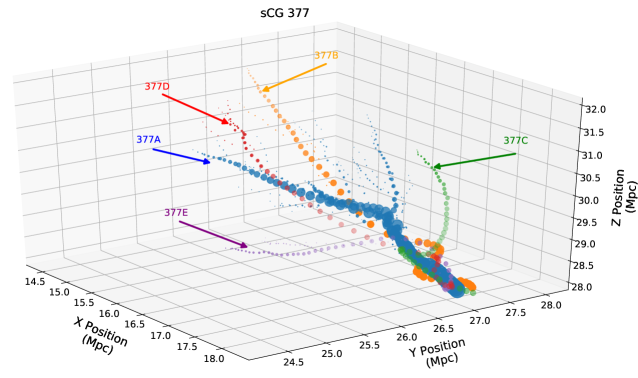
Figure 10: Same as Figure 2, but now showing sCG 377. The final configuration of the group at $z=0$ is roughly in the lower right of the figure as viewed in perspective. Galaxies are labeled A to E in order of decreasing $M_{\ast}$ at $z=0$.

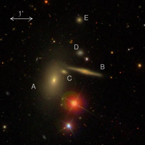
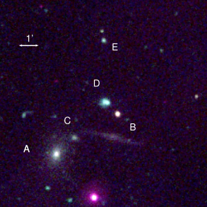
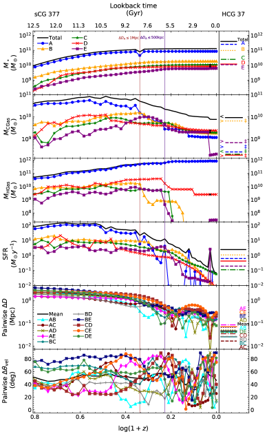
Figure 11: Top Left: SDSS optical image as in Figure 3, but now showing HCG 37. Bottom Left: Swift/UVOT color image as in Figure 3, also instead showing HCG 37. Right: Same as Figure 3, but instead showing sCG 377 vs HCG 37. The color-coding for each sCG 377 galaxy corresponds directly to that in the 3D merger tree shown in Figure 10. In the bottom two panels, the HCG 37 pairwise separations use the same naming and color- and symbol coding as in the corresponding sCG 377 panels.

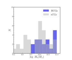
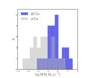
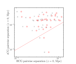
Figure 12: Distributions of $M_{\ast}$ (left) and SFR (middle) values for HCG (blue hatched) and sCG (gray) galaxies. The right panel shows sCG pairwise separations at $z=0$ against HCG pairwise separations for corresponding, $M_{\ast}$-ranked galaxies. The gray crosses are original projected separations, while red circles mark these separations multiplied by an empirically determined factor of $2\pi/5$ to “correct” them to reasonable deprojected separations. The red dashed line indicates equality.

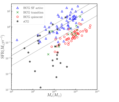
Figure 13: SFR vs. $M_{\ast}$ plot for CG galaxies in this paper, adapted from Lenkić et al. (2016). We used classification information from Zucker et al. (2016) to color-code HCGs according to their level of star-formation activity: blue triangles are actively star-forming, green crosses are transitioning, and red circles indicate quiescent galaxies. Black stars represent sCG galaxies from our study. The black line is the “star-forming main sequence” fit of Chang et al. (2015). The dotted lines indicate $\pm 1\sigma$ limits.

2.4 Results

We first describe results for the three different types of galaxy masses ($M_{\ast}$, $M_{\rm CGas}$, and $M_{\rm HGas}$, all at $z=0$) shown in Table 1, which show some clear and interesting patterns.

Among three-member systems, most show similar stellar-mass ranges at $z=0$: the stellar mass for their most massive galaxy is in the range $10^{10}\lesssim M_{\ast}/M_{\odot}\lesssim 10^{11}$. In comparison, the stellar mass of the second most massive galaxy is smaller by less than an order of magnitude. That said, member galaxies in sCG 518, sCG 1773, and sCG 2143 have $M_{\ast}$ values up to $\sim$1 order of magnitude smaller.

Regardless of the number of members, in all systems the cold gas mass shows a variable range, but its total value never exceeds $10^{10}$ $M_{\odot}$, which is well below the total stellar mass. The only exception is sCG 518, where $M_{\rm CGas}$ $=1.8$ $M_{\ast}$. In terms of $M_{\rm CGas}$ in individual galaxies and in triplets, in half of triplet sCGs the two galaxies that are least massive in $M_{\ast}$ (i.e., B and C) are more massive in $M_{\rm CGas}$ compared to galaxy A. The exceptions are sCG 1441 C, sCG 1757 B, and both B and C in sCG 518, sCG 1773, and sCG 2143. In contrast, with the exception of sCG 518, the total hot gas mass is consistently larger by up to about an order of magnitude than the total stellar mass. This is driven by the hot gas mass associated with the galaxy that has the highest $M_{\ast}$ (i.e., A). In most three-member sCGs galaxy A is also the galaxy with the highest $M_{\rm HGas}$, the exceptions being sCG 518 and sCG 1441.

In the single four-member sCG 1598, $M_{\ast}$ ranges from $10^{9.4}$ to $10^{11}$ $M_{\odot}$, and galaxy A has the least cold gas and the most hot gas mass, completely dominating the total hot gas mass. The five-member sCG 377 is similar: $M_{\ast}$ ranges from $10^{9.8}$ to $10^{11.12}$ $M_{\odot}$, and galaxy A is the second least massive galaxy in $M_{\rm CGas}$ while it provides the dominant contribution by more than three orders of magnitude to the group’s total hot gas mass.

Regarding the SFR values at $z=0$, overall these show relatively low values even if we exclude galaxies to which the Guo2010a semianalytical model assigns SFR values of zero. Comparing Columns (6) and (11) in Table 1, we see that, overall, SFRs for sCG galaxies were higher in the past, as expected. The only exception is sCG 1757, for which the mean SFR for $z\lesssim 0.28$ is almost an order of magnitude lower than at $z=0$. This is due to a spike in SFR at $z\sim 0$ for most massive galaxy A that dominates the SFR at $z=0$, and is due to a merger. Otherwise, a trend with SFR increasing with redshift also holds for this sCG. For the five sCGs that are most similar to HCGs in terms of $M_{\ast}$, it can be seen from the evolutionary plots that the most massive galaxies had SFRs about 100 times higher close to the beginning of cosmic time. Nevertheless, the general trend of decreasing SFRs is often interrupted by abrupt increases lasting several hundred Myr.

As can be seen in the evolutionary plots, there is considerable variety in the evolution of galaxy separations in the identified sCG sample. As mentioned already, once individual galaxies come within 1 or 0.5 Mpc of the most massive galaxy A, they stay within this distance to A until $z=0$. Considering separations between all pairs of galaxies, in sCG 115, sCG 377, sCG 1441, and sCG 1598, although at some point galaxies come as close as $\sim$100 kpc or less to each other, they then increase their separations up to $\sim$400 kpc. On the other hand, galaxies in other sCGs do not show this behavior and continuously come closer to each other. A comparison of the lower two left hand panels in the evolutionary plots shows that the degree of increase in $\Delta D$ after close approaches strongly correlates with the relative direction from which the group member galaxies are coming together. Thus, groups where the galaxies are coming together on fairly parallel paths (low $\Delta\theta_{\rm vel}$ values) do not experience large spikes in pairwise separation after close approaches, while groups whose member galaxies are coming from very different directions (high $\Delta\theta_{\rm vel}$) tend to experience more pronounced and abrupt changes in galaxy separations.

We highlight some specific cases for $\Delta D$ and $\Delta\theta_{\rm vel}$ evolution of particular interest. In sCG 377, which is the only five-member group (Figs 10 and 11), galaxy B has a closest approach of galaxy A at 57 kpc at $z=0.51$. It then recedes as far as 394 kpc from A at $z=0.28$. The closest the galaxies get to each other after this is at $z=0.04$ when they are 83 kpc from each other. This is in contrast to the general observation that, overall, sCG galaxies stay within 250 kpc after a first close encounter. In contrast, sCG 1056 A and sCG 1056 B come within 100 kpc at $z=0.28$ and remain within this separation until $z=0$, with several close approaches between 12 and 30 kpc. This suggests that these galaxies may be about to merge into a single system. On the other hand, sCG 1056 C remains more than 300 kpc away, although steadily approaching the other two members. In sCG 1119, galaxies A and B appear to be undergoing an ongoing merging process, with separations within 10 kpc in the past 540 Myr. Their first closest approach at 26 kpc is at $z=0.32$, and their maximum separation after this is 44 kpc with several closer approaches until $z=0$. Similarly, galaxies A and C in sCG 1773 have been within 30 kpc of each other for the past 3.5 Gyr (since $z=0.76$) with multiple close encounters within $\lesssim 10$ kpc. At the same time, sCG 1773 B is separated by at most 34 kpc from A or C during the past 1.1 Gyr, with a couple of close approaches between 3 and 14 kpc. In fact, this is the only sCG where by $z=0.24$ and all the way to $z=0$ all galaxies are within 100 kpc of each other with several close approaches. This system is thus a clear candidate for merging into a single galaxy. Alternatively, this sCG could turn into a so-called “fossil group”. Such groups have also been identified in the Millennium Simulation (Farhang et al., 2017). Fossil groups (Ponman et al. 1994; see also Dariush et al. 2010; Aguerri et al. 2011; Farhang et al. 2017; Kundert et al. 2017 and references therein) are characterized by an extended X-ray halo and are dominated by a large early-type galaxy, with a significantly fainter second-ranked galaxy (at least e mag fainter in $r$ within $R_{200}$, the radius of the sphere centered on the halo in which the critical density is 200 times the mean density of the universe; Jones et al., 2003). sCG 1773 could become a fossil group if at some point the second most massive (and presumably second-brightest) galaxy B merges with the most massive (and brightest) galaxy A, thus creating a large magnitude gap between the least massive (and least bright) galaxy C and the newly merged galaxy A+B.

In terms of angular separation evolution, the mean angular separation for the triplet sCG 115 is $\sim 40$ until $\sim 6$ Gyr ago. It then fluctuates by up to $\sim 60\%$ until $z=0$. For sCG 1119 the mean $\Delta\theta_{\rm vel}$ value is $\sim 20$ in early times, slowly increasing until $\sim 4$ Gyr ago, after which it increases significantly more rapidly until $z=0$. In sCG 1056 the mean angular separation is initially $\sim 40$, decreasing down to $\sim 20$ by $\sim 11$ Gyr ago. It remains at similarly small values until $z=0$ with a pronounced spike $\sim 2.9$ Gyr ago. For sCG 1598 the mean of $\sim 60$ is fairly stable until $\sim 2$ Gyr ago, but there are $\sim 30\%$ fluctuations for individual galaxies. sCG 377 shows similar behavior with a mean of $\sim 50$. There is thus noticeably different behavior in the cosmic evolution of the velocity vector angles between three-member and four- or five-member sCGs: While triplets show, on average, angles between 20 and 40, the two sCGs with more members show larger angles. In addition, $\Delta\theta_{\rm vel}$ fluctuations for individual galaxies are clearly more pronounced for the nontriplets. This suggests that, overall, the paths of triplets are, in comparison, much more undisturbed and closer to being parallel to each other. We postulate that the relative alignment of the galaxy velocity vectors allows these systems to be relatively long-lived. Furthermore, these long-lived triplets may be moving along narrow filaments, thus ensuring that they are likely to remain isolated.

3 Comparisons with Observed Compact Groups

To compare properties between our detected sCGs and CGs in the Hickson catalog (Hickson, 1982; Hickson et al., 1992), we used SFR and $M_{\ast}$ values from Lenkić et al. (2016), $M_{\rm H{\textsc{i}}}$ from Verdes-Montenegro et al. (2001), $M_{\rm H_{2}}$ from Lisenfeld et al. (2017) and Martinez-Badenes et al. (2012), and $M_{\rm HGas}$ values from O’Sullivan et al. (2014). We plot sCG and corresponding HCG properties as a function of redshift and cosmic time side by side in the evolutionary Figures 3, 5, 7, 9, and 11. Specifically, we plot all key quantities for sCG 115, sCG 1119, sCG 1056, sCG 1598, and sCG 377, together with corresponding values for HCG 22, HCG 61, HCG 31, HCG 16, and HCG 48 and HCG 37, respectively. In addition, in Figure 12 we show $M_{\ast}$ and SFR distributions, and we also plot pairwise velocity separations for HCG and sCG galaxies corresponding in stellar mass. For reference, we also provide a list of observational data and key properties for these six HCGs in Table 7, for both individual galaxies and entire groups. We first present an overview of these comparisons and then discuss individual sCG-HCG pairs.

Overall, we found that stellar mass is the property for which the greatest number (six) of well-known observed HCGs show reasonable to good agreement with at least one of the five sCGs plotted in the evolutionary figures. The agreement is within factors of a few for at least one member galaxy. This includes both the four- and five-member sCGs, as well as sCG 1056, which bears some particularly interesting similarities to HCG 31, a well-known and unusual system (e.g., Gallagher et al., 2010). However, although sCG stellar masses cover the full range of HCG values (Figure 12), we note that in 13 out of 17 (76%) of the HCG galaxies in the six groups compared, $M_{\ast}$ is higher by up to $\sim 0.9$ in the log (with a mean of $\sim 0.5$) compared to the corresponding $M_{\ast}$-ranked sCG galaxy.

Further, HCGs have systematically higher SFRs at $z=0$. This is the case not only in terms of total (group) rates but also usually when comparing corresponding $M_{\ast}$-ranked galaxies. It is also true regardless of whether an HCG is known to be more evolved (e.g., HCG 22) because of low SFRs, large amounts of diffuse X-ray gas, group H i content, or high fraction of ellipticals. A complementary way of comparing SFRs and stellar masses for sCGs and HCGs is to view them in the SFR vs. $M_{\ast}$ plane, shown in Figure 13. In this parameter space recent work has established a roughly linear correlation between log(SFR) and log($M_{\ast}$) known as the “star forming main sequence” (SFMS; Speagle et al., 2014, and references therein), and shown within $\pm 1\sigma$ by the straight lines in the figure. The correlation holds in both the local and the high-redshift universe (with an offset in normalization) and has also been extracted from cosmological simulations (e.g., Sparre et al., 2015). HCG galaxies as a whole appear to follow the correlation, although they show considerable scatter and nonactively star forming HCGs fall systematically below it. It is striking that our identified sCGs as a whole do not follow the correlation. In particular, there are no sCG galaxies with $M_{\ast}$ $\gtrsim 10^{11}$ $M_{\odot}$, while there is a tail of low-SFR, low-$M_{\ast}$ galaxies below the correlation.

On the other hand, separations between pairs of member galaxies are systematically smaller for HCGs. This is so even when we correct for the fact that we can only measure projected separations for HCGs. We carried out Monte Carlo simulations randomly positioning galaxies in 3D space and then measured both 2D and 3D separations. We deduced that the median 3D distance is a factor of $2\pi/5$ greater than the median projected distance. In the right panel of Figure 12 we plot sCG pairwise separations against both projected and corrected HCG pairwise separations, showing that sCGs have systematically larger separations by up to more than an order of magnitude in the most extreme cases.

3.1 $M_{\ast}$ and SFR Comparisons for Individual sCG–HCG Systems

We now briefly compare corresponding properties of specific sCG and HCG systems, chosen because they are overall closest in $M_{\ast}$. We compare corresponding $M_{\ast}$-ranked galaxies. Note that although for sCGs this ranking is always in alphabetical order, with A the most massive galaxy, for HCGs this is not always so for historical reasons: Hickson (1982) labeled CG galaxies by letter in order of decreasing $B$-band brightness. Specifically, HCG 22C is more massive than HCG 22B, HCG 31G is more massive than HCG 31B, and HCG 16C is more massive than HCG 16B.

3.1.1 sCG 115–HCG 22

The stellar masses of corresponding $M_{\ast}$-ranked galaxies show very close agreement, within factors of up to $\sim 3$ for this pair of triplets. SFRs for HCG 22 galaxies are larger than for sCG 115 ones at $z=0$ by more than an order of magnitude, but comparable to the values $2-3$ Gyr ago.

3.1.2 sCG 1119–HCG 61

The stellar masses for HCG 61 galaxies are all about half an order of magnitude higher than those of the corresponding galaxies of sCG 1119. Compared to corresponding sCG galaxies, the SFR is more than two orders of magnitude higher for HCG A and B, but less than an order of magnitude lower for HCG C.

3.1.3 sCG 1056–HCG 31

Although HCG 31 nominally consists of four galaxies, galaxies A and C are in an advanced merging stage forming essentially one morphologically peculiar system. “Galaxy” E is likely a tidal feature that overlaps closely with A and C, and so all of the A–C–E complex is often treated as a single entity for measuring quantities such as $M_{\ast}$ or SFR. In a somewhat similar fashion, sCG 1056 consists of only three galaxies, but, as can be seen from its merger tree (Figure 6), its galaxy A consisted of three galaxies in the past. This three-galaxy system first appears at $z\sim 0.62\ (\sim 5.7$ Gyr ago). Two subsequent mergers transform it first into a two-galaxy system at $z\sim 0.32\ (\sim 3.5$ Gyr ago) and finally into a single galaxy at $z\sim 0.06\ (\sim 0.83$ Gyr ago).

3.1.4 sCG 1598–HCGs 16 and HCG 48

These are all four-galaxy systems. HCG 16A agrees in $M_{\ast}$ with sCG 1598A within a factor of $\sim$2; however all other HCG galaxy $M_{\ast}$ values are higher than for their corresponding sCG galaxies by an order of magnitude or more. The situation for SFRs is similar. In contrast, HCG 48 shows the best agreement (within a factor of less than $\sim 2$) in stellar masses between the single four-member sCG and any known four-member HCG. In addition, two of the HCG 48 SFR values are also within factors of a few from their corresponding sCG ones; the exceptions are HCG 48A and HCG 48C.

3.1.5 sCG 377–HCG 37

Although $M_{\ast}$ values are overall higher for HCG galaxies, this pair represents the closest agreement (factors of a few to less than an order of magnitude in $M_{\ast}$) between the single sCG with five galaxies and a five-member HCG. Apart from galaxy C, HCG SFRs at $z=0$ are more than an order of magnitude higher than those of sCG galaxies. Instead, they are comparable to sCG SFRs $\sim 5$ Gyr ago.

4 Discussion

The milli-Millennium Simulation is a chunk of the full Millennium Simulation with 512 times smaller volume. As a result, the identified sCGs, their cosmological evolution, and their comparisons with HCGs represent interesting but essentially random case studies of CG-like systems identified at $z=0$ in a small part of the galaxy catalog produced by applying the semianalytical model of Guo et al. (2011) to the full Millennium Simulation. We are unable, and do not attempt, to draw any statistically robust conclusions regarding the frequency of occurrence of CGs, whether similar or not to observed systems; this is well beyond the scope of this analysis. That said, the variety of cosmological evolutionary paths identified suggests that there are several ways of leading to observed systems collectively known as CGs. In spite of differences from observed HCGs, it is clear from their merger tree evolution that in sCGs galaxies interact and influence each other, and eventually become bound. The essence of what we understand as a CG is thus an inherent characteristic of these systems.

Compared to HCGs, sCGs are selected differently, the essential initial criterion being proximity within a 3D volume (Section 2.2) with isolation applied subsequently. In contrast, the initial selection of HCGs used surface brightness and isolation criteria on galaxy groupings projected on the sky. In addition, the simulation volume is limited, and even more so for the particular catalog used. Even so, we can attempt to formally estimate how many “HCG-like” systems one might expect to detect as follows. The median redshift of the 92 HCGs with “accordant” galaxy velocities (spectroscopically verified to be within $\pm 1000$ km s^-1 of the group median) is $z=0.03$. Using this redshift value, over 67% of the sky Hickson et al. (1992) detected 47 CGs with accordant velocities. The true number of CGs over 67% of the sky to this redshift is then $N_{\rm HCG}=47/f$, where $f$ is a completeness factor equal to unity in the ideal case of a catalog with no incompleteness. Further, the luminosity distance and comoving volume to this redshift are $D_{L}=92.1\,h^{-1}$ Mpc and $V=(\Delta\Omega/3)(D_{L}/(1+z))^{3}$, respectively, where $\Delta\Omega=8\pi/3$ is the solid angle subtended by 67% of the sky. The expected number density of HCGs to $z=0.03$ is then $n_{\rm HCG}=2.3\times 10^{-5}\,h^{3}\,f^{-1}{\rm Mpc}^{-3}$. The volume of a snapshot of the milli-Millennium Simulation is $V_{\rm snap}=(62.5~{}h^{-1}{\rm Mpc})^{3}=2.44\times 10^{5}\,h^{-3}$ Mpc³, and there is one snapshot at $z=0$. Within this volume, one would expect to find $N_{\rm sim}\sim 6f^{-1}$ HCGs at $z=0$. If the sCG volume density were the same as the true volume density of HCGs, our detection of 10 systems might suggest a completeness factor of $\sim 55\%$ for HCGs. However, the differences in selection criteria between 3D space sCGs and HCGs projected on the sky are significant. In addition, the completeness factor estimated from simulations can be as low as 8% (Díaz-Giménez & Mamon, 2010), depending on the method and semianalytic model used (see Knebe et al. 2015, 2018 for a thorough discussion of the effects of different semianalytic models; see also Snaith et al. 2011).

Overall, the property that shows the best agreement between HCGs and sCGs is stellar mass. This is consistent with the fact that the Guo et al. (2011) semianalytical model uses the observed stellar mass function of galaxies as a primary constraint on several parameters related to star formation and feedback (their Table 1). However, when we compare the simulated versus observed CGs in greater detail, we see that, unlike known HCGs, we do not detect sCG galaxies with $M_{\ast}$ $\gtrsim 10^{11}$ $M_{\odot}$. In contrast, we detect several low to extremely low SFR and $M_{\ast}$ sCG galaxies (Figures 12 and 13). A lack of high-$M_{\ast}$ galaxies is perhaps not surprising, given the small simulation volume, as such galaxies are rarer. Note that detection of these galaxies is a direct result of semianalytical rather than full hydrodynamic modeling, so buildup of mass related to intragroup gas, which is known to play a significant role in CGs, may not be properly taken into account. On the other hand, detection of more low-$M_{\ast}$ systems is consistent with the fact that the Guo et al. (2011) model somewhat overpredicts the abundance of galaxies in the $M_{\ast}$ range of our detected sCGs (their Fig. 7), and even more so for low SFRs. The systematically lower SFRs for mGuo2010a groups (sCGs) compared to observations are consistent with a more general trend for lower SFRs in Guo et al. (2011) (their Fig. 22 and associated discussion). In addition, our selection is done in 3D space, which is not fully equivalent to the selection of HCGs in projection. Furthermore, it is observationally much harder to detect extremely low SFR systems (which would be fainter in the optical images used for selection by Hickson 1982 than more actively star-forming systems); relatively few studies targeting dwarf galaxy populations have been carried out for individual CGs, yielding few, mostly spectroscopically unconfirmed results (e.g. Ribeiro et al. 1994; Krusch et al. 2006; Konstantopoulos et al. 2012, 2013; Ordenes-Briceño et al. 2016; Shi et al. 2017, but see Zabludoff & Mulchaey 1998; Carrasco et al. 2006; Da Rocha et al. 2011). This may explain the low-SFR tail obtained for sCGs, combined with the dearth of massive galaxies. No strong conclusion can be made in any case, as we do not have a complete simulation sample in any statistical sense. That said, qualitatively we do observe similar behavior in $M_{\ast}$ vs. SFR space, where for the same sCG one or more galaxies may be within 1$\sigma$ of the observed correlation, while one or more may lie below.

We note that our clues selection is based on separation and isolation criteria in 3D. Thus, in a sense sCGs are guaranteed to represent physically compact and isolated systems, perhaps more so than observed HCGs. With no constraints on relative velocity, however, they are not guaranteed to be bound. Nonetheless, the fact that velocity vectors stay largely aligned and the systems are isolated suggests that they are expected to be long-lived, unlike, for example, Stephan’s Quintet (HCG 92). HCG 92 has a galaxy, NGC 7318B, that is likely only transiently interacting with the rest of the HCG 92 member galaxies. Taken at face value, the long lifetimes of the $z=0$ sCGs (see Columns (8) and (10) in Table 1) support the idea that at least some CGs are not transient concentrations. Such examples bring to mind the local example of HCG 7, a quartet of galaxies that appear to be relatively undisturbed morphologically, but whose properties such as H i mass and distribution and population of globular clusters indicate an extended period of group evolution without evidence for a major merger (Konstantopoulos et al., 2010).

Finally, although observed HCGs appear to be systematically more compact than sCGs, the discrepancy in pairwise galaxy separations will at least partially be affected by projection effects. For instance, sCG triplets evolve along roughly parallel paths in 3D. Depending on viewing angle, these can be projected on the sky to appear almost as compact as HCGs.

5 Summary and Conclusions

We used the clues algorithm to identify and characterize 10 CGs of galaxies in a portion of the semianalytical galaxy catalog of Guo et al. (2011), corresponding to the milli-Millennium cosmological simulation (sCGs in the mGuo2010a). We further compared key properties of these to those of observed HCGs. This work provides an independent cross-check of the Guo2010a semianalytical model by probing a regime that the model was not tuned to. Our main conclusions are as follows:

1. With sCG stellar masses in the range $10^{10}\lesssim M_{\ast}/M_{\odot}\lesssim 10^{11}$, $M_{\ast}$ is the property for which the greatest number (six) of HCGs have at least one galaxy that agrees within factors of a few with sCG galaxies at $z=0$. However, most (76%) HCG galaxies have higher $M_{\ast}$ than sCG ones.

2. Once sCG galaxies come within 1 (0.5) Mpc of their most massive galaxy, they remain within that distance until $z=0$. The typical redshifts for these “birthdays” indicate that $z=0$ sCGs are long-lived systems, with ages in the range of 5.7–11.4 Gyr (1.1–8.9 Gyr for the $\Delta D_{\rm A}=0.5$ Mpc criterion).

3. The pairwise separations of sCG galaxies show a variety of cosmological evolution. Although some exhibit a roughly oscillatory behavior, we identify one system where member galaxies consistently come closer to each other, a clear candidate for merging into a single galaxy or becoming a “fossil” group.

4. We define the angular pairwise 3D velocity vector separation, $\Delta\theta_{\rm vel}$, to capture the qualitative distinction between galaxies that approach on trajectories that can be characterized as “collision courses” (e.g., sCG 1598; Fig. 8) vs. galaxies on more parallel tracks (e.g., sCG 1056; Fig. 6). We speculate that the latter are expected to be more long-lived, with fewer instances of major mergers.

5. Triplet galaxies show the smallest changes in pairwise separations after close encounters and appear to travel across more parallel paths over cosmic times compared to nontriplets, thus making it more likely that they are not transient systems.

6. Only some sCG galaxies follow the SFR–$M_{\ast}$ correlation, with no galaxies with $M_{\ast}$ $\gtrsim 10^{11}$ $M_{\odot}$ and a tail of low SFR and $M_{\ast}$.

7. At $z=0$, HCG galaxies have systematically higher SFRs than sCG members by up to more than an order of magnitude.

8. With a few exceptions, pairwise galaxy separations are systematically smaller for HCGs; it is unclear how important projection effects are in this respect.

Given the small volume of the simulation and the handful of identified sCGs, no results of a statistical nature can be drawn. Our results are case studies of possible pathways to CGs at $z=0$. The probability of these particular pathways in the real universe remains unknown, while other pathways are likely possible. These results should be considered as a launching point for further, more detailed work, using larger and more recent simulations in tandem with observational catalogs.

References

- Aguerri et al. (2011) Aguerri, J. A. L., Girardi, M., Boschin, W., et al. 2011, A&A, 527, A143
- Alatalo et al. (2015) Alatalo, K., Appleton, P. N., Lisenfeld, U., et al. 2015, ApJ, 812, 117
- Amram et al. (2004) Amram, P., Mendes de Oliveira, C., Plana, H., et al. 2004, ApJ, 612, L5
- Astropy Collaboration et al. (2013) Astropy Collaboration, Robitaille, T. P., Tollerud, E. J., et al. 2013, A&A, 558, A33
- Barton et al. (1996) Barton, E., Geller, M., Ramella, M., Marzke, R. O., & da Costa, L. N. 1996, AJ, 112, 871
- Blaizot et al. (2005) Blaizot, J., Wadadekar, Y., Guiderdoni, B., et al. 2005, MNRAS, 360, 159
- Caliński & Harabasz (1974) Caliński, T., & Harabasz, J. 1974, Communications in Statistics. Theory and Methods, 3, 1
- Carrasco et al. (2006) Carrasco, E. R., Mendes de Oliveira, C., & Infante, L. 2006, AJ, 132, 1796
- Chang et al. (2010) Chang, F., Qiu, W., Zamar, R., Lazarus, R., & Wang, X. 2010, Journal of Statistical Software, 33, 1
- Chang et al. (2015) Chang, Y.-Y., van der Wel, A., da Cunha, E., & Rix, H.-W. 2015, ApJS, 219, 8
- Cluver et al. (2013) Cluver, M. E., Appleton, P. N., Ogle, P., et al. 2013, ApJ, 765, 93
- Coenda et al. (2012) Coenda, V., Muriel, H., & Martínez, H. J. 2012, A&A, 543, A119
- Coenda et al. (2015) —. 2015, A&A, 573, A96
- Da Rocha et al. (2011) Da Rocha, C., Mieske, S., Georgiev, I. Y., et al. 2011, A&A, 525, A86
- Dariush et al. (2010) Dariush, A. A., Raychaudhury, S., Ponman, T. J., et al. 2010, MNRAS, 405, 1873
- De Lucia & Blaizot (2007) De Lucia, G., & Blaizot, J. 2007, MNRAS, 375, 2
- Deng et al. (2007) Deng, X.-F., He, J.-Z., Jiang, P., et al. 2007, Astrophysics, 50, 18
- Díaz-Giménez & Mamon (2010) Díaz-Giménez, E., & Mamon, G. A. 2010, MNRAS, 409, 1227
- Díaz-Giménez et al. (2012) Díaz-Giménez, E., Mamon, G. A., Pacheco, M., Mendes de Oliveira, C., & Alonso, M. V. 2012, MNRAS, 426, 296
- Díaz-Giménez & Zandivarez (2015) Díaz-Giménez, E., & Zandivarez, A. 2015, A&A, 578, A61
- Farhang et al. (2017) Farhang, A., Khosroshahi, H. G., Mamon, G. A., Dariush, A. A., & Raouf, M. 2017, ApJ, 840, 58
- Freedman et al. (2012) Freedman, W. L., Madore, B. F., Scowcroft, V., et al. 2012, ApJ, 758, 24
- Gallagher et al. (2010) Gallagher, S. C., Durrell, P. R., Elmegreen, D. M., et al. 2010, AJ, 139, 545
- Guo et al. (2013) Guo, Q., White, S., Angulo, R. E., et al. 2013, MNRAS, 428, 1351
- Guo et al. (2010) Guo, Q., White, S., Li, C., & Boylan-Kolchin, M. 2010, MNRAS, 404, 1111
- Guo et al. (2011) Guo, Q., White, S., Boylan-Kolchin, M., et al. 2011, MNRAS, 413, 101
- Henriques et al. (2012) Henriques, B. M. B., White, S. D. M., Lemson, G., et al. 2012, MNRAS, 421, 2904
- Hickson (1982) Hickson, P. 1982, ApJ, 259, 930
- Hickson et al. (1992) Hickson, P., Mendes de Oliveira, C., Huchra, J. P., & Palumbo, G. G. 1992, ApJ, 399, 353
- Hinshaw et al. (2013) Hinshaw, G., Larson, D., Komatsu, E., et al. 2013, ApJS, 208, 19
- Johnson et al. (2007) Johnson, K. E., Hibbard, J. E., Gallagher, S. C., et al. 2007, AJ, 134, 1522
- Jones et al. (2003) Jones, L. R., Ponman, T. J., Horton, A., et al. 2003, MNRAS, 343, 627
- Karachentsev (2005) Karachentsev, I. D. 2005, AJ, 129, 178
- Knebe et al. (2015) Knebe, A., Pearce, F. R., Thomas, P. A., et al. 2015, MNRAS, 451, 4029
- Knebe et al. (2018) Knebe, A., Pearce, F. R., Gonzalez-Perez, V., et al. 2018, MNRAS, 475, 2936
- Konstantopoulos et al. (2010) Konstantopoulos, I. S., Gallagher, S. C., Fedotov, K., et al. 2010, ApJ, 723, 197
- Konstantopoulos et al. (2012) —. 2012, ApJ, 745, 30
- Konstantopoulos et al. (2013) Konstantopoulos, I. S., Maybhate, A., Charlton, J. C., et al. 2013, ApJ, 770, 114
- Krusch et al. (2006) Krusch, E., Rosenbaum, D., Dettmar, R.-J., et al. 2006, A&A, 459, 759
- Kundert et al. (2017) Kundert, A., D’Onghia, E., & Aguerri, J. A. L. 2017, ApJ, 845, 45
- Lee et al. (2004) Lee, B. C., Allam, S. S., Tucker, D. L., et al. 2004, AJ, 127, 1811
- Lee et al. (2014) Lee, J., Yi, S. K., Elahi, P. J., et al. 2014, MNRAS, 445, 4197
- Lenkić et al. (2016) Lenkić, L., Tzanavaris, P., Gallagher, S. C., et al. 2016, MNRAS, 459, 2948
- Lisenfeld et al. (2017) Lisenfeld, U., Alatalo, K., Zucker, C., et al. 2017, A&A, 607, A110
- López-Sánchez et al. (2004) López-Sánchez, Á. R., Esteban, C., & Rodríguez, M. 2004, ApJS, 153, 243
- Martínez et al. (2013) Martínez, H. J., Coenda, V., & Muriel, H. 2013, A&A, 557, A61
- Martinez-Badenes et al. (2012) Martinez-Badenes, V., Lisenfeld, U., Espada, D., et al. 2012, A&A, 540, A96
- McConnachie et al. (2008) McConnachie, A. W., Ellison, S. L., & Patton, D. R. 2008, MNRAS, 387, 1281
- McConnachie et al. (2009) McConnachie, A. W., Patton, D. R., Ellison, S. L., & Simard, L. 2009, MNRAS, 395, 255
- Mendes de Oliveira et al. (2003) Mendes de Oliveira, C., Amram, P., Plana, H., & Balkowski, C. 2003, AJ, 126, 2635
- Mendes de Oliveira et al. (2005) Mendes de Oliveira, C., Coelho, P., González, J. J., & Barbuy, B. 2005, AJ, 130, 55
- Mendes de Oliveira et al. (1998) Mendes de Oliveira, C., Plana, H., Amram, P., Bolte, M., & Boulesteix, J. 1998, ApJ, 507, 691
- Mineo et al. (2012) Mineo, S., Gilfanov, M., & Sunyaev, R. 2012, MNRAS, 419, 2095
- Mulchaey (2000) Mulchaey, J. S. 2000, ARA&A, 38, 289
- Ordenes-Briceño et al. (2016) Ordenes-Briceño, Y., Taylor, M. A., Puzia, T. H., et al. 2016, MNRAS, 463, 1284
- O’Sullivan et al. (2014) O’Sullivan, E., Zezas, A., Vrtilek, J. M., et al. 2014, ApJ, 793, 73
- Plana et al. (1998) Plana, H., Mendes de Oliveira, C., Amram, P., & Boulesteix, J. 1998, AJ, 116, 2123
- Ponman et al. (1994) Ponman, T. J., Allan, D. J., Jones, L. R., et al. 1994, Nature, 369, 462
- Proctor et al. (2004) Proctor, R. N., Forbes, D. A., Hau, G. K. T., et al. 2004, MNRAS, 349, 1381
- R Core Team (2012) R Core Team. 2012, R: A Language and Environment for Statistical Computing, R Foundation for Statistical Computing, Vienna, Austria. https://www.R-project.org
- Ribeiro et al. (1994) Ribeiro, A. L. B., de Carvalho, R. R., & Zepf, S. E. 1994, MNRAS, 267, L13
- Rose (1977) Rose, J. A. 1977, ApJ, 211, 311
- Rousseeuw (1987) Rousseeuw, P. J. 1987, Journal of Computational and Applied Mathematics, 20, 53
- Rubin et al. (1990) Rubin, V. C., Hunter, D. A., & Ford, Jr., W. K. 1990, ApJ, 365, 86
- Shi et al. (2017) Shi, D. D., Zheng, X. Z., Zhao, H. B., et al. 2017, ApJ, 846, 26
- Snaith et al. (2011) Snaith, O. N., Gibson, B. K., Brook, C. B., et al. 2011, MNRAS, 415, 2798
- Sparre et al. (2015) Sparre, M., Hayward, C. C., Springel, V., et al. 2015, MNRAS, 447, 3548
- Speagle et al. (2014) Speagle, J. S., Steinhardt, C. L., Capak, P. L., & Silverman, J. D. 2014, ApJS, 214, 15
- Springel et al. (2005) Springel, V., White, S. D. M., Jenkins, A., et al. 2005, Nature, 435, 629
- Torres-Flores et al. (2014) Torres-Flores, S., Amram, P., Mendes de Oliveira, C., et al. 2014, MNRAS, 442, 2188
- Torres-Flores et al. (2010) Torres-Flores, S., Mendes de Oliveira, C., Amram, P., et al. 2010, A&A, 521, A59
- Torres-Flores et al. (2009) Torres-Flores, S., Mendes de Oliveira, C., de Mello, D. F., et al. 2009, A&A, 507, 723
- Tzanavaris et al. (2016) Tzanavaris, P., Hornschemeier, A. E., Gallagher, S. C., et al. 2016, ApJ, 817, 95
- Tzanavaris et al. (2010) —. 2010, ApJ, 716, 556
- Verdes-Montenegro et al. (2001) Verdes-Montenegro, L., Yun, M. S., Williams, B. A., et al. 2001, A&A, 377, 812
- Walker et al. (2012) Walker, L. M., Johnson, K. E., Gallagher, S. C., et al. 2012, AJ, 143, 69
- Walker et al. (2010) —. 2010, AJ, 140, 1254
- Walker et al. (2013) Walker, L. M., Butterfield, N., Johnson, K., et al. 2013, ApJ, 775, 129
- Wang et al. (2007) Wang, X., Qiu, W., & Zamar, R. H. 2007, Comp. Stat. Data Anal., 52, 286
- Wetzel et al. (2012) Wetzel, A. R., Tinker, J. L., & Conroy, C. 2012, MNRAS, 424, 232
- Zabludoff & Mulchaey (1998) Zabludoff, A. I., & Mulchaey, J. S. 1998, ApJ, 496, 39
- Zucker et al. (2016) Zucker, C., Walker, L. M., Johnson, K., et al. 2016, ApJ, 821, 113