OGLE-2016-BLG-0156: Microlensing Event With Pronounced Microlens-Parallax Effects Yielding Precise Lens Mass Measurement

Abstract

We analyze the gravitational binary-lensing event OGLE-2016-BLG-0156, for which the lensing light curve displays pronounced deviations induced by microlens-parallax effects. The light curve exhibits 3 distinctive widely-separated peaks and we find that the multiple-peak feature provides a very tight constraint on the microlens-parallax effect, enabling us to precisely measure the microlens parallax $\pi_{\rm E}$. All the peaks are densely and continuously covered from high-cadence survey observations using globally located telescopes and the analysis of the peaks leads to the precise measurement of the angular Einstein radius $\theta_{\rm E}$. From the combination of the measured $\pi_{\rm E}$ and $\theta_{\rm E}$, we determine the physical parameters of the lens. It is found that the lens is a binary composed of two M dwarfs with masses $M_{1}=0.18\pm 0.01\ M_{\odot}$ and $M_{2}=0.16\pm 0.01\ M_{\odot}$ located at a distance $D_{\rm L}=1.35\pm 0.09\ {\rm kpc}$. According to the estimated lens mass and distance, the flux from the lens comprises an important fraction, $\sim 25\%$, of the blended flux. The bright nature of the lens combined with the high relative lens-source motion, $\mu=6.94\pm 0.50\ {\rm mas}\ {\rm yr}^{-1}$, suggests that the lens can be directly observed from future high-resolution follow-up observations.

1. Introduction

The microlensing phenomenon occurs by the gravity of lensing objects regardless of their luminosity. Due to this property, microlensing provides an important tool to detect very faint and even dark objects that cannot be observed by other methods. However, it is difficult to conclude the faint/dark nature of the lens just based on the event timescale $t_{\rm E}$, which is the only observable related to the lens mass for general lensing events, because the timescale is related to not only the lens mass $M$ but also the relative lens-source proper motion $\mu$ and distance to the lens $D_{\rm L}$ and source $D_{\rm S}$ by

$$t_{\rm E}={\theta_{\rm E}\over\mu};\qquad\theta_{\rm E}=\sqrt{\kappa M\pi_{\rm rel}};\qquad\pi_{\rm rel}={\rm au}\left({1\over D_{\rm L}}-{1\over D_{\rm S}}\right),$$ (1)

where $\kappa=4G/(c^{2}{\rm au})$ and $\theta_{\rm E}$ is the angular Einstein radius. In order to reveal the nature of lenses, their masses should be determined.

For the unique determination of the lens mass, it is required to measure two additional observables. These observables are the angular Einstein radius $\theta_{\rm E}$ and the microlens parallax $\pi_{\rm E}$. They are related to the lens mass by (Gould, 2000)

$$M={\theta_{\rm E}\over\kappa\pi_{\rm E}}.$$ (2)

With $\pi_{\rm E}$ and $\theta_{\rm E}$, the distance to the lens is also determined by

$$D_{\rm L}={{\rm au}\over\pi_{\rm E}\theta_{\rm E}+\pi_{\rm S}},$$ (3)

where $\pi_{\rm S}={\rm au}/D_{\rm S}$.

The angular Einstein radius is determined by detecting deviations in lensing light curves caused by finite-source effects. Deviations induced by finite-source effects arise due to the differential magnification in which different parts of the source surface are magnified by different amount. For events produced by single mass objects, finite-source effects can be detected in the special case in which the lens passes over the surface of the source (Witt & Mao, 1994; Gould, 1994a; Nemiroff & Wickramasinghe, 1994). However, the ratio of the angular source radius $\theta_{*}$ to the angular Einstein radius $\theta_{\rm E}$ is very small, $\rho~{}\sim 1/1000$ for events associated with main-sequence source stars and $\sim~{}1/100$ even for events involved with giant source stars, and thus the rate of source-crossing events is accordingly very low. The chance to detect finite-source effects is relatively much higher for events produced by binary objects. This is because a binary lens forms caustics that can extend over an important portion of the Einstein ring, and the event with a source crossing the caustic exhibits a light curve affected by the finite-source effect during the caustic crossing.

In the early-generation lensing surveys that were conducted with a $>1$ day cadence, measuring the angular Einstein radius by detecting finite-source effects was observationally a challenging task. This is because the duration of the deviation induced by finite-source effects is, in most cases, $<1$ day and thus it was difficult to detect the deviation. The unpredictable nature of caustic crossings also made it difficult to cover crossings from high-cadence follow-up observations (Jaroszyński & Mao, 2001). However, with the inauguration of lensing surveys using globally distributed multiple telescopes equipped with wide-field cameras, the observational cadence has been dramatically increased to $<1$ hour, making it possible to measure $\theta_{\rm E}$ for a greatly increased number of lensing events.

One channel to measure the microlens parallax is simultaneously observing lensing events from the ground and in space: ‘space-based microlens parallax’ (Refsdal, 1966; Gould, 1994b). The physical size of the Einstein radius for a typical lensing event is of the order of au. Then, if space observations are conducted using a satellite in a heliocentric orbit, e.g., Deep Impact (Muraki et al., 2011) spacecraft or Spitzer Space Telescope (Dong et al., 2007; Calchi Novati et al., 2015; Udalski et al., 2015b), the lensing light curve obtained from the satellite observation will be substantially different from that obtained from the ground-based observation. For events with well covered light curves from both the ground and in space, then, the microlens parallax can be precisely measured by comparing the two light curves.

Another channel to measure $\pi_{\rm E}$ is analyzing deviations induced by microlens-parallax effects in lensing light curves obtained from ground-based observations: ‘annual microlens parallax’ (Gould, 1992). In the single frame of Earth, such deviations occur due to the positional change of an observer caused by the orbital motion of Earth around the Sun. For typical lensing events produced by low-mass stars, however, the event timescale is several dozen days, which comprises a small fraction of the orbital period of Earth, i.e., year, and thus deviations induced by the annual microlens-parallax effects are usually very minor. As a result, it is difficult to detect the parallax-induced deviations for general events, and even for events with detected deviations, the uncertainties of the measured $\pi_{\rm E}$ and the resulting lens mass can be considerable.

In this work, we analyze the binary-lensing event OGLE-2016-BLG-0156. The light curve of the event, which is characterized by three distinctive widely-separated peaks, exhibits pronounced parallax-induced deviations, from which we precisely measure the microlens parallax. All the peaks are densely covered from continuous and high-cadence survey observations and the analysis of the peaks leads to the precise measurement of the angular Einstein radius. We characterize the lens by measuring the masses of the lens components from $\pi_{\rm E}$ and $\theta_{\rm E}$.

2. Observation and Data

The source star of the lensing event OGLE-2016-BLG-0156 is located in the bulge field with equatorial coordinates $({\rm R.A.},{\rm decl.})_{\rm J2000}=(17:56:36.63,-31:04:40.7)$. The corresponding galactic coordinates are $(l,b)=(359.4^{\circ},-3.14^{\circ})$. The event was found in the very early part of the 2016 bulge season by the Optical Gravitational Lensing Experiment (OGLE: Udalski et al., 2015a) survey. The OGLE lensing survey was conducted using the 1.3 m telescope of the Las Campanas Observatory, Chile. The source brightness had remained constant, with a baseline magnitude of $I_{\rm base}\sim 18.74$, until the end of the 2015 season since it was monitored by the survey in 2009. When the event was found, the source brightness was already $\sim 0.5$ magnitude brighter than the baseline magnitude, indicating that the event started during the $\sim 4$ month time gap between the 2015 and 2016 seasons when the bulge field could not be observed during the passage of the field behind the Sun. The OGLE observations were conducted at a $\sim 1$–2 day cadence and data were acquired mainly in $I$ band with some $V$ band data obtained for the source color measurement.

Two other microlensing survey groups of the Microlensing Observations in Astrophysics (MOA: Bond et al., 2001; Sumi et al., 2003) and the Korea Microlensing Telescope Network (KMTNet: Kim et al., 2016) independently detected the event. The MOA survey observed the event with a $\sim 0.5$ hour cadence in a customized broad $R$ band using the 1.8 m telescope of the Mt. John University Observatory, New Zealand. The event was entitled MOA-2016-BLG-069 in the list of MOA transient events. The KMTNet observations were conducted using 3 identical 1.6 m telescopes that are located at the Siding Spring Observatory, Australia, Cerro Tololo Interamerican Observatory, Chile, and the South African Astronomical Observatory, South Africa. We refer to the individual KMTNet telescopes as KMTA, KMTC, and KMTS, respectively. The event, dubbed as KMT-2016-BLG-1709 in the 2016 KMTNet event list, was located in the KMTNet BLG01 field toward which observations were conducted with a $\sim 0.5$ hour cadence. The field almost overlaps the BLG41 field that was additionally covered to fill the gaps between the CCD chips of the BLG01 field. The source happens to be located in the gap between the chips of the BLG41 field and thus no data was obtained from the field. KMTNet observations were conducted mainly in $I$ band and occasional $V$ band observations were carried out to measure the source color.

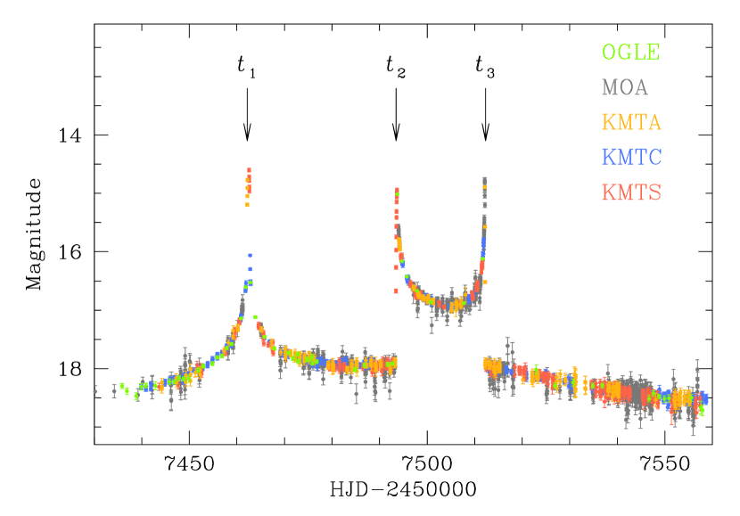
Figure 1.— Light curve of OGLE-2016-BLG-0156. The colors of data points correspond to those of telescopes, marked in the legend, used for observations. The times marked by arrows indicate the centers of the peaks at ${\rm HJD}^{\prime}={\rm HJD}-2450000\sim 7462.4$ ($t_{1}$), 7493.7 ($t_{2}$), and 7512.1 ($t_{3}$).

Photometry of the individual data sets are processed using the codes of the individual survey groups. All the photometry codes utilize the difference imaging technique developed by Alard & Lupton (1998). For the KMTC data set, we additionally conduct pyDIA photometry for the source color measurement. For the use of the multiple data sets reduced by different codes, we normalize the error bars of the individual data sets using the method described in Yee et al. (2012).

Figure 1 shows the light curve of OGLE-2016-BLG-0156. The light curve is characterized by three distinct peaks centered at ${\rm HJD}^{\prime}={\rm HJD}-2450000\sim 7462.4$ ($t_{1}$), 7493.7 ($t_{2}$), and 7512.1 ($t_{3}$). The peaks are widely separated with time gaps $\Delta t_{1-2}\sim 31.3$ days between the first and second peaks and $\Delta t_{2-3}\sim 18.4$ days between the second and the third peaks.

In Figure 2, we present the enlarged views of the individual peaks. It is found that the source became brighter by $\gtrsim 3$ magnitudes during very short periods of time, indicating that the peaks were produced by the source crossings over the caustic. Caustics produced by a binary lens form closed curves and thus caustic crossings usually occur in multiples of two. The region between the second and third peaks shows a U-shape pattern, which is the characteristic pattern appearing when the source passes inside a caustic, suggesting that the pair of the peaks centered at $t_{2}$ and $t_{3}$ were produced when the source star entered and exited the caustic, respectively. On the other hand, the first peak has no counterpart peak. Such a single-peak feature can be produced when the source crosses a caustic tip in which the gap between the caustic entrance and exit is smaller than the source size.

We note that all the peaks were densely covered. The first peak was covered by the combined data sets obtained using the three KMTNet telescopes, the second peak was resolved by the OGLE+KMTA data sets, and the last peak was covered by the MOA+KMTS data sets. The dense and continuous coverage of all the caustic crossings were possible thanks to the coordination of the high-cadence survey experiments using globally distributed telescopes.

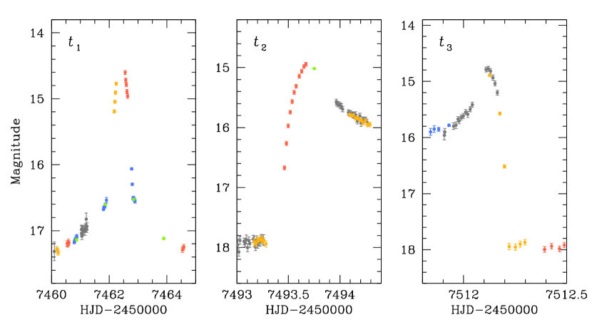
Figure 2.— Enlarged view of the three peaks in the lensing light curve. The locations of the individual peaks in the whole light curve are marked by $t_{1}$, $t_{2}$, and $t_{3}$ in Fig. 1.

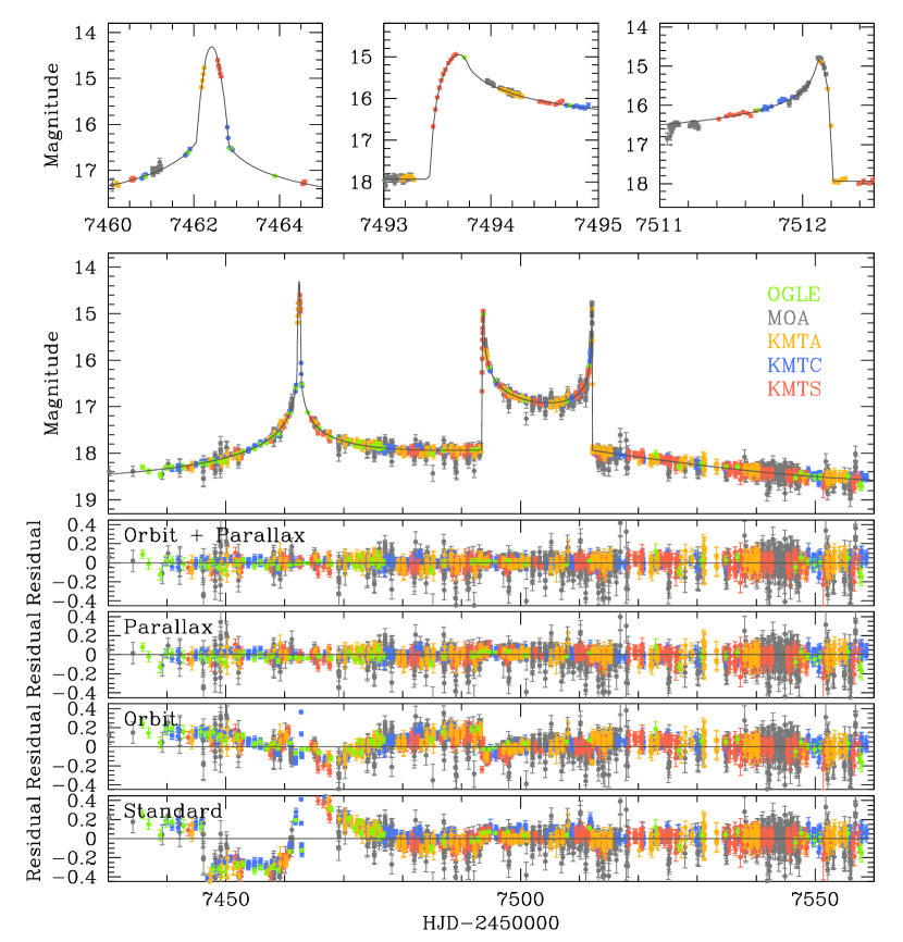
Figure 3.— The top two panels show the best-fit model light curve, the curve superposed on the data points, obtained by considering both the microlens-parallax and lens-orbital effects. The lower four panels compare the residuals of the 4 tested models. The ‘parallax’ and ‘orbit’ models are obtained by separately considering the microlens-parallax and lens-orbital effects. The ‘standard’ model consider neither of these higher-order effects.

3. Modeling Light Curve

3.1. Model under Rectilinear Relative Lens-Source Motion

The caustic-crossing features in the observed light curve indicates that the event is likely to be produced by a binary lens and thus we conduct binary-lens modeling of the light curve. We begin by searching for the sets of the lensing parameters that best explain the observed light curve under the assumption of the rectilinear lens-source motion, wherein the lensing light curve is described by 7 principal parameters. The first three parameters $(t_{0},u_{0},t_{\rm E})$ are identical to those of a single-lens events, describing the time of the closest lens-source approach, the separation at that time, and the event timescale, respectively. Because a binary lens is composed of two masses, one needs a reference position for the lens. We set the barycenter of the binary lens as the reference position. Due to the binary nature of the lens, one needs another three parameters $(s,q,\alpha)$, indicating the projected binary separation (normalized to $\theta_{\rm E}$), the mass ratio between the lens components, and the angle between the binary axis and the source trajectory, respectively. The last parameter $\rho$, which represents the ratio of the angular source radius $\theta_{*}$ to the angular Einstein radius, i.e., $\rho=\theta_{*}/\theta_{\rm E}$ (normalized source radius), is needed to describe the deviation of lensing magnifications caused by finite-source effects during caustic crossings.

Modeling the light curve is done through a multiple-step process. In the first step, we conduct a grid search for the parameters $s$ and $q$ and, for a given set of $s$ and $q$, the other parameters are searched for using a downhill approach based on the Markov Chain Monte Carlo (MCMC) method. We identify local solutions from the $\Delta\chi^{2}$ maps obtained from this preliminary search. In the second step, we refine the individual local solutions first by gradually narrowing down the parameter space and then allowing all parameters (including the grid parameters $s$ and $q$) to vary. If a satisfactory solution is not found from these searches, we repeat the process by changing the initial values of the parameters. We refer to the model based on these principal parameters as ‘standard model’.

From these searches, we find that it is difficult to find a lensing model that adequately describes the observed light curve. In the bottom panel of Figure 3 labeled as ‘standard’, we present the residual of the standard model. It shows that the model fit to the first peak is very poor although the model relatively well describes the second and third peaks.

3.2. Model with Higher-order Effects

The difficulty in finding a lensing model that fully explains all the features in the observed light curve under the assumption of the rectilinear lens-source motion suggests that the motion may not be rectilinear. This possibility is further supported by the long duration of the event.

Two major effects cause accelerations in the relative lens-source motion. One is the microlens-parallax effect. The other is the orbital motion of the lens: lens-orbital effect. We therefore conduct additional modeling considering these higher-order effects.

Incorporating the microlens-parallax effect into lensing modeling requires two additional parameters of $\pi_{{\rm E},N}$ and $\pi_{{\rm E},E}$. They represent the two components of the microlens-parallax vector $\mbox{\boldmath$\pi$}_{\rm E}$ directed to the north and east, respectively. The microlens-parallax vector is related to $\pi_{\rm rel}$, $\theta_{\rm E}$, and the relative lens-source proper motion vector $\mu$ by

$$\mbox{\boldmath$\pi$}_{\rm E}={\pi_{\rm rel}\over\theta_{\rm E}}{\mbox{\boldmath$\mu$}\over\mu}.$$ (4)

Considering the lens-orbital effect also requires additional parameters. Under the approximation that the positional changes of the lens components induced by the lens-orbital effect during the event is small, the effect is described by two parameters of $ds/dt$ and $d\alpha/dt$. They represent the change rates of the binary separation and the source trajectory angle, respectively.

We conduct a series of additional modeling runs considering the higher-order effects. In the ‘parallax’ and ‘orbit’ modeling runs, we separately consider the microlens-parallax and lens-orbital effects, respectively. In the ‘orbit+parallax’ modeling run, we simultaneously consider both the higher-order effects. For solutions considering microlens-parallax effects, it is known that there may exist a pair of degenerate solutions with $u_{0}>0$ and $u_{0}<0$ due to the mirror symmetry of the source trajectory with respect to the binary axis (Smith et al., 2003; Skowron et al., 2011). We inspect this ‘ecliptic degeneracy’ when microlens-parallax effects are considered in modeling.

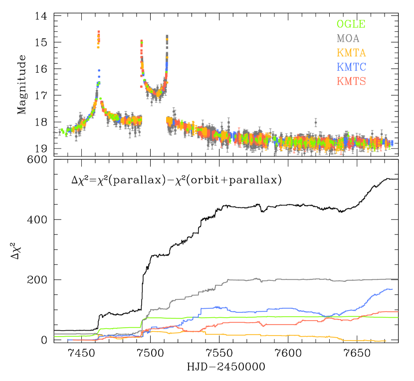
Figure 4.— Cumulative distribution of $\chi^{2}$ difference between the ‘parallax’ and ‘orbit+parallax’ models. The light curve in the upper panel is presented to show the region of the fit improvement.

Table 1Comparison of models

Model		$\chi^{2}$
Static		34436.4
Orbit		20019.4
Parallax	$u_{0}>0$	5749.4
–	$u_{0}<0$	6026.4
Orbit + parallax	$u_{0}>0$	5215.4
–	$u_{0}<0$	5221.2

In Table 1, we list the results of the individual modeling runs in terms of $\chi^{2}$ values of the fits. In order to visualize the goodness of the fits, we also present the residuals of the individual models in the lower panels of Figure 3. For the pair of solutions with $u_{0}>0$ and $u_{0}<0$ obtained considering microlens-parallax effects, we present the residuals of the solution yielding a better fit.

We compare the fits to judge the importance of the individual higher-order effects. From this, it is found that the major features of the light curve, i.e., the three peaks, still cannot be adequately explained by the orbital effect alone, although the effect improves fit by $\Delta\chi^{2}\sim 14407.0$ with respect to the standard model. See the residual labeled as ‘orbit’ in Figure 3. For the parallax model, on the other hand, the fit greatly improves, by $\Delta\chi^{2}\sim 28677.0$, and all the three peak features are approximately described. See the residual labeled as ‘parallax’ in Figure 3. We also find that the fit further improves, by $\Delta\chi^{2}\sim 534.0$ with respect to the parallax model, by additionally considering the lens-orbital effects. This indicates that although the lens-orbital effect is not the prime higher-order effects, it is important to precisely describe the light curve. Due to the relatively minor improvement, it is not easy to see the additional fit improvement by the lens-orbital effect from the comparison of the residuals of the ‘parallax’ and ‘orbit+parallax’ models. We, therefore, present the cumulative distribution of $\Delta\chi^{2}$ between the two models as a function of time in Figure 4. It is found that the fit improves throughout the event and major improvement occurs at the first and the second peaks and after the third peak. This indicates that the widely separated multiple peak features in the lensing light curve help to constrain the subtle higher-order effects. To check the consistency of the fit improvement, we also plot the distributions for the individual data sets. From the distributions, one finds that the $\chi^{2}$ improvement shows up in all data sets (OGLE, MOA, KMTC, and KMTS) except for the KMTA data set. We judge that the marginal orbital signal in the KMTA data set is caused by the relatively lower photometry quality than the other KMTNet data sets and the resulting smaller number of data points (626 points compared to 975 and 1214 points of the KMTS and KMTC data sets, respectively). We find the ecliptic degeneracy is quite severe although the model with $u_{0}>0$ is preferred over the model with $u_{0}<0$ by $\Delta\chi^{2}\sim 5.8$.

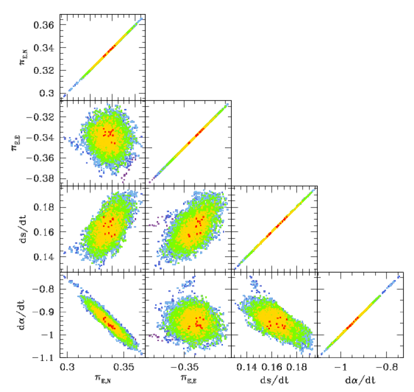
Figure 5.— Triangular diagram showing the $\Delta\chi^{2}$ distributions of MCMC points in the planes of the pair of the higher-order lensing lensing parameters $\pi_{{\rm E},N}$, $\pi_{{\rm E},E}$, $ds/dt$, and $d\alpha/dt$. Points marked in red, yellow, green, cyan, and blue represent those with $1\sigma$, $2\sigma$, $3\sigma$, $4\sigma$, and $5\sigma$, respectively.

Table 2Best-fit lensing parameters

parameter	$u_{0}>0$	$u_{0}<0$
$t_{0}$ (${\rm HJD}^{\prime}$)	7504.730 $\pm$ 0.012	7504.644 $\pm$ 0.015
$u_{0}$	0.083 $\pm$ 0.001	-0.085 $\pm$ 0.001
$t_{\rm E}$ (days)	68.19 $\pm$ 0.18	67.56 $\pm$ 0.39
$s$	0.727 $\pm$ 0.001	0.731 $\pm$ 0.002
$q$	0.869 $\pm$ 0.006	0.841 $\pm$ 0.006
$\alpha$ (rad)	1.408 $\pm$ 0.003	-1.408 $\pm$ 0.002
$\rho$ ($10^{-3}$)	0.615 $\pm$ 0.013	0.620 $\pm$ 0.012
$\pi_{{\rm E},N}$	0.334 $\pm$ 0.008	-0.347 $\pm$ 0.003
$\pi_{{\rm E},E}$	-0.335 $\pm$ 0.011	-0.406 $\pm$ 0.012
$ds/dt$ (yr-1)	0.168 $\pm$ 0.010	0.198 $\pm$ 0.013
$d\alpha/dt$ (yr-1)	-0.958 $\pm$ 0.039	1.059 $\pm$ 0.011
$I_{s,{\rm OGLE}}$	19.37 $\pm$ 0.01	19.37 $\pm$ 0.01
$I_{b,{\rm OGLE}}$	19.77 $\pm$ 0.01	19.77 $\pm$ 0.01

Note. — ${\rm HJD}^{\prime}={\rm HJD-2450000}$.

In Table 2, we present the lensing parameters of the best-fit models. Because the ecliptic degeneracy is severe, we present both the $u_{0}>0$ and $u_{0}<0$ solutions. Also presented are the $I$-band magnitudes of the source, $I_{s,{\rm OGLE}}$, and the blend, $I_{b,{\rm OGLE}}$, estimated based on the OGLE data. We note that the lensing parameters of the two solutions are roughly in the relation $(u_{0},\alpha,\pi_{{\rm E},N},d\alpha/dt)\leftrightarrow-(u_{0},\alpha,\pi_{{\rm E},N},d\alpha/dt)$ (Skowron et al., 2011). Several facts should noted for the obtained lensing parameters. First, the event timescale, $t_{\rm E}\sim 68$ days, is substantially longer than typical lensing events with $t_{\rm E}\sim 20$ days. Second, the binary parameters $(s,q)\sim(0.73,0.87)$ indicate that the lens is comprised of two similar masses with a projected separation slightly smaller than $\theta_{\rm E}$. Third, the normalized source radius $\rho\sim 0.62\times 10^{-3}$ is smaller by about a factor $\sim 2.5$ than the value of an event typically occurring on a star with a similar stellar type to the source of OGLE-2016-BLG-0156. Since $\rho=\theta_{*}/\theta_{\rm E}$, the small $\rho$ value suggests that the angular Einstein radius is likely to be big. Finally, the parameters describing the higher-order effects, i.e., $\pi_{{\rm E},N}$, $\pi_{{\rm E},E}$, $ds/dt$, and $d\alpha/dt$, are precisely determined with fractional uncertainties $\sim 2.4\%$, $3.3\%$, $6.3\%$, and $4.1\%$, respectively. In Figure 5, we present the $\Delta\chi^{2}$ distributions of MCMC points in the planes of the pair of the higher-order lensing parameters.

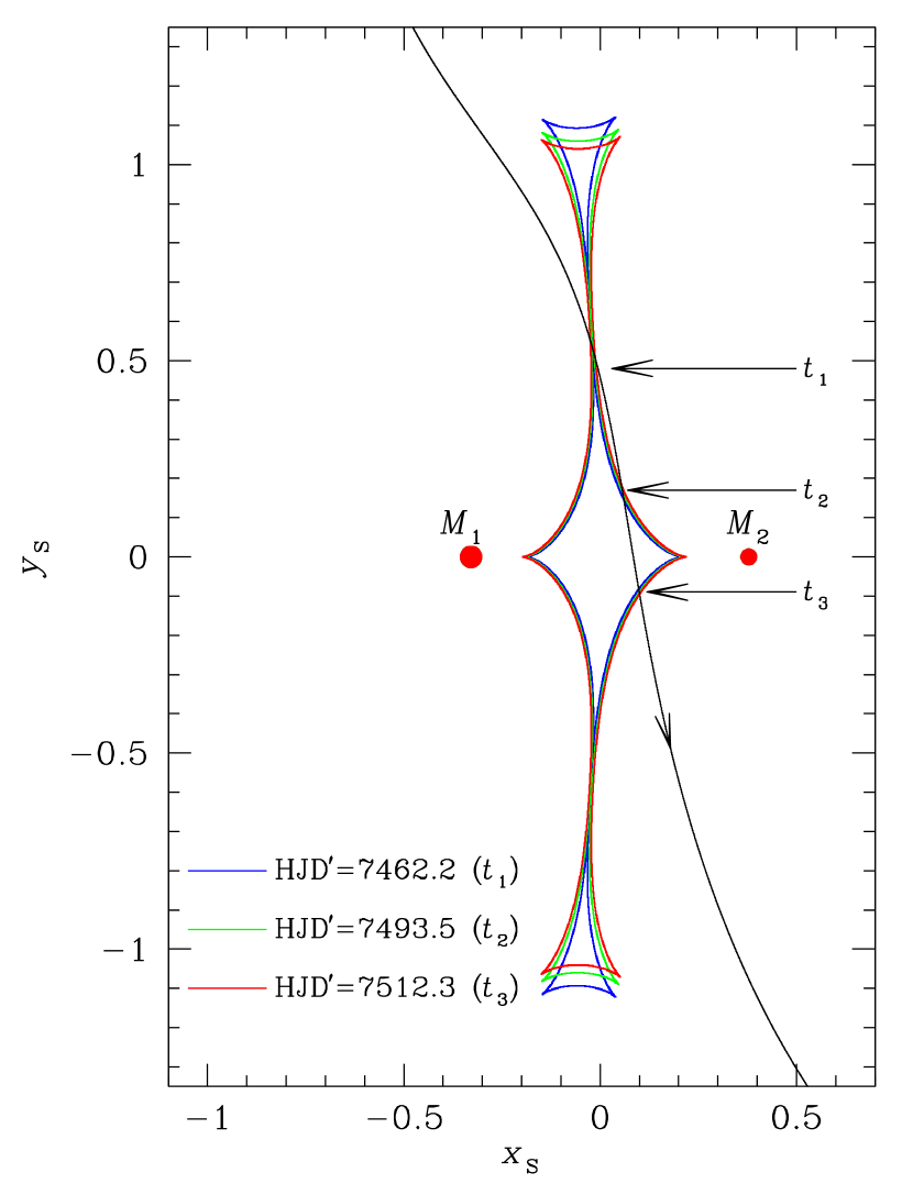
Figure 6.— Lens system configuration. The curve with an arrows represents the source trajectory with respect to the caustic (closed curve composed of concave segments). To show the variation of the caustic caused by the lens orbital motion, we present caustics at 3 moments corresponding to the times of the three peaks in the lensing light curve. We mark the positions of source crossings for the individual peaks occurring at $t_{1}$, $t_{2}$, and $t_{3}$. The small dots marked by $M_{1}$ and $M_{2}$ present the positions of the binary lens components. Lengths are scaled to the angular Einstein radius corresponding to the total mass of the lens.

In Figure 3, we present the model light curve, which is plotted over the data points, of the best-fit solution, i.e., the orbit+parallax model with $u_{0}>0$. In Figure 6, we present the corresponding lens-system configuration, showing the trajectory of the source with respect to the caustic. When the binary separation $s$ is close to unity, caustics form a single closed curve, ‘resonant caustic’, and as the separation becomes smaller, the caustic becomes elongated along the direction perpendicular to the binary axis and eventually splits into 3 segments, in which one 4-cusp central caustic is located around the center of mass and the other two triangular caustics are located away from the center of mass. (Erdl & Schneider, 1993; Dominik, 1999). For OGLE-2016-BLG-0156, the caustic topology corresponds to the boundary between the single closed-curve (‘resonant’) and triple closed-curve (‘close’) topologies. The source moved approximately in parallel with the elongated caustic, crossing the caustic 3 times at the positions marked by $t_{1}$, $t_{2}$, and $t_{3}$. The first peak was produced by the source crossing over the slim bridge part of the caustic connecting the 4-cusp central caustic and one of the triangular peripheral caustics. The peak could in principle have been produced by the source star’s approach to the the right cusp of the upper triangular caustic. We check this possibility and find that it cannot explain the light curve in the region around the first peak. The second and third peaks were produced when the source passed the upper and lower right parts of the central caustic, respectively.

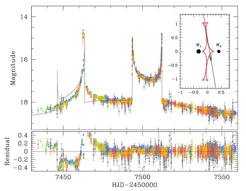
Figure 7.— Model light curve (curve superposed on data points) obtained under the assumption of the rectilinear relative lens-source motion. The lower panel shows the residual from the model. The inset in the upper panel shows the lens system configuration corresponding to the model.

We note that the well-covered 3-peak feature in the lensing light curve provides a very tight constraint on the source trajectory, and thus on the higher-order effects. To demonstrate the high sensitivity of the light curve to the slight change of the source trajectory induced by the higher-order effects, in Figure 7, we present the model fit of the standard solution and the corresponding lens system configuration. One finds that the straight source trajectory without higher-order effects can describe the second and third peaks by crossing similar parts of the central caustic to those of the solution obtained considering the higher-order effects. However, the extension of the trajectory crosses the upper triangular caustic, resulting in a light curve that differs greatly from the observed one. The importance of well-covered multiple peaks in determining $\mbox{\boldmath$\pi$}_{\rm E}$ was first pointed out by An & Gould (2001) and a good example was presented by Udalski et al. (2018) for the quintuple-peak lensing event OGLE-2014-BLG-0289.

4. Physical Lens Parameters

4.1. Angular Einstein Radius

For the unique determinations of the mass and distance to the lens, one needs to determine $\theta_{\rm E}$ as well as $\pi_{\rm E}$. See Equations (2) and (3). The angular Einstein radius is estimated from the combination of the normalized source $\rho$ and the angular source radius $\theta_{*}$ by $\theta_{\rm E}=\theta_{*}/\rho$. The $\rho$ value is determined from the light curve modeling. Then, one needs to estimate $\theta_{*}$ for the determination of $\theta_{\rm E}$.

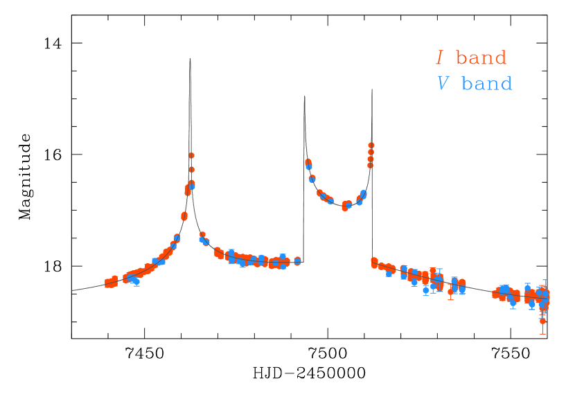
Figure 8.— KMTC $I$ and $V$-band data sets processed using the pyDIA photometry code. The data sets are used for the source color measurement.

We estimate the angular source radius from the de-reddened color, $(V-I)_{0}$, and brightness, $I_{0}$. For this, we first measure the instrumental (uncalibrated) source color and brightness from the KMTC $V$ and $I$-band data sets processed using the pyDIA photometry. We estimate the source color using the regression of the $V$ and $I$-band data sets. The color can also be estimated by using the model and we find that the source color estimated by both ways are consistent. Figure 8 shows the KMTC $I$ and $V$-band data. In the second step, following the method of Yoo et al. (2004), we calibrate the color and brightness of the source using the centroid of the red giant clump (RGC) in the color-magnitude diagram as a reference. In Figure 9, we mark the positions of the source, with $(V-I,I)=(1.99\pm 0.01,19.31\pm 0.01)$, and the RGC centroid, $(V-I,I)_{\rm RGC}=(2.43,15.98)$, in the instrumental color-magnitude diagram. With the known de-reddened color and brightness of the RGC centroid, $(V-I,I)_{{\rm RGC},0}=(1.06,14.46)$ (Bensby et al., 2011; Nataf et al., 2013), combined with the measured offsets in color, $\Delta(V-I)=-0.44$, and brightness, $\Delta I=3.33$, between the source and the RGC centroid, we estimate that the de-reddened color and brightness of the source star are $(V-I,I)_{0}=(V-I,I)_{0,{\rm RGC}}+\Delta(V-I,I)=(0.62\pm 0.01,17.78\pm 0.01)$, indicating that the source is a turn-off star. In the last step, we convert the measured $V-I$ into $V-K$ using the color-color relation of Bessell & Brett (1988) and then estimate the angular source radius using the relation between the color and surface brightness of Kervella et al. (2004). It is estimated that the angular source radius is

$$\theta_{*}=0.79\pm 0.06\ \mu{\rm as}.$$ (5)

In addition to the measurement error, the source color estimation is further affected by the uncertainty in determining RGC centroid and the differential reddening of the field. Bensby et al. (2013) showed that for lensing events in the fields with well defined RGCs, the typical error in the source color estimation is about 0.07 mag. We, therefore, estimate the errorbar of $\theta_{*}$ by considering this additional error.

The estimated angular Einstein radius is

$$\theta_{\rm E}=1.30\pm 0.09\ {\rm mas}.$$ (6)

For a typical lensing event produced by a low-mass star ($\sim 0.3~{}M_{\odot}$) located halfway between the source and observer ($D_{\rm L}\sim 4~{}{\rm kpc}$), the angular Einstein radius is $\theta_{\rm E}=\sqrt{\kappa M\pi_{\rm rel}}\sim 0.55~{}{\rm mas}~{}(M/0.3~{}M_{\odot})^{1/2}$. Then the estimated angular Einstein radius is $\gtrsim 2$ times bigger than the value of a typical lensing event. This is expected from the small value of the normalized source radius. Combined with the event timescale, the relative lens-source proper motion in the geocentric frame is estimated by

$$\mu_{\rm geo}={\theta_{\rm E}\over t_{\rm E}}=6.94\pm 0.69\ {\rm mas}\ {\rm yr}^{-1}.$$ (7)

The corresponding proper motion in the heliocentric frame is estimated by

$$\mu_{\rm helio}=\left|\mu_{\rm geo}{\mbox{\boldmath$\pi$}_{\rm E}\over\pi_{\rm E}}+{\bf v}_{\oplus,\perp}{\pi_{\rm rel}\over{\rm au}}\right|=5.94\pm 0.43\ {\rm mas}\ {\rm yr}^{-1}.$$ (8)

Here ${\bf v}_{\oplus,\perp}=(v_{\oplus,\perp,N},v_{\oplus,\perp,E})=(3.1,17.5)\ {\rm km}\ {\rm s}^{-1}$ denotes the projected velocity of Earth at $t_{0}$.

In Table 3, we summarize the estimated values of the angular Einstein radius, relative lens-source proper motion (in both geocentric and heliocentric frames), and the direction of the relative motion, i.e., $\phi=\tan^{-1}(\mu_{{\rm helio},E}/\mu_{{\rm helio},N})$. We also present the quantities resulting from the $u_{0}<0$ solution. The obtained quantities are slightly different from those of the $u_{0}>0$ solution due to the slight differences in $\rho$, $\pi_{{\rm E},N}$, and $\pi_{{\rm E},E}$.

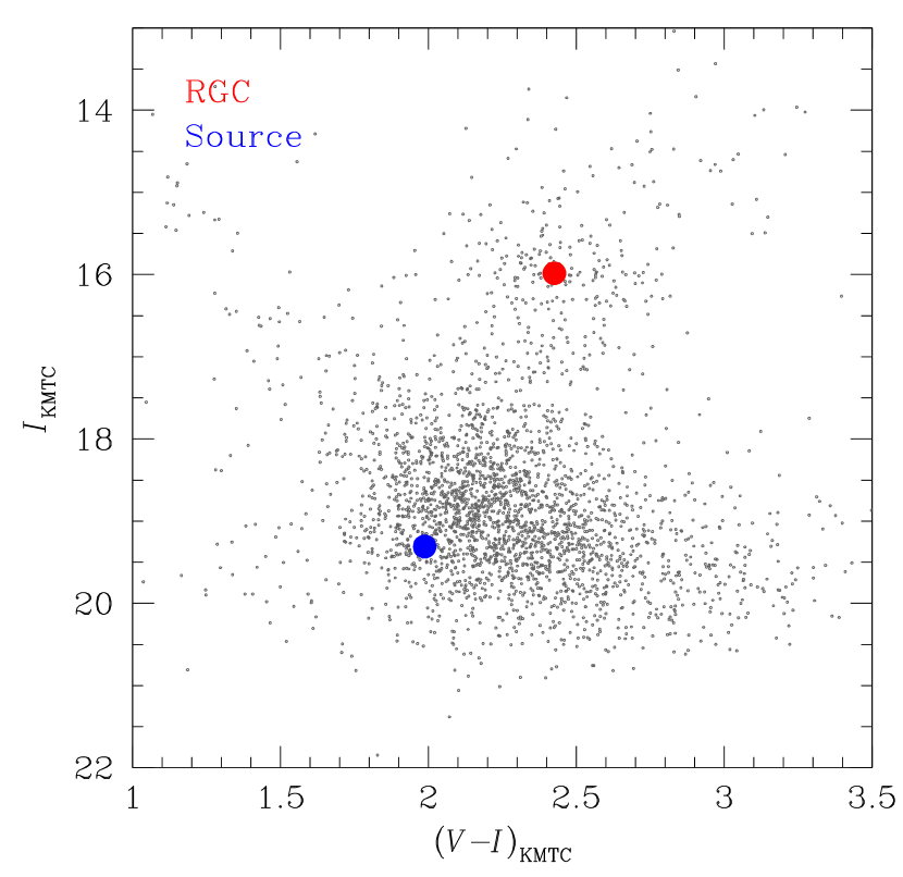
Figure 9.— Locations of the source and the centroid of red giant clump (RGC) in the instrumental color-magnitude diagram of stars around the source. The diagram is constructed using the pyDIA photometry of KMTC $I$ and $V$-band data.

Table 3Einstein radius and Proper Motion

Quantity	$u_{0}>0$	$u_{0}<0$
$\theta_{\rm E}$	$1.30\pm 0.09$	$1.28\pm 0.09$
$\mu_{\rm geo}$ (mas yr-1)	$6.94\pm 0.50$	$6.91\pm 0.50$
$\mu_{\rm helio}$ (mas yr-1)	$5.94\pm 0.43$	$4.88\pm 0.35$
$\phi$	$334^{\circ}$	$215^{\circ}$

4.2. Mass and Distance

With the measured $\pi_{\rm E}$ and $\theta_{\rm E}$, the masses of the individual lens components are determined as

$$M_{1}=0.18\pm 0.01\ M_{\odot},$$ (9)

and

$$M_{2}=qM_{1}=0.16\pm 0.01\ M_{\odot}.$$ (10)

It is estimated that the lens is located at a distance

$$D_{\rm L}=1.35\pm 0.09\ {\rm kpc}.$$ (11)

The determined masses and distance indicates that the lens is a binary composed of two M dwarfs located in the disk. The projected separation between the lens components is

$$a_{\perp}=s\theta_{\rm E}D_{\rm L}=1.28\pm 0.09\ {\rm au}.$$ (12)

We note that the $u_{0}<0$ solution yields similar lens parameters. In Table 4, we list the physical lens parameters for both the $u_{0}>0$ and $u_{0}<0$ solutions.

We check the validity of the solution by estimating the projected kinetic-to-potential energy ratio. We compute the ratio from the physical lens parameters of $M=M_{1}+M_{2}$ and $a_{\perp}$ and the measured lensing parameters of $s$, $\alpha$, $ds/dt$, and $d\alpha/dt$ by

$$\left({{\rm KE}\over{\rm PE}}\right)_{\perp}={(a_{\perp}/{\rm au})^{3}\over 8\pi^{2}(M/M_{\odot})}\left[\left({1\over s}{ds/dt\over{\rm yr}^{-1}}\right)^{2}+\left({d\alpha/dt\over{\rm yr}^{-1}}\right)^{2}\right].$$ (13)

In order for the lens system to be a gravitationally bound system, the solution should satisfy the condition of $({\rm KE}/{\rm PE})_{\perp}\leq{\rm KE}/{\rm PE}\leq 1.0$, where ${\rm KE}/{\rm PE}$ denotes the intrinsic energy ratio. The estimated ratio $({\rm KE}/{\rm PE})_{\perp}\sim 0.08$ satisfies this condition. The low value of the ratio suggests that the binary components are aligned along the line of sight.

4.3. Lens Brightness

Although the lens components are M dwarfs, they are located at a close distance, and the flux from the lens can comprise a significant portion of the blended flux, e.g., OGLE-2017-BLG-0039 (Han et al., 2018). To check this possibility, we estimate the expected brightness of the lens. The stellar types of the lens components are about M4.5V and M5.0V with absolute $I$-band magnitudes of $M_{I,1}\sim 10.5$ and $M_{I,2}\sim 11.0$ for the primary and companion, respectively, resulting in the combined magnitude $M_{I}\sim 10.0$. With the known distance to the lens, the de-reddened $I$-band magnitude is then $I_{L,0}=M_{I}+5\log D_{\rm L}-5\sim 20.6$. From the OGLE extinction map (Nataf et al., 2013), the total $I$-band extinction toward the source is $A_{I,{\rm tot}}\sim 1.48$. Assuming that about half of the total extinction is caused by the dust and gas located in front of the lens, i.e., $A_{I}\sim 0.7$, the expected brightness of the lens is

$$I_{\rm L}=I_{{\rm L},0}+A_{I}\sim 21.3.$$ (14)

Compared to the brightness of the blend, $I_{b,{\rm OGLE}}\sim 19.8$, it is found that the the flux from the lens comprises an important fraction, $\sim 25\%$, of the blended light. We note that the color constraint of the blended light cannot be used because the uncertainty of the $V$-band blend flux measurement is bigger than the flux itself.

Table 4Physical lens parameters

Parameter	$u_{0}>0$	$u_{0}<0$
$M_{1}$ ($M_{\odot}$)	$0.18\pm 0.01$	$0.16\pm 0.01$
$M_{2}$ ($M_{\odot}$)	$0.16\pm 0.01$	$0.13\pm 0.01$
$D_{\rm L}$ (kpc)	$1.35\pm 0.09$	$1.24\pm 0.08$
$a_{\perp}$ (au)	$1.28\pm 0.09$	$1.16\pm 0.08$
$({\rm KE}/{\rm PE})_{\perp}$	0.08	0.08

The bright nature of the lens combined with the high relative lens-source proper motion suggests that the lens can be directly observed from high-resolution follow-up observations. For the case of the lensing event OGLE-2005-BLG-169, the lens was resolved from the source on the Keck AO images when they were separated by $\sim 50$ mas after $\sim 8$ years after the event (Batista et al., 2015). By applying the same criterion, the lens and source of OGLE-2016-BLG-0156 can be resolved if similar follow-up observations are conducted $\sim 6$ years after the event, i.e., after 2022. For the case of the another lensing event OGLE-2012-BLG-0950, Bhattacharya et al. (2018) resolved the source and lens using Keck and the Hubble Space Telescope when they were separated by $\sim 34$ mas. According to this criterion, then, the source and lens of this event would be resolved in 2022.

Because follow-up observations are likely to to be conducted in near infrared bands, we estimate the expected $H$-band brightness of the lens. The absolute $H$-band magnitudes of the individual lens components are $M_{H}\sim 8.2$ and 8.7 resulting in the combined brightness of $M_{H,0}\sim 7.7$. With $A_{I}=A_{I,{\rm tot}}/2\sim 0.7$ and $E(V-I)=E_{\rm tot}(V-I)/2\sim 0.6$ from Nataf et al. (2013) and adopting the relation $A_{H}\sim 0.108A_{V}\sim 0.14$ of Nishiyama et al. (2008), we estimate that $H$-band brightness of the lens is

$$H_{\rm L}=M_{H,0}+A_{H}+5\log D_{\rm L}-5\sim 17.9.$$ (15)

The $H$-band brightness of the source is

$$H_{\rm S}=I_{\rm S}-E(I-H)-(I-H)_{0}\sim 17.5,$$ (16)

which is similar to that of the the lens. When the lens brightness is similar to the brightness of the source, the lens and source can be better resolved as demonstrated for events OGLE-2005-BLG-169 (Bennett et al., 2015), MOA-2008-BLG-310 (Bhattacharya et al., 2017), and OGLE-2012-BLG-0950 (Bhattacharya et al., 2018).

5. Conclusion

We analyzed a binary microlensing event OGLE-2016-BLG-0156. We found that the light curve of the event exhibited pronounced deviations induced by higher-order effects, especially the microlens effect. It is found that the multiple-peak feature provided a very tight constraint on the microlens-parallax measurement. In addition, the good coverage of all the peaks from the combined survey observations allowed us to precisely measure the angular Einstein radius. We uniquely determined the physical lens parameters from the measured values of $\pi_{\rm E}$ and $\theta_{\rm E}$ and found that the lens was a binary composed of two M dwarfs located in the disk. We also found that the flux from the lens comprises an important fraction of the blended flux. The bright nature of the lens combined with the high relative lens-source motion suggested that the lens could be directly observed from high-resolution follow-up observations.

References

- Alard & Lupton (1998) Alard, C., & Lupton, R. H. 1998, ApJ, 503, 325
- Albrow (2017) Albrow, M. 2017, MichaelDAlbrow/pyDIA: Initial Release on Github, doi: 10.5281/zenodo.268049
- An & Gould (2001) An, J. H., & Gould, A. 2001, ApJ, 563, L11
- Batista et al. (2015) Batista, V., Beaulieu, J.-P., Bennett, D. P., et al. 2015, ApJ, 808, 170
- Bennett et al. (2015) Bennett, D. P., Bhattacharya, A., Anderson, J., et al. 2015, ApJ, 808, 169
- Bensby et al. (2011) Bensby, T., Adén, D., Meléndez, J., et al. 2011, PASP, 533, 134
- Bensby et al. (2013) Bensby, T., Yee, J. C., Feltzing, S., et al. 2013, A&A, 549, 147
- Bessell & Brett (1988) Bessell, M. S., & Brett, J. M. 1988, PASP, 100, 1134
- Bhattacharya et al. (2017) Bhattacharya, A., Bennett, D. P., Anderson, J., et al. 2017, AJ, 154, 59
- Bhattacharya et al. (2018) Bhattacharya, A., Beaulieu, J. P., Bennett, D. P. 2018, AJ, 156, 289
- Bond et al. (2001) Bond, I. A., Abe, F., Dodd, R. J., et al. 2001, MNRAS, 327, 868
- Bramich et al. (2013) Bramich, D. M., Horne, K., Albrow, M. D., et al. 2013, MNRAS, 428, 2275
- Calchi Novati et al. (2015) Calchi Novati, S., Gould, A., Udalski, A., et al. 2015, ApJ, 804, 20
- Dong et al. (2007) Dong, Subo, Udalski, A., Gould, A., et al. 2007, ApJ, 664, 862
- Dominik (1999) Dominik, M. 1999, A&A, 349, 108
- Erdl & Schneider (1993) Erdl, H., & Schneider, P. 1993, A&A, 268, 453
- Gould (1992) Gould, A. 1992, ApJ, 392, 442
- Gould (1994a) Gould, A. 1994a, ApJ, 421, L71
- Gould (1994b) Gould, A. 1994b, ApJ, 421, L75
- Gould (2000) Gould, A. 2000, ApJ, 542, 785
- Han et al. (2018) Han, C., Jung, Y. K., Udalski, A., et al. 2018, ApJ, 867, 136
- Jaroszyński & Mao (2001) Jaroszyński, M., & Mao, S. 2001, MNRAS, 325, 1546
- Kervella et al. (2004) Kervella, P., Thévenin, F., Di Folco, E., & Ségransan, D. 2004, A&A, 426, 297
- Kim et al. (2016) Kim, S.-L., Lee, C.-U., Park, B.-G., et al. 2016, JKAS, 49, 37
- Muraki et al. (2011) Muraki, Y., Han, C., Bennett, D. P., et al. 2011, ApJ, 741, 22
- Nataf et al. (2013) Nataf, D. M., Gould, A., Fouqué, P., et al. 2013, ApJ, 769, 88
- Nemiroff & Wickramasinghe (1994) Nemiroff, R. J., & Wickramasinghe, W. A. D. T. 1994, ApJ, 424, L21
- Nishiyama et al. (2008) Nishiyama, S., Nagata, T., Tamura, M., et al. 2008, ApJ, 680, 1174
- Refsdal (1966) Refsdal, S. 1966, MNRAS, 134, 315
- Skowron et al. (2011) Skowron, J., Udalski, A., Gould, A., et al. 2011, ApJ, 738, 87
- Smith et al. (2003) Smith, M. C., Mao, S., & Paczyński, B. 2003, MNRAS, 339, 925
- Sumi et al. (2003) Sumi, T., Abe, F., Bond, I. A., et al. 2003, ApJ, 591, 20
- Yee et al. (2012) Yee, J. C., Shvartzvald, Y., Gal-Yam, A., et al. 2012, ApJ, 755, 102
- Yoo et al. (2004) Yoo, J., DePoy, D. L., Gal-Yam, A., et al. 2004, ApJ, 603, 139
- Udalski et al. (2018) Udalski, A., Han, C., Bozza, V., et al. 2018, ApJ, 853, 70
- Udalski et al. (2015a) Udalski, A., Szymański, M. K., & Szymański, G. 2015a, AcA, 65, 1
- Udalski et al. (2015b) Udalski, A., Yee, J. C., Gould, A. 2015b, ApJ, 799, 237
- Witt & Mao (1994) Witt, H. J., & Mao, S. 1994, ApJ, 430, 505