Holographic Phase Retrieval and Reference Design

Abstract

A general mathematical framework and recovery algorithm is presented for the holographic phase retrieval problem. In this problem, which arises in holographic coherent diffraction imaging, a “reference” portion of the signal to be recovered via phase retrieval is a priori known from experimental design. A generic formula is also derived for the expected recovery error when the measurement data is corrupted by Poisson shot noise. This facilitates an optimization perspective towards reference design and analysis. We employ this optimization perspective towards quantifying the performance of various reference choices.

1 Introduction

1.1 Phase Retrieval and Coherent Diffraction Imaging

The phase retrieval problem concerns recovering a signal from the squared magnitude of its Fourier transform. The problem can be stated symbolically as

$$\begin{split}&\textbf{Given}\quad\big{|}\widehat{X}(\omega)\big{|}^{2}\doteq\left|\int_{t\in T}X(t)e^{-i\omega t}\right|^{2}\quad\text{for}\;\omega\in\Omega\\ &\textbf{Recover}\quad X\end{split},$$ (1.1)

where $T$ and $\Omega$ are the (possibly multidimensional) domains of the signal and its Fourier transform, respectively. Phase retrieval arises ubiquitously in scientific imaging, where one seeks to “image" or determine the structure of an object from various phaseless data measurements. Such settings include crystallography [Mil90], diffraction imaging [BDP⁺07], optics [Wal63], and astronomy [DF87].

Phase retrieval has gained enormous attention over the last two decades, largely due to an emerging imaging technique known as Coherent Diffraction Imaging, or CDI [MCKS99] (illustrated in Fig. 1). In CDI, a coherent beam source, often being an X-ray, is illuminated upon a sample of interest. Upon the beam reaching the sample, diffraction occurs and secondary electromagnetic waves are emitted which travel until reaching a far-field detector. The detector measures the photon flux and hence records the resulting diffraction pattern, which is approximately proportional to the squared magnitude of the Fourier transform of the electric field of the sample. One can, in principle, recover the structure of the sample from the diffraction pattern by solving the phase retrieval problem [Goo17, Jag16, SEC⁺15]. With the advent of extremely powerful X-ray light sources, such as X-ray Free-Electron Lasers (XFELs) [CBB⁺06] and synchrotron radiation [RVW⁺01], CDI is pushing the frontier of high-resolution imaging of biological and material specimens at the nanoscale [LZGJ⁺18, XMR⁺14, LHM⁺12, MIRM15].

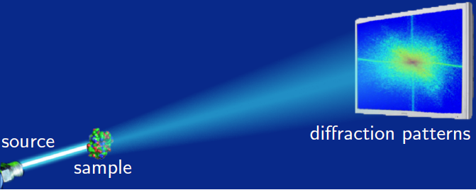
Figure 1: CDI setup. Image courtesy of [CLS15b].

1.2 Phase Retrieval Algorithms

The phase retrieval problem does not admit a unique solution, as the forward mapping in Eq. 1.1 maps signals related by certain intrinsic symmetries to the same set of measurements (these are discussed in detail in Section 2.1). Also, modulo these unavoidable ambiguities, there still may not be a unique solution. This nonuniqueness occurs frequently for one-dimensional signals, but only on a set of (Lebesgue) measure zero for two- or higher-dimensional signals [Hay82, SEC⁺15, BBE17, SC91]. Thus, for CDI experiments (which concern two- or three-dimensional signals), there is almost surely a unique solution up to the intrinsic ambiguities. Nevertheless, solving the problem is equivalent to solving a quadratic system—which is well known to be NP-hard [BTN01].

In practice, the phase retrieval problem is often cast as a nonconvex optimization problem, for which various alternating-projection type algorithms are commonly employed. The most notable one is Fienup’s Hybrid Input-Output (HIO) algorithm [Fie78]. Other practical variants include Relaxed Averaged Alternating Reflections (RAAR) [Luk05], Difference Map [ERT07], and Alternating Direction Method of Multipliers (ADMM) [WYLM12, BPC⁺11, BS17]. While often successful, these algorithms are not guaranteed to find the correct solution. They are also known to suffer from various problems such as stagnation at erroneous solutions, slow runtime, sensitivity to noise and parameter tuning [Mar07, Els03].

To mitigate these difficulties, a line of recent work has proposed to modify the typical CDI setup. This involves sequentially modulating either the beam pattern or the Fourier transform via random or deterministic masks, thereby gathering multiple-shot measurements [LCL⁺08, JJB⁺08, CLS15b, JEH15, JEH16]. Several of these proposals have resulted in efficient algorithms with provable guarantees [CLS15b, CLS15a, JEH15]. However, such a multiple-shot experiment is largely impractical, as the specimen could be damaged before the measurement process is complete [SEC⁺15].

1.3 Holographic CDI and Holographic Phase Retrieval

In this paper, we consider another variant of CDI based on the holographic idea introduced by Gabor in 1948 [Gab48], which we shall term as holographic CDI. In holographic CDI, the experiment remains single-shot, but a “reference” area, whose structure is a priori known, is included in the diffraction area alongside the sample of interest (see Fig. 2 for the system setup and Fig. 3 for a schematic illustration).

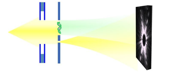
Figure 2: Holographic CDI setup. Image courtesy of [SLLF12].

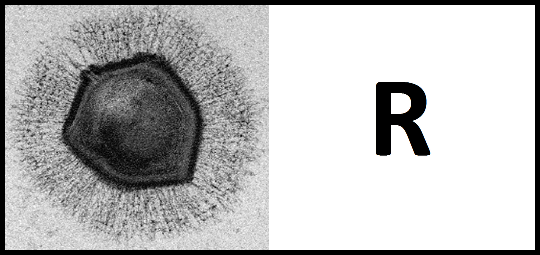
Figure 3: The diffraction area in Holographic CDI contains an unknown specimen (here shown as a mimivirus  [GKL⁺08]) together with a known reference (here shown as “$\mathbf{\mathrm{R}}$”). Popular choices for the reference $\mathbf{\mathrm{R}}$ are shown in Fig. 4.

Introducing a reference substantially simplifies the resulting phase retrieval problem, which we call holographic phase retrieval: the computational problem is now a linear deconvolution, which is equivalent to solving a linear system [KAKK72, ELS⁺04, GSF07, MA08, KH90]. The entailing computation can be further streamlined when certain specific reference shapes are employed. Due to its simplicity, holographic CDI is growing in its impact and popularity [GO18, SLLF12].

In the imaging community, popular reference choices are the pinhole reference [LU62, KH90], the slit reference [GSF07, GSF08, ZO10], and the block reference [PPP07, BSLL18, MA08], as illustrated in Fig. 4.

(a) Pinhole reference

(b) Slit reference

(c) Block reference

Figure 4: Schematic of the three leading reference choices for Holographic CDI. (Images have $16\times 16$ enlarged pixels for illustration.)

Other proposed references include L-shapes [GSF07], parallelograms [GSF07], and annuluses [GO18], and Uniformly Redundant Arrays [MBS⁺08]. These reference shapes are typically realized as “empty space” cut out from a surrounding metal apparatus (see, e.g., Fig. 2). For signal recovery using these references, reference-specific algorithms—which take a different approach than linear deconvolution and only apply to small classes of references—have been proposed [GSF07]. Moreover, studies of these methods have to date been almost entirely empirical. Some error analysis is provided in [WTT⁺16].

1.4 Our Contributions

In this paper, we derive a general mathematical framework for holographic phase retrieval, encompassing the problem’s setup, recovery algorithm, and error analysis.

• Firstly, we formulate the holographic phase retrieval problem for a general specimen and reference setup. We then provide a recovery algorithm, termed Referenced Deconvolution, which essentially amounts to solving a structured linear system. We then further show how particular reference choices simplify this linear system. This provides a novel perspective on why fast, specialized algorithms (e.g., see [LU62, PPP07, GSF07]) can be designed for these reference choices.

• We derive a formula for the expected recovery error given noise-corrupted data. This formula offers a quantitative metric for experimental design and simulation, and allows for viewing the problem of reference design from an optimization perspective. This formula is then specialized to the Poisson shot noise, which occurs intrinsically in CDI due to quantum mechanical principles. This leads to the key notion of the reference scaling factor, based on which we characterize the popular references. In particular, the pinhole reference (Fig. 4(a)) is a good choice for “flat-spectrum” data, whereas the block reference (Fig. 4(c)) is well suited for low-frequency dominant data.

Numerical results demonstrate the power of the proposed referenced deconvolution method and the advantage of the block reference for recovering typical CDI imaging specimens. We also view this work as a means to introduce the holographic phase retrieval problem and the optimal reference design problem to a wider mathematical and scientific audience.

1.5 Paper Organization

Section 2 introduces the holographic phase retrieval problem and the referenced deconvolution algorthm. The special cases of popular reference choices are then further studied. Section 3 introduces an error analysis framework for holographic phase retrieval and the referenced deconvolution algorithm. This is further specialized to Poisson shot noise. The notion of a reference scaling factor is introduced, and is shown to play a key role in analyzing the expected Poisson noise error resulting from a given reference choice. Specific error analysis is then provided for popular reference choices, and is used to compare their performance. Section 4 presents the results of numerical simulations.

2 Holographic Phase Retrieval and Referenced Deconvolution

The phase retrieval problem is introduced in Section 2.1. The holographic phase retrieval problem and the Referenced Deconvolution algorithm are then introduced in Section 2.2 and Section 2.3, respectively. Then, the algorithm and resulting linear system are specialized to the three popular reference choices in Section 2.4.

2.1 The Phase Retrieval Problem

We consider the discrete two-dimensional phase retrieval problem. This discrete setting is manifested in practical CDI experiments, since CCD detectors can only take measurements at a finite number of pixel locations.

For a signal $X\in\mathbb{C}^{n_{1}\times n_{2}}$, let $\widehat{X}$ be the size $m_{1}\times m_{2}$ discrete Fourier transform of $X$ given by

$$\widehat{X}(k_{1},k_{2})=\sum_{t_{1}=0}^{n_{1}-1}\sum_{t_{2}=0}^{n_{2}-1}X(t_{1},t_{2})e^{-2\pi i(t_{1}k_{1}/m_{1}+t_{2}k_{2}/m_{2})},\quad k_{1}\in\left\{0,\dots,m_{1}-1\right\},k_{2}\in\{0,\dots,m_{2}-1\}.$$ (2.1)

Whenever $m_{1}>n_{1}$ and $m_{2}>n_{2}$, the Fourier transform is injective and is said to be oversampled. The mapping can also be compactly expressed as matrix multiplication:

$$\widehat{X}=F_{L}XF_{R}^{T},$$ (2.2)

where $F_{L}\in\mathbb{C}^{m_{1}\times n_{2}}$ and $F_{R}\in\mathbb{C}^{m_{2}\times n_{2}}$ are the corresponding discrete Fourier transform (DFT) matrices given by

$$F_{L}(k,t)=e^{-2\pi ikt/m_{1}} \quad\text{for}\;\left(k,t\right)\in\{0,\dots,m_{1}-1\}\times\{0,\dots,n_{1}-1\},$$

$$F_{R}(k,t)=e^{-2\pi ikt/m_{2}} \quad\text{for}\;\left(k,t\right)\in\{0,\dots,m_{2}-1\}\times\{0,\dots,n_{2}-1\}.$$

When $m_{1}\geq n_{2}$ and $m_{2}\geq n_{2}$, both $F_{L}$ and $F_{R}$ have mutually orthogonal columns, and so the inverse mapping is given simply by

$$X=\frac{1}{m_{1}m_{2}}F_{L}^{*}\widehat{X}(F_{R}^{*})^{T}.$$ (2.3)

The forward and inverse transforms in Eqs. 2.2 and 2.3 can also be conveniently expressed as a single matrix multiplication based on matrix Kronecker products. Let $\operatorname{vec}(\cdot)$ be the columnwise vectorization operator acting on matrices and $\otimes$ denote the matrix Kronecker products. The following result can be directly verified:

Lemma 2.1.

$Y=AXB\Longleftrightarrow\operatorname{vec}(Y)=(B^{T}\otimes A)\operatorname{vec}(X)$.

Applying Lemma 2.1 to Eqs. 2.2 and 2.3 gives

$$\operatorname{vec}(\widehat{X}) =(F_{R}\otimes F_{L})\operatorname{vec}(X),$$ (2.4)

$$\operatorname{vec}(X) =\frac{1}{m^{2}}(F_{R}^{*}\otimes F_{L}^{*})\operatorname{vec}(\widehat{X}),\quad\text{when}\;m_{1}\geq n_{1}\;\text{and}\;m_{2}\geq n_{2}.$$ (2.5)

We are now ready to define the phase retrieval problem in the two-dimensional, discrete setting.

Definition 2.2.

The (Fourier) phase retrieval problem consists of recovering a signal $X\in\mathbb{C}^{n_{1}\times n_{2}}$ given the squared magnitudes of its Fourier transform values, i.e. given the set of values $|\widehat{X}(k_{1},k_{2})|^{2},k_{1}\in\{0,\ldots,m_{1}-1\},k_{2}\in\{0,\ldots,m_{2}-1\}$, which shall be denoted as $|\widehat{X}(k_{1},k_{2})|^{2}$.

Here, exact recovery is not possible, as the mapping $X\mapsto|\widehat{X}|^{2}$ is not injective due to the following intrinsic ambiguities:

1. Global phase shift: if $X\mapsto|\widehat{X}|^{2}$, then $e^{i\theta}X\mapsto|\widehat{X}|^{2}$ for any $\theta\in[0,2\pi)$;

2. Conjugate-flipping: if $X\mapsto|\widehat{X}|^{2}$, then $X^{\prime}\mapsto|\widehat{X}|^{2}$ for $X^{\prime}\in\mathbb{C}^{n_{1}\times n_{2}}$ with $\overline{X(n_{1}-1-t_{1},n_{2}-1-t_{2})}=X^{\prime}(t_{1},t_{2})$ for all $t_{1},t_{2}$.

As well, circular shifts of $X$ also produce the same set of measurements if no nonzero entries are shifted past the signal domain boundaries. This gives a third intrinsic ambiguity for signals $X$ which have zero rows or columns at their boundaries. Taking all possible compositions of these operations forms a set (in fact, an equivalence class) of signals which are “physically equivalent” to $X$ and have exactly the same magnitude measurements $|\widehat{X}|^{2}$. Thus, recovering $X$ from $|\widehat{X}|^{2}$ shall be understood as recovery up to these symmetries.

Definition 2.3.

For signals $X_{1},X_{2}\in\mathbb{C}^{n_{1}\times n_{2}}$ both indexed over $\left\{0,1,\dots,n_{1}-1\right\}\times\left\{0,1,\dots,n_{2}-1\right\}$, the cross-correlation $C_{[X_{1},X_{2}]}\in\mathbb{C}^{(2n_{1}-1)\times(2n_{2}-1)}$ between $X_{1}$ and $X_{2}$ is defined as

$$C_{[X_{1},X_{2}]}(s_{1},s_{2})=\sum_{t_{1}=0}^{n_{1}-1}\sum_{t_{2}=0}^{n_{2}-1}X_{1}(t_{1},t_{2})\overline{X_{2}(t_{1}-s_{1},t_{2}-s_{2})},$$ (2.6)

for $\left(s_{1},s_{2}\right)\in\{-(n_{1}-1),\dots,n_{1}-1\}\times\left\{-\left(n_{2}-1\right),\dots,n_{2}-1\right\}$, where any $X_{1}(t_{1},t_{2})$ or $X_{2}(t_{1}-s_{1},t_{2}-s_{2})$ in the summands that are outside the valid index range are taken as $0$.

When $X_{1}$ and $X_{2}$ are both equal to the same signal $X$, $C_{[X_{1},X_{2}]}$ is known as the autocorrelation of $X$, and is denoted by $A_{X}$. Let $\widehat{X}$ be the size $m_{1}\times m_{2}$ Fourier transform of $X$. It is well-known that [OS09]

$$|\widehat{X}|^{2}=\widehat{A_{X}},$$ (2.7)

where

$$\begin{split}\widehat{A_{X}}=F_{LA}A_{X}F_{RA}^{T}\quad\text{with}\;F_{LA}\in\mathbb{C}^{m_{1}\times(2n_{1}-1)},m_{1}\geq 2n_{1}-1\quad F_{RA}\in\mathbb{C}^{m_{2}\times(2n_{2}-1)},m_{2}\geq 2n_{2}-1\\ \text{and}\;F_{LA}(k,t)=e^{-2\pi ikt/m_{1}}\;\forall\;(k,t)\in\{0,\dots,m_{1}-1\}\times\{-(n_{1}-1),\dots,n_{1}-1\},\\ \text{and}\;F_{RA}(k,t)=e^{-2\pi ikt/m_{2}}\;\forall\;(k,t)\in\{0,\dots,m_{2}-1\}\times\{-(n_{2}-1),\dots,n_{2}-1\}.\end{split}$$ (2.8)

Moreover, if $m_{1}\geq 2n_{1}-1$ and $m_{2}\geq 2n_{2}-1$, the mapping $A_{X}\mapsto\widehat{A_{X}}$ is injective, and hence $A_{X}$ can be recovered from $\widehat{A_{X}}$, or equivalently $|\widehat{X}|^{2}$, by the corresponding inverse transform:

$$A_{X}=\frac{1}{m_{1}m_{2}}F_{LA}^{*}|\widehat{X}|^{2}(F_{RA}^{*})^{T}.$$ (2.9)

Namely, $A_{X}$ is uniquely determined from the $m_{1}\geq 2n_{1}-1,m_{2}\geq 2n_{2}-1$ uniform frequency sampling points. The entire frequency spectrum is in turn determined by taking the 2D discrete-time Fourier transform of $A_{X}$. Thus, any oversampling past the $m_{1}=2n_{1}-1,m_{2}=2n_{2}-1$ threshold provides no additional information. This is in some sense the phase retrieval analogue of the Shannon sampling theorem [CESV15].

A powerful result by Hayes [Hay82] establishes that for all two- or higher-dimensional signals, excluding a set of Lebesgue measure zero, the only transformations on $X$ which preserve $|\widehat{X}|^{2}$ are the physically equivalent symmetries discussed above. Thus, phase retrieval is generally well-posed in two or higher dimensions.

2.2 Holographic Phase Retrieval and Deconvolution

For simplicity of exposition, henceforth we focus on square $X\in\mathbb{C}^{n\times n}$. Suppose a reference $R\in\mathbb{C}^{n\times n}$ of the same size is situated on the right next to $X$, i.e., as illustrated in Fig. 3. This gives $[X,R]\in\mathbb{C}^{n\times 2n}$ defined by

$$[X,R](t_{1},t_{2})=\begin{cases}X(t_{1},t_{2})&\quad t_{2}\in\{0,\dots,n-1\}\\ R(t_{1},t_{2})&\quad t_{2}\in\{n,\dots,2n-1\}.\end{cases}$$

We may assume without loss of generality that the magnitudes of the entries of $X$ and $R$ are within the interval $[0,1]$. This convention has the physical interpretation of indicating the (average) transmission coefficient of the specimen at each pixel location. Roughly speaking, the transmission coefficient measures the fraction of incident electromagnetic radiation that is transmitted, rather than being reflected or absorbed and is a material property—Fig. 5 shows the transmission coefficient of polycarbonate at different photon energy levels. We shall subsequently consider reference setups that are physically realized as shapes cut from a surrounding opaque apparatus (i.e. consisting of metal that blocks all incident radiation). For the opaque part, the transmission coefficient is $0$, whereas for the cut-out part the coefficient is $1$.

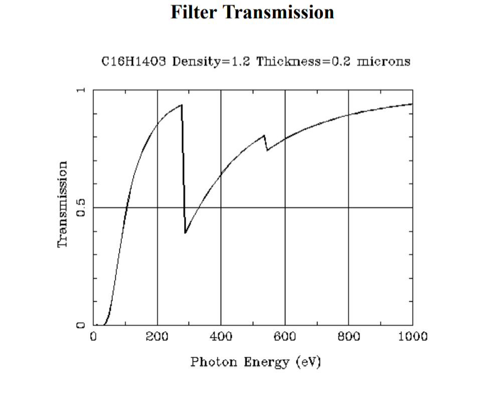
Figure 5: Transmission coefficient of polycarbonate at different photon energies  [The10].

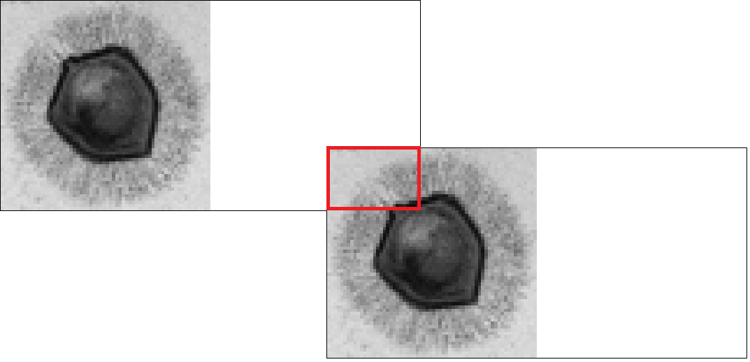
(a)

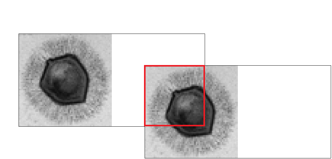
(b)

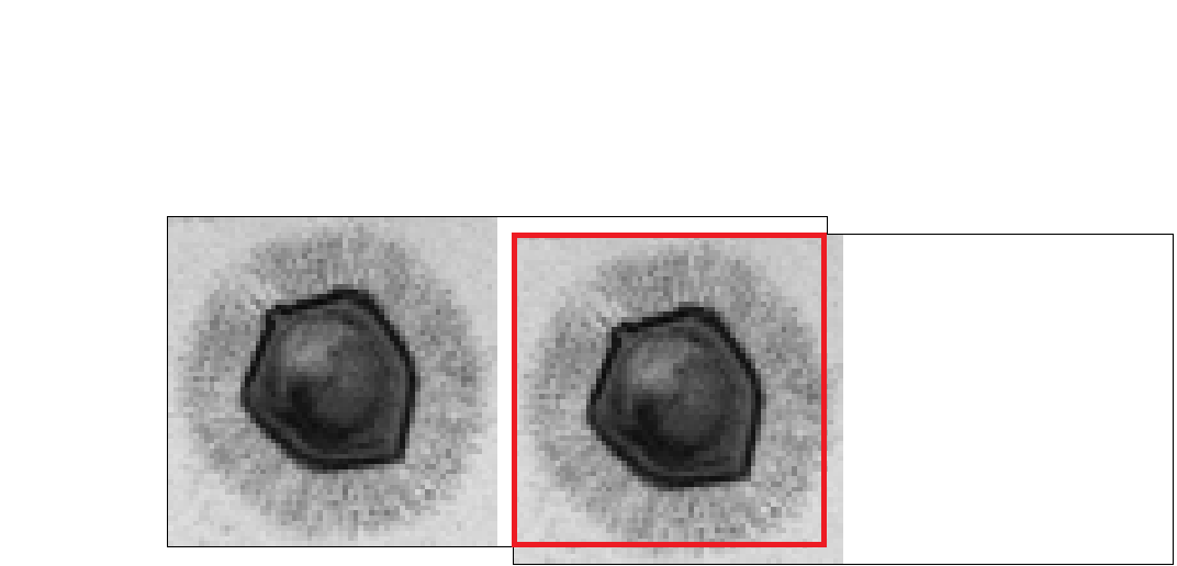
(c)

Figure 6: Near the boundary of the index range, each successive autocorrelation value of $[X,R]$ is formed by the overlap of a subregion of $X$ with a subregion of $R$, which effectively gives a new linear measurement of $X$, as $R$ is known. The original image $X$ can then be recovered via solving the linear system in Eq. 2.12.

In the above setting, the holographic phase retrieval problem is:

Holographic phase retrieval: given $R\in\mathbb{C}^{n\times n}$ and $|\widehat{\left[X,R\right]}|^{2}\in\mathbb{R}^{m_{1}\times m_{2}}$, recover $X\in\mathbb{C}^{n\times n}$.

Henceforth we assume $m_{1}=m_{2}=m$ with $m\geq 4n-1$. We can then recover the autocorrelation of $\left[X,R\right]$, $A_{\left[X,R\right]}$, by taking the inverse Fourier transform on $|\widehat{\left[X,R\right]}|^{2}$. To see how the reference $R$ helps to significantly simplify the subsequent retrieval problem, we can think over the autocorrelation process, referring to Fig. 6: in obtaining the autocorrelation sequence, we fix one copy of $[X,R]$, move around (in $\mathbb{R}^{2}$) another copy, and calculate and record the inner product of the overlapped region (if any) each time. When the overlap covers only part of $R$ in one copy and only part of $X$ in the other, the inner product value can be considered as a linear measurement of $X$. Since $X$ contains only $n^{2}$ free variables, $n^{2}$ non-degenerate linear measurements provide sufficient information for recovering $X$. From Fig. 6, we can gather $n^{2}$ such measurements by taking one quadrant of the cross-correlation between $X$ and $R$, which is one segment of $A_{\left[X,R\right]}$! Recovering $X$ from the cross-correlation is a linear deconvolution problem.

Extracting the desired cross-correlation from $A_{[X,R]}$ is as follows. For $\left(s_{1},s_{2}\right)\in\left\{-(n-1),\dots,0\right\}\times\left\{-(n-1),\dots,0\right\}$,

$$C_{\left[X,R\right]}\left(s_{1},s_{2}\right) =\sum_{t_{1}=0}^{n-1}\sum_{t_{2}=0}^{n-1}X\left(t_{1},t_{2}\right)\overline{R\left(t_{1}-s_{1},t_{2}-s_{2}\right)}$$

$$=\sum_{t_{1}=0}^{n-1}\sum_{t_{2}=0}^{n-1}\left[X,R\right]\left(t_{1},t_{2}\right)\overline{\left[X,R\right]\left(t_{1}-s_{1},t_{2}+n-s_{2}\right)}$$

$$=\sum_{t_{1}=0}^{n-1}\sum_{t_{2}=0}^{2n-1}\left[X,R\right]\left(t_{1},t_{2}\right)\overline{\left[X,R\right]\left(t_{1}-s_{1},t_{2}+n-s_{2}\right)}\quad(\text{``zero-filling" rule in \lx@cref{creftype~refnum}{def:cross_corr}})$$

$$=A_{[X,R]}\left(s_{1},-n+s_{2}\right).$$ (2.10)

Since this is only a quadrant of the whole cross-correlation $C_{\left[X,R\right]}$, we shall write this part as $C^{\diamond}_{\left[X,R\right]}$. The above correspondence can be compactly written as

$$C^{\diamond}_{[X,R]}=P_{1}A_{[X,R]}P_{2}^{T},$$ (2.11)

where $P_{1}=[I_{n},0_{n\times\left(n-1\right)}]$ and $P_{2}=[I_{n},0_{n\times\left(3n-1\right)}]$.

For a fixed $R$, $C^{\diamond}_{[X,R]}$ is clearly linear in $X$. This linear relationship can be expressed conveniently as

$$\operatorname{vec}(C^{\diamond}_{[X,R]})=M_{R}\operatorname{vec}(X),$$ (2.12)

for a corresponding matrix $M_{R}\in\mathbb{R}^{n^{2}\times n^{2}}$, which can be constructed by inspection of Section 2.2. It is easy to verify that for any choice of $R$, $M_{R}$ is lower-triangular and block-Toeplitz. We illustrate the form of $M_{R}$ using a simple example.

Example 2.4.

Suppose

$$R =\begin{bmatrix}r_{00}&r_{01}&r_{02}\\ r_{10}&r_{11}&r_{12}\\ r_{20}&r_{21}&r_{22}\end{bmatrix},$$

then

$$M_{R}=\left[\begin{array}[]{c|c|c}\begin{matrix}\overline{r_{22}}&0&0\\ \overline{r_{12}}&\overline{r_{22}}&0\\ \overline{r_{02}}&\overline{r_{12}}&\overline{r_{22}}\end{matrix}&\begin{matrix}0&0&0\\ 0&0&0\\ 0&0&0\end{matrix}&\begin{matrix}0&0&0\\ 0&0&0\\ 0&0&0\end{matrix}\\ \hline\cr\begin{matrix}\overline{r_{21}}&0&0\\ \overline{r_{11}}&\overline{r_{21}}&0\\ \overline{r_{01}}&\overline{r_{11}}&\overline{r_{22}}\end{matrix}&\begin{matrix}\overline{r_{22}}&0&0\\ \overline{r_{12}}&\overline{r_{22}}&0\\ \overline{r_{02}}&\overline{r_{12}}&\overline{r_{22}}\end{matrix}&\begin{matrix}0&0&0\\ 0&0&0\\ 0&0&0\end{matrix}\\ \hline\cr\begin{matrix}\overline{r_{20}}&0&0\\ \overline{r_{10}}&\overline{r_{20}}&0\\ \overline{r_{00}}&\overline{r_{10}}&\overline{r_{20}}\end{matrix}&\begin{matrix}\overline{r_{21}}&0&0\\ \overline{r_{11}}&\overline{r_{21}}&0\\ \overline{r_{01}}&\overline{r_{11}}&\overline{r_{21}}\end{matrix}&\begin{matrix}\overline{r_{22}}&0&0\\ \overline{r_{12}}&\overline{r_{22}}&0\\ \overline{r_{02}}&\overline{r_{12}}&\overline{r_{22}}\end{matrix}\end{array}\right].$$

Note that $M_{R}$ is invertible if and only if $R(n-1,n-1)\neq 0$. This invertibility condition is equivalent to the well-known “holographic separation condition”  [GSF07], dictating when an image is recoverable via a reference object. Geometrically, it guarantees that there is no aliasing corrupting the cross-correlation.

Provided that $m\geq 4n-1$ and $R(n-1,n-1)\neq 0$, we then have

$$\begin{split}\operatorname{vec}(X)&=M_{R}^{-1}\operatorname{vec}(C^{\diamond}_{[X,R]})\\ &=M_{R}^{-1}\operatorname{vec}(P_{1}A_{[X,R]}P_{2}^{T})\\ &=\frac{1}{m^{2}}M_{R}^{-1}\operatorname{vec}(P_{1}F_{LA}^{*}\big{|}\widehat{[X,R]}\big{|}^{2}(F_{RA}^{T})^{*}P_{2}^{T}),\end{split}$$ (2.13)

where $F_{LA}\in\mathbb{C}^{m\times(2n-1)}$ and $F_{RA}\in\mathbb{C}^{m\times(4n-1)}$ are centered DFT matrices, similar to those defined in Eq. 2.8.

Applying Lemma 2.1,

$$\operatorname{vec}(X) =T_{R}\operatorname{vec}(\big{|}\widehat{[X,R]}\big{|}^{2}),$$ (2.14)

where

$$T_{R}=\frac{1}{m^{2}}M_{R}^{-1}\left[(P_{2}F_{RA}^{*})\otimes(P_{1}F_{LA}^{*})\right].$$ (2.15)

This gives a linear mapping between the squared Fourier transform magnitudes $|\widehat{[X,R]}|^{2}$ and the ground truth signal $X$.

2.3 Referenced Deconvolution

Combining Eqs. 2.13 and 2.14 gives an algorithm for recovering $X$ given $R$ and $Y\doteq|\widehat{[X,R]}|^{2}$. In practice, the measurements $|\widehat{[X,R]}|^{2}$ almost always contain noise, and we shall write the possibly noisy version as $\widetilde{Y}$.

Algorithm 2.5 (Referenced Deconvolution for Holographic Phase Retrieval).

Let $X\in\mathbb{C}^{n\times n}$ be an unknown signal, $R\in\mathbb{C}^{n\times n}$ a known “reference” signal with $R(n-1,n-1)\neq 0$, and $Y\doteq\widehat{[X,R]}$ size $m\times m$ Fourier transform of $[X,R]$ with $m\geq 4n-1$. Let $\widetilde{Y}$ be a noisy version of $Y$.

1. Given $\widetilde{Y}$, apply an inverse Fourier transform ($\mathbb{C}^{m\times m}\mapsto\mathbb{C}^{(2n-1)\times(4n-1)}$) to obtain $\widetilde{A_{[X,R]}}$, an estimate of the autocorrelation $A_{[X,R]}$;

2. Select the top-left $n\times n$ submatrix of $\widetilde{A_{[X,R]}}$, denoted as $\widetilde{C^{\diamond}_{[X,R]}}$, which is an estimate of the top-left $n\times n$ quadrant of the cross-correlation $C_{[X,R]}$;

3. Set $\operatorname{vec}(\widetilde{X})=M_{R}^{-1}\operatorname{vec}(\widetilde{C^{\diamond}_{[X,R]}})$.

Remark 2.6.

If $\widetilde{Y}=Y$, then $\widetilde{X}=X$. In other words, Algorithm 2.5 provides exact recovery in the noiseless setting.

2.4 Special Cases

We now specialize the referenced deconvolution algorithm to three popular reference choices: the pinhole reference, the slit reference, and the (constant) block reference (see Fig. 4). The different choices lead to different $M_{R}$’s in Step 3 of the algorithm. For all the three choices, the resulting $M_{R}$ can be written as a Kronecker product of two simple matrices whose inverses are also explicit. To obtain explicit expressions for $M_{R}^{-1}$, we shall make use of the following fact.

Lemma 2.7 ([TreND]).

Suppose $M_{1}$ and $M_{2}$ are invertible. If $M=M_{1}\otimes M_{2}$, then $M$ is invertible and $M^{-1}=M_{1}^{-1}\otimes M_{2}^{-1}$.

Thus, for $M_{R}=M_{1}\otimes M_{2}$ with both $M_{1}$ and $M_{2}$ invertible, $M_{R}^{-1}=M_{1}^{-1}\otimes M_{2}^{-1}$. Invoking Lemma 2.1 again, we conclude that Step 3 of the above referenced deconvolution algorithm becomes

$$\widetilde{X}=M_{2}^{-1}\widetilde{C^{\diamond}_{[X,R]}}\left(M_{1}^{-1}\right)^{\top}.$$ (2.16)

2.4.1 Pinhole Reference

Definition 2.8.

The pinhole reference $R_{p}\in\mathbb{C}^{n\times n}$ is given by

$$R_{p}(t_{1},t_{2})=\left\{\begin{array}[]{ll}1,&\quad t_{1}=t_{2}=n-1\\ 0,&\quad\mathrm{otherwise}.\end{array}\right.$$ (2.17)

It then follows that $M_{R_{p}}$ is simply the identity matrix $I_{n^{2}}$ (i.e., $I_{n}\otimes I_{n}$) and $X$ is equal to $C_{[X,R]}^{\diamond}$. Our referenced deconvolution algorithm reduces to the non-iterative reconstruction procedure for Fourier holography [LU62]. The deconvolution procedure thus has $O(1)$ computational complexity.

2.4.2 Slit Reference

Definition 2.9.

The slit reference $R_{s}$ (see, e.g., Fig. 4(b)) is given by

$$R_{s}(t_{1},t_{2})=\left\{\begin{array}[]{ll}1,&\quad t_{2}=n-1\\ 0,&\quad\mathrm{otherwise}.\end{array}\right.$$ (2.18)

Let $\mathbf{1}_{L}\in\mathbb{R}^{n\times n}$ be a lower-triangular matrix consisting of all ones on and below the main diagonal. It can be verified that

$$M_{R_{s}}=\operatorname{diag}\left(\mathbf{1}_{L},\dots,\mathbf{1}_{L}\right)=I_{n}\otimes\mathbf{1}_{L}.$$ (2.19)

The inverse of $\mathbf{1}_{L}$ is the first-order difference matrix [Str16]:

$$D_{n}(t_{1},t_{2})=\left\{\begin{array}[]{ll}1,&\quad t_{1}=t_{2}\\ -1,&\quad t_{1}=t_{2}-1,\quad 1\leq t_{2}\leq n-1\\ 0,&\quad\text{otherwise}.\end{array}\right.$$ (2.20)

Thus,

$$\widetilde{X}=D_{n}\widetilde{C^{\diamond}_{[X,R]}},$$ (2.21)

which only requires $O(n^{2})$ operations to compute due to the sparsity structure of $D_{n}$.

2.4.3 Block Reference

Definition 2.10.

The constant block reference $R_{b}$ (see, e.g., Fig. 4(c)) is given by

$$R_{b}(t_{1},t_{2})=1,\quad t_{1},t_{2}\in\{0,\dots,n-1\}.$$ (2.22)

The corresponding $M_{R_{b}}$ is

$$M_{R_{b}}=\mathbf{1}_{L}\otimes\mathbf{1}_{L},$$ (2.23)

and has inverse

$$M_{R_{b}}^{-1}=D_{n}\otimes D_{n}.$$ (2.24)

Thus,

$$\widetilde{X}=D_{n}\widetilde{C^{\diamond}_{[X,R]}}D_{n}^{\top},$$ (2.25)

which as well is computed in $O(n^{2})$ operations due to the sparsity structure of $D_{n}$.

On these special references, our referenced deconvolution algorithm is equivalent to the HERALDO procedure [GSF07]. We provide more details on the connection in Appendix A.

3 Error Analysis and Comparison

Let $\widetilde{Y}$ be the measurement data subject to certain stochastic noise and $\widetilde{X}$ be the estimate of the signal of interest returned by the referenced deconvolution algorithm. Hence, $\operatorname{vec}(\widetilde{X})=T_{R}\operatorname{vec}(\widetilde{Y})$, where $T_{R}$ is as defined in Eq. 2.15. This linear relationship allows us to derive a general formula for the expected squared recovery error in Section 3.1, which is then specialized for a Poisson shot noise model. We further simplify the error formula for the three reference choices listed in Section 3.2. This leads to insights regarding their recovery performance, which are discussed in Section 3.3.

3.1 Expected Error Formula

In dealing with complex-valued matrices, we use the standard Frobenius inner product as induced by the standard complex vector inner product.

Definition 3.1.

For $B,C\in\mathbb{C}^{m\times m}$, their Frobenius (or, Hilbert-Schmidt) inner product is defined as $\left\langle B,C\right\rangle=\operatorname{trace}(BC^{*})$. The Frobenius matrix norm is induced by this inner product in a natural way: $\left\|B\right\|_{F}=\left(\left\langle B,B\right\rangle\right)^{1/2}=\left(\sum_{i,j}\left|B_{i,j}\right|^{2}\right)^{1/2}$.

The following trace-shuffling identity is also useful for our subsequent calculation.

Lemma 3.2.

For complex matrices $B_{1},B_{2},C_{1},C_{2}$ of compatible dimensions, $\left\langle B_{1}C_{1},B_{2}C_{2}\right\rangle=\left\langle B_{2}^{*}B_{1},C_{2}C_{1}^{*}\right\rangle$.

We shall use this identity in obtaining a general formula for the expected squared recovery error.

Lemma 3.3.

The expected squared recovery error given by the referenced deconvolution algorithm is

$$\mathbb{E}\left\|\widetilde{X}-X\right\|_{F}^{2}=\left\langle T_{R}^{*}T_{R},\mathbb{E}\left[\operatorname{vec}\left(\widetilde{Y}\right)-\operatorname{vec}\left(Y\right)\right]\left[\operatorname{vec}\left(\widetilde{Y}\right)-\operatorname{vec}\left(Y\right)\right]^{*}\right\rangle,$$ (3.1)

where for any given reference $R$, $T_{R}$ is as defined in Eq. 2.15.

Proof. Direct calculation gives

$$\mathbb{E}\left\|\widetilde{X}-X\right\|_{F}^{2} =\mathbb{E}\left\|T_{R}\operatorname{vec}\left(\widetilde{Y}\right)-T_{R}\operatorname{vec}\left(Y\right)\right\|_{F}^{2}$$

$$=\mathbb{E}\left\langle T_{R}\operatorname{vec}\left(\widetilde{Y}\right)-T_{R}\operatorname{vec}\left(Y\right),T_{R}\operatorname{vec}\left(\widetilde{Y}\right)-T_{R}\operatorname{vec}\left(Y\right)\right\rangle$$

$$=\mathbb{E}\left\langle T_{R}^{*}T_{R},\left[\operatorname{vec}\left(\widetilde{Y}\right)-\operatorname{vec}\left(Y\right)\right]\left[\operatorname{vec}\left(\widetilde{Y}\right)-\operatorname{vec}\left(Y\right)\right]^{*}\right\rangle$$

$$=\left\langle T_{R}^{*}T_{R},\mathbb{E}\left[\operatorname{vec}\left(\widetilde{Y}\right)-\operatorname{vec}\left(Y\right)\right]\left[\operatorname{vec}\left(\widetilde{Y}\right)-\operatorname{vec}\left(Y\right)\right]^{*}\right\rangle,$$

as claimed. ∎

This formula provides a very reasonable design target: given $X$ and the noise model, one can seek a reference choice $R$ which minimizes the expected squared error. This perspective forms the basis of our subsequent analysis.

We now specialize our analysis assuming a Poisson shot noise model on the data [Sch18]. Poisson shot noise occurs in any experiment in which photons are collected. It is an inherent feature of the quantum nature of photon emission, and cannot be removed by any physical apparatus [Sch18]. The model can be described as follows. Let $N_{p}$ be the expected (or nominal) number of photons reaching the detector. Given the squared Fourier transform magnitudes $Y=|\widehat{[X,R]}|^{2}$, let

$$\left\|Y\right\|_{1}\doteq\sum_{k_{1},k_{2}=0}^{m-1}Y(k_{1},k_{2}).$$ (3.2)

Then, the photon flux at the $\left(k_{1},k_{2}\right)$-th pixel location is given by a Poisson distribution with parameter $N_{p}Y(k_{1},k_{2})/\left\|Y\right\|_{1}$ and then scaled by $\left\|Y\right\|_{1}/N_{p}$. These pixel distributions are also assumed to be jointly independent [WTT⁺16]. We thus have the data given by

$$\widetilde{Y}\sim\frac{\left\|Y\right\|_{1}}{N_{p}}\mathrm{Pois}\Big{(}\frac{N_{p}}{\left\|Y\right\|_{1}}Y\Big{)}.$$ (3.3)

We now apply this noise model to Section 3.1. Recall that both the mean and variance of a Poisson-distributed random variable with parameter $\lambda$ are equal to $\lambda$. It then follows that

$$\mathbb{E}\left[\operatorname{vec}\left(\widetilde{Y}\right)-\operatorname{vec}\left(Y\right)\right]\left[\operatorname{vec}\left(\widetilde{Y}\right)-\operatorname{vec}\left(Y\right)\right]^{*} =\frac{\left\|Y\right\|_{1}^{2}}{N_{p}^{2}}\times\frac{N_{p}}{\left\|Y\right\|_{1}}\operatorname{diag}(\operatorname{vec}(Y))$$

$$=\frac{\left\|Y\right\|_{1}}{N_{p}}\operatorname{diag}(\operatorname{vec}(Y)).$$

Hence,

$$\mathbb{E}\|\widetilde{X}-X\|_{F}^{2}=\Big{\langle}T_{R}^{*}T_{R},\frac{\left\|Y\right\|_{1}}{N_{p}}\operatorname{diag}(\operatorname{vec}(Y))\Big{\rangle}=\frac{\left\|Y\right\|_{1}}{N_{p}}\left\langle S_{R},Y\right\rangle,$$ (3.4)

where $S_{R}=\mathrm{reshape}\big{(}\text{Diag}(T_{R}^{*}T_{R}),m,m\big{)}$, and $\mathrm{reshape}(\cdot,m,m)$ is the columnwise vector-to-matrix reshaping operator. We shall term $S_{R}$ the reference scaling factor corresponding to a reference $R$. Thus, the expected squared recovery error is proportional to the weighted sum of the squared frequency values in $Y$, where the weights are determined by $S_{R}$. $S_{R}$ can be efficiently computed using the following observation.

Remark 3.4.

For all $k_{1},k_{2}\in\{0,\cdots,m-1\}$, let $k=mk_{1}+k_{2}$. Then

$$S_{R}(k_{1},k_{2})=\|T_{R}(:,k)\|_{2}^{2},$$ (3.5)

where $T_{R}(:,k)$ denotes the $k^{\text{th}}$ column of $T_{R}$.

Before we compute the $S_{R}$’s for the special references (i.e., Section 3.2), here we derive a (conservative) uniform lower bound on $S_{R}$.

Theorem 3.5.

For all reference choices $R$ (with entry magnitudes normalized within $[0,1]$), and for all $k_{1},k_{2}\in\{0,\dots,m-1\}$,

$$S_{R}(k_{1},k_{2})\geq\frac{1}{m^{4}}.$$ (3.6)

Proof. For all $k_{1},k_{2}\in\left\{0,\dots,m-1\right\}$ and the corresponding $k=mk_{1}+k_{2}$,

$$S_{R}(k_{1},k_{2}) =\|T_{R}(:,k)\|_{2}^{2}$$

$$=|T_{R}(0,k)|^{2}+\sum_{t=1}^{n^{2}-1}|T_{R}(t,k)|^{2}$$

$$=\frac{1}{m^{4}}\left|\left(M_{R}^{-1}\left[(P_{2}F_{RA}^{*})\otimes(P_{1}F_{LA}^{*})\right]\right)(0,k)\right|^{2}+\sum_{t=1}^{n^{2}-1}|T_{R}(t,k)|^{2}.$$

By Lemma 2.7, $M_{R}^{-1}$ is lower triangular. So $\left(M_{R}^{-1}\left[(P_{2}F_{RA}^{*})\otimes(P_{1}F_{LA}^{*})\right]\right)(0,k)$ is equal to the product of $M_{R}^{-1}(0,0)$, and the first element of the $k$-th column of $(P_{2}F_{RA}^{*})\otimes(P_{1}F_{LA}^{*})$ which takes the form $e^{i\theta}$ for a certain $\theta$. Thus,

$$\left|\left(M_{R}^{-1}\left[(P_{2}F_{RA}^{*})\otimes(P_{1}F_{LA}^{*})\right]\right)(0,k)\right|^{2}=\left|M_{R}^{-1}(0,0)\right|^{2}\geq 1,$$ (3.7)

where the last inequality holds, as we assume $M_{R}(0,0)\in[0,1]$. This completes the proof. ∎

3.2 Special Cases

For the special cases, we shall see that $T_{R}$ takes the form of $B_{1}\otimes B_{2}$ for certain matrices $B_{1}$ and $B_{2}$, which motivates the following result.

Lemma 3.6.

Suppose $B_{1}\in\mathbb{C}^{n_{1}\times m_{1}}$, $B_{2}\in\mathbb{C}^{n_{2}\times m_{2}}$, and $B=B_{1}\otimes B_{2}\in\mathbb{C}^{n_{1}n_{2}\times m_{1}m_{2}}$. Then, for $k_{1}\in\{0,\dots,m_{1}\}$, $k_{2}\in\{0,\dots,m_{2}\}$, and $k=m_{2}k_{1}+k_{2}\in\{0,\dots,m_{1}m_{2}-1\}$, it holds that

$$\left\|B\left(:,k\right)\right\|^{2}=\left\|B_{1}\left(:,k_{1}\right)\right\|^{2}\left\|B_{2}\left(:,k_{2}\right)\right\|^{2}.$$

Proof. By the definition of Kronecker product,

$$B\left(:,k\right)=\begin{bmatrix}B_{1}(0,k_{1})B_{2}(:,k_{2})\\ B_{1}(1,k_{1})B_{2}(:,k_{2})\\ \dots\\ B_{1}(n_{1},k_{1})B_{2}(:,k_{2})\end{bmatrix}.$$

Thus,

$$\left\|B\left(:,k\right)\right\|^{2}=\sum_{t=0}^{n_{1}}\left|B_{1}(t,k_{1})\right|^{2}\left\|B_{2}(:,k_{2})\right\|^{2}=\left\|B_{2}(:,k_{2})\right\|^{2}\sum_{t=0}^{n_{1}}\left|B_{1}(t,k_{1})\right|^{2}=\left\|B_{2}(:,k_{2})\right\|^{2}\left\|B_{1}(:,k_{1})\right\|^{2},$$

as claimed. ∎

Next, we make use of the result to calculate the expected recovery errors of the special references as introduced in Section 2.4.

3.2.1 Pinhole Reference

Theorem 3.7.

Let $R_{p}$ denote the pinhole reference given by Definition 2.8. For $k_{1},k_{2}\in\{0,\dots,m-1\}$,

$$S_{R_{p}}(k_{1},k_{2})=\frac{n^{2}}{m^{4}}.$$ (3.8)

Proof. Since $M_{R_{P}}=I_{n^{2}}$, by Eq. 2.14, we have that

$$T_{R_{p}}=\frac{1}{m^{2}}\left(P_{2}F_{RA}^{*}\right)\otimes\left(P_{1}F_{LA}^{*}\right).$$

By Remark 3.4 and Lemma 3.6, for any $k_{1},k_{2}\in\left\{0,\dots,m-1\right\}$ and $k=mk_{1}+k_{2}$,

$$S_{R_{p}}(k_{1},k_{2})=\frac{1}{m^{4}}\left\|\left(P_{2}F_{RA}^{*}\right)\left(:,k_{1}\right)\right\|^{2}\left\|\left(P_{1}F_{LA}^{*}\right)\left(:,k_{2}\right)\right\|^{2}.$$

Observing that any element in $P_{2}F_{RA}^{*}$ or $P_{1}F_{LA}^{*}$ has a unit norm, we conclude that

$$\left\|\left(P_{2}F_{RA}^{*}\right)\left(:,k_{1}\right)\right\|^{2}=\left\|\left(P_{1}F_{LA}^{*}\right)\left(:,k_{2}\right)\right\|^{2}=n,$$

implying the claimed result. ∎

3.2.2 Slit Reference

Theorem 3.8.

Let $R_{s}$ denote the slit reference given by Definition 2.9. For $k_{1},k_{2}\in\{0,\dots,m-1\}$,

$$S_{R_{s}}(k_{1},k_{2})=\frac{n}{m^{4}}\left[1+2\left(n-1\right)\left(1-\cos\left(2\pi k_{2}/m\right)\right)\right].$$

Proof. By the discussion below Definition 2.9,

$$M_{R_{s}}^{-1}=I_{n}\otimes D_{n},$$

where $D_{n}$ is the first-order difference matrix defined in Eq. 2.20. So by Eq. 2.14,

$$T_{R_{s}}=\frac{1}{m^{2}}\left[I_{n}\otimes D_{n}\right]\left((P_{2}F_{RA}^{*})\otimes(P_{1}F_{LA}^{*})\right)=(P_{2}F_{RA}^{*})\otimes\left(D_{n}P_{1}F_{LA}^{*}\right),$$

where in the last equality we have used the “mixed-product” property of Kronecker products.

By Remark 3.4 and Lemma 3.6, for any $k_{1},k_{2}\in\left\{0,\dots,m-1\right\}$ and $k=mk_{1}+k_{2}$,

$$S_{R_{s}}(k_{1},k_{2})=\frac{1}{m^{4}}\left\|\left(P_{2}F_{RA}^{*}\right)(:,k_{1})\right\|^{2}\left\|\left(D_{n}P_{1}F_{LA}^{*}\right)(:,k_{2})\right\|^{2}.$$

Per the proof of Theorem 3.7, $\left\|\left(P_{2}F_{RA}^{*}\right)(:,k_{1})\right\|^{2}=n$. For the other term,

$$\left\|\left(D_{n}P_{1}F_{LA}^{*}\right)(:,k_{2})\right\|^{2}= \left\|D_{n}P_{1}\left[F_{LA}^{*}(:,k_{2})\right]\right\|^{2}$$

$$= \left\|D_{n}\begin{bmatrix}e^{-2\pi i\left(n-1\right)k_{2}/m}\\ e^{-2\pi i\left(n-2\right)k_{2}/m}\\ \dots\\ e^{2\pi i0k_{2}/m}\end{bmatrix}\right\|^{2}$$

$$= 1+\sum_{t=1}^{n-1}\left|e^{-2\pi itk_{2}/m}-e^{-2\pi i(t-1)k_{2}/m}\right|^{2}$$

$$= 1+\sum_{t=1}^{n-1}\left(2-2\cos\left(2\pi k_{2}/m\right)\right)$$

$$= 1+2\left(n-1\right)\left(1-\cos\left(2\pi k_{2}/m\right)\right),$$

completing the proof. ∎

3.2.3 Block Reference

Theorem 3.9.

Let $R_{b}$ denote the block reference given by Definition 2.10. For $k_{1},k_{2}\in\{0,\dots,m-1\}$,

$$S_{R_{b}}(k_{1},k_{2})=\frac{1}{m^{4}}\left[1+2\left(n-1\right)\left(1-\cos\left(2\pi k_{1}/m\right)\right)\right]\left[1+2\left(n-1\right)\left(1-\cos\left(2\pi k_{2}/m\right)\right)\right].$$ (3.9)

Proof. As shown in Eq. 2.24,

$$M_{R_{b}}^{-1}=D_{n}\otimes D_{n}.$$

After applying the mixed-product property of the Kronecker product and also Lemma 3.6 analogously to the above proof of the slit reference, it is clear that we only have to calculate $\left\|\left(D_{n}P_{1}F_{LA}^{*}\right)(:,k_{2})\right\|^{2}$ and $\left\|\left(D_{n}P_{2}F_{RA}^{*}\right)(:,k_{1})\right\|^{2}$. Performing analogous calculation as in the slit reference case then completes the proof. ∎

Note that $S_{R_{b}}$ achieves the uniform lower bound (i.e., $1/m^{4}$) around $k_{1}=k_{2}=0$.

3.3 Reference Design Optimality

For a fixed specimen $X$, we may view the recovery error given by Eq. 3.4 as an objective (i.e. cost) function whose variables are the reference values. From this perspective, each of the special cases considered exhibits a unique characteristic, as we discuss below.

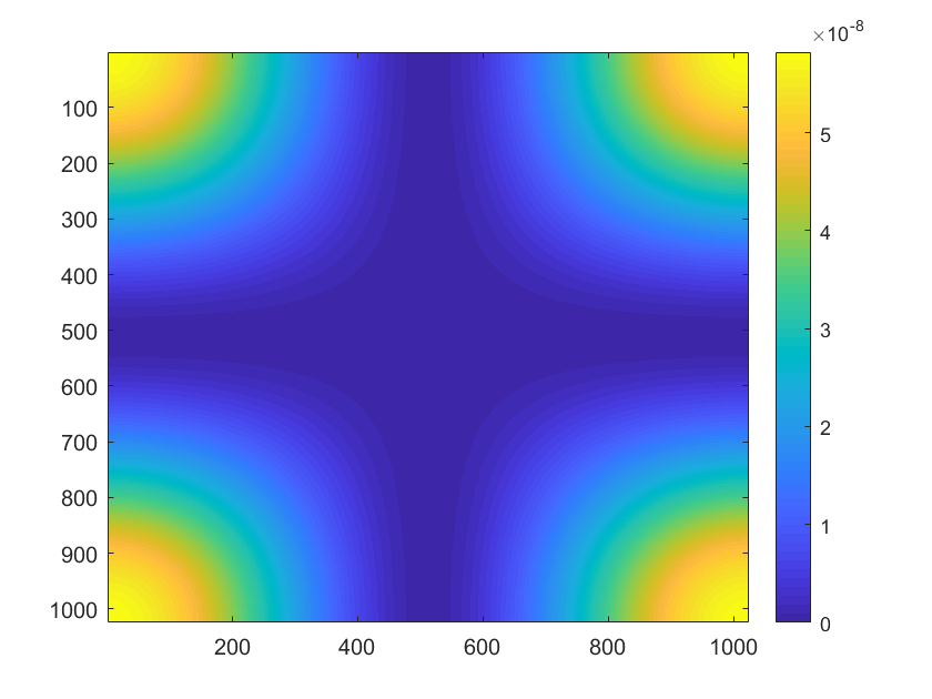
(a)

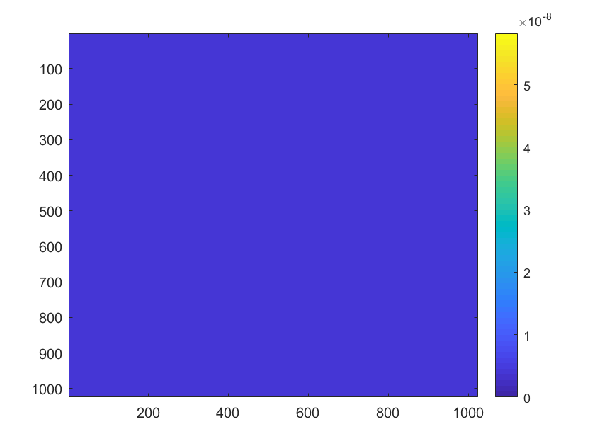
(b)

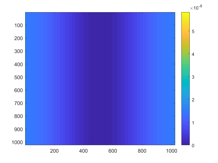
(c)

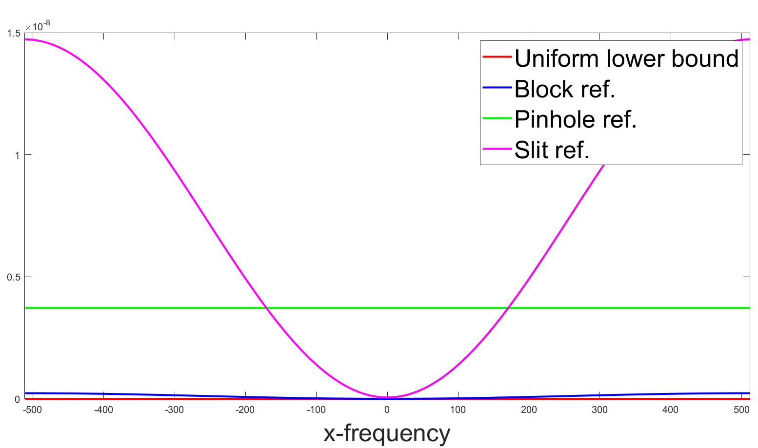
(d)

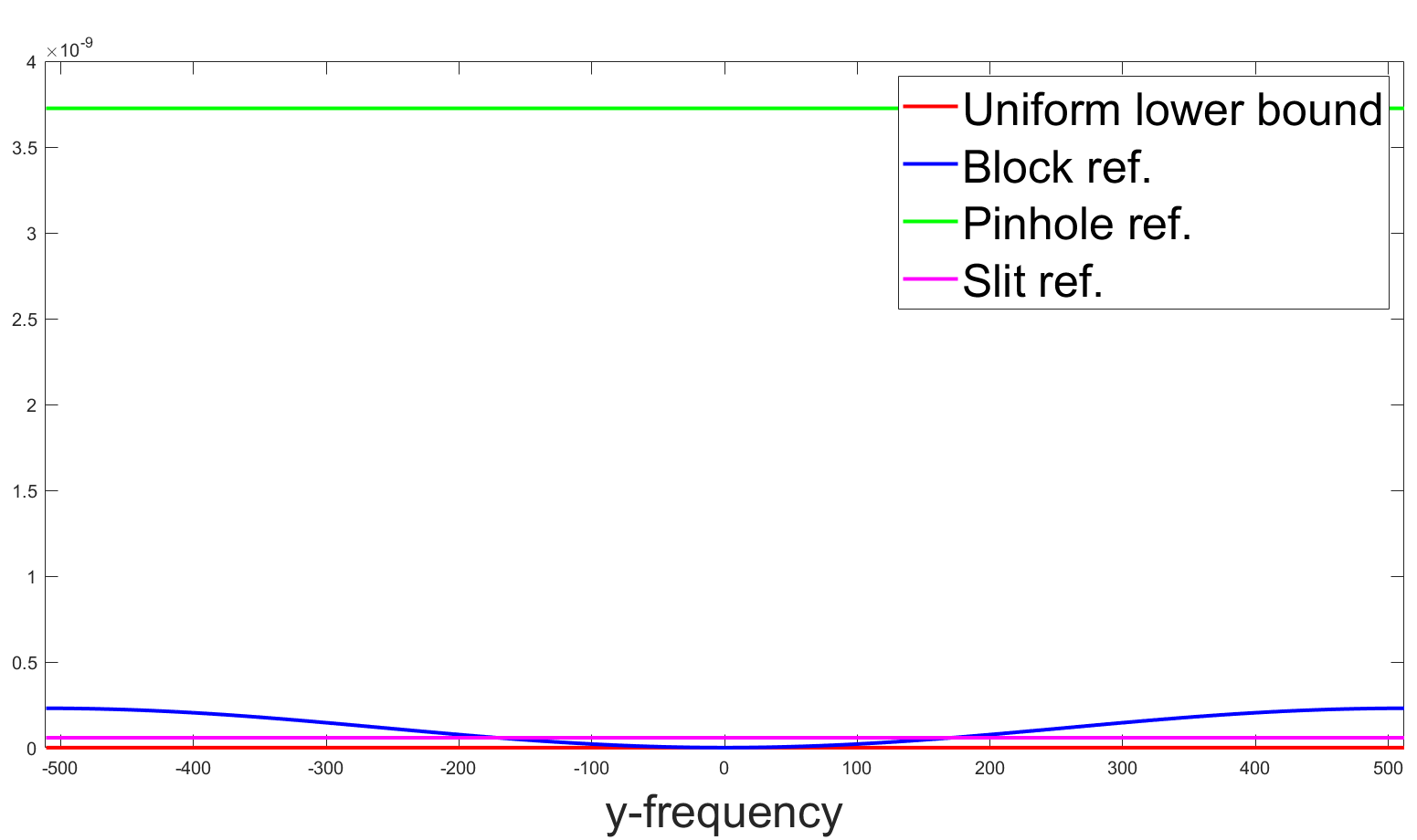
(e)

Figure 7: Plot of $S_{R}$ for the three special references and the uniform lower bound established in Theorem 3.5. Fig. 7(a),Fig. 7(b),Fig. 7(c) show the $S_{R}$ for the block, pinhole, and slit references, respectively. Fig. 7(d) and Fig. 7(e) show the cross-sections cutting the origin and parallel to the $x$ and $y$ directions, respectively. While the pinhole reference induces a flat scaling to the entire spectrum (as predicted in Theorem 3.7), the values for the block references are small at the low frequencies, and grow toward larger values moving into high frequencies. The slit reference interpolates the behaviors across directions: along the $y$-axis, the values are constant—same as the pinhole reference, but along the $x$-axis, the value increases as the frequency grows, similarly to the block reference.

Note that these observations describe how the reference scaling factor $S_{R}$ depends on the reference choice $R$. This only partially describes the effect of the reference choice $R$ on the expected error given in Eq. 3.4. Of course, the choice of $R$ will also affect $Y$ itself. However, the effect of $R$ on the former will typically far outweigh the latter by several orders of magnitude. We provide a sketch argument explaining this below.

In Eq. 3.4, both $Y=|\widehat{[X,R]}|^{2}$ and $S_{R}$ depend on the reference $R$, and both $Y$ and $S_{R}$ contribute to the expected error.

• For $Y$, note that

  $$|\widehat{[X,R]}|^{2} =|\widehat{[X,0]}+\widehat{[0,R]}|^{2}\quad\text{(Fourier transform is a linear operator)}$$ (3.10)

  $$=|\widehat{[X,0]}|^{2}+|\widehat{[0,R]}|^{2}+2\Re\left(\widehat{[X,0]}\odot\widehat{[0,R]}\right),$$ (3.11)

  where $\odot$ denotes the elementwise Hadamard product. Moreover,

  $$\left\|Y\right\|_{1}=\|\widehat{[X,R]}\|_{F}^{2}=m^{2}\|[X,R]\|_{F}^{2}=m^{2}\left\|X\right\|_{F}^{2}+m^{2}\left\|R\right\|_{F}^{2},$$ (3.12)

  where the second equality follows from Parseval’s theorem.

• The $S_{R}$ term changes significantly across the references: for example, on a $64\times 64$ image, the zero-frequency scaling term $S_{R}(0,0)$ for the block reference is $1/64$ of that for the slit reference, and is $1/64^{2}$ of that for the pinhole reference, as implied by Theorems 3.7, 3.8 and 3.9. By Theorem 3.7, the pinhole reference induces a “flat” weighting scheme with a uniform weight $n^{2}/m^{4}$. By contrast, the weights induced by the block reference are frequency-varying (Theorem 3.9): when one of $k_{1}$ and $k_{2}$ is reasonably small, the weights are on the order $O(n/m^{4})$, and when both are small, the weights are on the optimal order $O(1/m^{4})$, which matches the lower bound given by Theorem 3.5. The weights induced by the slit reference interpolate the previous two in different directions: for a fixed $k_{2}$, the weight is constant and the behavior matches that of the pinhole reference, whereas the behavior is similar to that of the block reference when $k_{2}$ changes. The weighting behaviors of the three references are demonstrated in Fig. 7.

To illustrate how Eq. 3.4 and the above facts can help provide insights into reference design and choice, we look at two stylized cases. For this discussion, reference choice is confined to the three special references we discussed above.

• Case I: Spectrum of $X$ concentrates on (super) low-frequency bands. A good example is when $X=\mathbf{1}_{n\times n}$. We think of $X$ as “flat” and has values on the order of $\Theta(1)$. So $\left\|X\right\|_{F}^{2}\in\Theta(n^{2})$. Then whatever the choice of $R$, $\left\|X\right\|_{F}^{2}+\left\|R\right\|_{F}^{2}\in\Theta(n^{2})$. So the contribution by $\left\|Y\right\|_{1}$ only differs across the three references by a small constant factor. Moreover, by Eq. 3.10, $Y$ is low-frequency dominant regardless of the reference. According to our above discussion about the weight distribution of $S_{R}$, using the block reference might be beneficial for this class of signals (depending on of course how concentrated the low-frequency components of $Y$ is).

• Case II: Spectrum of $X$ is flat or has significant medium- to high-frequency components. An idealized example is when $X=\delta(0,0)$, and we focus on the pinhole and block references. For either of them, the medium- to high-frequency components in $S_{R}$ are on the same order (i.e., $O(n^{2}/m^{4})$ from Theorem 3.7 and Theorem 3.9), and in $Y$ are on the same order also (i.e., $O(1)$). For the low-frequency part, $S_{R_{b}}$ are $O(1/m^{4})$, and $S_{R_{p}}$ are $O(n^{2}/m^{4})$. Moreover, for the low-frequency part of $Y$, $|\widehat{[X,R_{b}]}|^{2}$ are dominated by $|\widehat{[0,R_{b}]}|^{2}$, which is $O(n^{2})$, and $|\widehat{[X,R_{p}]}|^{2}$ are $O(1)$. Thus, $\left\langle S_{R},Y\right\rangle$ are on the same order whether we choose the block or the pinhole reference. So the final performance of the two is largely determined by $\left\|Y\right\|_{1}$. When $\left\|X\right\|_{F}\in o(n^{2})$, say $\left\|X\right\|_{F}=1$ (for $\delta(0,0)$), obviously the pinhole reference is more favorable, as $\left\|R_{p}\right\|_{F}^{2}=1$ whereas $\left\|R_{b}\right\|_{F}^{2}=n^{2}$. But if $\left\|X\right\|_{F}^{2}\in\Theta(n^{2})$, we do not expect substantial differences.

It is natural to expect a smooth transition of the behaviors moving from the super-flat signal $\mathbf{1}_{n\times n}$ to the super sharp $\delta(0,0)$. We confirm the differential behaviors of the references empirically in Section 4.

3.4 Error Perturbation

Our error formula Eq. 3.4 gives only the expected squared recovery error, and our results in Section 3.2 and particularly the optimality analysis in Section 3.3 are derived based on this expected error. One may wonder if it is reasonable to base the analysis solely on expectation. The following perturbation bound provides some insights in this direction.

Theorem 3.10.

For each of the pinhole, slit, and block references, and for the Poisson noise model on $\widetilde{Y}$ given by Eq. 3.3, the following holds. For all $t>0$,

$$\mathbb{P}\left[\left|\left\|\widetilde{X}-X\right\|_{F}^{2}-\mathbb{E}\left\|\widetilde{X}-X\right\|_{F}^{2}\right|\geq t\right]\\ \leq 2\exp\left\{-c\min\left(\frac{N_{p}mt^{1/2}}{\sqrt{3N_{p}\left\|Y\right\|_{1}\left\|Y\right\|_{\infty}}+2\left\|Y\right\|_{1}},\frac{N_{p}^{4}m^{4}t^{2}}{n^{2}\left(\sqrt{3N_{p}\left\|Y\right\|_{1}\left\|Y\right\|_{\infty}}+2\left\|Y\right\|_{1}\right)^{4}}\right)\right\},$$ (3.13)

where $c>0$ is a universal constant.

Proof of this theorem is included in Appendix B. To make sense of this theorem, let us plug in some practical values for the parameters: $t=n^{2}t_{0}$ (i.e., $t_{0}$ is the average pixel-wise perturbation), $N_{p}=C_{0}m^{2}$ for a large constant $C_{0}$, $\left\|Y\right\|_{1}$ is typically $O(m^{2}n^{2})$ and $\left\|Y\right\|_{\infty}$ is typically $O(n^{2})$ (i.e., the spectrum is not too peaky). Then we have

$$\frac{N_{p}mt^{1/2}}{\sqrt{3N_{p}\left\|Y\right\|_{1}\left\|Y\right\|_{\infty}}+2\left\|Y\right\|_{1}} =c_{1}C_{0}\frac{m}{n}t_{0}^{1/2},$$ (3.14)

$$\frac{N_{p}^{4}m^{4}t^{2}}{n^{2}\left(\sqrt{3N_{p}\left\|Y\right\|_{1}\left\|Y\right\|_{\infty}}+2\left\|Y\right\|_{1}\right)^{4}} =c_{2}C_{0}^{4}\frac{m^{4}}{n^{6}}t_{0}^{2}.$$ (3.15)

Evidently, making $C_{0}$ large and $m$ large (relative to $n$) improves the concentration. For example, in our experiment below, $C_{0}\gg 100>n$ and $m\geq 10n$, making the above exponents reasonably large and hence the tail probability negligibly small even for small $t_{0}$.

4 Numerical Simulations

We perform numerical experiments on two sets of data to illustrate the effectiveness of the referenced deconvolution algorithm (Section 2.3), and to corroborate the theoretical prediction on optimal reference design (Section 3.3). Codes for these experiments are available at https://github.com/sunju/REF_CDI.

4.1 On the Mimivirus Image

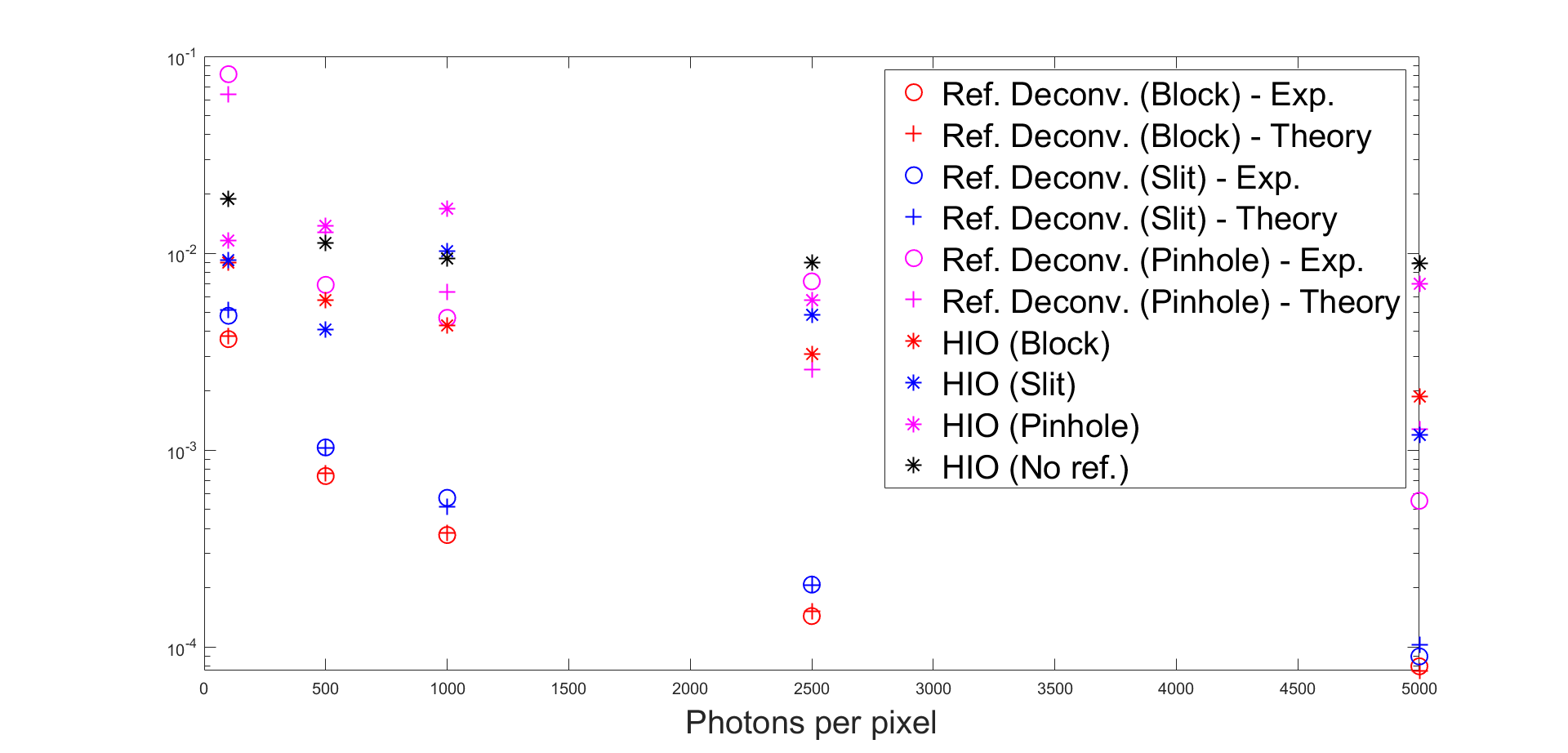
Figure 8: Plot of the relative recovery error against the nominal photon level for experiments on the mimivirus image. Result from both the referenced deconvolution and the classic HIO algorithms are included. For the referenced deconvolution algorithm, both the expected and empirical recovery errors are presented. The referenced deconvolution algorithm combined with the block reference performs consistently better than other algorithm-reference combinations. Also, for each reference, the expected recovery error closely matches the empirical recovery error, as predicted by Theorem 3.10.

(a) Ground-truth
image

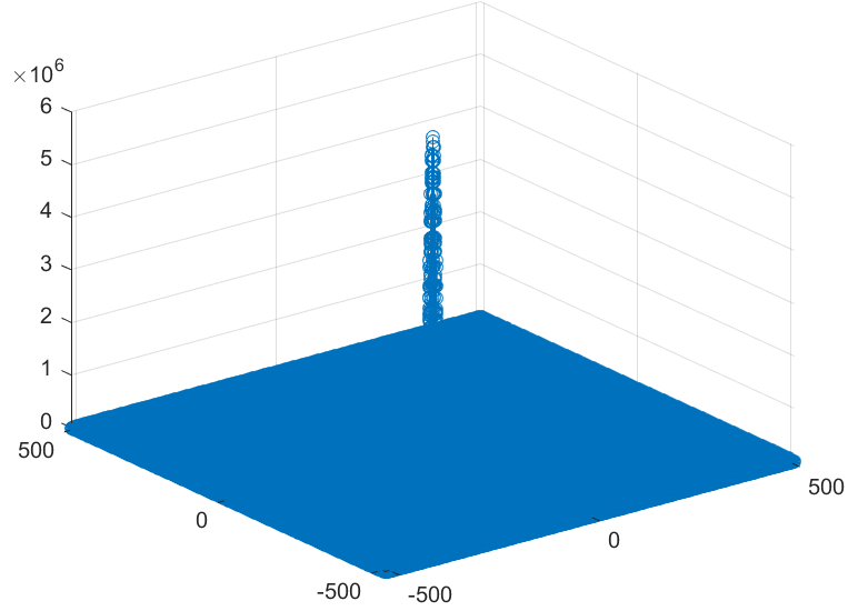
(b) Fourier magnitude
of the groundtruth

(c) HIO (no ref.)
$\varepsilon=93.794$, $\mathbb{E}\left[\varepsilon\right]$ NA

(d) Ref. Deconv. with block ref.
$\varepsilon=3.7029$, $\mathbb{E}\left[\varepsilon\right]=3.7953$

(e) Ref. Deconv. with slit ref.
$\varepsilon=5.7200$, $\mathbb{E}\left[\varepsilon\right]=5.1467$

(f) Ref. Deconv. with pinhole ref.
$\varepsilon=46.966$, $\mathbb{E}\left[\varepsilon\right]=63.835$

(g) HIO with block ref.
$\varepsilon=42.813$, $\mathbb{E}\left[\varepsilon\right]$ NA

(h) HIO with slit ref.
$\varepsilon=102.28$, $\mathbb{E}\left[\varepsilon\right]$ NA

(i) HIO with pinhole ref.
$\varepsilon=168.18$, $\mathbb{E}\left[\varepsilon\right]$ NA

Figure 9: Recovery result of the mimivirus image using various recovery schemes, and the corresponding relative recovery errors (all errors should be rescaled by $10^{-4}$). The photon level is fixed at $N_{pp}=1000$. Referenced deconvolution achieves superior recovery to HIO, both with and without the reference information enforced. Experimental and theoretical relative errors for referenced deconvolution closely match, as predicted by Theorem 3.10. The block reference achieves the best recovery.

In this experiment, the specimen $X$ is the mimivirus image [GKL⁺08], and its spectrum mostly concentrates on very low frequencies, as shown in Fig. 10(b). The image size is $64\times 64$, and the pixel values are normalized to $[0,1]$. For the referenced setup, a reference $R$ of size $64\times 64$ is placed next to $X$, forming a composite specimen $[X,R]$ of size $64\times 128$. Three references, i.e., the pinhole, the slit, and the block references are considered. The oversampled Fourier transform is taken to be of size $1024\times 1024$, and the collected noisy data $\widehat{Y}$ obeys the Poisson shot noise model defined in Eq. 3.3. For this model, the nominal number of total photons $N_{p}$ is given by $N_{pp}\times 1024^{2}$, where $N_{pp}$ can be understood to be the average number of photons to be received by each pixel. We investigate the regime where $N_{pp}$ varies from $100$ to $5000$ ($N_{pp}=100,500,1000,2500,5000$, respectively), with one simulation trial run for each $N_{pp}$ value.

We run the referenced deconvolution algorithm and also the classic HIO algorithm with and without enforcing the known reference for comparison. The results are presented in Fig. 8 and Fig. 9. We define the relative (squared) recovery error to be

$$\varepsilon\doteq\frac{\left\|X-\widehat{X}\right\|^{2}}{\left\|X\right\|^{2}}.$$ (4.1)

From Fig. 8, it is evident that for the referenced deconvolution schemes, the expected and empirical relative recovery errors are close (justified by the perturbation result in Section 3.4). Moreover, referenced deconvolution combined with the block reference performs the best among all the algorithm and reference combinations—regardless of the photon per pixel level $N_{pp}$. The superiority of the block reference among the referenced deconvolution schemes agrees with the prediction in Section 3.3, as the spectrum of $X$ sharply concentrates on very low frequencies. In addition, for the referenced deconvolution schemes, the recovery errors generally decrease as the photon level (dictated by $N_{pp}$) increases. This trend is clearly predicted by Eq. 3.4: because only $N_{p}=N_{pp}\times 1024^{2}$ depends on $N_{pp}$, the expected squared error is proportional to $1/N_{pp}$. The relative errors and recovered images for $N_{pp}=1000$ are exhibited in Fig. 9.

In regards to algorithm runtime for our experiments, the referenced deconvolution algorithm runs in less than 0.001 seconds for all three reference choices considered. The runtime for HIO is about 0.2 seconds per iteration, with the iteration with the smallest relative error selected from 1000 iterations.

4.2 On a “Flat-Spectrum” Image

(a) Ground-truth
image

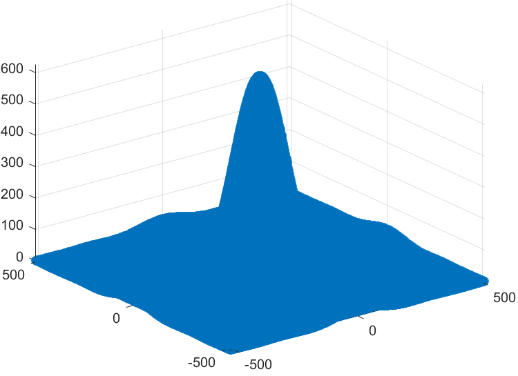
(b) Fourier magnitude
of the groundtruth

(c) HIO (no ref.)
$\varepsilon=21577$, $\mathbb{E}\left[\varepsilon\right]$ NA

(d) Ref. Deconv. with block ref.
$\varepsilon=91.203$, $\mathbb{E}\left[\varepsilon\right]=83.723$

(e) Ref. Deconv. with slit ref.
$\varepsilon=1.8769$, $\mathbb{E}\left[\varepsilon\right]=1.8496$

(f) Ref. Deconv. with pinhole ref.
$\varepsilon=1.0609$, $\mathbb{E}\left[\varepsilon\right]=1.0609$

(g) HIO with block ref.
$\varepsilon=760.10$, $\mathbb{E}\left[\varepsilon\right]$ NA

(h) HIO with slit ref.
$\varepsilon=1453.1$, $\mathbb{E}\left[\varepsilon\right]$ NA

(i) HIO with pinhole ref.
$\varepsilon=12855$, $\mathbb{E}\left[\varepsilon\right]$ NA

Figure 10: Recovery result of the “centered square” image using various recovery schemes, and the corresponding relative recovery errors (all errors should be rescaled by $10^{-4}$). The photon level $N_{pp}$ is fixed as $1000$. Referenced deconvolution achieves superior recovery to HIO (with the reference information enforced). Experimental and theoretical relative errors for referenced deconvolution closely match, as predicted by Theorem 3.10. The pinhole reference achieves the best recovery.

In this experiment, the image contains a small centered square. Except for this, the basic experimental setup is identical to the above one. We focus on the case $N_{pp}=1000$. In terms of recovery error, the referenced deconvolution schemes perform uniformly better than the HIO schemes, just as for the mimivirus image. For the current “centered square” image which has a considerably “flat” spectrum (see Fig. 10(b)), however, the best-performing reference is the pinhole reference—again consistent with our theoretical prediction in Section 3.3. The detailed recovery results and recovery errors are presented in Fig. 10.

5 Discussion

We have presented a general mathematical framework for the holographic phase retrieval problem, and proposed the referenced deconvolution algorithm as a generic solution scheme. Our formulation emphasizes the structure in the linear deconvolution procedure, and offers new insights into the resulting linear systems from popular reference choices.

We have also derived a general formula for the expected recovery error of the referenced deconvolution algorithm when the measurement data contains stochastic noise. Under a Poisson shot noise model, the formula allows us to compare popular reference choices and conclude that the block reference minimizes low-frequency contributions to the recovery error and is hence favorable for typical imaging data.

Building on our framework, it is possible to perform more detailed analysis of other noise models and reference choices. Also, the insights obtained here can likely motivate further design possibilities. In our follow-up work [BSC⁺19], one such new reference setup (termed the dual-reference) is proposed, which provides superior noise stability across the frequency spectrum, as compared to popular single-reference setups.

Another possible extension is to include beamstops, which are often implemented in practical CDI experiments [GSF07, HSC15]. Beamstops effectively remove a small fraction ($\leq 5\%$) of low-frequency components from the measurements. We observe that the proposed referenced deconvolution algorithm is easily adapted to this setting, insofar as the missing data does not render the problem ill-conditioned.

6 Acknowledgments

The authors are grateful to the Simons Foundation Math+X initiative and the Natural Science and Engineering Research Council of Canada for providing support during our study. We would also like to sincerely thank Walter Murray, Gordon Wetzstein, and Jon Claerbout for ongoing valuable feedback towards developing this work.

Appendix A Connection with HERALDO

We sketch the correspondence between the Referenced Deconvolution algorithm and the HERALDO procedure [GSF07].

A.1 Summary of HERALDO

The HERALDO procedure (an acronym for “Holography with Extended Reference by Autocorrelation Linear Differential Operation”) considers a continuous setup with a specimen $X(x,y)$ and reference $R(x,y)$ which together form the composite $F(x,y)=X(x,y)+R(x,y)$. Let $\star$ denote the cross-correlation. It follows that

$$F\star F=X\star X+R\star R+X\star R+R\star X.$$ (A.1)

Provided that $R$ and $X$ satisfy certain separation conditions, the cross-correlation $R\ast X$ will not overlap with the other terms in Eq. A.1. The HERALDO idea is to find an $n^{th}$ order weighted linear differential operator $\mathcal{L}_{R}^{n}$, i.e.,

$$\mathcal{L}^{n}_{R}=\sum_{k=0}^{n}a_{k}\frac{\partial^{n}}{\partial x^{n-k}\partial y^{k}},\quad\text{where $a_{k}$'s are the weights},$$ (A.2)

such that

$$\mathcal{L}^{n}_{R}(R)=A\delta(x-x_{0},y-y_{0})+o(x,y),$$ (A.3)

for some constants $A,x_{0},y_{0}$ and some offset function $o(x,y)$. Now, applying the key identies

$$\mathcal{L}^{(n)}\left(h\star g\right)=\mathcal{L}^{(n)}\left(h\right)\star g=\left(-1\right)^{n}h\star\mathcal{L}^{(n)}\left(g\right)\quad\forall\;h,g,$$ (A.4)

one can show that

$$\mathcal{L}^{(n)}_{R}\left(F\ast F\right)=\mathcal{L}^{(n)}_{R}\left(X\star X\right)+\frac{1}{2}\left[AR^{*}\left(x_{0}-x,y_{0}-x\right)+o\star R\right]+\left(-1\right)^{n}\frac{1}{2}\left[A^{*}R\left(x_{0}+x,y_{0}+x\right)+R\star o\right]+\\ \left(-1\right)^{n}o\star X+X\star o+\left(-1\right)^{n}A^{*}X\left(x+x_{0},y+y_{0}\right)+AX^{*}\left(x_{0}-x,y_{0}-y\right).$$

Appropriate separation conditions on the supports (i.e., domains of nonzeros) of $X$,$R$, and $o$ then ensure either $A^{*}X\left(x+x_{0},y+y_{0}\right)$ or $AX^{*}\left(x_{0}-x,y_{0}-y\right)$ be separate from other terms spatially. This provides a scaled and shifted copy of $X$, thereby recovering the unknown specimen of interest.

Note that for an arbitrary reference $R$, determining whether such an $\mathcal{L}^{n}_{R}$ exists and how it can be constructed is a highly nontrivial problem. Nonetheless, for special references such as the pinhole, slit, and block, there are easy constructions as illustrated in [GSF07].

A.2 Connection to the Referenced Deconvolution Algorithm

The HERALDO procedure seeks a continuous linear differential operator $\mathcal{L}^{n}_{R}$ such that $\mathcal{L}^{n}_{R}(R)=A\delta(x-x_{0},y-y_{0})+o(x,y)$. Consider the special case where $A=1$, $x_{0}=y_{0}=0$, and $o(x,y)=0$, whence

$$\mathcal{L}^{n}_{R}(R)=\delta(x,y).$$ (A.5)

The paper [GSF07] has derived the respective linear differential operators with $n\leq 2$ for the pinhole, slit, and block references. For each of these three special references, we observe that $M_{R}^{-1}$ is exactly a finite-difference approximation to the linear differential operator derived in [GSF07], which is elaborated below.

A.2.1 Pinhole Reference

For the pinhole reference $R_{p}$, $\mathcal{L}^{n}_{R_{p}}$ is simply the identity operator, and hence its discretized version is simply the identity matrix, as is $M_{R_{p}}^{-1}$.

A.2.2 Slit Reference

For the slit reference $R_{s}$, $\mathcal{L}^{n}_{R_{s}}$ is shown in Section 4.1 of [GSF07] to be $\frac{\partial}{\partial y}$, i.e., vertical first-order differential operator, which can be approximated by $M_{R_{s}}^{-1}=I\otimes D_{n}$ (see Eq. 2.19), as $\left(I\otimes D_{n}\right)\operatorname{vec}\left(R_{s}\right)=\operatorname{vec}\left(D_{n}R_{s}I\right)$. Here $D_{n}$ is the first-order difference matrix that performs finite differencing vertically.

A.2.3 Block Reference

For the slit reference $R_{b}$, $\mathcal{L}^{n}_{R_{b}}$ is shown in Section 4.3 of [GSF07] to be $\frac{\partial^{2}}{\partial x\partial y}$, which can be approximated by $M_{R_{b}}^{-1}=D_{n}\otimes D_{n}$ (see Eq. 2.23), as $\left(D_{n}\otimes D_{n}\right)\operatorname{vec}\left(R_{b}\right)=\operatorname{vec}\left(D_{n}R_{b}D_{n}^{\top}\right)$.

Overall, the referenced deconvolution method can be easily applied to any arbitrary reference $R$. In contrast, the HERALDO procedure can only be applied when $\mathcal{L}^{n}_{R}$ exists and can be constructed, which has to date only been demonstrated for special references with simple geometric shapes—so that the specific construction of $\mathcal{L}^{n}_{R}$ is straightforward. However, it may not be easily applicable to reference choices such as the annulus [GO18] or uniformly redundant array [MBS⁺08].

Appendix B Proof of Theorem 3.10

Let $\eta\doteq\left\|\widetilde{X}-X\right\|_{F}^{2}$. We are interested to control $\left|\eta-\mathbb{E}\eta\right|$. By similar manipulation as in Lemma 3.3, we have

$$\left\|\widetilde{X}-X\right\|_{F}^{2}-\mathbb{E}\left\|\widetilde{X}-X\right\|_{F}^{2}\\ =\left\langle T_{R}^{*}T_{R},\left[\operatorname{vec}\left(\widetilde{Y}\right)-\operatorname{vec}\left(Y\right)\right]\left[\operatorname{vec}\left(\widetilde{Y}\right)-\operatorname{vec}\left(Y\right)\right]^{*}-\mathbb{E}\left[\operatorname{vec}\left(\widetilde{Y}\right)-\operatorname{vec}\left(Y\right)\right]\left[\operatorname{vec}\left(\widetilde{Y}\right)-\operatorname{vec}\left(Y\right)\right]^{*}\right\rangle.$$

Since entries in $\operatorname{vec}(\widetilde{Y})-\operatorname{vec}(Y)$ have sub-exponential tails, we need Hanson-Wright type inequalities for sub-exponential random variables.

Theorem B.1 (Proposition 1.1 of [GSS19]).

Let $A\in\mathbb{R}^{n\times n}$ be a symmetric matrix and let $Z_{1},\dots,Z_{n}$ be a set of independent random variables with $\mathbb{E}Z_{i}=0$ and $\left\|Z_{i}\right\|_{\psi_{1}}\leq M$ for all $i$ (here $\left\|\cdot\right\|_{\psi_{1}}$ is the sub-exponential norm as defined in, e.g., Definition 2.7.5. of [Ver18]). Write $Z\doteq[Z_{1};\dots;Z_{n}]$ . For any $t>0$,

$$\mathbb{P}\left[\left|Z^{\top}AZ-\mathbb{E}Z^{\top}AZ\right|\geq t\right]\leq 2\exp\left(-c\min\left\{\frac{t^{2}}{M^{4}\left\|A\right\|_{F}^{2}},\frac{t^{1/2}}{M\left\|A\right\|^{1/2}}\right\}\right).$$ (B.1)

Note that

$$\left\langle T_{R}^{*}T_{R},\left[\operatorname{vec}\left(\widetilde{Y}\right)-\operatorname{vec}\left(Y\right)\right]\left[\operatorname{vec}\left(\widetilde{Y}\right)-\operatorname{vec}\left(Y\right)\right]^{*}\right\rangle=\left[\operatorname{vec}\left(\widetilde{Y}\right)-\operatorname{vec}\left(Y\right)\right]^{*}\left(T_{R}^{*}T_{R}\right)\left[\operatorname{vec}\left(\widetilde{Y}\right)-\operatorname{vec}\left(Y\right)\right].$$

So, in our problem, the random vector $Z$ is $\operatorname{vec}\left(\widetilde{Y}\right)-\operatorname{vec}\left(Y\right)$

$$Z_{k}\doteq\widetilde{Y}_{ij}-Y_{ij}.$$ (B.2)

By our Poisson model,

$$\mathbb{E}\left[\widetilde{Y}_{ij}-Y_{ij}\right]=Y_{ij}-Y_{ij}=0.$$ (B.3)

Now we need to estimate the sub-exponential norm of a centered Poisson random variable.

Lemma B.2.

Let $Z\sim\mathrm{Pois}\left(\lambda\right)$. We have

$$\left\|Z-\lambda\right\|_{\psi_{1}}\leq C\left(\sqrt{3\lambda}+2\right),$$ (B.4)

where $C>0$ is a universal constant.

Proof. Applying the Cramer-Chernoff method to $Z-\lambda$, we obtain that (see, e.g., Page 23 of [BLM13])

$$\mathbb{P}\left[Z-\lambda>t\right] \leq\exp\left\{-\lambda h\left(t/\lambda\right)\right\} \quad\forall\;t\geq 0,$$ (B.5)

$$\mathbb{P}\left[Z-\lambda<-t\right] \leq\exp\left\{-\lambda h\left(-t/\lambda\right)\right\} \quad\forall\;t\in[0,\lambda],$$ (B.6)

where $h(u)\doteq\left(1+u\right)\log(1+u)-u$. Using that $h(u)\geq\frac{u^{2}}{2\left(1+u/3\right)}$, we can write the above results collectively as

$$\mathbb{P}\left[\left|Z-\lambda\right|>t\right]\leq 2\exp\left(-\frac{t^{2}}{2\lambda+2t/3}\right)\quad\forall\;t>0.$$ (B.7)

Now we will estimate the sub-exponential norm by upper bounding the moments $\mathbb{E}\left|Z-\lambda\right|^{p}$. We have

$$\mathbb{E}\left|Z-\lambda\right|^{p}=\; \int_{0}^{\infty}\mathbb{P}\left[\left|Z-\lambda\right|^{p}\geq u\right]\;du$$ (B.8)

$$=\; \int_{0}^{\infty}\mathbb{P}\left[\left|Z-\lambda\right|\geq t\right]pt^{p-1}\;dt$$ (B.9)

$$\leq\; 2p\int_{0}^{\infty}\exp\left(-\frac{t^{2}}{2\lambda+2t/3}\right)t^{p-1}\;dt$$ (B.10)

$$=\; 2p\int_{0}^{\frac{3}{2}\lambda}\exp\left(-\frac{t^{2}}{2\lambda+2t/3}\right)t^{p-1}\;dt+2p\int_{\frac{3}{2}\lambda}^{\infty}\exp\left(-\frac{t^{2}}{2\lambda+2t/3}\right)t^{p-1}\;dt$$ (B.11)

$$\leq\; 2p\int_{0}^{\frac{3}{2}\lambda}\exp\left(-\frac{t^{2}}{3\lambda}\right)t^{p-1}\;dt+2p\int_{\frac{3}{2}\lambda}^{\infty}\exp\left(-\frac{t}{2}\right)t^{p-1}\;dt\;$$ (B.12)

$$\leq\; 2p\int_{0}^{\infty}\exp\left(-\frac{t^{2}}{3\lambda}\right)t^{p-1}\;dt+2p\int_{0}^{\infty}\exp\left(-\frac{t}{2}\right)t^{p-1}\;dt$$ (B.13)

$$\leq\; \left(3\lambda\right)^{p/2}p\Gamma\left(p/2\right)+2^{p+1}p\Gamma(p)\leq\left(3\lambda\right)^{p/2}p\left(p/2\right)^{p/2}+2^{p+1}p^{p+1},$$ (B.14)

where we used $\Gamma(x)\leq x^{x}$ to obtain the very last bound. Thus,

$$\left\|Z-\lambda\right\|_{L_{p}}=\left(\mathbb{E}\left|Z-\lambda\right|^{p}\right)^{1/p}\leq 5\left(\sqrt{3\lambda}+2\right)p.$$ (B.15)

We obtain the claimed result by connecting the above moment bound with the definition of sub-exponential norm, see, e.g., Proposition 2.7.1 of [Ver18]. ∎

We are ready now to state the concentration of the empirical (squared) error around the expectation.

Theorem B.3.

For any of the three special (i.e., pinhole, slit, block) references, the following holds: for all $t>0$,

$$\mathbb{P}\left[\left|\left\|\widetilde{X}-X\right\|_{F}^{2}-\mathbb{E}\left\|\widetilde{X}-X\right\|_{F}^{2}\right|\geq t\right]\\ \leq 2\exp\left(-c\min\left\{\frac{N_{p}mt^{1/2}}{\sqrt{3N_{p}\left\|Y\right\|_{1}\left\|Y\right\|_{\infty}}+2\left\|Y\right\|_{1}},\frac{N_{p}^{4}m^{4}t^{2}}{n^{2}\left(\sqrt{3N_{p}\left\|Y\right\|_{1}\left\|Y\right\|_{\infty}}+2\left\|Y\right\|_{1}\right)^{4}}\right\}\right).$$ (B.16)

Here $c>0$ is a universal constant.

Proof. By our Poisson noise model and Lemma B.2 ,

$$\left\|Y_{ij}-\widetilde{Y}_{ij}\right\|_{\psi_{1}}\leq C\frac{\left\|Y\right\|_{1}}{N_{p}}\left(\sqrt{\frac{3N_{p}}{\left\|Y\right\|_{1}}Y_{ij}}+2\right).$$ (B.17)

So in applying Theorem B.1, we can take $M=C\frac{\left\|Y\right\|_{1}}{N_{p}}\left(\sqrt{\frac{3N_{p}}{\left\|Y\right\|_{1}}\left\|Y\right\|_{\infty}}+2\right)$.

Now we estimate $\left\|T_{R}^{*}T_{R}\right\|=\left\|T_{R}\right\|^{2}$, and $\left\|T_{R}^{*}T_{R}\right\|_{F}$. Note the fact that for any two matrices $A,B$, $\left\|A\otimes B\right\|=\left\|A\right\|\left\|B\right\|$, $\left\|A\otimes B\right\|_{F}=\left\|A\right\|_{F}\left\|B\right\|_{F}$, and $\left\|AB\right\|_{F}\leq\left\|A\right\|\left\|B\right\|_{F}$. First, we have the following estimates

$$\left\|\left(P_{2}F_{RA}^{*}\right)\otimes\left(P_{1}F_{LA}^{*}\right)\right\|=\left\|P_{2}F_{RA}^{*}\right\|\left\|P_{1}F_{LA}^{*}\right\|=\sqrt{m}\times\sqrt{m}=m,$$ (B.18)

and

$$\left\|\left[\left(P_{2}F_{RA}^{*}\right)\otimes\left(P_{1}F_{LA}^{*}\right)\right]^{*}\left[\left(P_{2}F_{RA}^{*}\right)\otimes\left(P_{1}F_{LA}^{*}\right)\right]\right\|_{F} =\left\|\left[\left(P_{2}F_{RA}^{*}\right)\otimes\left(P_{1}F_{LA}^{*}\right)\right]\left[\left(P_{2}F_{RA}^{*}\right)\otimes\left(P_{1}F_{LA}^{*}\right)\right]^{*}\right\|_{F}$$

$$=\left\|\left[\left(P_{2}F_{RA}^{*}\right)\otimes\left(P_{1}F_{LA}^{*}\right)\right]\left[\left(F_{RA}P_{2}^{*}\right)\otimes\left(F_{LA}P_{1}^{*}\right)\right]\right\|_{F}$$

$$=\left\|\left(P_{2}F_{RA}^{*}F_{RA}P_{2}^{*}\right)\otimes\left(P_{1}F_{LA}^{*}F_{LA}P_{1}^{*}\right)\right\|_{F}$$

$$=m^{2}\left\|P_{2}P_{2}^{*}\right\|_{F}\left\|P_{1}P_{1}^{*}\right\|_{F}=m^{2}n.$$ (B.19)

So specializing to the references, we have

• For the pinhole reference,

  $$\left\|T_{R_{p}}\right\| =\frac{1}{m^{2}}\left\|\left(P_{2}F_{RA}^{*}\right)\otimes\left(P_{1}F_{LA}^{*}\right)\right\|=\frac{1}{m},$$ (B.20)

  $$\left\|T_{R_{p}}^{*}T_{R_{p}}\right\|_{F} \leq\frac{1}{m^{4}}\left\|\left[\left(P_{2}F_{RA}^{*}\right)\otimes\left(P_{1}F_{LA}^{*}\right)\right]^{*}\left[\left(P_{2}F_{RA}^{*}\right)\otimes\left(P_{1}F_{LA}^{*}\right)\right]\right\|_{F}=\frac{m^{2}n}{m^{4}}=\frac{n}{m^{2}}.$$ (B.21)

• For the slit reference,

  $$\left\|T_{R_{s}}\right\|\leq\frac{1}{m^{2}}\left\|D_{n}\right\|\left\|\left(P_{2}F_{RA}^{*}\right)\otimes\left(P_{1}F_{LA}^{*}\right)\right\|\leq\frac{2}{m},$$ (B.22)

  where we used $\left\|D_{n}\right\|\leq 2$. Moreover,

  $$\left\|T_{R_{s}}^{*}T_{R_{s}}\right\|_{F}\leq\frac{1}{m^{4}}\left\|D_{n}\right\|^{4}\left\|\left[\left(P_{2}F_{RA}^{*}\right)\otimes\left(P_{1}F_{LA}^{*}\right)\right]^{*}\left[\left(P_{2}F_{RA}^{*}\right)\otimes\left(P_{1}F_{LA}^{*}\right)\right]\right\|_{F}\leq\frac{4n}{m^{2}}.$$ (B.23)

• For the block reference,

  $$\left\|T_{R_{b}}\right\| \leq\frac{1}{m^{2}}\left\|D_{n}\right\|^{2}\left\|\left(P_{2}F_{RA}^{*}\right)\otimes\left(P_{1}F_{LA}^{*}\right)\right\|\leq\frac{4}{m},$$ (B.24)

  $$\left\|T_{R_{b}}^{*}T_{R_{b}}\right\|_{F} \leq\frac{1}{m^{4}}\left\|D_{n}\right\|^{2}\left\|\left[\left(P_{2}F_{RA}^{*}\right)\otimes\left(P_{1}F_{LA}^{*}\right)\right]^{*}\left[\left(P_{2}F_{RA}^{*}\right)\otimes\left(P_{1}F_{LA}^{*}\right)\right]\right\|_{F}\leq\frac{16n}{m^{2}}.$$ (B.25)

So for all the three references, we have

$$\left\|T_{R}^{*}T_{R}\right\|\leq\frac{16}{m^{2}},\quad\left\|T_{R}^{*}T_{R}\right\|_{F}\leq\frac{16n}{m^{2}}.$$ (B.26)

Substituting the estimates into Theorem B.1, we obtain the claimed result. ∎

References

- [BBE17] Tamir Bendory, Robert Beinert, and Yonina C. Eldar, Fourier phase retrieval: Uniqueness and algorithms, Springer International Publishing, Cham, 2017.
- [BDP+07] Oliver Bunk, Ana Diaz, Franz Pfeiffer, Christian David, Bernd Schmitt, Dillip K Satapathy, and J Friso van der Veen, Diffractive imaging for periodic samples: retrieving one-dimensional concentration profiles across microfluidic channels, Acta Crystallographica Section A 63 (2007), no. 4, 306–314.
- [BLM13] Stéphane Boucheron, Gábor Lugosi, and Pascal Massart, Concentration inequalities: A nonasymptotic theory of independence, Oxford university press, 2013.
- [BPC+11] Stephen Boyd, Neal Parikh, Eric Chu, Borja Peleato, and Jonathan Eckstein, Distributed optimization and statistical learning via the alternating direction method of multipliers, Found. Trends Mach. Learn. 3 (2011), no. 1, 1–122.
- [BS17] David Barmherzig and Ju Sun, A Local Analysis of Block Coordinate Descent for Gaussian Phase Retrieval, 10th NIPS Workshop on Optimization for Machine Learning abs/1712.0 (2017).
- [BSC+19] David A. Barmherzig, Ju Sun, Emmanuel J. Candès, T. J. Lane, and Po-Nan Li, Dual-Reference Design for Holographic Coherent Diffraction Imaging, arXiv e-prints (2019), arXiv:1902.02492.
- [BSLL18] David Barmherzig, Ju Sun, Po-Nan Li, and T J Lane, On Block-Reference Coherent Diffraction Imaging, Imaging and Applied Optics 2018 (3D, AO, AIO, COSI, DH, IS, LACSEA, LS&C, MATH, pcAOP), Optical Society of America, 2018, p. CTH1B.1.
- [BTN01] A. Ben-Tal and A. Nemirovski, Lectures on modern convex optimization, Society for Industrial and Applied Mathematics, 2001.
- [CBB+06] Henry N Chapman, Anton Barty, Michael J Bogan, Sébastien Boutet, Matthias Frank, Stefan P Hau-Riege, Stefano Marchesini, Bruce W Woods, Sasa Bajt, W Henry Benner, Richard A London, Elke Plönjes, Marion Kuhlmann, Rolf Treusch, Stefan Düsterer, Thomas Tschentscher, Jochen R Schneider, Eberhard Spiller, Thomas Möller, Christoph Bostedt, Matthias Hoener, David A Shapiro, Keith O Hodgson, David van der Spoel, Florian Burmeister, Magnus Bergh, Carl Caleman, Gösta Huldt, M Marvin Seibert, Filipe R N C Maia, Richard W Lee, Abraham Szöke, Nicusor Timneanu, and Janos Hajdu, Femtosecond diffractive imaging with a soft-X-ray free-electron laser, Nature Physics 2 (2006), 839–843.
- [CESV15] E Candès, Y Eldar, T Strohmer, and V Voroninski, Phase Retrieval via Matrix Completion, SIAM Review 57 (2015), no. 2, 225–251.
- [CLS15a] E J Candès, X Li, and M Soltanolkotabi, Phase retrieval via wirtinger flow: Theory and algorithms, IEEE Trans. Inf. Theory 61 (2015), no. 4, 1985–2007.
- [CLS15b] Emmanuel J Candès, Xiaodong Li, and Mahdi Soltanolkotabi, Phase retrieval from coded diffraction patterns, Applied and Computational Harmonic Analysis 39 (2015), no. 2, 277–299.
- [DF87] J C Dainty and J R Fienup, Phase retrieval and image reconstruction for astronomy, Image Recovery: Theory and Application (H. Stark, ed.), Academic Press, 1987.
- [Els03] Veit Elser, Phase retrieval by iterated projections, J. Opt. Soc. Am. A 20 (2003), no. 1, 40–55.
- [ELS+04] S Eisebitt, J LÃŒning, W F Schlotter, M LÃtextparagraphrgen, O Hellwig, W Eberhardt, and J StÃtextparagraphhr, Lensless imaging of magnetic nanostructures by X-ray spectro-holography, Nature 432 (2004), 885–888.
- [ERT07] V Elser, I Rankenburg, and P Thibault, Searching with iterated maps, Proceedings of the National Academy of Sciences 104 (2007), no. 2, 418–423.
- [Fie78] J R Fienup, Reconstruction of an object from the modulus of its Fourier transform, Opt. Lett. 3 (1978), no. 1, 27–29.
- [Gab48] D Gabor, A New Microscopic Principle, Nature 161 (1948), 777–778.
- [GKL+08] Eric Ghigo, Jürgen Kartenbeck, Pham Lien, Lucas Pelkmans, Christian Capo, Jean-Louis Mege, and Didier Raoult, Ameobal Pathogen Mimivirus Infects Macrophages through Phagocytosis, PLOS Pathogens 4 (2008), no. 6, 1–17.
- [GO18] Tais Gorkhover and Others, Femtosecond X-ray Fourier holography imaging of free-flying nanoparticles, Nature Photonics 12 (2018), no. 3, 150–153.
- [Goo17] Joseph W. Goodman, Introduction to fourier optics, 4th ed., Macmillan Learning, New York, NY, USA, 2017.
- [GSF07] Manuel Guizar-Sicairos and James R Fienup, Holography with extended reference by autocorrelation linear differential operation, Opt. Express 15 (2007), no. 26, 17592–17612.
- [GSF08] , Direct image reconstruction from a Fourier intensity pattern using HERALDO, Opt. Lett. 33 (2008), no. 22, 2668–2670.
- [GSS19] Friedrich Götze, Holger Sambale, and Arthur Sinulis, Concentration inequalities for polynomials in -sub-exponential random variables, arXiv:1903.05964 (2019).
- [Hay82] M Hayes, The reconstruction of a multidimensional sequence from the phase or magnitude of its Fourier transform, IEEE Transactions on Acoustics, Speech, and Signal Processing 30 (1982), no. 2, 140–154.
- [HSC15] Kuan He, Manoj Kumar Sharma, and Oliver Cossairt, High dynamic range coherent imaging using compressed sensing, Opt. Express 23 (2015), no. 24, 30904–30916.
- [Jag16] Kishore Jaganthan, Convex programming-based phase retrieval: Theory and applications, 2016.
- [JEH15] K. Jaganathan, Y. Eldar, and B. Hassibi, Phase retrieval with masks using convex optimization, 2015 IEEE International Symposium on Information Theory (ISIT), June 2015, pp. 1655–1659.
- [JEH16] Kishore Jaganathan, Yonina C. Eldar, and Babak Hassibi, Phase retrieval: an overview of recent developments, 263–296.
- [JJB+08] I. Johnson, K. Jefimovs, O. Bunk, C. David, M. Dierolf, J. Gray, D. Renker, and F. Pfeiffer, Coherent diffractive imaging using phase front modifications, Phys. Rev. Lett. 100 (2008), 155503.
- [KAKK72] S Kikuta, S Aoki, S Kosaki, and K Kohra, X-ray holography of lensless Fourier-transform type, Optics Communications 5 (1972), no. 2, 86–89.
- [KH90] Wooshik Kim and Monson H. Hayes, Phase retrieval using two fourier-transform intensities, J. Opt. Soc. Am. A 7 (1990), no. 3, 441–449.
- [LCL+08] Y. J. Liu, B. Chen, E. R. Li, J. Y. Wang, A. Marcelli, S. W. Wilkins, H. Ming, Y. C. Tian, K. A. Nugent, P. P. Zhu, and Z. Y. Wu, Phase retrieval in x-ray imaging based on using structured illumination, Phys. Rev. A 78 (2008), 023817.
- [LHM+12] N D Loh, C Y Hampton, A V Martin, D Starodub, R G Sierra, A Barty, A Aquila, J Schulz, L Lomb, J Steinbrener, R L Shoeman, S Kassemeyer, C Bostedt, J Bozek, S W Epp, B Erk, R Hartmann, D Rolles, A Rudenko, B Rudek, L Foucar, N Kimmel, G Weidenspointner, G Hauser, P Holl, E Pedersoli, M Liang, M S Hunter, L Gumprecht, N Coppola, C Wunderer, H Graafsma, F R N C Maia, T Ekeberg, M Hantke, H Fleckenstein, H Hirsemann, K Nass, T A White, H J Tobias, G R Farquar, W H Benner, S P Hau-Riege, C Reich, A Hartmann, H Soltau, S Marchesini, S Bajt, M Barthelmess, P Bucksbaum, K O Hodgson, L Strüder, J Ullrich, M Frank, I Schlichting, H N Chapman, and M J Bogan, Fractal morphology, imaging and mass spectrometry of single aerosol particles in flight, Nature 486 (2012), 513–517.
- [LU62] Emmett N Leith and Juris Upatnieks, Reconstructed wavefronts and communication theory, Journal of the Optical Society of America 52 (1962), no. 10, 1123–1130.
- [Luk05] D Russell Luke, Relaxed averaged alternating reflections for diffraction imaging, Inverse Problems 21 (2005), no. 1, 37–50.
- [LZGJ+18] Yuan Hung Lo, Lingrong Zhao, Marcus Gallagher-Jones, Arjun Rana, Jared J. Lodico, Weikun Xiao, B C Regan, and Jianwei Miao, In situ coherent diffractive imaging, Nature Communications 9 (2018), no. 1, 1826.
- [MA08] A V Martin and L J Allen, Direct retrieval of a complex wave from its diffraction pattern, Optics Communications 281 (2008), no. 20, 5114–5121.
- [Mar07] Stefano Marchesini, Invited article: A unified evaluation of iterative projection algorithms for phase retrieval, Review of scientific instruments 78 (2007), no. 1, 11301.
- [MBS+08] Stefano Marchesini, Sébastien Boutet, Anne E. Sakdinawat, Michael J. Bogan, Sǎa Bajt, Anton Barty, Henry N. Chapman, Matthias Frank, Stefan P. Hau-Riege, Abraham Szöke, Congwu Cui, David A. Shapiro, Malcolm R. Howells, John Spence, Joshua W. Shaevitz, Joanna Y. Lee, Janos Hajdu, and Marvin M. Seibert, Massively parallel x-ray holography, Nature Photonics 2 (2008), no. 9, 560–563.
- [MCKS99] Jianwei Miao, Pambos Charalambous, Janos Kirz, and David Sayre, Extending the methodology of X-ray crystallography to allow imaging of micrometre-sized non-crystalline specimens, Nature 400 (1999), 342–344.
- [Mil90] R P Millane, Phase retrieval in crystallography and optics, J. Opt. Soc. Am. A 7 (1990), no. 3, 394–411.
- [MIRM15] Jianwei Miao, Tetsuya Ishikawa, Ian K. Robinson, and Margaret M. Murnane, Beyond crystallography: Diffractive imaging using coherent x-ray light sources, Science 348 (2015), no. 6234, 530–535.
- [OS09] Alan V. Oppenheim and Ronald W. Schafer, Discrete-time signal processing, 3rd ed., Prentice Hall Press, Upper Saddle River, NJ, USA, 2009.
- [PPP07] S G Podorov, K M Pavlov, and D M Paganin, A non-iterative reconstruction method for direct and unambiguous coherent diffractive imaging, Opt. Express 15 (2007), no. 16, 9954–9962.
- [RVW+01] I K Robinson, I A Vartanyants, G J Williams, M A Pfeifer, and J A Pitney, Reconstruction of the Shapes of Gold Nanocrystals Using Coherent X-Ray Diffraction, Phys. Rev. Lett. 87 (2001), no. 19, 195505.
- [SC91] H. Sahinoglou and S. D. Cabrera, On phase retrieval of finite-length sequences using the initial time sample, IEEE Transactions on Circuits and Systems 38 (1991), no. 8, 954–958.
- [Sch18] W Schottky, Über spontane Stromschwankungen in verschiedenen Elektrizitätsleitern, Annalen der Physik 362 (1918), no. 23, 541–567.
- [SEC+15] Yoav Shechtman, Yonina C Eldar, Oren Cohen, Henry Nicholas Chapman, Jianwei Miao, and Mordechai Segev, Phase retrieval with application to optical imaging: a contemporary overview, IEEE signal processing magazine 32 (2015), no. 3, 87–109.
- [SLLF12] M Saliba, T Latychevskaia, J Longchamp, and H Fink, Fourier Transform Holography: A Lensless Non-Destructive Imaging Technique, Microscopy and Microanalysis 18 (2012), no. S2, 564–565.
- [Str16] Gilbert Strang, Introduction to Linear Algebra, Fifth Edition, Wellesley-Cambridge Press, 2016.
- [The10] The Center for X-ray Optics, Lawrence Berkeley National Laboratory, X-ray transmission of solids, 2010.
- [TreND] W Trench, Inverses of lower triangular toeplitz matrices, N.D., unpublished.
- [Ver18] Roman Vershynin, High-dimensional probability: An introduction with applications in data science, Cambridge University Press, September 2018.
- [Wal63] Adriaan Walther, The question of phase retrieval in optics, Optica Acta: International Journal of Optics 10 (1963), no. 1, 41–49.
- [WTT+16] I S Wahyutama, G K Tadesse, A Tünnermann, J Limpert, and J Rothhardt, Influence of detector noise in holographic imaging with limited photon flux, Opt. Express 24 (2016), no. 19, 22013–22027.
- [WYLM12] Zaiwen Wen, Chao Yang, Xin Liu, and Stefano Marchesini, Alternating direction methods for classical and ptychographic phase retrieval, Inverse Problems 28 (2012), no. 11, 115010.
- [XMR+14] Gang Xiong, Oussama Moutanabbir, Manfred Reiche, Ross Harder, and Ian Robinson, Coherent X-Ray Diffraction Imaging and Characterization of Strain in Silicon-on-Insulator Nanostructures, Advanced Materials 26 (2014), no. 46, 7747–7763.
- [ZO10] Diling Zhu and Others, High-resolution X-ray lensless imaging by differential holographic encoding, Physical review letters 105 (2010), no. 4, 43901.