Survey Observations to Study Chemical Evolution from High-Mass Starless Cores to High-Mass Protostellar Objects II. HC₃N and N₂H⁺

Abstract

We have carried out survey observations of molecular emission lines from HC₃N, N₂H⁺, CCS, and cyclic-C₃H₂ in the 81$-$94 GHz band toward 17 high-mass starless cores (HMSCs) and 28 high-mass protostellar objects (HMPOs) with the Nobeyama 45-m radio telescope. We have detected N₂H⁺ in all of the target sources except one and HC₃N in 14 HMSCs and in 26 HMPOs. We investigate the $N$(N₂H⁺)/$N$(HC₃N) column density ratio as a chemical evolutionary indicator of massive cores. Using the Kolmogorov-Smirnov (K-S) test and Welch’s t test, we confirm that the $N$(N₂H⁺)/$N$(HC₃N) ratio decreases from HMSCs to HMPOs. This tendency in high-mass star-forming regions is opposite to that in low-mass star-forming regions. Furthermore, we found that the detection rates of carbon-chain species (HC₃N, HC₅N, and CCS) in HMPOs are different from those in low-mass protostars. The detection rates of cyanopolyynes (HC₃N and HC₅N) are higher and that of CCS is lower in high-mass protostars, compared to low-mass protostars. We discuss a possible interpretation for these differences.

1 Introduction

Around 200 molecules have been detected in the interstellar medium or circumstellar shells so far and the number of detected molecules has increased. Chemical composition contains various information in star/planet forming regions including the past conditions and changes along the star formation processes (e.g., Caselli & Ceccarelli, 2012). There have been many studies working on the chemical evolution in low-mass star-forming regions.

Suzuki et al. (1992) carried out survey observations of CCS, HC₃N, HC₅N, and NH₃ toward 49 cores in the Taurus and Ophiuchus regions with the Nobeyama 45-m telescope. The column density ratio of $N$(CCS)/$N$(NH₃) was suggested as a possible indicator of cloud evolution and star formation in low-mass star-forming regions. Hirota et al. (2009) also carried out survey observations of CCS, HC₃N, and HC₅N toward 40 cores and analyzed combining with the previous results. They confirmed that the abundance ratios of carbon-chain molecules and NH₃, in particular the $N$(NH₃)/$N$(CCS) ratio, are good indicators of chemical evolutionary stage of dark cloud cores: the $N$(NH₃)/$N$(CCS) ratio tends to be high in star-forming cores but low in starless cores. Benson et al. (1998) carried out survey observations of N₂H⁺, cyclic-C₃H₂(c-C₃H₂), and CCS toward 60 dense cores with the 37 m telescope of the Haystack Observatory. They found that the $N$(N₂H⁺)/$N$(CCS) ratio is lower in starless cores than in star-forming cores by a factor of 2. On the other hand, there was no significant difference in the $N$(c-C₃H₂)/$N$(N₂H⁺) ratio between starless and star-forming cores. Moreover, a chemical evolution factor (CEF) was newly proposed (Tatematsu et al., 2017). The CEF is a parameter to represent the chemical evolution by using molecular column density ratios, and expected to distinguish starless and star-forming cores. In summary, the above studies suggest that the ratios of $N$(carbon-chain species)/$N$(nitrogen-baring species) decreases with evolution.

The decreases in the $N$(carbon-chain species)/$N$(nitrogen-baring species) ratios can be explained by chemical characteristics of carbon-chain molecules and nitrogen-bearing species. Carbon-chain molecules such as CCS and HC_2n+1N ($n=1,2,3,...$) are formed from ionic carbon (C⁺) and atomic carbon (C) at the early stage of molecular clouds and thus generally abundant in the early stage of chemical evolution. On the other hand, NH₃ and N₂H⁺ are abundant in the late stage of molecular clouds and their distributions are centrally condensed (e.g., Kuiper et al., 1996), because they are formed from N₂, whose formation is slow in dark clouds (Yamamoto, 2017).

Recent studies showed evidence that the solar system was born in a cluster, which resembles high-mass star-forming regions (e.g., Adams, 2010). Hence, tracing the chemical evolution in high-mass star-forming regions will lead to our understanding of the formation process of complex organic molecules including amino acids detected in meteorites or comets in the solar system. Despite its importance, chemistry in high-mass star-forming regions, in particular the early stage, is still unclear and thus challenging topics.

The largest sample of molecular emission lines in high-mass star-forming regions was provided by the Millimeter Astronomy Legacy Team 90 GHz Survey (MALT90; Foster et al., 2011; Jackson et al., 2013). Using the MALT90 data, there are several studies working on the chemical evolution in high-mass star-forming regions (e.g., Hoq et al., 2013; Yu & Wang, 2015; Rathborne et al., 2016). However, no clear chemical evolutionary indicator has been established yet in high-mass star-forming regions.

Sakai et al. (2008) carried out survey observations of N₂H⁺, HC₃N, CCS, NH₃, and CH₃OH toward 55 massive clumps associated with infrared dark clouds. The N₂H⁺ emission lines were detected in most of the sources, whereas the CCS lines were not detected in any source. The $N$(CCS)/$N$(N₂H⁺) ratios are lower than unity even in the Spitzer 24 $\mu$m dark objects. Based on the results, Sakai et al. (2008) suggested that most of the massive clumps are chemically more evolved than those of the low-mass starless cores. Changes in the ratios between carbon-chain species and nitrogen-bearing molecules have not been revealed in high-mass star-forming regions yet, as there was no CCS detection.

In order to study the chemical evolution in the early stage of high-mass star-forming regions, we have conducted survey observations of molecular emission lines toward high-mass starless cores (HMSCs) and high-mass protostellar objects (HMPOs) with the Nobeyama 45-m radio telescope. Sridharan et al. (2002) identified 69 HMPOs, using far-infrared, radio continuum, and molecular data. In HMPOs, millimeter dust continuum emission was detected from all of the sources, whereas weak or no continuum emission at 3.6 cm was detected. Sridharan et al. (2005) identified 56 HMSCs, comparing images of fields containing candidate HMPOs at 1.2 mm and mid-infrared (MIR; 8.3 $\mu$m). HMSC was defined as a core showing 1.2 mm emission and absorption or no emission at the MIR wavelength suggestive of cold dust. HMSCs are very likely in an earlier stage than HMPOs and may be with lower mass stars.

In this paper, we report results of the survey observations of HC₃N ($J$ = 9$-$8 and 10$-$9), N₂H⁺ ($J$ = 1$-$0), CCS ($J_{N}$ = $6_{7}-5_{6}$), and para-cyclic-C₃H₂ ($J_{Ka,Kc}$ = $2_{0,2}-1_{1,1}$) toward 17 HMSCs and 28 HMPOs with the Nobeyama 45-m radio telescope. We select the 81 – 94 GHz band so that we can derive the excitation temperatures, optical depths, and column densities of HC₃N and N₂H⁺. This is the second season of the high-mass survey project with this telescope (first season; Taniguchi et al., 2018b). The main purpose of this survey project is to investigate the chemical evolution of massive stars from the early stage, i.e., starless core phase. In the previous paper, we reported the survey observations of HC₃N ($J$ = 5$-$4) and HC₅N ($J$ = 16$-$15) in the 42$-$45 GHz band toward 17 HMSCs and 35 HMPOs. They detected HC₃N from 15 HMSCs and 28 HMPOs and HC₅N from 5 HMSCs and 14 HMPOs, respectively. They suggested that HC₃N is newly formed at HMPO stage in the warm dense gas where CH₄ and C₂H₂ are evaporated from grain mantles, using the statistical analyses.

We describe observations in Section 2 and summarize observational results in Section 3. Analyzing method and the results are summarized in Section 4. We compare the line widths among species (Section 5.1) and detection rates of carbon-chain species between HMPOs and low-mass protostars (Section 5.4). In Section 5.2, we investigate the $N$(N₂H⁺)/$N$(HC₃N) ratio as a chemical evolutionary indicator of massive cores.

2 Observations

We carried out observations of molecular emission lines of HC₃N, N₂H⁺, CCS, and c-C₃H₂ in the 81$-$94 GHz band simultaneously with the Nobeyama 45-m radio telescope during 2016 December, 2017 February and March (Proposal ID: 4163004, PI: Kotomi Taniguchi, 2016 – 2017 season). Target line, rest frequency, and excitation energy are summarized in Table 1. Target sources (17HMSCs and 28 HMPOs) were the same ones as in our first season of observations (Taniguchi et al., 2018b), which were selected from the HMSC source list (Sridharan et al., 2005) and the HMPO source list (Sridharan et al., 2002) with the following characteristics:

1. The source declination is above $-6\arcdeg$ for HMSCs and $+6\arcdeg$ for HMPOs.

2. NH₃ has been detected.

3. HMPOs located in the same regions as the observed HMSCs ($-6\arcdeg<$ decl. $<+6\arcdeg$).

We excluded 7 HMPOs, where Taniguchi et al. (2018b) carried out observations but no HC₃N emission line was detected (18437-0216, 18454-0158, 19403+2258, 19471+2641, 20081+2720, 22551+6221, 23545+6508).

The on-source positions were the same as ones where Taniguchi et al. (2018b) observed. The coordinate of the observed positions were summarized in Sridharan et al. (2005, 2002). The off-source positions were set at the same positions with Taniguchi et al. (2018b); no IRAS 100 $\mu$m emission positions or low extinction ($A_{\rm{V}}<1$ mag) positions. The position-switching mode with the chopper-wheel calibration method was employed. We set the scan pattern at 20 s each for on-source and off-source positions.

We used the TZ receiver in the 2SB mode. The beam size and main beam efficiency ($\eta_{\rm{mb}}$) were $18\arcsec$ and 54%, respectively. We used the SAM45 FX-type digital correlator in frequency setup whose bandwidth and resolution are 500 MHz and 122.07 kHz, respectively. The frequency resolution of 122.07 kHz corresponds to 0.4 km s^-1. We conducted 2-channel binning in the final spectra, which means that the velocity resolution of the final spectra is 0.8 km s^-1. The system temperatures were between 140 and 210 K, depending on weather conditions and the elevation.

The telescope pointing was checked every 1$-$3 hr by observing the SiO maser lines ($J=1-0$) from U-Aur, RR-Aql, R-Aql, UX-Cyg, IRC+60334, and R-Cas. We used the H40 receiver for pointing observations. The pointing error was within $3\arcsec$.

Table 1: Summary of target lines

Species	Transition	Frequency	$E_{\rm{u}}/k$
		(GHz)	(K)
HC3N	9$-$8	81.88147	19.6
	10$-$9	90.97902	24.0
N2H+	1$-$0	93.17340	4.5
CCS	$6_{7}-5_{6}$	81.50517	15.4
c-C3H2	$2_{0,2}-1_{1,1}$	82.09354	6.4

3 Results

We conducted data reduction with the Java Newstar, the astronomical data analyzing system of the Nobeyama 45-m telescope data. We obtained spectra with almost uniform rms noise levels ($\sim 15$ mK), which are comparable to those in the 45 GHz band results ($\sim 10$ mK; Taniguchi et al., 2018b). Our results are the deepest survey observations of carbon-chain molecules in high-mass star-forming regions (e.g., $\approx 70-100$ mK; Sakai et al., 2008). We set the criteria for line detection as a signal-to-noise (S/N) ratio above 4, and for tentative detection as an S/N ratio above 3.

Figures 1 – 4 show the spectra of HC₃N ($J=9-8$ and $10-9$) in HMSCs and HMPOs. The HC₃N emission lines were detected in 14 HMSCs and in 26 HMPOs with an S/N ratio above 3, including tentative detection. We fitted the spectra with a Gaussian profile to obtain spectral line parameters summarized in Table 2. In three HMSCs (18437-0216-3, 18454-0158-3, 18454-0158-9), the two velocity components are blended and we applied two-component Gaussian fitting. The $V_{\rm{LSR}}$ values are consistent with the previous results (Taniguchi et al., 2018b) within their errors.

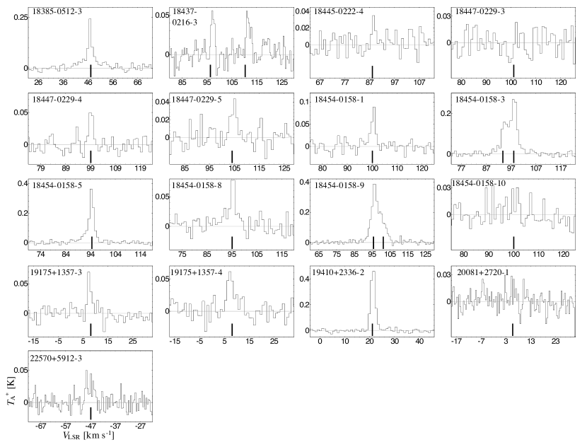
Figure 1: Spectra of HC₃N ($J=9-8$) in HMSCs. The vertical lines indicate the systemic velocities of each source reported by (Sridharan et al., 2005), except for HMSC 18385-0512-3. In the case of HMSC 18385-0512-3, the vertical line corresponds to the $V_{\rm{LSR}}$ value of the $J=5-4$ transition line of HC₃N reported by (Taniguchi et al., 2018b).

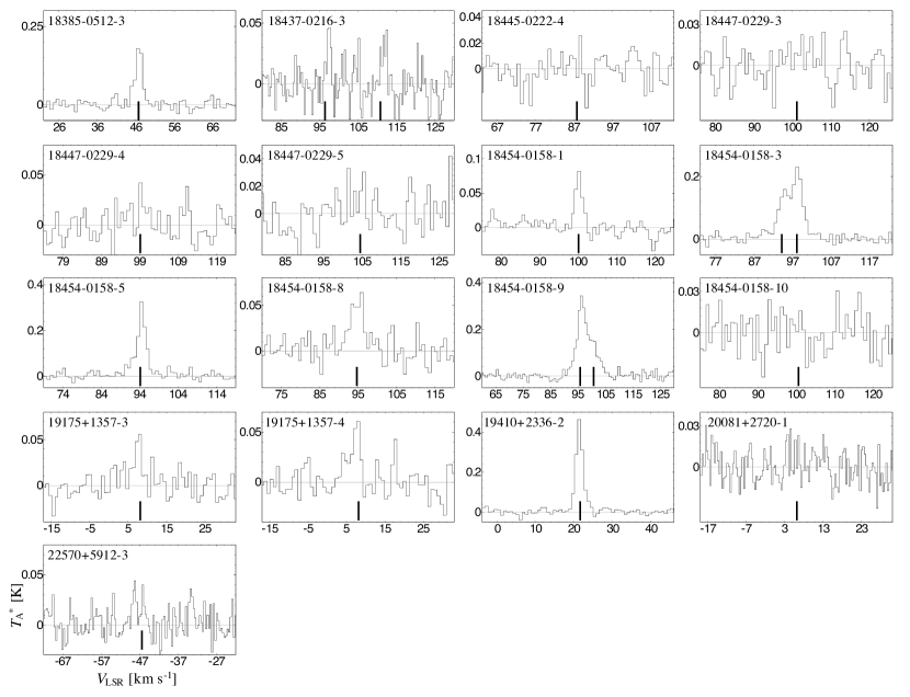
Figure 2: Spectra of HC₃N ($J=10-9$) in HMSCs. The vertical lines indicate the systemic velocities of each source reported by (Sridharan et al., 2005), except for HMSC 18385-0512-3. In the case of HMSC 18385-0512-3, the vertical line corresponds to the $V_{\rm{LSR}}$ value of the $J=5-4$ transition line of HC₃N reported by (Taniguchi et al., 2018b).

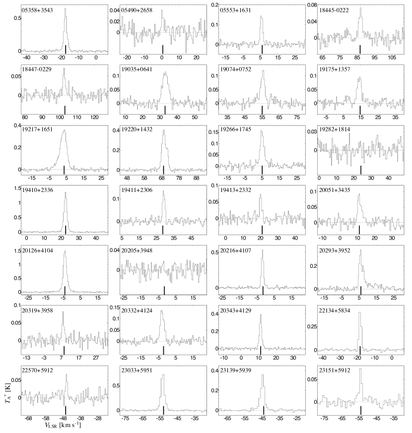
Figure 3: Spectra of HC₃N ($J=9-8$) in HMPOs. The vertical lines indicate the systemic velocities of each source reported by (Sridharan et al., 2002).

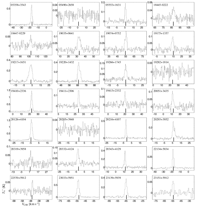
Figure 4: Spectra of HC₃N ($J=10-9$) in HMPOs. The vertical lines indicate the systemic velocities of each source reported by (Sridharan et al., 2002).

Table 2: Spectral line parameters of HC₃N in HMSCs and HMPOs

	HC3N ($J=9-8$)					HC3N ($J=10-9$)
Source	T${}^{\ast}_{\mathrm{A}}$	$\Delta v$	VLSR	$\int T^{\ast}_{\mathrm{A}}dv$	rms		T${}^{\ast}_{\mathrm{A}}$	$\Delta v$	VLSR	$\int T^{\ast}_{\mathrm{A}}dv$	rms
	(K)	(km s-1)	(km s-1)	(K km s-1)	(mK)		(K)	(km s-1)	(km s-1)	(K km s-1)	(mK)
HMSCs
18385-0512-3	0.226 (15)	1.87 (14)	46.8	0.45 (4)	10.9		0.174 (13)	2.4 (2)	46.5	0.44 (5)	13.6
18437-0216-3	0.045 (8)	2.2 (5)	111.0	0.11 (3)	10.4		$<0.045$	…	…	…	15.0
	0.056 (10)	1.4 (3)	97.2	0.09 (2)	10.4		…	…	…	…	15.0
18445-0222-4	0.035 (10)	1.5 (5)	88.6	0.06 (2)	10.4		$<0.036$	…	…	…	11.9
18447-0229-3	$<0.037$	…	…	…	12.3		$<0.037$	…	…	…	12.4
18447-0229-4	0.050 (10)	2.0 (5)	98.9	0.11 (3)	10.4		$<0.047$	…	…	…	15.5
18447-0229-5	0.038 (8)	2.8 (7)	105.1	0.11 (4)	10.4		$<0.043$	…	…	…	14.4
18454-0158-1	0.085 (10)	2.0 (3)	100.8	0.18 (3)	10.4		0.079 (9)	2.1 (3)	100.3	0.18 (3)	11.0
18454-0158-3	0.274 (11)	2.61 (12)	97.9	0.76 (5)	10.1		0.214 (10)	2.92 (16)	98.2	0.66 (5)	12.0
	0.160 (9)	3.3 (3)	94.3	0.57 (5)	10.1		0.149 (9)	3.5 (3)	95.0	0.55 (5)	12.0
18454-0158-5	0.330 (13)	2.43 (11)	94.3	0.85 (5)	9.6		0.284 (14)	2.72 (15)	94.4	0.82 (6)	15.2
18454-0158-8	0.066 (9)	3.4 (5)	95.8	0.24 (5)	11.5		0.055 (8)	4.4 (8)	96.0	0.26 (6)	12.8
18454-0158-9	0.162 (10)	5.6 (5)	99.5	0.96 (10)	10.8		0.180 (9)	8.2 (3)	98.6	1.57 (10)	14.3
	0.346 (13)	3.70 (15)	95.9	1.36 (8)	10.8		0.186 (13)	2.29 (19)	96.2	0.45 (5)	14.3
18454-0158-10	$<0.037$	…	…	…	12.4		$<0.040$	…	…	…	13.2
19175+1357-3	0.070 (11)	1.5 (3)	7.3	0.11 (3)	10.8		0.049 (11)	2.3 (6)	8.1	0.12 (4)	13.2
19175+1357-4	0.060 (9)	3.0 (5)	7.3	0.19 (5)	11.5		0.061 (13)	1.9 (5)	8.1	0.12 (4)	14.2
19410+2336-2	0.448 (19)	2.27 (11)	21.7	1.08 (7)	11.1		0.451 (11)	2.19 (6)	21.3	1.05 (4)	13.3
20081+2720-1	$<0.035$	…	…	…	11.5		$<0.039$	…	…	…	12.9
22570+5912-3	0.048 (11)	1.0 (3)	-48.6	0.05 (2)	10.9		$<0.042$	…	…	…	13.9
HMPOs
05358+3543	0.602 (10)	1.89 (4)	-17.6	1.21 (3)	9.8		0.573 (10)	1.85 (4)	-17.4	1.13 (3)	11.2
05490+2658	0.033 (8)	1.4 (4)	0.2	0.05 (2)	10.4		$<0.041$	…	…	…	13.7
05553+1631	0.151 (8)	1.70 (10)	5.4	0.27 (2)	9.8		0.181 (10)	1.51 (10)	5.7	0.29 (3)	14.1
18445-0222	0.064 (9)	2.4 (3)	87.0	0.16 (3)	10.7		0.048 (6)	3.4 (5)	87.4	0.17 (4)	13.4
18447-0229	0.067 (9)	1.5 (2)	102.6	0.10 (2)	11.0		0.042 (8)	2.3 (5)	102.3	0.11 (3)	13.8
19035+0641	0.113 (5)	4.0 (2)	33.3	0.48 (3)	11.4		0.099 (6)	4.0 (3)	33.1	0.42 (4)	13.1
19074+0752	0.115 (7)	2.7 (2)	55.8	0.33 (3)	11.5		0.124 (8)	2.44 (18)	55.5	0.32 (3)	13.6
19175+1357	0.091 (6)	2.9 (2)	14.5	0.28 (3)	11.2		0.092 (8)	2.6 (3)	14.6	0.26 (3)	9.9
19217+1651	0.336 (10)	4.61 (16)	4.0	1.65 (8)	10.7		0.311 (7)	4.21 (11)	4.1	1.40 (5)	13.7
19220+1432	0.360 (10)	3.30 (10)	69.2	1.26 (5)	10.6		0.365 (10)	3.32 (10)	69.5	1.29 (5)	13.0
19266+1745	0.145 (6)	2.66 (13)	4.6	0.41 (3)	9.5		0.120 (6)	2.74 (17)	4.8	0.35 (3)	11.9
19282+1814	$<0.032$	…	…	…	10.7		$<0.040$	…	…	…	13.3
19410+2336	1.298 (12)	1.97 (2)	22.4	2.72 (4)	11.3		1.359 (13)	1.96 (2)	22.5	2.83 (4)	13.3
19411+2306	0.130 (8)	1.65 (12)	29.0	0.23 (2)	9.8		0.159 (10)	1.63 (11)	29.2	0.28 (3)	13.6
19413+2332	0.077 (9)	1.32 (17)	20.1	0.11 (2)	10.7		0.074 (10)	1.5 (2)	20.2	0.12 (2)	13.5
20051+3435	0.085 (7)	2.5 (2)	11.3	0.23 (3)	11.2		0.098 (10)	1.7 (2)	11.1	0.18 (3)	15.3
20126+4104	1.456 (14)	2.40 (3)	-3.8	3.72 (6)	12.2		1.533 (17)	2.49 (3)	-4.0	4.06 (7)	14.0
20205+3948	$<0.033$	…	…	…	11.0		$<0.041$	…	…	…	13.5
20216+4107	0.539 (10)	1.33 (3)	-1.7	0.76 (2)	11.7		0.558 (13)	1.36 (4)	-1.5	0.81 (3)	13.8
20293+3952	0.281 (12)	2.85 (14)	6.0	0.85 (5)	12.0		0.265 (11)	2.88 (13)	6.2	0.81 (5)	13.4
20319+3958	0.070 (9)	1.5 (2)	8.1	0.11 (2)	12.0		0.044 (7)	3.6 (7)	8.3	0.17 (4)	15.2
20332+4124	0.133 (7)	2.53 (16)	-3.0	0.36 (3)	11.4		0.138 (8)	2.39 (16)	-2.5	0.35 (3)	14.1
20343+4129	0.368 (9)	1.47 (4)	11.3	0.58 (2)	11.0		0.390 (13)	1.53 (6)	11.3	0.64 (3)	16.4
22134+5834	0.409 (15)	1.63 (7)	-18.6	0.71 (4)	10.6		0.421 (14)	1.59 (6)	-18.2	0.71 (3)	13.7
22570+5912	0.066 (10)	1.02 (18)	-46.0	0.07 (2)	11.3		0.065 (11)	1.1 (2)	-45.4	0.08 (2)	13.4
23033+5951	0.69 (3)	2.65 (11)	-53.0	1.95 (11)	10.0		0.67 (2)	2.83 (12)	-52.9	2.00 (11)	12.0
23139+5939	0.342 (9)	2.58 (8)	-44.7	0.94 (4)	8.1		0.356 (13)	2.60 (11)	-44.3	0.99 (5)	12.5
23151+5912	0.074 (8)	1.64 (19)	-54.3	0.13 (2)	7.6		0.059 (10)	1.9 (4)	-54.2	0.12 (3)	10.1

Note. — The numbers in parentheses represent the standard deviation in the Gaussian fit. The errors are written in units of the last significant digit. The upper limits correspond to $3\sigma$ values.

Figures 5 and 6 show the spectra of N₂H⁺ ($J=1-0$) in HMSCs and HMPOs, respectively. Table 3 summarizes the spectral line parameters. We set the $F_{1}=2-1$ transition as the criteria of velocity, and the $V_{\rm{LSR}}$ values are consistent with those of HC₃N within their errors. N₂H⁺ was detected in all of the target sources except for HMPO 23151+5912 with an S/N ratio above 4. Seven hyperfine components were detected as three lines. In some sources, we cannot clearly identify lines due to blending two velocity components.

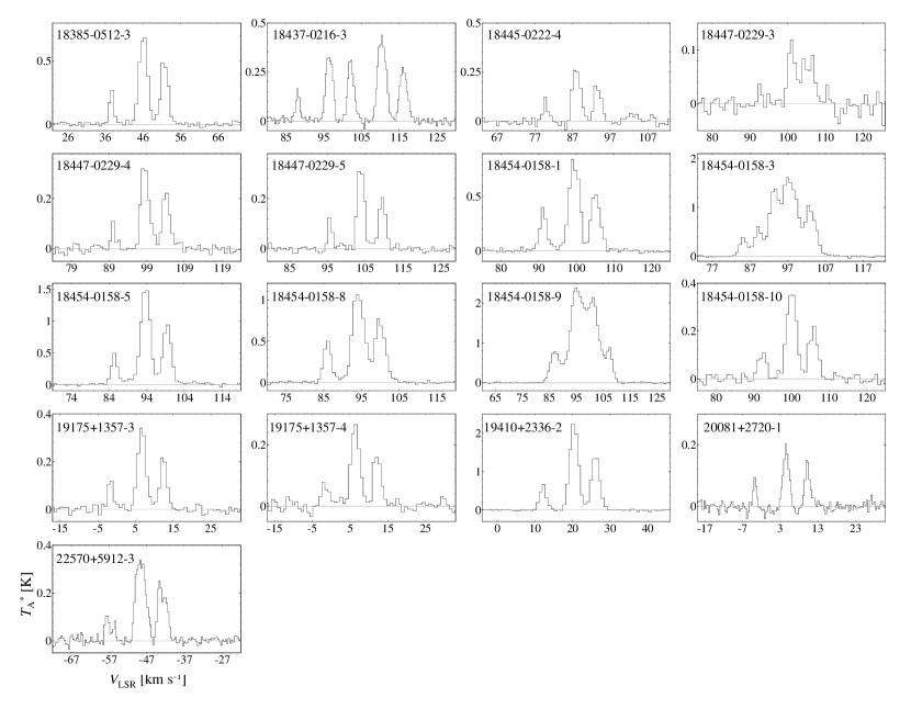
Figure 5: Spectra of N₂H⁺ ($J=1-0$) in HMSCs.

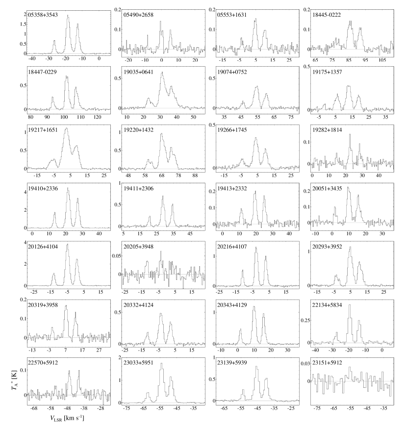
Figure 6: Spectra of N₂H⁺ ($J=1-0$) in HMPOs.

Table 3: Spectral line parameters of N₂H⁺ ($J=1-0$) in HMSCs and HMPOs

Source	Hyperfine	T${}^{\ast}_{\rm A}$	$\Delta v$	VLSR	$\int T^{\ast}_{\rm A}dv$	rms
	transition	(K)	(km/s)	(km/s)	(K km/s)	(mK)
HMSCs
18385-0512-3	$F_{1}=1-1$	0.507 (15)	2.34 (8)	51.7	1.26 (6)	14.7
	$F_{1}=2-1$	0.724 (14)	2.63 (6)	46.0	2.03 (6)
	$F_{1}=0-0$	0.29 (2)	1.33 (11)	37.6	0.41 (5)
18437-0216-3		0.269 (9)	2.27 (9)	116.1	0.65 (3)	13.0
		0.436 (9)	2.52 (6)	110.4	1.17 (4)
		0.308 (10)	1.92 (7)	102.2	0.63 (3)
		0.350 (10)	2.16 (7)	96.5	0.80 (3)
		0.156 (13)	1.21 (11)	88.1	0.20 (3)
18445-0222-4	$F_{1}=1-1$	0.185 (15)	2.2 (2)	93.6	0.43 (5)	14.2
	$F_{1}=2-1$	0.279 (14)	2.47 (14)	88.1	0.73 (6)
	$F_{1}=0-0$	0.122 (18)	1.3 (2)	79.8	0.17 (3)
18447-0229-3	$F_{1}=1-1$ ?	0.078 (9)	4.4 (7)	105.4	0.37 (7)	13.8
	$F_{1}=2-1$ ?	0.116 (13)	2.0 (3)	100.9	0.24 (4)
18447-0229-4	$F_{1}=1-1$	0.226 (12)	2.34 (14)	104.1	0.56 (5)	13.3
	$F_{1}=2-1$	0.334 (11)	2.59 (10)	98.4	0.92 (5)
	$F_{1}=0-0$	0.110 (15)	1.15 (16)	90.1	0.13 (3)
18447-0229-5	$F_{1}=1-1$	0.209 (11)	2.14 (12)	109.6	0.48 (3)	11.0
	$F_{1}=2-1$	0.337 (10)	2.17 (7)	103.8	0.78 (3)
	$F_{1}=0-0$	0.133 (13)	1.19 (13)	95.7	0.17 (2)
18454-0158-1	$F_{1}=1-1$	0.539 (17)	2.82 (11)	105.1	1.62 (8)	13.2
	$F_{1}=2-1$	0.858 (16)	3.15 (7)	99.4	2.87 (8)
	$F_{1}=0-0$	0.39 (2)	2.09 (12)	91.2	0.87 (7)
18454-0158-3		0.94 (2)	3.35 (10)	103.1	3.36 (13)	13.4
		1.610 (19)	4.92 (10)	97.4	8.4 (2)
		1.16 (3)	2.47 (7)	93.2	3.07 (12)
		0.58 (3)	2.62 (15)	89.3	1.63 (12)
		0.38 (3)	2.3 (2)	85.3	0.94 (10)
18454-0158-5	$F_{1}=1-1$	0.946 (17)	2.62 (5)	99.4	2.64 (7)	14.7
	$F_{1}=2-1$	1.548 (16)	2.94 (3)	93.7	4.83 (8)
	$F_{1}=0-0$	0.477 (19)	1.96 (9)	85.4	0.99 (6)
18454-0158-8	$F_{1}=1-1$	0.749 (16)	3.30 (9)	99.9	2.63 (9)	12.1
	$F_{1}=2-1$	1.108 (16)	3.63 (6)	94.2	4.28 (9)
	$F_{1}=0-0$	0.502 (19)	2.40 (10)	86.0	1.28 (7)
18454-0158-9		0.79 (3)	2.94 (13)	107.3	2.48 (14)	11.0
		2.00 (2)	5.62 (9)	101.0	12.0 (2)
		2.34 (2)	5.28 (7)	95.0	13.1 (2)
		0.78 (2)	4.17 (16)	87.2	3.48 (17)
18454-0158-10	$F_{1}=1-1$	0.210 (11)	2.82 (18)	105.8	0.63 (5)	13.9
	$F_{1}=2-1$	0.373 (11)	3.07 (10)	100.0	1.22 (5)
	$F_{1}=0-0$	0.108 (12)	2.6 (3)	92.2	0.30 (5)
19175+1357-3	$F_{1}=1-1$	0.225 (10)	2.14 (11)	12.4	0.51 (4)	11.7
	$F_{1}=2-1$	0.351 (10)	2.52 (8)	6.7	0.94 (4)
	$F_{1}=0-0$	0.133 (12)	1.57 (17)	-1.6	0.22 (3)
19175+1357-4	$F_{1}=1-1$	0.172 (11)	2.39 (18)	12.1	0.44 (4)	14.3
	$F_{1}=2-1$	0.269 (11)	2.72 (12)	6.4	0.78 (5)
	$F_{1}=0-0$	0.070 (11)	2.5 (4)	-1.6	0.19 (5)
19410+2336-2	$F_{1}=1-1$	1.422 (16)	2.51 (3)	26.1	3.80 (6)	13.7
	$F_{1}=2-1$	2.274 (15)	2.71 (2)	20.4	6.55 (7)
	$F_{1}=0-0$	0.646 (17)	2.04 (6)	12.1	1.40 (6)
20081+2720-1	$F_{1}=1-1$	0.149 (9)	1.46 (11)	10.2	0.23 (2)	12.0
	$F_{1}=2-1$	0.191 (8)	1.85 (9)	4.6	0.38 (2)
	$F_{1}=0-0$	0.094 (11)	0.97 (14)	-3.4	0.10 (2)
22570+5912-3	$F_{1}=1-1$	0.228 (11)	2.81 (16)	-42.9	0.68 (5)	13.5
	$F_{1}=2-1$	0.354 (11)	3.02 (11)	-48.6	1.14 (5)
	$F_{1}=0-0$	0.084 (12)	2.5 (4)	-57.1	0.22 (5)
HMPOs
05358+3543	$F_{1}=1-1$	1.42 (2)	2.08 (3)	-12.8	3.14 (7)	10.7
	$F_{1}=2-1$	1.950 (18)	2.51 (3)	-18.4	5.21 (7)
	$F_{1}=0-0$	0.67 (2)	1.59 (6)	-27.0	1.13 (6)
05490+2658	$F_{1}=1-1$	0.092 (17)	1.5 (3)	5.3	0.14 (4)	14.8
	$F_{1}=2-1$	0.107 (13)	2.0 (3)	-0.3	0.23 (4)
	$F_{1}=0-0$	0.07 (3)	0.4 (2)	-8.7	0.03 (2)
05553+1631	$F_{1}=1-1$	0.102 (8)	2.2 (2)	10.3	0.24 (3)	13.8
	$F_{1}=2-1$	0.156 (8)	2.22 (13)	4.6	0.37 (3)
	$F_{1}=0-0$	0.050 (9)	1.7 (4)	-3.6	0.09 (2)
18445-0222	$F_{1}=1-1$	0.106 (9)	2.7 (3)	91.8	0.30 (4)	13.7
	$F_{1}=2-1$	0.140 (8)	3.3 (2)	85.8	0.50 (4)
18447-0229	$F_{1}=1-1$	0.430 (13)	2.45 (9)	107.5	1.12 (5)	13.7
	$F_{1}=2-1$	0.727 (13)	2.42 (5)	101.8	1.87 (5)
	$F_{1}=0-0$	0.253 (16)	1.54 (12)	93.4	0.41 (4)
19035+0641	$F_{1}=1-1$	0.316 (7)	5.36 (16)	36.8	1.80 (7)	11.9
	$F_{1}=2-1$	0.566 (9)	3.40 (6)	31.4	2.05 (5)
	$F_{1}=0-0$	0.148 (8)	3.6 (2)	23.5	0.57 (5)
19074+0752	$F_{1}=1-1$	0.246 (9)	2.62 (11)	60.2	0.68 (4)	13.6
	$F_{1}=2-1$	0.381 (8)	3.17 (8)	54.3	1.28 (4)
	$F_{1}=0-0$	0.102 (10)	2.1 (2)	46.2	0.23 (3)
19175+1357	$F_{1}=1-1$	0.164 (9)	2.50 (16)	18.9	0.44 (40	12.8
	$F_{1}=2-1$	0.293 (8)	3.19 (10)	12.9	0.99 (4)
	$F_{1}=0-0$	0.162 (8)	3.00 (18)	6.0	0.52 (4)
19217+1651	$F_{1}=1-1$	0.640 (8)	3.58 (6)	8.4	2.44 (5)	13.8
	$F_{1}=2-1$	1.117 (7)	4.57 (4)	2.5	5.43 (6)
	$F_{1}=0-0$	0.264 (8)	4.07 (14)	-5.7	1.14 (5)
19220+1432		0.503 (15)	4.15 (15)	74.2	2.22 (10)	13.1
		0.936 (16)	3.41 (7)	68.4	3.39 (9)
		0.18 (3)	1.4 (2)	62.1	0.28 (6)
		0.25 (2)	2.0 (2)	59.9	0.53 (7)
19266+1745	$F_{1}=1-1$	0.212 (7)	2.91 (11)	9.7	0.66 (3)	12.2
	$F_{1}=2-1$	0.356 (7)	3.18 (7)	4.0	1.20 (3)
	$F_{1}=0-0$	0.090 (6)	4.0 (3)	-4.2	0.39 (4)
19282+1814	$F_{1}=1-1$	0.083 (12)	1.12 (19)	28.5	0.10 (2)	13.6
	$F_{1}=2-1$	0.107 (10)	1.63 (17)	22.7	0.19 (3)
	$F_{1}=0-0$	0.043 (12)	1.1 (4)	14.6	0.05 (2)
19410+2336	$F_{1}=1-1$	3.10 (4)	2.04 (3)	27.3	6.73 (12)	14.5
	$F_{1}=2-1$	4.44 (3)	2.47 (2)	21.6	11.69 (13)
	$F_{1}=0-0$	1.64 (4)	1.50 (4)	13.4	2.61 (10)
19411+2306	$F_{1}=1-1$	0.489 (16)	1.57 (6)	34.5	0.82 (4)	16.3
	$F_{1}=2-1$	0.651 (13)	2.16 (5)	28.7	1.50 (5)
	$F_{1}=0-0$	0.224 (17)	1.34 (12)	20.6	0.32 (4)
19413+2332	$F_{1}=1-1$	0.166 (9)	1.78 (11)	25.1	0.31 (3)	13.1
	$F_{1}=2-1$	0.204 (8)	2.03 (9)	19.5	0.44 (3)
	$F_{1}=0-0$	0.094 (9)	1.65 (18)	11.3	0.17 (2)
20051+3435	$F_{1}=1-1$	0.146 (8)	2.53 (16)	15.7	0.39 (3)	14.7
	$F_{1}=2-1$	0.226 (8)	2.50 (11)	10.0	0.60 (3)
	$F_{1}=0-0$	0.090 (10)	1.7 (2)	1.8	0.16 (3)
20126+4104	$F_{1}=1-1$	2.431 (18)	2.25 (2)	0.9	5.82 (6)	12.9
	$F_{1}=2-1$	3.855 (17)	2.49 (1)	-4.8	10.20 (7)
	$F_{1}=0-0$	1.15 (2)	1.83 (4)	-13.1	2.23 (6)
20205+3948	$F_{1}=2-1$	0.050 (10)	1.6 (4)	-3.4	0.08 (2)	14.3
	$F_{1}=0-0$	0.039 (10)	1.5 (4)	-11.9	0.06 (2)
20216+4107	$F_{1}=1-1$	0.973 (16)	1.77 (3)	3.0	1.83 (5)	14.2
	$F_{1}=2-1$	1.353 (15)	2.09 (3)	-2.7	3.00 (5)
	$F_{1}=0-0$	0.55 (2)	1.19 (5)	-11.0	0.70 (4)
20293+3952	$F_{1}=1-1$	0.657 (19)	3.02 (10)	10.6	2.11 (9)	15.3
	$F_{1}=2-1$	1.094 (19)	2.90 (6)	4.8	3.37 (9)
	$F_{1}=0-0$	0.28 (2)	2.8 (2)	-3.3	0.81 (9)
20319+3958	$F_{1}=1-1$	0.118 (9)	1.88 (17)	12.9	0.24 (3)	13.6
	$F_{1}=2-1$	0.177 (9)	2.05 (12)	7.3	0.39 (3)
	$F_{1}=0-0$	0.058 (11)	1.2 (3)	-1.0	0.08 (2)
20332+4124	$F_{1}=1-1$	0.335 (9)	2.58 (8)	2.3	0.92 (4)	13.4
	$F_{1}=2-1$	0.496 (8)	2.76 (5)	-3.4	1.45 (4)
	$F_{1}=0-0$	0.172 (9)	2.15 (14)	-11.6	0.39 (3)
20343+4129	$F_{1}=1-1$	0.936 (14)	1.88 (3)	15.7	1.87 (4)	13.5
	$F_{1}=2-1$	1.236 (12)	2.28 (3)	10.0	3.00 (5)
	$F_{1}=0-0$	0.468 (15)	1.51 (6)	1.7	0.75 (4)
22134+5834	$F_{1}=1-1$	0.259 (11)	1.94 (10)	-13.7	0.53 (3)	11.9
	$F_{1}=2-1$	0.413 (11)	2.12 (6)	-19.4	0.93 (4)
	$F_{1}=0-0$	0.111 (12)	1.7 (2)	-27.5	0.20 (3)
22570+5912	$F_{1}=1-1$	0.088 (11)	1.31 (19)	-41.1	0.12 (2)	13.7
	$F_{1}=2-1$	0.094 (9)	1.8 (2)	-46.7	0.18 (3)
	$F_{1}=0-0$	0.037 (12)	1.0 (4)	-55.1	0.04 (2)
23033+5951	$F_{1}=1-1$	1.097 (17)	2.94 (5)	-48.4	3.43 (8)	13.5
	$F_{1}=2-1$	1.745 (16)	3.13 (3)	-54.1	5.81 (8)
	$F_{1}=0-0$	0.465 (18)	2.53 (11)	-62.3	1.25 (7)
23139+5939	$F_{1}=1-1$	0.530 (13)	2.58 (7)	-39.8	1.45 (5)	11.0
	$F_{1}=2-1$	0.796 (12)	2.89 (5)	-45.5	2.45 (6)
	$F_{1}=0-0$	0.252 (15)	1.74 (12)	-53.7	0.47 (4)
23151+5912		$<0.030$	…	…	…	9.6

Note. — The numbers in parentheses represent the standard deviation in the Gaussian fit. The errors are written in units of the last significant digit. The upper limits correspond to $3\sigma$ values.

Figures 7 and 8 show spectra of c-C₃H₂ and CCS detected with an S/N ratio above 3, including tentative detection, respectively. The spectral line parameters obtained from the Gaussian fitting are summarized in Table 4. c-C₃H₂ was detected in 15 HMSCs and 19 HMPOs and CCS was detected in 2 HMSCs and 13 HMPOs.

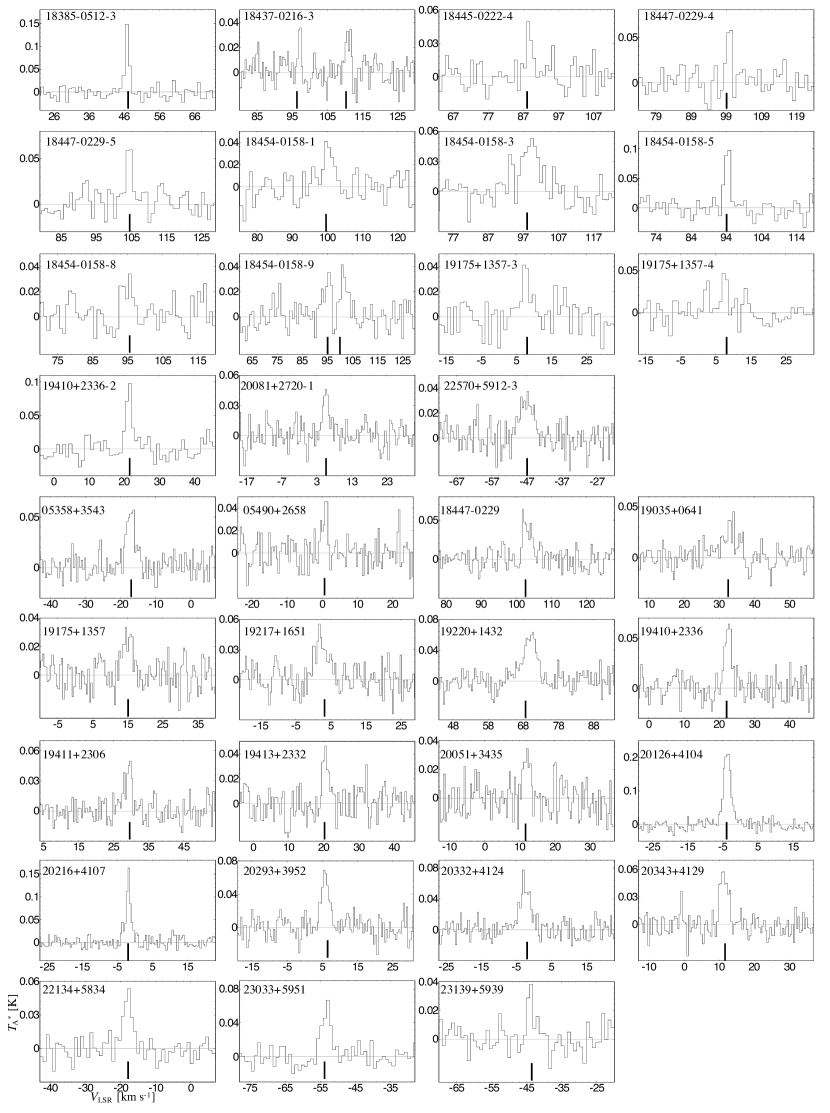
Figure 7: Spectra of c-C₃H₂ ($J_{\rm Ka,Kc}=2_{0,2}-1_{1,1}$) in HMSCs and HMPOs. The vertical lines indicate the systemic velocities of each source reported by (Sridharan et al., 2002, 2005), except for HMSC 18385-0512-3. In the case of HMSC 18385-0512-3, the vertical line corresponds to the $V_{\rm{LSR}}$ value of the $J=5-4$ transition line of HC₃N reported by (Taniguchi et al., 2018b).

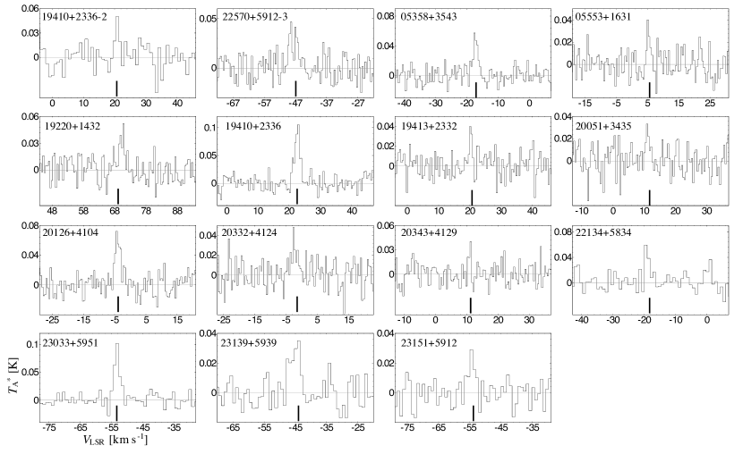
Figure 8: Spectra of CCS ($J_{\rm N}=6_{7}-5_{6}$) in HMSCs and HMPOs. The vertical lines indicate the systemic velocities of each source reported by (Sridharan et al., 2002, 2005).

Table 4: Spectral line parameters c-C₃H₂ ($J_{\rm Ka,Kc}=2_{0,2}-1_{1,1}$) and CCS ($J_{\rm N}=6_{7}-5_{6}$)

	c-C3H2 ($J_{\rm Ka,Kc}=2_{0,2}-1_{1,1}$)					CCS ($J_{\rm N}=6_{7}-5_{6}$)
Source	T${}^{\ast}_{\mathrm{A}}$	$\Delta v$	VLSR	$\int T^{\ast}_{\mathrm{A}}dv$	rms		T${}^{\ast}_{\mathrm{A}}$	$\Delta v$	VLSR	$\int T^{\ast}_{\mathrm{A}}dv$	rms
	(K)	(km s-1)	(km s-1)	(K km s-1)	(mK)		(K)	(km s-1)	(km s-1)	(K km s-1)	(mK)
HMSCs
18385-0512-3	0.148 (11)	1.38 (11)	46.7	0.22 (2)	10.6		…	$<0.036$	…	…	11.9
18437-0216-3	0.032 (8)	1.6 (5)	111.7	0.05 (2)	10.1		$<0.034$	…	…	…	11.4
	0.036 (10)	0.9 (3)	97.4	0.04 (2)			…	…	…	…
18445-0222-4	0.044 (10)	2.1 (5)	88.4	0.10 (3)	10.9		$<0.039$	…	…	…	13.1
18447-0229-4	0.055 (12)	1.7 (4)	100.5	0.10 (3)	11.1		$<0.039$	…	…	…	13.0
18447-0229-5	0.058 (11)	2.2 (5)	104.9	0.14 (4)	11.4		$<0.036$	…	…	…	11.9
18454-0158-1	0.038 (8)	3.4 (8)	99.6	0.13 (4)	10.7		$<0.032$	…	…	…	10.7
18454-0158-3	0.047 (7)	5.9 (9)	99.5	0.30 (6)	11.8		$<0.034$	…	…	…	11.3
18454-0158-5	0.092 (12)	2.1 (3)	94.9	0.21 (4)	11.6		$<0.034$	…	…	…	11.3
18454-0158-8	0.027 (8)	3.4 (1.1)	95.6	0.10 (4)	10.0		$<0.033$	…	…	…	11.0
18454-0158-9	0.036 (9)	3.0 (9)	101.1	0.11 (4)	10.6		$<0.034$	…	…	…	11.3
	0.038 (11)	2.0 (7)	95.7	0.08 (4)	10.6		…	…	…	…
19175+1357-3	0.036 (9)	3.1 (9)	7.3	0.12 (4)	11.2		$<0.034$	…	…	…	11.4
19175+1357-4	0.048 (11)	1.8 (5)	7.3	0.09 (3)	12.2		$<0.049$	…	…	…	12.3
19410+2336-2	0.092 (11)	2.2 (3)	21.6	0.21 (4)	12.1		0.051 (14)	1.5 (4)	20.8	0.08 (3)	13.7
20081+2720-1	0.045 (7)	2.0 (4)	5.7	0.10 (2)	10.9		$<0.032$	…	…	…	10.5
22570+5912-3	0.031 (4)	4.4 (7)	-46.7	0.15 (3)	10.6		0.031 (6)	3.7 (8)	-48.4	0.12 (3)	11.4
HMPOs
05358+3543	0.052 (5)	3.3 (4)	-16.3	0.18 (3)	9.7		0.047 (6)	2.0 (3)	-17.5	0.10 (2)	9.6
05490+2658	0.046 (9)	1.4 (3)	1.0	0.07 (2)	11.5		$<0.037$	…	…	…	12.2
05553+1631	$<0.030$	…	…	…	10.0		0.038 (10)	1.0 (3)	5.1	0.04 (1)	10.0
18447-0229	0.054 (8)	1.8 (3)	102.0	0.10 (2)	11.1		$<0.033$	…	…	…	11.1
19035+0641	0.026 (4)	4.9 (9)	34.1	0.14 (3)	9.8		$<0.035$	…	…	…	11.6
19175+1357	0.028 (5)	3.3 (7)	14.5	0.10 (3)	9.8		$<0.032$	…	…	…	10.5
19217+1651	0.041 (6)	4.1 (7)	1.8	0.18 (4)	11.9		$<0.035$	…	…	…	11.8
19220+1432	0.056 (5)	4.4 (5)	70.8	0.27 (4)	10.3		0.035 (7)	2.4 (6)	70.8	0.09 (3)	11.6
19410+2336	0.062 (7)	2.3 (3)	22.8	0.15 (3)	11.0		0.088 (8)	2.1 (2)	23.0	0.20 (3)	11.5
19411+2306	0.038 (6)	2.7 (5)	29.8	0.11 (3)	9.3		$<0.031$	…	…	…	10.4
19413+2332	0.042 (7)	2.0 (4)	20.6	0.09 (2)	10.5		0.040 (10)	1.0 (3)	20.1	0.04 (2)	11.5
20051+3435	0.032 (7)	2.1 (5)	12.2	0.07 (2)	10.9		0.031 (10)	1.3 (5)	10.9	0.04 (2)	11.8
20126+4104	0.219 (7)	2.45 (10)	-3.3	0.57 (3)	11.8		0.061 (8)	2.3 (4)	-4.3	0.15 (3)	12.4
20216+4107	0.145 (9)	1.41 (10)	-1.7	0.22 (2)	10.9		$<0.040$	…	…	…	13.3
20293+3952	0.063 (7)	2.6 (3)	5.6	0.17 (3)	11.3		$<0.040$	…	…	…	13.4
20332+4124	0.056 (5)	3.6 (4)	-2.9	0.21 (3)	11.6		0.030 (8)	2.5 (8)	-2.6	0.08 (3)	13.2
20343+4129	0.059 (8)	2.6 (3)	11.3	0.16 (3)	11.0		0.040 (12)	0.5 (2)	11.3	0.02 (1)	12.2
22134+5834	0.049 (7)	3.0 (5)	-17.6	0.16 (3)	10.1		0.059 (13)	1.2 (3)	-19.5	0.08 (3)	11.7
23033+5951	0.059 (8)	3.1 (5)	-52.8	0.19 (4)	10.5		0.098 (9)	2.1 (2)	-53.2	0.21 (3)	10.0
23139+5939	0.035 (7)	2.2 (5)	-43.7	0.08 (3)	8.0		0.031 (8)	3.2 (9)	-44.0	0.10 (4)	9.6
23151+5912	$<0.027$	…	…	…	9.3		0.026 (7)	2.3 (7)	-54.5	0.06 (3)	8.6

Note. — The numbers in parentheses represent the standard deviation in the Gaussian fit. The errors are written in units of the last significant digit. The upper limits correspond to $3\sigma$ values.

4 Analyses

4.1 Column Densities and Rotational Temperatures of HC₃N

We derived the rotational temperatures and column densities of HC₃N from the rotational diagram analysis, using the following formula (Goldsmith & Langer, 1999);

$${\rm{ln}}\frac{3k\int T_{\mathrm{mb}}dv}{8\pi^{3}\nu S\mu^{2}}={\rm{ln}}\frac{N}{Q(T_{\rm{rot}})}-\frac{E_{\rm{u}}}{kT_{\rm{rot}}},$$ (1)

where $k$ is the Boltzmann constant, $S$ is the line strength, $\mu$ is the permanent electric dipole moment, $N$ is the column density, and $Q(T_{\rm{rot}})$ is the partition function. The permanent electric dipole moment is 3.7312 D for HC₃N (Deleon & Muenter, 1985). We combined the $J=9-8$ and $10-9$ data with the $J=5-4$ transition (45.49031 GHz, $E_{\rm{u}}/k=6.5$ K) obtained with the Nobeyama 45-m telescope (Taniguchi et al., 2018b).

We derived the column densities assuming two cases. First, assuming that emission regions of HC₃N is much larger than a beam size at 45 GHz with the Nobeyama 45-m telescope ($37\arcsec$), we analyzed the data without the beam size correction. Second, we multiplied the integrated intensities of the $J=5-4$ data by ($\frac{37\arcsec}{18\arcsec}$)² for the beam size correction, assuming small beam filling factors. We assume that the emission-region size of HC₃N is $5\arcsec$, which is much smaller than $18\arcsec$. We apply this assumption based on previous observations of HC₃N toward massive young stellar objects (Taniguchi et al., 2018a). We summarize the derived rotational temperatures and column densities by the above two assumptions in Table 5. The rotational temperatures in some sources with the beam size correction are lower than a typical value in low-mass starless dark clouds (6.5 K; Suzuki et al., 1992), which are unlikely results. These low rotational temperatures possibly imply the non-LTE or opacity effects. We thus use values without the beam size correction in the following sections. In some sources, the rotational temperatures derived without the beam size correction are significantly higher (e.g., $T_{\rm{rot}}=370$ K in HMPO 05553+1631) compared to other sources. However, the rotational temperatures derived with beam size correction seem to be reasonable (e.g., $T_{\rm{rot}}=11$ K in HMPO 05553+1631). This implies that emission regions are small.

Table 5: Rotational temperatures and column densities of HC₃N

	Without beam-size correction			With beam-size correction
Source	$T_{\rm{rot}}$	$N$		$T_{\rm{rot}}$	$N$
	(K)	($\times 10^{12}$ cm-2)		(K)	($\times 10^{12}$ cm-2)
HMSCs
18385-0512-3	10 (3)	4.9 (1.5)		5.3 (1.6)	18 (5
18437-0216-3
($V_{\rm{LSR}}$ = 111.0 km/s)	8 (3)	1.3 (0.4)		4.4 (1.3)	5.7 (1.8)
18445-0222-4	13 (4)	0.47 (0.14)		5.4 (1.6)	1.6 (0.5)
18447-0229-4	7 (2)	1.9 (0.6)		3.9 (1.2)	9 (3)
18447-0229-5	13 (4)	0.9 (0.3)		5.3 (1.6)	3.4 (1.1)
18454-0158-1	11 (3)	1.8 (0.6)		5.6 (1.7)	6 (2)
18454-0158-3
($V_{\rm{LSR}}$ = 97.9 km/s)	8 (2)	12 (3)		4.6 (1.4)	50 (15)
18454-0158-5	11 (3)	9 (2)		5.5 (1.6)	33 (10)
18454-0158-8	10 (3)	2.7 (0.8)		5.4 (1.6)	10 (3)
18454-0158-9
($V_{\rm{LSR}}$ = 99.5 km/s)	24 (7)	9 (3)		8 (2)	22 (7)
($V_{\rm{LSR}}$ = 95.9 km/s)	9 (3)	10 (3)		5.0 (1.5)	38 (12)
19175+1357-3	12 (3)	1.1 (0.3)		5.7 (1.7)	3.9 (1.2)
19175+1357-4	12 (3)	1.4 (0.4)		5.7 (1.7)	5.0 (1.5)
19410+2336-2	22 (7)	8 (2)		7 (2)	19 (6)
22570+5912-3	6.3 (1.9)	0.9 (0.3)		3.7 (1.1)	4.8 (1.5)
HMPOs
05358+3543	16 (5)	9 (3)		7 (2)	28 (8)
05490+2658	11 (3)	0.47 (0.15)		4.9 (1.5)	1.9 (0.6)
05553+1631	370	13.6		11 (3)	2.9 (0.9)
18445-0222	8 (2)	2.4 (0.7)		4.8 (1.4)	10 (3)
18447-0229	12 (4)	1.0 (0.3)		5.9 (1.8)	3.3 (1.0)
19035+0641	11 (3)	4.4 (1.4)		5.6 (1.7)	16 (5)
19074+0752	25 (7)	2.4 (0.7)		8 (2)	5.4 (1.7)
19175+1357	109	4.38		10 (3)	2.9 (0.9)
19217+1651	21 (6)	11 (3)		7 (2)	27 (8)
19220+1432	32 (9)	10 (3)		8 (2)	19 (6)
19266+1745	10 (3)	4.1 (1.3)		5.4 (1.6)	15 (4)
19410+2336	35 (10)	23 (7)		9 (2)	39 (12)
19411+2306	11 (3)	2.5 (0.7)		5.6 (1.7)	9 (3)
19413+2332	9 (3)	1.5 (0.5)		4.9 (1.5)	6.1 (1.9)
20051+3435	12 (3)	1.9 (0.6)		5.7 (1.7)	7 (2)
20126+4104	…	…		13(4)	35 (10)
20216+4107	51 (15)	8 (2)		9 (3)	10 (3)
20293+3952	17 (5)	6.4 (1.9)		7 (2)	18 (6)
20319+3958	19 (6)	1.0 (0.3)		7 (2)	2.7 (0.8)
20332+4124	12 (4)	3.2 (0.9)		5.9 (1.8)	11 (3)
20343+4129	15 (4)	5.0 (1.5)		6.4 (1.9)	15 (5)
22134+5834	10 (3)	8 (2)		5.3 (1.6)	31 (9)
22570+5912	7 (2)	1.5 (0.5)		4.3 (1.3)	7 (2)
23033+5951	24 (7)	15 (4)		8 (2)	33 (10)
23139+5939	27 (8)	7 (2)		8 (2)	15 (5)
23151+5912	13 (4)	1.1 (0.3)		6.1 (1.8)	3.5 (1.1)

Note. — The numbers in parentheses represent the standard deviation.

4.2 Column Densities and Excitation Temperatures of N₂H⁺

We derived the column densities and excitation temperatures of N₂H⁺ from the LTE analysis. In case that the spectral line parameters of the three hyperfine components ($F_{1}=1-1$, $2-1$, and $0-0$) were obtained, we followed the procedure and used formulae derived in Appendix B1 by Furuya et al. (2006). For the calculation, we used the values obtained by the Gaussian fitting (Table 3). We assume that all of the hyperfine components have the same thermal and non-thermal line broadenings. This can be applicable because all of these lines should come from the same emission region. We used the line width of $F_{1}=0-0$ as the intrinsic line width, because this component is not blended and consists of only one component. The derived excitation temperature, optical depth, and column density are summarized in Table 6. In some sources, we cannot derive its excitation temperatures and column densities from the simultaneous hyperfine-component fitting. In that case, we derived its column densities using the $F_{1}=2-1$ component (the central strongest line) and the formula (97) in Mangum & Shirley (2015), assuming that its excitation temperature is equal to the average values in HMSCs (4.0 K) and HMPOs (4.7 K), respectively.

The derived excitation temperatures of N₂H⁺ are lower than the rotational temperatures of NH₃ (Sridharan et al., 2002, 2005) or HC₃N (Table 5). Sakai et al. (2008) derived the excitation temperatures of N₂H⁺ in massive clumps. Their results also show that the excitation temperatures of N₂H⁺ are lower than the rotational temperatures of NH₃. These results seem to suggest that N₂H⁺ trace colder regions in massive clumps compared to NH₃.

Table 6: Excitation temperatures, optical depth, and column densities of N₂H⁺

Source	$T_{\rm{ex}}$	$\tau$	$N$
	(K)		($\times 10^{13}$ cm-2)
HMSCs
18385-0512-3	3.9 (0.3)	6.3 (0.6)	1.89 (0.16)
18445-0222-4	3.1 (0.6)	8.8 (1.6)	1.9 (0.3)
18447-0229-3	4.0		0.18 (0.04)
18447-0229-4	3.4 (0.5	4.0 (0.6)	0.86 (0.13)
18447-0229-5	3.2 (0.4)	8.1 (1.0)	1.7 (0.2)
18454-0158-1	3.9 (0.3)	11.0 (0.8)	5.2 (0.4)
18454-0158-5	5.3 (0.3)	4.4 (0.2)	3.02 (0.15)
18454-0158-8	4.4 (0.2)	9.2 (0.5)	5.9 (0.3)
18454-0158-10	3.3 (0.4)	4.7 (0.6)	2.2 (0.3)
19175+1357-3	3.3 (0.4)	6.8 (0.8)	1.9 (0.2)
19175+1357-4	3.6 (0.7)	1.9 (0.4)	0.98 (0.18)
19410+2336-2	7.1 (0.2)	3.2 (0.1)	3.62 (0.12)
20081+2720-1	3.1 (0.5)	7.9 (1.2)	1.3 (0.2)
22570+5912-3	4.7 (0.8)	0.90 (0.14)	0.66 (0.11)
HMPOs
05358+3543	6.8 (0.3)	3.60 (0.15)	2.95 (0.12)
05490+2658	4.7		0.14 (0.07)
05553+1631	3.7 (0.8)	0.80 (0.17)	0.28 (0.06)
18445-0222	3.1 (0.5)	2.6 (0.4)	1.15 (0.18)
18447-0229	3.8 (0.3)	6.7 (0.5)	2.24 (0.18)
19035+0641	3.7 (0.3)	3.5 (0.2)	2.66 (0.18)
19074+0752	5.2 (0.6)	0.70 (0.08)	0.51 (0.05)
19175+1357	4.7		0.60 (0.05)
19217+1651	5.3 (0.2)	2.1 (0.1)	2.99 (0.11)
19266+1745	3.6 (0.3)	2.4 (0.2)	1.41 (0.11)
19282+1814	3.0 (1.1)	4.9 (1.7)	0.9 (0.3)
19410+2336	10.1 (0.3)	5.10 (0.16)	7.6 (0.2)
19411+2306	4.3 (0.4)	3.3 (0.3)	1.14 (0.11)
19413+2332	3.1 (0.4)	6.2 (0.8)	1.7 (0.2)
20051+3435	3.1 (0.4)	7.6 (1.1)	2.1 (0.3)
20126+4104	9.6 (0.2)	3.60 (0.07)	6.04 (0.12)
20205+3948	4.7		0.05 (0.02)
20216+4107	5.0 (0.2)	6.2 (0.3)	2.37 (0.10)
20293+3952	5.2 (0.4)	2.3 (0.2)	2.16 (0.18)
20319+3958	3.1 (0.7)	4.1 (0.9)	0.84 (0.19)
20332+4124	3.6 (0.2)	4.6 (0.3)	2.00 (0.14)
20343+4129	5.3 (0.2)	4.30 (0.17)	2.27 (0.09)
22134+5834	3.7 (0.5)	2.4 (0.3)	0.85 (0.11)
22570+5912	3.1 (1.2)	2.3 (0.9)	0.40 (0.16)
23033+5951	6.7 (0.3)	2.40 (0.11)	3.07 (0.14)
23139+5939	4.3 (0.3)	3.7 (0.3)	1.66 (0.12)

Note. — The numbers in parentheses represent the standard deviation. We cannot derive $T_{\rm{ex}}$ and $N$ from the LTE analysis in some sources. We derived $N$ with fixed $T_{\rm{ex}}$ at the average values in HMSCs (4.0 K) and HMPOs (4.7 K), respectively, shown as the italic letter.

5 Discussion

5.1 Comparisons of Line Widths

We compare line widths of the observed molecular lines, including the $J=5-4$ transition of HC₃N (45.49031 GHz, $E_{\rm{u}}/k=6.5$ K; Taniguchi et al., 2018b), with the $J=9-8$ transition of HC₃N as shown in Figure 9. We compare the $J=5-4$ transition of HC₃N and that of $c$-C₃H₂ because their excitation energies are similar to each other.

The line widths of HC₃N are similar and have a good correlation between the two transitions. This means that these two transitions trace similar regions; dense gas regions (Taniguchi et al., 2018b). The line widths of N₂H⁺ and CCS are similar to and correlated with that of HC₃N, suggesting that they trace similar regions with HC₃N. Our result of a correlation of the line widths between HC₃N and N₂H⁺ is consistent with a work by Sakai et al. (2008).

$c$-C₃H₂, on the other hand, shows slightly larger line widths compared to those of HC₃N, as shown the plot of FWHM($c$-C₃H₂) vs. FWHM(HC₃N $J=5-4$). In the panel of FWHM($c$-C₃H₂) vs. FWHM(HC₃N $J=9-8$), the plots are scattered. These may mean that $c$-C₃H₂ trace inner warmer regions, compared to other carbon-chain species. Takakuwa et al. (2001) also showed that $c$-C₃H₂ emission is strong at the central dense core of the protostar in L1527.

We also compared the mean and median values between HMSCs and HMPOs as listed in Table 7. We do not recognize any differences in line width between HMSC and HMPO.

Table 7: Comparisons of the mean and median values of FWHM between HMSCs and HMPOs

	HC3N ($J=9-8$)	N2H+	CCS	c-C3H2	HC3N ($J=5-4$)
Average
HMSC	2.50	1.82	2.59	2.53	2.33
HMPO	2.23	1.94	1.83	2.80	2.17
Median
HMSC	2.27	1.96	2.59	2.14	2.09
HMPO	2.18	1.66	2.07	2.62	2.05

Note. — The unit for this table values is km s^-1.

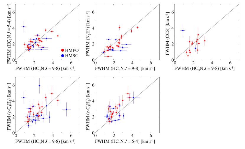
Figure 9: Relationship of FWHM among observed molecular lines. The black lines indicate the FWHM (species a) = FWHM (species b). The error bars show the standard deviation.

5.2 A Possible Chemical Evolutionary Indicator, $N$(N₂H⁺)/$N$(HC₃N)

In this paper, we test the $N$(N₂H⁺)/$N$(HC₃N) column density ratio for a chemical evolutionary indicator in high-mass star-forming regions, motivated by Suzuki et al. (1992) and Hirota et al. (2009). The different source distances and/or different source sizes could cause uncertainties in the column density estimate. The column density ratios, however, are robust, if we assume that the spatial distributions of each species are similar in all the sources. Since HC₃N is known as an early-type carbon-chain species in low-mass star-forming regions (e.g., Suzuki et al., 1992) and detected from almost all of the sources, we choose HC₃N as an early-type species. We select N₂H⁺ as a late-type species because it has confirmed in low-mass star-forming regions (Benson et al., 1998). In addition, we can avoid significant beam dilution and contamination from other sources as far as possible; N₂H⁺ can be observed with a smaller beam size compared to NH₃, e.g., the ($J,K$) = (1,1) inversion transition in the 23 GHz band is observed with the beam size of $\sim 80\arcsec$ with the Nobeyama 45-m telescope. Both HC₃N and N₂H⁺ seem to trace similar regions (dense core parts) as discussed in Section 5.1. Therefore, we will study the chemical evolution of massive cores, using the $N$(N₂H⁺)/$N$(HC₃N) ratio. Although we use different molecules from Suzuki et al. (1992) and Hirota et al. (2009), N₂H⁺ and HC₃N have been known as a late-type species and an early-type species in low-mass star-forming regions, as mentioned in Section 1. Therefore, we expect that the $N$(N₂H⁺)/$N$(HC₃N) ratio increases from HMSCs to HMPOs, if the ratio in high-mass star-forming regions similarly changes.

Figure 10 shows the relationship between the $N$(N₂H⁺)/$N$(HC₃N) ratio and $N$(HC₃N) in high-mass star-forming regions. We checked the 1.2 mm continuum images of target sources (Beuther et al., 2002; Sridharan et al., 2005) and found that several IRAS observed positions were not at exact continuum peak positions, but the beam covered the continuum core in the beam edge. We plot such data points as “Off-HMPO” in Figure 10. In some HMSCs, saturated COMs (CH₃OH and CH₃CN) and/or SiO were detected (Beuther & Sridharan, 2007). These molecular emission lines indicate star formation activity (Beuther & Sridharan, 2007). We plot these HMSCs as “HMSC associated with hot core species and/or SiO”.

Figure 10 shows that the $N$(N₂H⁺)/$N$(HC₃N) ratio tends to decrease from HMSCs to HMPOs and the $N$(HC₃N) value increases. As we mentioned in Section 1, the $N$(nitrogen-bearing molecules)/$N$(carbon-chain molecules) ratio increases from starless cores to star-forming cores in low-mass star-forming regions. Hence, this tendency in high-mass star-forming regions is clearly opposite to that in low-mass star-forming regions (Suzuki et al., 1992; Hirota et al., 2009).

We conducted the Kolmogorov-Smirnov (K-S) test about the $N$(N₂H⁺)/$N$(HC₃N) ratio and $N$(HC₃N). We included samples of “HMPO” and “HMSC”. We summarize the probabilities that the $N$(N₂H⁺)/$N$(HC₃N) ratios and the $N$(HC₃N) values in HMSCs and HMPOs originate from the same parent populations in Table 8. The probabilities were derived to be 0.75% and 1.54% for the $N$(N₂H⁺)/$N$(HC₃N) ratio and the $N$(HC₃N) value, respectively.

Furthermore, we conducted the Welch’s t test. The results are summarized in Table 8. The average value of the $N$(N₂H⁺)/$N$(HC₃N) ratio in HMSCs (20.4) is higher than that in HMPOs (3.7). The average value of $N$(HC₃N) in HMSCs is lower than that in HMPOs by a factor of 5. Thus, the differences in the $N$(N₂H⁺)/$N$(HC₃N) ratio and the $N$(HC₃N) value between HMSC and HMPO are reliable.

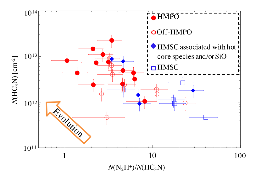
Figure 10: Relationship between $N$(N₂H⁺)/$N$(HC₃N) and $N$(HC₃N). The error bars show the standard deviation. Off-HMPO means that IRAS observed positions were not at exact continuum peak positions, but the beam covered the continuum core in the beam edge.

Table 8: Summary of statistical analyses

	$N$(N2H+)/$N$(HC3N)	$N$(HC3N)
K-S test p-value	0.75%	1.54%
Welch’s t test p-value	4.36%	0.43%
Mean (HMSC)	20.4	$1.4\times 10^{12}$ cm-2
Mean (HMPO)	3.7	$7.2\times 10^{12}$ cm-2

5.3 Explanation for the Changes in the $N$(N₂H⁺)/$N$(HC₃N) Ratio

Two possible factors can contribute to the decrease in the $N$(N₂H⁺)/$N$(HC₃N) ratio: an increase in $N$(HC₃N) and a decrease in $N$(N₂H⁺). Figure 11 shows the plot of $N$(HC₃N) vs. $N$(N₂H⁺).

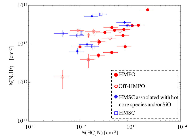
Figure 11: Relationship between $N$(N₂H⁺) and $N$(HC₃N). The error bars show the standard deviation.

Plots of N₂H⁺ in HMPOs seem to slightly below those in HMSCs. We conducted the K-S test and Welch’s t test for the N₂H⁺ column density, $N$(N₂H⁺). The probability that the $N$(N₂H⁺) values in HMSCs and HMPOs originate from the same parent populations was derived to be 77%. The average values of $N$(N₂H⁺) are $2.4\times 10^{13}$ cm^-2 and $2.3\times 10^{13}$ cm^-2 in HMSCs and HMPOs, respectively. Hence, the N₂H⁺ column density does not significantly change from HMSCs to HMPOs.

Taking the fact that the excitation temperatures of N₂H⁺ (Table 6) are lower than the rotational temperatures of HC₃N (Table 5) or NH₃ ($T_{\rm{rot}}\sim 20$ K; Sridharan et al., 2002) into consideration, N₂H⁺ seems to survive in colder parts of cores. Besides the electron recombination reactions, N₂H⁺ is destroyed by the reaction with CO molecules, which are sublimated from grain mantles with the dust temperature above 20 K (Yamamoto et al., 1983), as follows:

$${\rm{N}}_{2}{\rm{H}}^{+}+{\rm{CO}}\rightarrow{\rm{N}}_{2}+{\rm{HCO}}^{+}$$ (2)

The dust temperatures in HMPOs are much higher than 20 K ($T_{\rm{cd}}\sim 50$ K; Sridharan et al., 2002). Hence, N₂H⁺ may have been already destroyed in HMPOs at some degree, but it is not clear in our sample. This may be caused by the single-dish observation covering large linear scales. However, the reaction (2) is still one of the possible explanations for the low excitation temperatures of N₂H⁺.

As discussed in Section 5.2 and summarized in Table 8, the HC₃N column density increases from HMSCs to HMPOs. HC₃N may be formed from CH₄ (Hassel et al., 2008) and/or C₂H₂ (Chapman et al., 2009) evaporated from grain mantles in HMPOs (Taniguchi et al., 2016, 2018b). The sublimation temperatures of CH₄ and C₂H₂ are approximately 25 K and 50 K, respectively (Yamamoto et al., 1983). The dust temperatures in HMPOs are higher than these sublimation temperatures, and thus they are possible parent species of HC₃N.

We investigated the relationship between the column density and rotational temperature of HC₃N, as shown in Figure 12. We conducted the Kendall’s rank correlation statics. The probability that $N$(HC₃N) and $T_{\rm{rot}}$(HC₃N) are not related is 62.6% in HMSCs. The corresponding probability and the Kendall’s tau correlation coefficient ($\tau$) in HMPOs are 0.65% and $+0.41$, respectively. Hence, $N$(HC₃N) tends to increase with $T_{\rm{rot}}$(HC₃N) in HMPOs, whereas they are not related with each other in HMSCs. This may suggest that HC₃N is newly formed around massive young protostars.

As discussed above, the gas-phase chemical composition around massive young protostars may be affected by the molecules evaporated from grain mantles; CO, CH₄, and/or C₂H₂. This could bring the difference between high-mass star-forming regions and low-mass star-forming regions. The dust temperatures around massive young protostars are higher than those around low-mass protostars and the wider area should be heated by massive young protostars. In such a condition in high-mass star-forming regions, more molecules are sublimated from grain mantles in wider regions and the sublimated species may have more significant effects on the gas-phase chemical reactions.

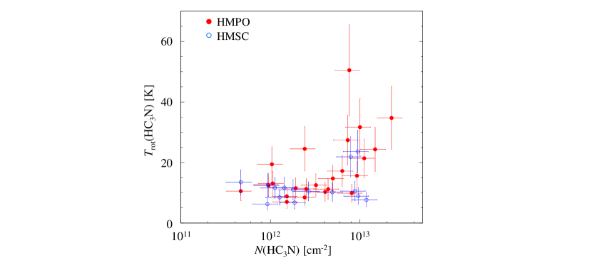
Figure 12: Relationship between rotational temperature and column density of HC₃N. The error bars show the standard deviation.

5.4 Comparisons of Detection Rates of Carbon-Chain Species with Previous Studies

As we mentioned before (Section 3), this dataset is the deepest survey observations of carbon-chain molecules in high-mass star-forming regions. We then discuss including weak molecular emission lines in this subsection.

The detection rates of HC₃N, $c$-C₃H₂, and CCS are 93, 68, and 46%, respectively, in HMPOs, including tentative detection. Taniguchi et al. (2018b) reported that the detection rate of HC₅N is 50% in HMPOs.

Law et al. (2018) carried out observations toward 16 deeply embedded (Class 0/I) low-mass protostars using the IRAM 30-m telescope. They reported that the detection rates of CCS, CCCS, HC₃N, HC₅N, $l$-C₃H, and C₄H are 88%, 38%, 75%, 31%, 81%, and 88%, respectively.

We found that the detection rates of carbon-chain molecules are probably different between high-mass protostars and low-mass protostars. In our sample, HC₃N has been detected in almost all of our target HMPOs, but HC₅N and CCS have been detected in approximately half of sample. On the other hand, CCS is most frequently detected and HC₅N shows the lowest detection rate around low-mass protostars. The low detection rate of HC₅N around low-mass protostars may be caused by observed transitions; Law et al. (2018) observed HC₅N using the high-excitation-energy lines ($E_{\rm{u}}/k>80.5$ K), while Taniguchi et al. (2018b) observed its $J=16-15$ line ($E_{\rm{u}}/k=17.4$ K). However, the results that HC₃N is more commonly detected around high-mass protostars are plausible.

Some differences between chemistry of cyanopolyynes and CCS may cause the different detection rates between high-mass star-forming regions and low-mass star-forming regions. For example, cyanopolyynes and $c$-C₃H₂ do not react with atomic oxygen in the gas phase, whereas CCS reacts with oxygen atoms to produce CO and CS. Some possibilities for the abundant atomic oxygen in high-mass star-forming regions could be considered:

• Atomic oxygen is efficiently evaporated from grain mantles with the dust temperature above $\sim 60$ K (e.g., Furuya et al., 2013).

• Strong UV radiation destroys CO molecules and the abundance of atomic oxygen may be high around HMPOs, compared to around low-mass protostars (Jørgensen et al., 2006; Goicoechea et al., 2016).

• Cosmic rays may contribute to the formation of atomic oxygen via the following reactions (e.g., Fontani et al., 2017):

  $${\rm{He}}^{+}+{\rm{CO}}\rightarrow{\rm{O}}+{\rm{C}}^{+}+{\rm{He}}.$$ (3)

The second and third ones heavily depend on physical conditions, especially the density structures, and we cannot conclude that they have large impacts. On the other hand, the first one is the most important origin when the dust temperature is above 60 K, according to the gas-grain-bulk three-phase chemical network simulation (Taniguchi et al., in prep.). The dust temperatures in HMPOs are higher than 60 K (Sridharan et al., 2002), and then atomic oxygen can be evaporated from dust grains. CCS may be efficiently destroyed around HMPOs by the reaction with atomic oxygen and the detection rate decreases.

Further observations and chemical network simulations are necessary for explanations for differences in carbon-chain chemistry between high-mass protostars and low-mass protostars.

6 Conclusions

We have carried out survey observations of molecular lines of HC₃N, N₂H⁺, $c$-C₃H₂, and CCS in the 81$-$94 GHz band toward 17 HMSCs and 28 HMPOs with the Nobeyama 45-m radio telescope. We achieved the deepest survey observations of carbon-chain species in high-mass star-forming regions.

We investigate the $N$(N₂H⁺)/$N$(HC₃N) ratio as a chemical evolutionary indicator in high-mass star-forming regions. The $N$(N₂H⁺)/$N$(HC₃N) ratio decreases from HMSCs to HMPOs, which is an opposite result to low-mass star-forming regions. From the statistical analyses, we confirmed that the HC₃N column density increases from HMSCs to HMPOs, whereas that of N₂H⁺ does not significantly change. In addition, the excitation temperatures of N₂H⁺ are lower than the rotational temperatures of HC₃N and NH₃ in both HMSCs and HMPOs. This implies that N₂H⁺ exists in cold dense cores, where the CO molecules do not sublimate from grain mantles. On the other hand, HC₃N may be newly formed from CH₄ and/or C₂H₂ evaporated from grain mantles in the warm gas around massive young protostars. This seems to be supported by the correlation between the rotational temperature and column density of HC₃N in HMPOs.

We compare the detection rates of carbon-chain species between high-mass protostars and low-mass protostars. In high-mass protostars, the detection rates of cyanopolyynes are higher compared to low-mass protostars, while the detection rate of CCS is significantly low in high-mass protostars. We discuss one possible interpretation involving atomic oxygen for the different carbon-chain detection rates between high-mass protostars and low-mass protostars. Additional observations and chemical network simulations are necessary.

Appendix A Rotational Diagram Fitting of HC₃N

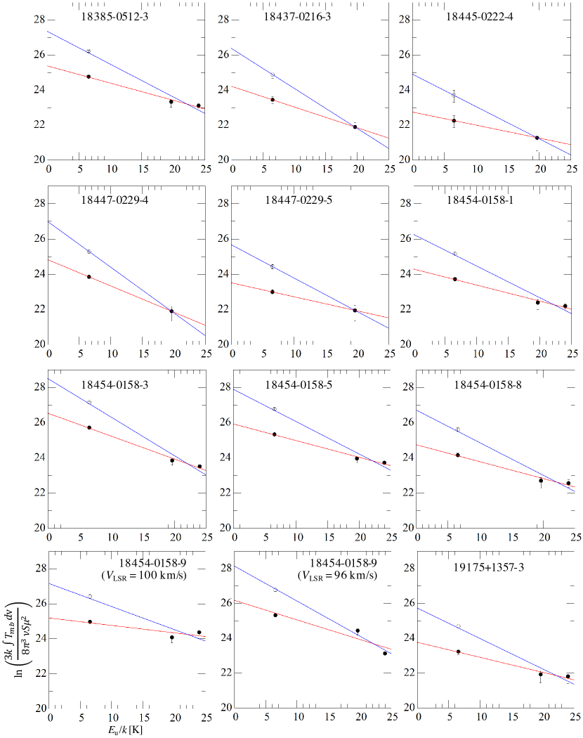
Figure 13: Rotational diagram of HC₃N. Open circle and filled circle of $J=5-4$ transition represent values with and without beam size correction, respectively. Blue and red lines indicate fitting results for with and without beam size correction, respectively. The errors were derived from the Gaussian fitting of spectra.

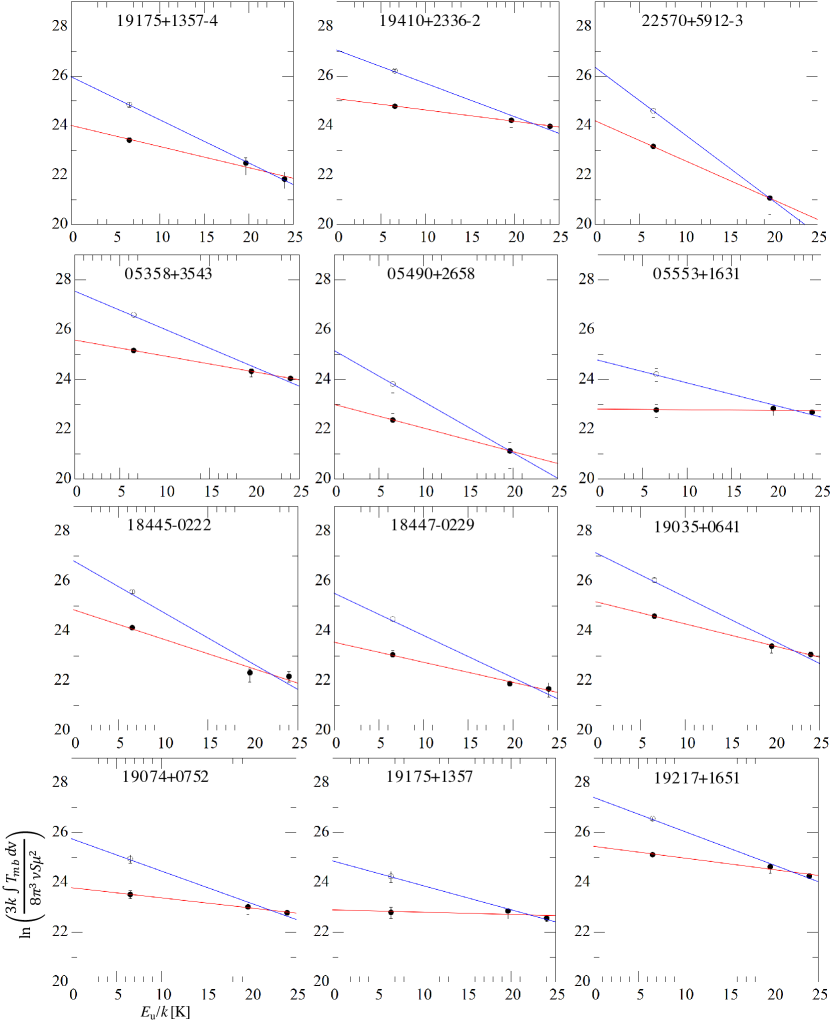
Figure 14: Continue.

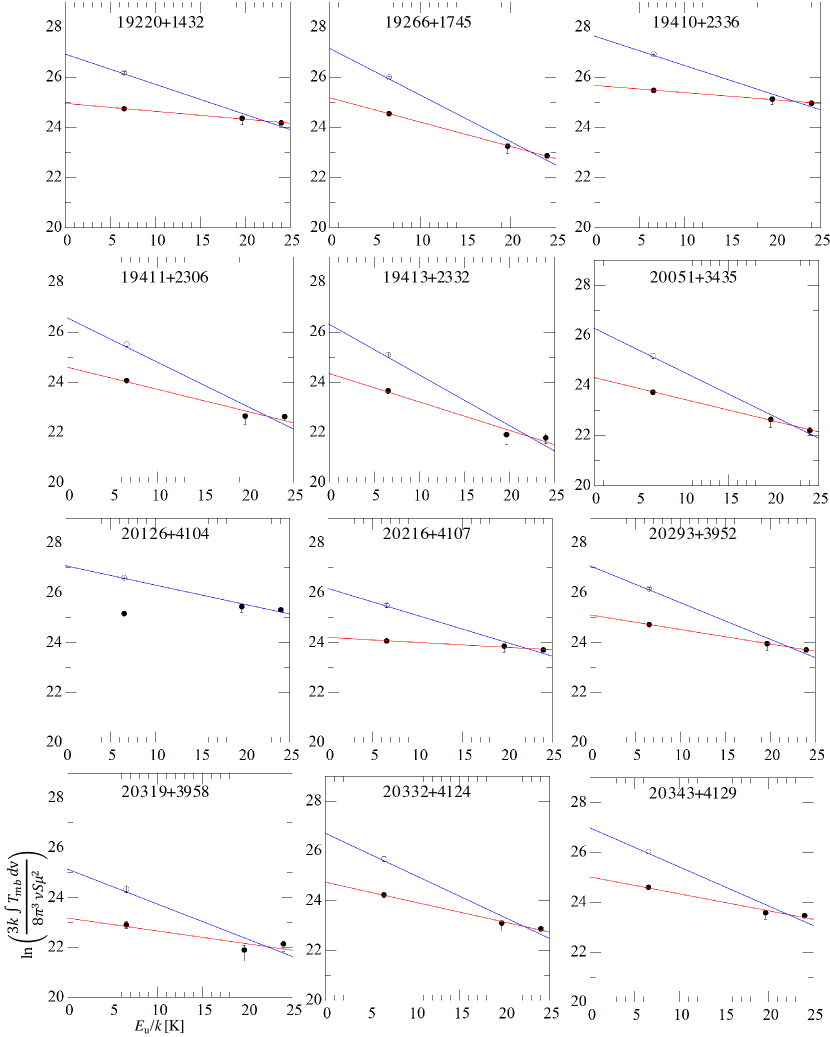
Figure 15: Continue.

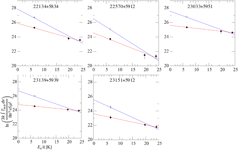
Figure 16: Continue.

References

- Adams (2010) Adams, F. C. 2010, ARA&A, 48, 47
- Benson et al. (1998) Benson, P. J., Caselli, P., & Myers, P. C. 1998, ApJ, 506, 743
- Beuther et al. (2002) Beuther, H., Schilke, P., Menten, K. M., et al. 2002, ApJ, 566, 945
- Beuther & Sridharan (2007) Beuther, H., & Sridharan, T. K. 2007, ApJ, 668, 348
- Caselli & Ceccarelli (2012) Caselli, P., & Ceccarelli, C. 2012, A&A Rev., 20, 56
- Chapman et al. (2009) Chapman, J. F., Millar, T. J., Wardle, M., Burton, M. G., & Walsh, A. J. 2009, MNRAS, 394, 221
- Deleon & Muenter (1985) Deleon, R. L., & Muenter, J. S. 1985, JChPh, 82, 1702
- Dobashi et al. (2005) Dobashi, K., Uehara, H., Kandori, R., et al. 2005, PASJ, 57, S1
- Fontani et al. (2017) Fontani, F., Ceccarelli, C., Favre, C., et al. 2017, A&A, 605, A57
- Foster et al. (2011) Foster, J. B., Jackson, J. M., Barnes, P. J., et al. 2011, ApJS, 197, 25
- Furuya et al. (2013) Furuya, K., Aikawa, Y., Nomura, H., Hersant, F., & Wakelam, V. 2013, ApJ, 779, 11
- Furuya et al. (2006) Furuya, R. S., Kitamura, Y., & Shinnaga, H. 2006, ApJ, 653, 1369
- Goicoechea et al. (2016) Goicoechea, J. R., Pety, J., Cuadrado, S., et al. 2016, Nature, 537, 207
- Goldsmith & Langer (1999) Goldsmith, P. F., & Langer, W. D. 1999, ApJ, 517, 209
- Hassel et al. (2008) Hassel, G. E., Herbst, E., & Garrod, R. T. 2008, ApJ, 681, 1385
- Hirota et al. (2009) Hirota, T., Ohishi, M., & Yamamoto, S. 2009, ApJ, 699, 585
- Hoq et al. (2013) Hoq, S., Jackson, J. M., Foster, J. B., et al. 2013, ApJ, 777, 157
- Jackson et al. (2013) Jackson, J. M., Rathborne, J. M., Foster, J. B., et al. 2013, PASA, 30, e057
- Jørgensen et al. (2006) Jørgensen, J. K., Johnstone, D., van Dishoeck, E. F., & Doty, S. D. 2006, A&A, 449, 609
- Kuiper et al. (1996) Kuiper, T. B. H., Langer, W. D., & Velusamy, T. 1996, ApJ, 468, 761
- Law et al. (2018) Law, C. J., Öberg, K. I., Bergner, J. B., & Graninger, D. 2018, ApJ, 863, 88
- Mangum & Shirley (2015) Mangum, J. G., & Shirley, Y. L. 2015, PASP, 127, 266
- Müller et al. (2005) Müller, H. S. P., Schlöder, F., Stutzki, J., & Winnewisser, G. 2005, Journal of Molecular Structure, 742, 215
- Rathborne et al. (2016) Rathborne, J. M., Whitaker, J. S., Jackson, J. M., et al. 2016, PASA, 33, e030
- Sakai et al. (2008) Sakai, T., Sakai, N., Kamegai, K., et al. 2008, ApJ, 678, 1049
- Suzuki et al. (1992) Suzuki, H., Yamamoto, S., Ohishi, M., et al. 1992, ApJ, 392, 551
- Sridharan et al. (2005) Sridharan, T. K., Beuther, H., Saito, M., Wyrowski, F., & Schilke, P. 2005, ApJ, 634, L57
- Sridharan et al. (2002) Sridharan, T. K., Beuther, H., Schilke, P., Menten, K. M., & Wyrowski, F. 2002, ApJ, 566, 931
- Takakuwa et al. (2001) Takakuwa, S., Kawaguchi, K., Mikami, H., & Saito, M. 2001, PASJ, 53, 251
- Taniguchi et al. (2016) Taniguchi, K., Saito, M., & Ozeki, H. 2016, ApJ, 830, 106
- Taniguchi et al. (2018a) Taniguchi, K., Saito, M., Majumdar, L., et al. 2018a, ApJ, 866, 150
- Taniguchi et al. (2018b) Taniguchi, K., Saito, M., Sridharan, T. K., & Minamidani, T. 2018b, ApJ, 854, 133
- Tatematsu et al. (2017) Tatematsu, K., Liu, T., Ohashi, S., et al. 2017, ApJS, 228, 12
- Yamamoto (2017) Yamamoto, S. 2017, Introduction to Astrochemistry: Chemical Evolution from Interstellar Clouds to Star and Planet Formation, Astronomy and Astrophysics Library, by Satoshi Yamamoto. ISBN 978-4-431-54170-7. Springer Japan, 2017
- Yamamoto et al. (1983) Yamamoto, T., Nakagawa, N., & Fukui, Y. 1983, A&A, 122, 171
- Yu & Wang (2015) Yu, N., & Wang, J.-J. 2015, MNRAS, 451, 2507