Slim LSTM NETWORKS: LSTM_6 and LSTM_C6

Abstract

We have shown previously that our parameter-reduced variants of Long Short-Term Memory (LSTM) Recurrent Neural Networks (RNN) are comparable in performance to the standard LSTM RNN on the MNIST dataset. In this study, we show that this is also the case for two diverse benchmark datasets, namely, the review sentiment IMDB and the 20 Newsgroup datasets. Specifically, we focus on two of the simplest variants, namely LSTM_6 (i.e., standard LSTM with three constant fixed gates) and LSTM_C6 (i.e., LSTM_6 with further reduced cell body input block). We demonstrate that these two aggressively reduced-parameter variants are competitive with the standard LSTM when hyper-parameters, e.g., learning parameter, number of hidden units and gate constants are set properly. These architectures enable speeding up training computations and hence, these networks would be more suitable for online training and inference onto portable devices with relatively limited computational resources.

1 Introduction

Recurrent Neural Networks (RNNs) have been making an impact in sequence-to-sequence mappings, with particularly successful applications in speech recognition, music, language translation, and natural language processing to name a few [11, 22, 7, 5, 13]. By their structure, they possess a memory (or state) and include feedback or recurrence. The simple RNN (sRNN) is succinctly expressed, see e.g., [10]:

$$\begin{split}&h_{t}=\sigma(W_{hx}x_{t}+W_{hh}h_{t-1}+b_{h})\\ &y_{t}=W_{hy}h_{t}+b_{y}\end{split}$$ (1)

where $x_{t}$ is the input sequence vector at (time) step $t$, $h_{t}$ is the hidden (activation) unit vector at step $t$, while $h_{t-1}$ is the hidden unit vector at the previous step $t-1$, and $y_{t}$ is the output vector at step $t$. The parameters are the three matrices, namely, $W_{hx},W_{hh}$, and $W_{hy}$, and the vector $b_{h}$. This constitutes a discrete-step dynamic recurrent system with $h_{t}$ acting as the state. The parameters are to be determined adaptively via training mostly using various versions of backpropagation through time (BPTT), e.g., see [11].

The LSTM RNNs introduce a cell-memory and 3 gating signals to enable effective learning via the BPTT [11]. The simple activation state has been replaced with a more involved activation with gating mechanisms. The LSTM RNN uses a (additional) memory cell (vector and includes three gates: (i) an input gate, $i_{t}$ (ii) an output gate $o_{t}$, and (iii) a forget gate, $f_{t}$. These gates collectively control signaling. The standard LSTM is expressed mathematically as [11, 10]:

$$\begin{split}&i_{t}=\sigma_{in}(W_{i}x_{t}+U_{i}h_{t-1}+b_{i})\\ &f_{t}=\sigma_{in}(W_{f}x_{t}+U_{f}h_{t-1}+b_{f})\\ &o_{t}=\sigma_{in}(W_{o}x_{t}+U_{o}h_{t-1}+b_{o})\\ &\tilde{c_{t}}=\sigma(W_{c}x_{t}+U_{c}h_{t-1}+b_{c})\\ &c_{t}=f_{t}\odot c_{t-1}+i_{t}\odot\tilde{c_{t}}\\ &h_{t}=o_{t}\odot\sigma(c_{t})\end{split}$$ (2)

where the first 4 equations are replica of the simple RNN (sRNN) above, with the first 3 equations serving as gating signals and thus their nonlinear activation is set as a sigmoid function $\sigma_{in}$, while the 4th equation’s nonlinearity is an arbitrary nonlinearity $\sigma$, typically sigmoid, hyperbolic tangent ($tanh$), or rectified linear unit (reLU). This 4th equation is sometimes referred to as the input block. The last two equations entail the memory cell $c_{t}$ and now activation hidden unit $h_{t}$ with the insertion of the gating signals ina point-wise (Haramard) multiplications (using the symbol $\odot$). This represents a discrete-step nonlinear dynamic system with recurrence. The distinct parameters are associated with each replica as $W_{*},U_{*}$, and $b_{*}$ is a straight fashion.

The output layer of the LSTM model may be chosen to be as a linear (more accurately, affine) map as

$$y_{t}=W_{hy}h_{t}+b_{y}$$ (3)

where $y_{t}$ is the output, and $W_{hy}$ is a matrix, and $b_{y}$ is a bias vector. In other optional implementation, this layer may be followed by a softmax layer to render the output analogous with probability ranges.

LSTMs are relatively compationally expensive due to the fact that they have four replica with distinct sets of parameters (namely, weights and biases) which would need to be adaptively updated every (mini-batch) of training calculations.

We have introduced numerous, computationally simpler, LSTM variants by aggressively eleminating some of the adaptive parameters, see [20, 16, 1, 2, 3, 21, 14]. In this study we shall focus on one of the simplest variant forms, namely the slim LSTM_6 and LSTM_C6 [21, 2].

2 LSTM_6

Different variants have been introduced earlier [3, 21]. For LSTM_6, the gating signals are set at constant values as follows:

$$\begin{split}&i_{t}=1.0\\ &f_{t}=f,~{}-1<f<1.0\\ &o_{t}=1.0\\ &\tilde{c_{t}}=\sigma(W_{c}x_{t}+U_{c}h_{t-1}+b_{c})\\ &c_{t}=f_{t}\odot c_{t-1}+i_{t}\odot\tilde{c_{t}}\\ &h_{t}=o_{t}\odot\sigma(c_{t})\end{split}$$ (4)

Note that the gate signal values are set to the constant scalars $f$ or $1$. In practice, when the gate is set to $1$, it is equivalent to eliminating the gate entirely! Thus, in compact form, the LSTM_6 equation now reads:

$$\begin{split}&c_{t}=f~{}c_{t-1}+\sigma(W_{c}x_{t}+U_{c}h_{t-1}+b_{c}),~{}~{}-1<f<1.0\\ &h_{t}=\sigma(c_{t})\end{split}$$ (5)

This variant form is close to the so-called basic Recurrent Neural Network (bRNN), see [19, 21] for analysis and details.

3 LSTM_C6

In LSTM_C6 the matrix $U_{c}$ in the cell equation is replaced with a corresponding vector $u_{c}$, in order to render a point-wise multiplication instead. This the variant equations become

$$\begin{split}&i_{t}=1.0\\ &f_{t}=f,~{}-1<f<1.0\\ &o_{t}=1.0\\ &\tilde{c_{t}}=\sigma(W_{c}x_{t}+u_{c}\odot h_{t-1}+b_{c})\\ &c_{t}=f_{t}\odot c_{t-1}+i_{t}\odot\tilde{c_{t}}\\ &h_{t}=o_{t}\odot\sigma(c_{t})\end{split}$$ (6)

Similarly, in compact form, these equations now read as:

$$\begin{split}&c_{t}=f~{}c_{t-1}+\sigma(W_{c}x_{t}+u_{c}\odot h_{t-1}+b_{c}),~{}~{}-1<f<1.0\\ &h_{t}=\sigma(c_{t})\end{split}$$ (7)

To account for the number of parameters in each case, let the input vector $x_{t}$ be of $m$ dimension, the state $c_{t}$ and its activation hidden unit has dimension of $n$. Then the number of (adaptive) parameters in LSTM_6 is $n(m+n+1)$ and for LSTM_C6 the total number of (adaptive) parameters is $n(m+2)$. (Note that one may add to each the new nonadaptive hyper-parameter $f$). Thus if the state dimension $n=100$ and the input dimension is $m=32$, the total number of (adaptive) parameters for LSTM_6 is $3400$.

Table I and Table II provide a summary of the number of parameters as well as the times per epoch during training corresponding to each of the model variants for $h=100$ for each data set. The number of parameter only include parameter corresponding to LSTM layer and parameter of embedding and last dense layer is not included. These simulation and the training times are obtained by running the Keras Library [6] with GPU option enable. Although, we expect that LSTM_C6 takes less time per epoch than LSTM6, but due to Keras internal implementation, that is not the case. However, LSTM_C6 is still faster than basic LSTM. Comparing these two table indicate that time-wise, parameter reduction plays a huge role in larger networks.

TABLE I: Variants specifications: IMDB Dataset

variants	# of parameters	dimensions
LSTM	53200	m=32, n=100
LSTM6	13300	m=32, n=100
LSTM_C6	3400	m=32, n=100

TABLE II: Variants specifications: 20 Newsgroup Dataset

variants	# of parameters	dimensions
LSTM	263168	m=128, n=128
LSTM6	65792	m=128, n=128
LSTM_C6	33280	m=128, n=128

4 Experiments and Discussion

In the previous work [2], we have shown that our networks are competitively comparable to standard LSTM networks on the MNIST dataset. Here we show that LSTM_6 (also denoted here as LSTM6) and LSTM_C6 can compete with the standard LSTM network in the benchmark public datasets IMDB and 20 Newsgroup available via the Keras library https://keras.io.

4.1 The IMDB dataset

IMDB Datasets is a binary sentiment classification dataset. To train the model, dictionary size of 5000 has been used. Each review is truncated or padded to 500 words. The first layer is an embedding layer which is a simple multiplication that transforms words into their corresponding word embedding. The output is then passed to an LSTM layer following a dense layer. The network specification which has been adopted from Keras 1.2 examples is given in table III.

TABLE III: Network specifications: IMDB Datasets

Input dimension	$500\times 32$
Number of hidden units	$100,200,300,400$
Non-linear function	sigmoid
Output dimension	1
Number of epochs	$100$
Optimizer	Adam
Batch size	$32$
Loss function	binary cross-entropy

A schematic representation of the architecture used is given in figure 1.

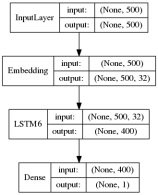
Figure 1: Network Architecture Diagram for IMDB

In this experiment, the $sigmoid$ nonlinearity is used, since the $tanh$ nonlinearity has caused large fluctuations in training and testing outcomes and using the $reLU$ nonlinearity routinely failed to converge even for the standard LSTM RNN.

4.1.1 Tuning the hyper-parameter $\eta$

We started with the generic $\eta=1\mathrm{e}{-3}$ as used in the Keras library example. As it is shown in figure 2, the standard LSTM (denoted as lstm0 in the figure) displays smooth profiles with (testing) accuracy around $88\%$. However, LSTM_6 (denoted as LSTM6 in the figure) shows fluctuations and also does not catch up with standard LSTM. This is an indicator that $\eta=1\mathrm{e}{-3}$ is too large for this variant network. Since the number of parameters in LSTM6 has aggressively been reduced, it is expected that the different optimal values of $\eta$ would work better. This is study, we consider a grid of two values around the default value. Decreasing $\eta$ to $1e-4$ improves the performance of LSTM6 to $82\%$ , however a small amount of fluctuation is still observed. Meanwhile, LSTM_C6 did not show any improvement.

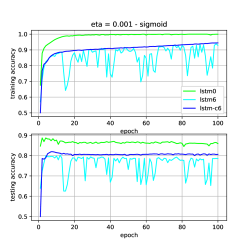
Figure 2: IMDB, Training & Test accuracy, $\sigma=sigmoid,\eta=1\mathrm{e}{-3}$

Figure 3: IMDB, Training & Test accuracy, $\sigma=sigmoid,\eta=1\mathrm{e}{-4}$

The typical results obtained over the eta-grid among all the epochs are shown in Table IV.

TABLE IV: Best results obtained for IMDB using sigmoid

		$\eta=1\mathrm{e}{-4}$	$\eta=1\mathrm{e}{-3}$	$\eta=2\mathrm{e}{-3}$
LSTM	train	0.9906	1.0000	0.9600
	test	0.8856	0.8868	0.7775
LSTM6	train	0.9489	0.9387	0.7850
	test	0.8208	0.8026	0.7100
LSTM_C6	train	0.8992	0.9445	0.9556
	test	0.8174	0.8192	0.7842

4.1.2 Increasing the dimension of the state or hidden units

To compensate for decreased number of parameters, the dimension of hidden units has been increased along with different smaller values of $\eta$. As it is shown, higher dimensions need less epoch to reach leveling off profiles. Setting $\eta=1.25e-5$, creates an almost fluctuation free profile. In the following figures lstm62 stands for LSTM6 using 200 hidden units.

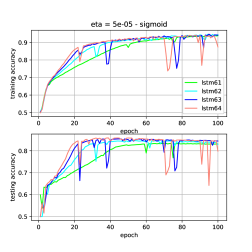
Figure 4: IMDB, Training & Test accuracy, $\sigma=sigmoid,\eta=5\mathrm{e}{-5}$

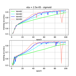
Figure 5: IMDB, Training & Test accuracy, $\sigma=sigmoid,\eta=2.5\mathrm{e}{-5}$

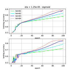
Figure 6: IMDB, Training & Test accuracy, $\sigma=sigmoid,\eta=1.25\mathrm{e}{-5}$

TABLE V: Best results obtained Using sigmoid.

		$\eta=5\mathrm{e}{-5}$	$\eta=2.5\mathrm{e}{-5}$	$\eta=1.25\mathrm{e}{-5}$
100	train	0.9396	0.8871	0.7783
	test	0.8340	0.8206	0.7219
200	train	0.9461	0.9185	0.833
	test	0.8461	0.8459	0.7908
300	train	0.9471	0.9319	0.8754
	test	0.8542	0.8567	0.8374
400	train	0.9404	0.933	0.8887
	test	0.8585	0.8618	0.8523

4.1.3 Tuning the constant forget hyper-paramter

The forget (gate) constant value must be less than one in absolute value for bounded-input-bounded-output (BIBO) stability [19]. In our previous work [3], $f~{}>~{}0.59$ did not work for the MNIST dataset and training would not converge. In this paper on this different dataset, we initially start with the same value (i.e., $f~{}=~{}0.59$ . To fill in the gap between standard LSTM and LSTM6, we gradually increase the forget hyperparamter $f$ and observe that IMDB dataset produce BIBO stable performance up to $f_{t}=0.96$. Since the accurcy plot profiles show increasing performance trend and do not appear to level off after $100$ epochs. We run the training for $200$ epochs. It is observed that LSTM6 surpass standard LSTM at around epoch $150$.

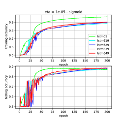
Figure 7: IMDB, Training & Test accuracy, $\sigma=sigmoid,\eta=1\mathrm{e}{-5}$

The effect of increasing the hyper-parameter $f$ in the LSTM_C6 network using $h=200$ and $\eta=\mathrm{e}{-5}$ is also depicted in figure 8. In this figure, lstm-c6295 denotes LSTM_C6 using $h=200$ and $f=0.95$.

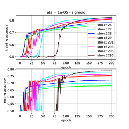
Figure 8: IMDB, Training & Test accuracy, $\sigma=sigmoid,\eta=1\mathrm{e}{-5}$

4.2 The20 Newsgroups dataset

The 20 Newsgroups dataset is a collection of 20000 documents, containing 20 different newsgroups. GloVe embedding is used to pre-train the model [6]. The network architecture is adapted from Keras1.2 examples. Table VI provides the network specification. We have applied our variants in the bidirectional layer. A schematic representation of the architecture used is given in figure 9.

TABLE VI: Network specifications.

Input dimension	$1000$
Embedding layer	$1000\times 100$
Conv1D(128, 5,’relu’)	$996\times 128$
Maxpooling1D(5)	$199\times 128$
Conv1D(128, 5,’relu’)	$195\times 128$
Maxpooling1D(5)	$39\times 128$
Conv1D(128, 5,’relu’)	$35\times 128$
Maxpooling1D(2)	$17\times 128$
Number of epochs	$100$
Bidirectional(lstmi)	256
Dense	128
Dense	6
Optimizer	rmsprop
Batch size	$128$
Loss function	categorical cross-entropy

Figure 9: News20, Network Architecture Diagram

4.2.1 The tanh activation

Using $tanh$ as nonlinearity, the LSTM_C6 layer results in better performance than using the LSTM6 layer and even using the standard LSTM layer. It is observed that setting $\eta=1\mathrm{e}{-3}$ results in test score of $79.42\%$ in LSTM_C6 which surpasses the test score of the standard LSTM, $77.75\%$, using $\eta=2\mathrm{e}{-3}$. The best results obtained for the three grid values of $eta$ over100 epochs are summarized in Table VII.

TABLE VII: Best results obtained for news20 LSTM models

		$\eta=5\mathrm{e}{-4}$	$\eta=1\mathrm{e}{-3}$	$\eta=2\mathrm{e}{-3}$
LSTM	train	0.9519	9581	0.9600
	test	0.7592	0.7750	0.7775
LSTM6	train	0.8169	0.8448	0.7850
	test	0.7158	0.7200	0.7100
LSTM_C6	train	0.9552	0.9583	0.9556
	test	0.7792	0.7942	0.7842

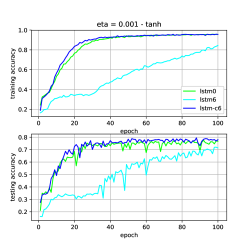
Figure 10: News20, Training & Test accuracy, $\sigma=tanh,\eta=1\mathrm{e}{-3}$

Figure 11: News20, Training & Test accuracy, $\sigma=tanh,\eta=5\mathrm{e}{-4}$

4.2.2 The (logistic) sigmoid activation

Using $sigmoid$ as nonlinearity, the similar trend is observed; LSTM_C6 shows better performance than LSTM6 and even standard LSTM.

Figure 12: Training & Test accuracy, $\sigma=sigmoid,\eta=1\mathrm{e}{-3}$

5 Conclusion

LSTM_6 and LSTM_C6, which are aggressively reduced variant of the baseline standard LSTM have been evaluated on the benchmark classical IMDB and 20 Newsgroups datasets. In these slim LSTM variants, the gates are set at constants, and effectively only the forget gate serves now as a hyper-parameter to ensure BIBO stability of the discrete dynamic recurrent neural network (RNN). LSTM_C6 further reduced the matrix $U_{c}$ in the input block equation into a vector with point-wise (Hadamard) multiplication. We tried limited grid of 3 values of the learning rate centered around a default value for the standard LSTM RNN using in the Keras Library. Moreover, the network dimension can be used as a hyper-parameter to improved the slim LSTM variants. These investigations have shown that the capacity of the slim LSTMS can match the standard LSTM while still saving computational expense. It was observed that as we increase the number of hidden units the performance improves. Finally, using the hyper-parameter $f$ in place of the forget gate $f_{t}$, the training/ testing performance can also improve, up to to the value $f=0.96$ for the IMDB dataset. This enables LSTM6 to surpass standard LSTM at around 150 epochs. In the 20 Newsgroups dataset, LSTM_C6 surpasses base LSTM without much parameter tuning. As a results we conclude that these simplified models are comparable to the standard LSTM. Thus, these slim LSTM variants may be suitably employed in applications in order to benefit from realtime speed and/or computational expense.

References

- [1] A. Akandeh and F. M. Salem. Simplified long short-term memory recurrent neural networks: part I. arXiv:1707.04619, 2017.
- [2] A. Akandeh and F. M. Salem. Simplified long short-term memory recurrent neural networks: part II. arXiv:1707.04623, 2017.
- [3] A. Akandeh and F. M. Salem. Simplified long short-term memory recurrent neural networks: part III. arXiv:1707.04626, 2017.
- [4] Y. Bengio, P. Simard, and P. Frasconi. Learning long-term dependencies with gradient descent is difficult. IEEE transactions on neural networks, 5(2):157–166, 1994.
- [5] N. Boulanger-Lewandowski, Y. Bengio, and P. Vincent. Modeling temporal dependencies in high-dimensional sequences: Application to polyphonic music generation and transcription. arXiv preprint arXiv:1206.6392, 2012.
- [6] F. Chollet. Keras github. https://github.com/fchollet/keras/blob/master/examples.
- [7] J. Chung, C. Gulcehre, K. Cho, and Y. Bengio. Empirical evaluation of gated recurrent neural networks on sequence modeling. arXiv preprint arXiv:1412.3555, 2014.
- [8] F. A. Gers, J. Schmidhuber, and F. Cummins. Learning to forget: Continual prediction with lstm. Neural computation, 12(10):2451–2471, 2000.
- [9] F. A. Gers, N. N. Schraudolph, and J. Schmidhuber. Learning precise timing with lstm recurrent networks. Journal of machine learning research, 3(Aug):115–143, 2002.
- [10] I. Goodfellow, Y. Bengio, and A. Courville. Deep Learning. MIT Press, 2016. http://www.deeplearningbook.org.
- [11] K. Greff, R. K. Srivastava, J. Koutn´ık, B. R. Steunebrink, and J. Schmidhuber. Lstm: A search space odyssey. IEEE transactions on Neural Networks and Learning Systems, 28(10):2222–2232, 2017.
- [12] S. Hochreiter and J. Schmidhuber. Long short-term memory. Neural computation, 9(8):1735–1780, 1997.
- [13] M. Johnson, M. Schuster, Q. V. Le, M. Krikun, Y. Wu, Z. Chen, N. Thorat, F. B. Viégas, M. Wattenberg, G. Corrado, M. Hughes, and J. Dean. Google’s multilingual neural machine translation system: Enabling zero-shot translation. CoRR, abs/1611.04558, 2016.
- [14] D. Kent and F. M.Salem. Performance of three slim variants of the long short-term memory (lstm) layer. arXiv preprint arXiv:1901.00525, 2019.
- [15] Y. LeCun, C. Cortes, and C. J. Burges. Mnist handwritten digit database. AT&T Labs [Online]. Available: http://yann. lecun. com/exdb/mnist, 2, 2010.
- [16] Y. Lu and F. M. Salem. Simplified gating in long short-term memory (lstm) recurrent neural networks. arXiv:1701.03441, 2017.
- [17] T. Mikolov, A. Joulin, S. Chopra, M. Mathieu, and M. Ranzato. Learning longer memory in recurrent neural networks. arXiv preprint arXiv:1412.7753, 2014.
- [18] R. Pascanu, T. Mikolov, and Y. Bengio. On the difficulty of training recurrent neural networks. ICML (3), 28:1310–1318, 2013.
- [19] F. M. Salem. A basic recurrent neural network model. arXiv preprint arXiv:1612.09022, 2016.
- [20] F. M. Salem. Reduced parameterization in gated recurrent neural networks. Technical Report 11-2016, MSU, 2016.
- [21] F. M. Salem. Slim lstms. arXiv preprint arXiv:1812.11391, 2018.
- [22] W. Zaremba. An empirical exploration of recurrent network architectures. An empirical exploration of recurrent network architectures, 2015.
- [23] W. Zaremba, I. Sutskever, and O. Vinyals. Recurrent neural network regularization. arXiv preprint arXiv:1409.2329, 2014.