aainstitutetext: Institute for Theoretical Physics Amsterdam and Delta Institute for Theoretical Physics, University of Amsterdam, Science Park 904, 1098 XH Amsterdam, The Netherlandsbbinstitutetext: Nikhef, Theory Group, Science Park 105, 1098 XG, Amsterdam, The Netherlandsccinstitutetext: Nuclear Science Division, Lawrence Berkeley National Laboratory, Berkeley, CA 94720, USA

The Jet Shape at NLL

Pedro Cal c    Felix Ringer a,b    Wouter J. Waalewijn p.cal@nikhef.nl fmringer@lbl.gov w.j.waalewijn@uva.nl
Abstract

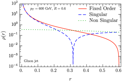
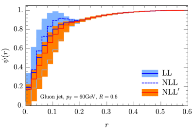
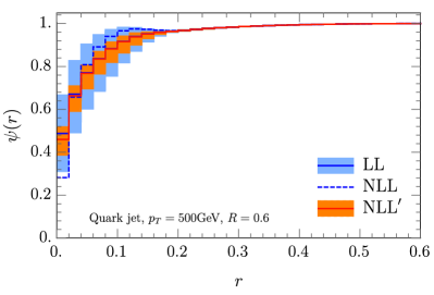
The jet shape is the fraction of the jet energy within a cone r𝑟r centered on the jet axis. We calculate the jet shape distribution at next-to-leading logarithmic accuracy plus next-to-leading order (NLL), accounting for logarithms of both the jet radius R𝑅R and the ratio r/R𝑟𝑅r/R. This is the first phenomenological study that takes the recoil of the jet axis due to soft radiation into account, which is needed to reach this accuracy, but complicates the calculation of collinear radiation and requires the treatment of rapidity logarithms and non-global logarithms. We present numerical results, finding good agreement with ATLAS and CMS measurements of the jet shape in an inclusive jet sample, ppjet+X𝑝𝑝jet𝑋pp\to{\rm jet}+X, for different kinematic bins. The effect of the underlying event and hadronization are included using a simple one-parameter model, since they are not part of our perturbative calculation.

preprint: NIKHEF 2018-035

1 Introduction

The jet shape is a classic jet substructure observable that maps out the transverse energy profile of jets Ellis:1992qq . It is one of the most frequently studied jet substructure observables, which has been measured at a variety of collider experiments over the past decades. The existing data sets include jet shape measurements in pp𝑝𝑝pp, pp¯𝑝¯𝑝p\bar{p}, ep𝑒𝑝ep, e+esuperscript𝑒superscript𝑒e^{+}e^{-} and heavy-ion collisions, and the range of different center-of-mass energies (Ecmsubscript𝐸cmE_{\rm cm}) makes the jet shape a unique testing ground for precision QCD studies. In order to achieve a meaningful comparison between the experimental data and theoretical calculations, we need to be able to make precise predictions within perturbative QCD, which is the goal of this work.

Jet shapes have been used to constrain parton shower event generators, including their models of hadronization and the underlying event contribution, see e.g. ref. ATLAS:2011gmi . Furthermore, QCD predicts that the distribution of particles in gluon jets is broader than in quark jets, making the jet shape a useful observable to discriminate between quark and gluon jets (see ref. Gras:2017jty for a recent review). More generally, jet substructure techniques have started to play an important role in the search for physics beyond the standard model Adams:2015hiv , where the separation of boosted objects from QCD jets requires a sophisticated understanding of jet substructure. For recent reviews of jet substructure techniques and their applications, see refs. Larkoski:2017jix ; Asquith:2018igt .
Refer to caption
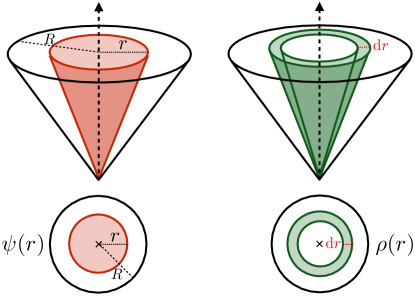
Figure 1: The integrated (differential) jet shape, shown in the left (right) panel, is the fraction of the jet transverse momentum contained in a circle (annulus) in (η,ϕ)𝜂italic-ϕ(\eta,\phi) coordinates, centered on the jet axis.

We consider inclusive jet production, ppjet+X𝑝𝑝jet𝑋pp\to{\rm jet}+X, where any observed jet in a given transverse momentum pTsubscript𝑝𝑇p_{T} and rapidity η𝜂\eta interval is taken into account, and we sum over everything else (X𝑋X) in the final state. Given such an identified jet with radius R𝑅R, the integrated jet shape ψ(r)𝜓𝑟\psi(r) and the differential jet shape ρ(r)𝜌𝑟\rho(r) are defined as follows

ψ(r)=ri<rpTiri<RpTi,ρ(r)=dψ(r)dr,formulae-sequence𝜓𝑟subscriptsubscript𝑟𝑖𝑟subscript𝑝𝑇𝑖subscriptsubscript𝑟𝑖𝑅subscript𝑝𝑇𝑖𝜌𝑟d𝜓𝑟d𝑟\psi(r)=\frac{\sum_{r_{i}<r}\,p_{Ti}}{\sum_{r_{i}<R}\,p_{Ti}}\,,\qquad\rho(r)=\frac{\mathrm{d}\psi(r)}{\mathrm{d}r}\,, (1)

see fig. 1. Here risubscript𝑟𝑖r_{i} denotes the distance in the (η,ϕ)𝜂italic-ϕ(\eta,\phi) plane of particle i𝑖i in the jet to the jet axis, and pTisubscript𝑝𝑇𝑖p_{Ti} is its transverse momentum with respect to the beam axis. The dependence on the pTsubscript𝑝𝑇p_{T}, η𝜂\eta and radius R𝑅R of the observed jet is left implicit. The integrated jet shape is normalized by construction, i.e. ψ(R)=1𝜓𝑅1\psi(R)=1. Note that it is important for the jet shape which jet axis is chosen. We will focus on the standard jet axis, which is consistent with the currently existing data sets. For a discussion of the jet shape using the winner-take-all axis Bertolini:2013iqa , see refs. Kang:2017mda ; Neill:2018wtk .

The first jet shape measurements were already performed by the OPAL collaboration at LEP Akers:1994wj . It has also been measured at the Tevatron Abe:1992wv ; Abachi:1995zw ; Acosta:2005ix , and at HERA in both deep inelastic scattering Aid:1995ma ; Adloff:1997gq ; Adloff:1998ni ; Breitweg:1998gf and photoproduction Breitweg:1997gg . At the LHC, jet shape measurements on an inclusive jet sample were performed by ATLAS Aad:2011kq and CMS Chatrchyan:2012mec at Ecm=subscript𝐸cmabsentE_{\rm cm}= 7 TeV. The jet shape has also been measured for heavy-flavor jets Aaltonen:2008de ; Aad:2013fba . We leave an extensive comparison to all these data sets for future work, focussing only on the LHC data in this paper. In recent years, jet shapes have also received a growing attention in heavy-ion collisions as a probe of the properties of the quark-gluon plasma. The transverse energy profile of jets that traverse the hot and dense QCD medium gets modified in comparison to jets in pp𝑝𝑝pp collisions. See refs. Chatrchyan:2013kwa ; CMS:2018ogb for recent experimental results from the LHC.

In this work we build upon the framework for jet shapes developed by some of us in the context of subjet distributions Kang:2017mda , and extend it to full next-to-leading logarithmic (NLL) accuracy. We employ Soft Collinear Effective Theory (SCET) Bauer:2000ew ; Bauer:2000yr ; Bauer:2001ct ; Bauer:2001yt ; Beneke:2002ph in order to achieve the resummation of lnR𝑅\ln R and ln(r/R)𝑟𝑅\ln(r/R). The starting point is our factorization of the cross section differential in jet transverse momentum pTsubscript𝑝𝑇p_{T}, rapidity η𝜂\eta, and the energy fraction zrsubscript𝑧𝑟z_{r} contained in a subjet of radius r𝑟r centered along the jet axis,

dσdpTdηdzr=a,b,cfa(xa,μ)fb(xb,μ)abc(xa,xb,η,pT/z,μ)𝒢cjet(z,zr,pTR,r/R,μ).d𝜎dsubscript𝑝𝑇d𝜂dsubscript𝑧𝑟subscript𝑎𝑏𝑐tensor-producttensor-producttensor-productsubscript𝑓𝑎subscript𝑥𝑎𝜇subscript𝑓𝑏subscript𝑥𝑏𝜇superscriptsubscript𝑎𝑏𝑐subscript𝑥𝑎subscript𝑥𝑏𝜂subscript𝑝𝑇𝑧𝜇superscriptsubscript𝒢𝑐jet𝑧subscript𝑧𝑟subscript𝑝𝑇𝑅𝑟𝑅𝜇\frac{\mathrm{d}\sigma}{\mathrm{d}p_{T}\,\mathrm{d}\eta\,\mathrm{d}z_{r}}=\sum_{a,b,c}f_{a}(x_{a},\mu)\otimes f_{b}(x_{b},\mu)\otimes{\cal H}_{ab}^{c}\left(x_{a},x_{b},\eta,p_{T}/z,\mu\right)\otimes{\mathcal{G}}_{c}^{\rm jet}(z,z_{r},p_{T}R,r/R,\mu)\,. (2)

Here fa,bsubscript𝑓𝑎𝑏f_{a,b} denote the PDFs for the incoming protons, the hard functions abcsuperscriptsubscript𝑎𝑏𝑐{\cal H}_{ab}^{c} describe the hard scattering abc+X𝑎𝑏𝑐𝑋ab\to c+X and tensor-product\otimes denote appropriate integrals over the momentum fractions xa,bsubscript𝑥𝑎𝑏x_{a,b} and z𝑧z (see eq. (2.1) for more details). The production of the jet, including the measurement of the energy fraction zrsubscript𝑧𝑟z_{r}, is captured by the jet function 𝒢cjetsuperscriptsubscript𝒢𝑐jet{\mathcal{G}}_{c}^{\rm jet}. The factorization in eq. (2) holds for narrow jets and is analogous to inclusive hadron production, with fragmentation functions replaced by jet functions Kaufmann:2015hma ; Kang:2016mcy ; Dai:2016hzf . The integrated jet shape ψ(r)𝜓𝑟\psi(r) in eq. (1) is then given by the energy average of the zrsubscript𝑧𝑟z_{r} differential cross section normalized by the inclusive jet cross section

ψ(r)=01𝑑zrzrdσdpTdηdzr/dσdpTdη.𝜓𝑟superscriptsubscript01differential-dsubscript𝑧𝑟subscript𝑧𝑟d𝜎dsubscript𝑝𝑇d𝜂dsubscript𝑧𝑟d𝜎dsubscript𝑝𝑇d𝜂\psi(r)=\int_{0}^{1}dz_{r}\,z_{r}\frac{\mathrm{d}\sigma}{\mathrm{d}p_{T}\,\mathrm{d}\eta\,\mathrm{d}z_{r}}\,\Big{/}\,\frac{\mathrm{d}\sigma}{\mathrm{d}p_{T}\,\mathrm{d}\eta}\,. (3)

The expression for ψ(r)𝜓𝑟\psi(r) involves single logarithms in the jet radius parameter αsnlnnRsuperscriptsubscript𝛼𝑠𝑛superscript𝑛𝑅\alpha_{s}^{n}\ln^{n}R and double logarithms in the ratio of the two jet radii αsnln2n(r/R)superscriptsubscript𝛼𝑠𝑛superscript2𝑛𝑟𝑅\alpha_{s}^{n}\ln^{2n}(r/R), which can be large and will be resummed. The resummation of logarithms in the jet radius parameter R𝑅R follows from the usual DGLAP evolution equations satisfied by the jet function 𝒢cjetsuperscriptsubscript𝒢𝑐jet{\mathcal{G}}_{c}^{\rm jet}. This was found to be a characteristic feature of single-inclusive jet substructure observables, see e.g. refs. Dasgupta:2014yra ; Kang:2016ehg ; Dai:2016hzf ; Neill:2016vbi .
Refer to caption
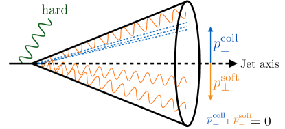
Figure 2: Illustration of the refactorized expression of the jet function 𝒢csubscript𝒢𝑐{\cal G}_{c} in eq. (4) in the limit rRmuch-less-than𝑟𝑅r\ll R. Hard radiation at the jet scale pTRsubscript𝑝𝑇𝑅p_{T}R is allowed outside the observed jet. The collinear radiation (blue) is offset from the jet axis, due to the recoil from the soft radiation (orange) inside the jet, since the jet axis is along the jet momentum.

The resummation of logarithms in r/R𝑟𝑅r/R requires a treatment within SCETII due to the recoil-effect of soft radiation, as pointed out in ref. Kang:2017mda . This resummation is thus similar to that encountered for transverse momentum dependent observables Collins:1984kg ; Becher:2010tm ; Collins:2011zzd ; GarciaEchevarria:2011rb ; Chiu:2012ir ; Kang:2017glf . It is accomplished by refactorizing the jet function 𝒢cjetsuperscriptsubscript𝒢𝑐jet{\mathcal{G}}_{c}^{\rm jet} in eq. (2) in the limit rRmuch-less-than𝑟𝑅r\ll R as

𝒢cjet(z,zr,pTR,r/R,μ)superscriptsubscript𝒢𝑐jet𝑧subscript𝑧𝑟subscript𝑝𝑇𝑅𝑟𝑅𝜇\displaystyle{\mathcal{G}}_{c}^{\mathrm{jet}}(z,z_{r},p_{T}R,r/R,\mu) =NLLdHcd(z,pTR,μ)d2kCd(zr,pTr,k,μ,ν)superscriptsuperscriptNLLabsentsubscript𝑑subscript𝐻𝑐𝑑𝑧subscript𝑝𝑇𝑅𝜇superscriptd2subscript𝑘perpendicular-tosubscript𝐶𝑑subscript𝑧𝑟subscript𝑝𝑇𝑟subscript𝑘perpendicular-to𝜇𝜈\displaystyle\stackrel{{\scriptstyle{\rm NLL}^{\prime}}}{{=}}\sum_{d}H_{cd}(z,p_{T}R,\mu)\,\int\!\mathrm{d}^{2}k_{\perp}\,C_{d}(z_{r},p_{T}r,k_{\perp},\mu,\nu) (4)
×SdG(k,μ,νR)SdNG(rR)[1+𝒪(rR)].absentsuperscriptsubscript𝑆𝑑Gsubscript𝑘perpendicular-to𝜇𝜈𝑅superscriptsubscript𝑆𝑑NG𝑟𝑅delimited-[]1𝒪𝑟𝑅\displaystyle\qquad\times S_{d}^{\rm G}(k_{\perp},\mu,\nu R)\,S_{d}^{\rm NG}\Big{(}\frac{r}{R}\Big{)}\Big{[}1+\mathcal{O}\Big{(}\frac{r}{R}\Big{)}\Big{]}\,.

Here, the hard functions Hcdsubscript𝐻𝑐𝑑H_{cd} describe how the parton c𝑐c coming from the hard-scattering produces a jet of size R𝑅R and of parton flavor d𝑑d, carrying a fraction z𝑧z of the initial parton. The collinear function Cdsubscript𝐶𝑑C_{d} and the soft function SdGsuperscriptsubscript𝑆𝑑GS_{d}^{\rm G} take into account collinear and (global) soft radiation inside the jet. We integrate over the transverse momentum ksubscript𝑘perpendicular-tok_{\perp} generated by the soft radiation, accounting for its recoil on the collinear radiation. By solving the associated renormalization group (RG) equations of the different functions, we achieve the resummation of logarithms in r/R𝑟𝑅r/R. This involves both the standard renormalization group evolution in the invariant mass scale μ𝜇\mu, as well as an evolution in the rapidity scale ν𝜈\nu, as discussed in sec. 2. We calculated the collinear functions Cdsubscript𝐶𝑑C_{d} for the first time at one-loop order, accounting for the dependence on the recoil ksubscript𝑘perpendicular-tok_{\perp}. We also include the contribution of non-global logarithms (NGLs) Dasgupta:2001sh , which are captured by the function SdNGsuperscriptsubscript𝑆𝑑NGS_{d}^{\rm NG} in eq. (4), but only affect the region where r/R𝑟𝑅r/R is very small. The simple (multiplicative) treatment of the NGLs in eq. (4) is the reason this equation is only valid to NLL accuracy. The refactorized cross section in eq. (4) which is given in terms of hard, collinear and soft functions in the limit rRmuch-less-than𝑟𝑅r\ll R is illustrated in fig. 2. In particular, we show the effect of the recoil due to the soft radiation inside the jet.

The perturbative order of the various ingredients needed for the lnR𝑅\ln R and ln(r/R)𝑟𝑅\ln(r/R) resummation is summarized in table 1. We work at NLL accuracy in the ln(r/R)𝑟𝑅\ln(r/R) resummation, as this is commensurate with an NLL resummation of lnR𝑅\ln R. Going beyond this accuracy will be daunting, especially in the treatment of non-global logarithms. We would like to stress that earlier jet shape calculations Seymour:1997kj ; Li:2011hy ; Chien:2014nsa are formally only accurate to leading-logarithmic (LL) order in their treatment of the logarithms of r/R𝑟𝑅r/R. In particular, the contribution from the rapidity evolution, as well as the non-global logarithms, that both first enter at NLL accuracy, are included here for the first time. In addition, earlier calculations did not account for the inclusive jet sample, where the resummation of logarithms of the jet radius R𝑅R changes the ratio of quark and gluon jets, thereby affecting the spectrum already at LL accuracy.

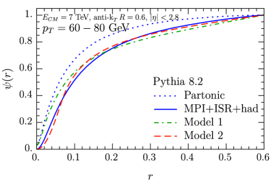
Finally, comparisons between our predictions and LHC data suggested a significant effect of nonperturbative physics (underlying event and hadronization) on the jet shape, particularly for small jet pTsubscript𝑝𝑇p_{T}. This is consistent with the picture that arises from studying these effects in Pythia Sjostrand:2014zea . We will include them in our analysis by using a simple one-parameter model, finding good agreement with the data.

Fixed-order β𝛽\beta γμsubscript𝛾𝜇\gamma_{\mu} γνsubscript𝛾𝜈\gamma_{\nu} NGLs
lnR𝑅\ln R LL tree 111-loop 111-loop - -
NLL 111-loop 222-loop 222-loop - -
NNLL 222-loop 333-loop 333-loop - -
ln(r/R)𝑟𝑅\ln(r/R) LL tree 111-loop 111-loop - -
NLL tree 222-loop 222-loop 111-loop LL
NLL 111-loop 222-loop 222-loop 111-loop LL
NNLL 111-loop 333-loop 333-loop 222-loop NLL
Table 1: The perturbative ingredients needed at various orders in the lnR𝑅\ln R and ln(r/R)𝑟𝑅\ln(r/R) resummation. The columns correspond to the loop order of the fixed-order ingredients, the QCD beta function, the μ𝜇\mu and ν𝜈\nu anomalous dimensions, and the non-global logarithms. The non-cusp part of the μ𝜇\mu anomalous dimension is only needed at one-loop order lower than indicated above.

The remainder of this paper is organized as follows: The theoretical framework used to calculate the jet shape is discussed in sec. 2, with certain ingredients relegated to the appendices. We present a detailed derivation of the collinear function, relevant for the resummation of logarithms in r/R𝑟𝑅r/R, in sec. 3. The details that enter our numerical evaluation of the cross section are described in sec. 4, and first (perturbative) results for quark and gluon jets are presented there. Nonperturbative effects are investigated in sec. 5, for which two simple models are explored. In sec. 6 we show our final results, which we compare to available pp𝑝𝑝pp data from the LHC, and we conclude in sec. 7.

2 Framework

In this section we present the theoretical framework that we use to obtain our results. In sec. 2.1 we describe the factorization formulae and how they enable resummation. We then rearrange these formulae in sec. 2.2, to separate them into the inclusive production of jets and the jet shape itself. In sec. 2.3 the one-loop hard function is given, and in sec. 2.4 we discuss the soft function and non-global logarithms. The calculation of the collinear function at one-loop, accounting for the effect of recoil, is one of the main new results and presented separately in sec. 3. The one-loop expressions for the jet function for rRless-than-or-similar-to𝑟𝑅r\lesssim R are given in app. A, and the anomalous dimensions are listed in app. B.

2.1 Factorization and resummation

The cross section describing the measurement of the fraction zrsubscript𝑧𝑟z_{r} of jet energy inside the cone of radius r𝑟r around the jet axis, in an inclusive sample of jets produced in pp𝑝𝑝pp collisions, factorizes as follows

dσdηdpTdzrd𝜎d𝜂dsubscript𝑝𝑇dsubscript𝑧𝑟\displaystyle\frac{\mathrm{d}\sigma}{\mathrm{d}\eta\,\mathrm{d}p_{T}\,\mathrm{d}z_{r}} =a,b,cdxaxafa(xa,μ)dxbxbfb(xb,μ)dzzabc(xa,xb,η,pT/z,μ)absentsubscript𝑎𝑏𝑐dsubscript𝑥𝑎subscript𝑥𝑎subscript𝑓𝑎subscript𝑥𝑎𝜇dsubscript𝑥𝑏subscript𝑥𝑏subscript𝑓𝑏subscript𝑥𝑏𝜇d𝑧𝑧superscriptsubscript𝑎𝑏𝑐subscript𝑥𝑎subscript𝑥𝑏𝜂subscript𝑝𝑇𝑧𝜇\displaystyle=\sum_{a,b,c}\int\!\frac{\mathrm{d}x_{a}}{x_{a}}\,f_{a}(x_{a},\mu)\int\!\frac{\mathrm{d}x_{b}}{x_{b}}\,f_{b}(x_{b},\mu)\int\!\frac{\mathrm{d}z}{z}\,{\cal H}_{ab}^{c}(x_{a},x_{b},\eta,p_{T}/z,\mu)
×𝒢cjet(z,zr,pTR,r/R,μ)[1+𝒪(R2)].absentsuperscriptsubscript𝒢𝑐jet𝑧subscript𝑧𝑟subscript𝑝𝑇𝑅𝑟𝑅𝜇delimited-[]1𝒪superscript𝑅2\displaystyle\quad\times{\mathcal{G}}_{c}^{\rm jet}(z,z_{r},p_{T}R,r/R,\mu)\big{[}1+\mathcal{O}(R^{2})\big{]}\,. (5)

The parton distribution functions fasubscript𝑓𝑎f_{a} and fbsubscript𝑓𝑏f_{b} describe extracting a parton of flavor a𝑎a and b𝑏b out of the proton, and the function abcsuperscriptsubscript𝑎𝑏𝑐{\cal H}_{ab}^{c} Jager:2002xm encodes their hard scattering in which the parton with flavor c𝑐c, rapidity η𝜂\eta and transverse momentum pT/zsubscript𝑝𝑇𝑧p_{T}/z is produced. The subsequent formation of the jet with transverse momentum z×pT/z=pT𝑧subscript𝑝𝑇𝑧subscript𝑝𝑇z\times p_{T}/z=p_{T} moving in the same direction, as well as the jet shape measurement, is encoded in the jet function 𝒢cjet.superscriptsubscript𝒢𝑐jet{\mathcal{G}}_{c}^{\rm jet}.111In ref. Kang:2017mda this was called the central subjet function and a hat was included on top of 𝒢𝒢{\mathcal{G}}, to distinguish it from other jet functions in that paper. This collinear factorization requires that R1much-less-than𝑅1R\ll 1 to keep the 𝒪(R2)𝒪superscript𝑅2\mathcal{O}(R^{2}) power corrections small. In several examples it has been observed that these power corrections are still small for values of R𝑅R up to 0.7 Mukherjee:2012uz . Note that this factorization formula is identical to that for the inclusive fragmentation of hadrons, with the fragmentation function replaced by our jet function.

The jet function 𝒢cjetsuperscriptsubscript𝒢𝑐jet{\mathcal{G}}_{c}^{\rm jet} describes the formation of the jet as well as the jet shape measurement through zrsubscript𝑧𝑟z_{r}, and has the following matrix-element definition in SCET,

𝒢qjet(z,zr,pTR,r/R,μ)superscriptsubscript𝒢𝑞jet𝑧subscript𝑧𝑟subscript𝑝𝑇𝑅𝑟𝑅𝜇\displaystyle{\mathcal{G}}_{q}^{\mathrm{jet}}(z,z_{r},p_{T}R,r/R,\mu) =16π3X12NcTr[n¯/20|δ(2zn¯𝒫pT)δ2(𝒫)χn(0)|XX|χ¯n(0)|0]\displaystyle=16\pi^{3}\,\sum_{X}\frac{1}{2N_{c}}\,{\rm Tr}\Big{[}\frac{\bar{n}\!\!\!/}{2}\langle 0|\delta\Big{(}2-\frac{z\,\bar{n}\cdot{\mathcal{P}}}{p_{T}}\Big{)}\delta^{2}({\mathcal{P}}_{\perp})\chi_{n}(0)|X\rangle\langle X|\bar{\chi}_{n}(0)|0\rangle\Big{]}
×JRXδ(pTpT(JR))δ(zrpT(jr)pT),\displaystyle\quad\times\sum_{J_{R}\in X}\delta\big{(}p_{T}-p_{T}(J_{R})\big{)}\delta\Big{(}z_{r}-\frac{p_{T}(j_{r})}{p_{T}}\Big{)}\,, (6)

for quark jets, and analogously for gluon jets. Here we exploit that the measurement is invariant under boosts along the beam axis, to set the jet rapidity η𝜂\eta equal to zero.222This avoids spurious factors of coshη𝜂\cosh\eta in intermediate expressions. They arise due to the difference between the energy and transverse momentum of the jet, and are compensated for by the angular size of the jet, which also depends on η𝜂\eta because the jet is defined in (η,ϕ)𝜂italic-ϕ(\eta,\phi) coordinates. We will repeatedly make use of the following decomposition of a vector pμsuperscript𝑝𝜇p^{\mu} in light-cone coordinates

pμ=n¯pnμ2+npn¯μ2+pμ,superscript𝑝𝜇¯𝑛𝑝superscript𝑛𝜇2𝑛𝑝superscript¯𝑛𝜇2superscriptsubscript𝑝perpendicular-to𝜇\displaystyle p^{\mu}=\bar{n}\!\cdot\!p\,\frac{n^{\mu}}{2}+n\!\cdot\!p\,\frac{\bar{n}^{\mu}}{2}+p_{\perp}^{\mu}\,, (7)

where nμ=(1,0,0,1)superscript𝑛𝜇1001n^{\mu}=(1,0,0,1) and n¯μ=(1,0,0,1)superscript¯𝑛𝜇1001\bar{n}^{\mu}=(1,0,0,-1) are light-like vectors, and pμsuperscriptsubscript𝑝perpendicular-to𝜇p_{\perp}^{\mu} denotes the transverse components. The collinear field χ¯nsubscript¯𝜒𝑛\bar{\chi}_{n} in eq. (2.1) describes the quark that initiates the jet, averaged over its spin and color configurations, leading to the factor 1/(2Nc)12subscript𝑁𝑐1/(2N_{c}). It contains a Wilson line to ensure (collinear) gauge invariance. The δ(2zn¯𝒫/pT)𝛿2𝑧¯𝑛𝒫subscript𝑝𝑇\delta(2-z\,\bar{n}\cdot{\mathcal{P}}/p_{T}) fixes the quark field to have transverse momentum pT/zsubscript𝑝𝑇𝑧p_{T}/z with respect to the beam axis, and the δ2(𝒫)superscript𝛿2subscript𝒫perpendicular-to\delta^{2}({\mathcal{P}}_{\perp}) fixes our light-cone coordinates to be along the momentum of the initial parton. The last line describes the sum over all jets JRsubscript𝐽𝑅J_{R} in the final state |Xket𝑋|X\rangle, with transverse momentum pTsubscript𝑝𝑇p_{T}, of which a fraction zrsubscript𝑧𝑟z_{r} is inside the central subjet jrsubscript𝑗𝑟j_{r}. The functions 𝒢qjetsuperscriptsubscript𝒢𝑞jet{\mathcal{G}}_{q}^{\mathrm{jet}} and 𝒢gjetsuperscriptsubscript𝒢𝑔jet{\mathcal{G}}_{g}^{\mathrm{jet}} were calculated at one loop in ref. Kang:2017mda , and their expressions are collected in app. A.

The factorization in eq. (2.1) separates the physics at scales

μfsubscript𝜇𝑓\displaystyle\mu_{f} ΛQCD,similar-toabsentsubscriptΛQCD\displaystyle\sim\Lambda_{\mathrm{QCD}}\,, μsubscript𝜇\displaystyle\mu_{\cal H} pT,similar-toabsentsubscript𝑝𝑇\displaystyle\sim p_{T}\,, μ𝒢subscript𝜇𝒢\displaystyle\mu_{\cal G} pTR.similar-toabsentsubscript𝑝𝑇𝑅\displaystyle\sim p_{T}R\,. (8)

By evolving 𝒢𝒢{\mathcal{G}} from its natural scale μ𝒢subscript𝜇𝒢\mu_{\cal G} to μsubscript𝜇\mu_{\cal H}, the logarithms of μ𝒢/μRsimilar-tosubscript𝜇𝒢subscript𝜇𝑅\mu_{\cal G}/\mu_{\cal H}\sim R are resummed. This involves the DGLAP evolution,

μddμ𝒢ijet(z,zr,pTR,r/R,μ)=jz1dzzαsπPji(z/z)𝒢jjet(z,zr,pTR,r/R,μ),𝜇dd𝜇superscriptsubscript𝒢𝑖jet𝑧subscript𝑧𝑟subscript𝑝𝑇𝑅𝑟𝑅𝜇subscript𝑗superscriptsubscript𝑧1dsuperscript𝑧superscript𝑧subscript𝛼𝑠𝜋subscript𝑃𝑗𝑖𝑧superscript𝑧superscriptsubscript𝒢𝑗jetsuperscript𝑧subscript𝑧𝑟subscript𝑝𝑇𝑅𝑟𝑅𝜇\displaystyle\mu\frac{\mathrm{d}}{\mathrm{d}\mu}\,{\mathcal{G}}_{i}^{\mathrm{jet}}(z,z_{r},p_{T}R,r/R,\mu)=\sum_{j}\int_{z}^{1}\frac{\mathrm{d}z^{\prime}}{z^{\prime}}\,\frac{\alpha_{s}}{\pi}P_{ji}(z/z^{\prime})\,{\mathcal{G}}_{j}^{\mathrm{jet}}(z^{\prime},z_{r},p_{T}R,r/R,\mu)\,, (9)

where the one-loop splitting functions are given by

Pqq(z)subscript𝑃𝑞𝑞𝑧\displaystyle P_{qq}(z) =CF(1+z21z)+,absentsubscript𝐶𝐹subscript1superscript𝑧21𝑧\displaystyle=C_{F}\,\Big{(}\frac{1+z^{2}}{1-z}\Big{)}_{+}\,, Pgq(z)subscript𝑃𝑔𝑞𝑧\displaystyle P_{gq}(z) =CF1+(1z)2z,absentsubscript𝐶𝐹1superscript1𝑧2𝑧\displaystyle=C_{F}\,\frac{1+(1-z)^{2}}{z}\,,
Pgg(z)subscript𝑃𝑔𝑔𝑧\displaystyle P_{gg}(z) =2CA[z(1z)++1zz+z(1z)]+β02δ(1z),absent2subscript𝐶𝐴delimited-[]subscript𝑧1𝑧1𝑧𝑧𝑧1𝑧subscript𝛽02𝛿1𝑧\displaystyle=2C_{A}\bigg{[}\frac{z}{(1-z)}_{+}+\frac{1-z}{z}+z(1-z)\bigg{]}+\frac{\beta_{0}}{2}\,\delta(1-z)\,, Pqg(z)subscript𝑃𝑞𝑔𝑧\displaystyle P_{qg}(z) =TF[z2+(1z)2],absentsubscript𝑇𝐹delimited-[]superscript𝑧2superscript1𝑧2\displaystyle=T_{F}\big{[}z^{2}+(1-z)^{2}\big{]}\,, (10)

and

β0=113CA43TFnf.subscript𝛽0113subscript𝐶𝐴43subscript𝑇𝐹subscript𝑛𝑓\displaystyle\beta_{0}=\frac{11}{3}C_{A}-\frac{4}{3}T_{F}n_{f}\,. (11)
Mode: Scaling (n¯p,np,p)¯𝑛𝑝𝑛𝑝subscript𝑝perpendicular-to(\bar{n}\!\cdot\!p,n\!\cdot\!p,p_{\perp})
hard(-collinear) pT(1,R2,R)subscript𝑝𝑇1superscript𝑅2𝑅p_{T}(1,R^{2},R)
collinear pT(1,r2,r)subscript𝑝𝑇1superscript𝑟2𝑟p_{T}(1,r^{2},r)
(collinear-)soft pT(r/R,rR,r)subscript𝑝𝑇𝑟𝑅𝑟𝑅𝑟p_{T}(r/R,rR,r)
Table 2: The parametric scalings of the momenta of the modes that enter in the factorization of the jet function for rRmuch-less-than𝑟𝑅r\ll R.

For rRmuch-less-than𝑟𝑅r\ll R, the jet function contains large logarithms of r/R𝑟𝑅r/R that also require resummation. This is achieved through a second factorization Kang:2017mda 333This is identical to eq. (4) and repeated for convenience. Note that we adopted a slightly different convention for the arguments of the involved functions in comparison to ref. Kang:2017mda .

𝒢cjet(z,zr,pTR,r/R,μ)superscriptsubscript𝒢𝑐jet𝑧subscript𝑧𝑟subscript𝑝𝑇𝑅𝑟𝑅𝜇\displaystyle{\mathcal{G}}_{c}^{\mathrm{jet}}(z,z_{r},p_{T}R,r/R,\mu) =NLLdHcd(z,pTR,μ)d2kCd(zr,pTr,k,μ,ν)superscriptsuperscriptNLLabsentsubscript𝑑subscript𝐻𝑐𝑑𝑧subscript𝑝𝑇𝑅𝜇superscriptd2subscript𝑘perpendicular-tosubscript𝐶𝑑subscript𝑧𝑟subscript𝑝𝑇𝑟subscript𝑘perpendicular-to𝜇𝜈\displaystyle\stackrel{{\scriptstyle{\rm NLL}^{\prime}}}{{=}}\sum_{d}H_{cd}(z,p_{T}R,\mu)\,\int\!\mathrm{d}^{2}k_{\perp}\,C_{d}(z_{r},p_{T}r,k_{\perp},\mu,\nu) (12)
×SdG(k,μ,νR)SdNG(rR)[1+𝒪(rR)].absentsuperscriptsubscript𝑆𝑑Gsubscript𝑘perpendicular-to𝜇𝜈𝑅superscriptsubscript𝑆𝑑NG𝑟𝑅delimited-[]1𝒪𝑟𝑅\displaystyle\qquad\times S_{d}^{\rm G}(k_{\perp},\mu,\nu R)\,S_{d}^{\rm NG}\Big{(}\frac{r}{R}\Big{)}\Big{[}1+\mathcal{O}\Big{(}\frac{r}{R}\Big{)}\Big{]}\,.

The momentum scalings of the modes in SCET, corresponding to the various ingredients in eq. (12), are listed in table 2. If we boost to a frame where the jet and out-of-jet region are complementary hemispheres, this is the usual power counting for hard, collinear and soft radiation, which is why we use this nomenclature instead of hard-collinear and collinear-soft. The hard function Hcdsubscript𝐻𝑐𝑑H_{cd} describes how the initial parton c𝑐c produces a jet of radius R𝑅R with parton flavor d𝑑d and a fraction z𝑧z of the initial transverse momentum with respect to the beam axis. Within the jet, the parton d𝑑d can only undergo energetic splittings of angles of order r𝑟r, otherwise the collinear radiation would lie outside the cone of radius r𝑟r.444Of course there could be a splitting inside the jet of angular size R that is balanced in such a way that there is also collinear radiation inside the cone of size r𝑟r at the center of the jet, but such configurations give a power suppressed contribution. This is very similar to the power suppression of the contribution from two nearly back-to-back jets in Higgs production at small transverse momentum, discussed in e.g. ref. Chiu:2012ir . The fraction zrsubscript𝑧𝑟z_{r} of this collinear radiation within the cone of size r𝑟r is described by the collinear function Cdsubscript𝐶𝑑C_{d}. The collinear function also accounts for the transverse momentum offset ksubscript𝑘perpendicular-tok_{\perp} of the initial collinear parton with respect to the jet axis, due to recoil against soft radiation. In sec. 3 we will present the first one-loop calculation of the collinear function for k0subscript𝑘perpendicular-to0k_{\perp}\neq 0. The distribution of this recoil is encoded in the soft function, which we separate into a global contribution SdGsuperscriptsubscript𝑆𝑑GS_{d}^{\rm G} and non-global logarithms SdNGsuperscriptsubscript𝑆𝑑NGS_{d}^{\rm NG}. Non-global logarithms Dasgupta:2001sh arise because only soft radiation inside the jet affects the position of the axis, and our simple treatment of them is the reason why eq. (12) only holds to NLL accuracy, see sec. 2.4. The 𝒪(r/R)𝒪𝑟𝑅\mathcal{O}(r/R) power corrections in eq. (12) can be extracted from 𝒢cjetsuperscriptsubscript𝒢𝑐jet{\mathcal{G}}_{c}^{\mathrm{jet}}, and will be included.

Transverse momentum dependent observables generically suffer from rapidity divergences. We will employ the η𝜂\eta-regulator Chiu:2011qc ; Chiu:2012ir , for which ν𝜈\nu denotes the corresponding rapidity renormalization scale. The factorization in eq. (12) separates the jet function into ingredients at the scales

μHsubscript𝜇𝐻\displaystyle\mu_{H} pTR,similar-toabsentsubscript𝑝𝑇𝑅\displaystyle\sim p_{T}R\,, μCsubscript𝜇𝐶\displaystyle\mu_{C} pTr,similar-toabsentsubscript𝑝𝑇𝑟\displaystyle\sim p_{T}\,r\,, μSGsubscript𝜇superscript𝑆G\displaystyle\mu_{S^{\rm G}} pTr,similar-toabsentsubscript𝑝𝑇𝑟\displaystyle\sim p_{T}\,r\,,
νCsubscript𝜈𝐶\displaystyle\nu_{C} pT,similar-toabsentsubscript𝑝𝑇\displaystyle\sim p_{T}\,, νSGsubscript𝜈superscript𝑆G\displaystyle\nu_{S^{\rm G}} pTrR.similar-toabsentsubscript𝑝𝑇𝑟𝑅\displaystyle\sim p_{T}\,\frac{r}{R}\,. (13)

By evaluating the ingredients at their natural scales and using the RG evolution to evolve them to a common scale, the global logarithms of μC/μHμSG/μHνSG/νCr/Rsimilar-tosubscript𝜇𝐶subscript𝜇𝐻subscript𝜇superscript𝑆Gsubscript𝜇𝐻similar-tosubscript𝜈superscript𝑆Gsubscript𝜈𝐶similar-to𝑟𝑅\mu_{C}/\mu_{H}\sim\mu_{S^{\rm G}}/\mu_{H}\sim\nu_{S^{\rm G}}/\nu_{C}\sim r/R are resummed. The RG equations are555The expressions in ref. Kang:2017mda contain a typo, as the convolution in ksubscript𝑘perpendicular-tok_{\perp} for the ν𝜈\nu-RG equations was omitted.

μddμHcd(z,pTR,μ)𝜇dd𝜇subscript𝐻𝑐𝑑𝑧subscript𝑝𝑇𝑅𝜇\displaystyle\mu\frac{\mathrm{d}}{\mathrm{d}\mu}\,H_{cd}(z,p_{T}R,\mu) =ez1dzzγceH(zz,pTR,μ)Hed(z,pTR,μ).absentsubscript𝑒superscriptsubscript𝑧1dsuperscript𝑧superscript𝑧subscriptsuperscript𝛾𝐻𝑐𝑒𝑧superscript𝑧subscript𝑝𝑇𝑅𝜇subscript𝐻𝑒𝑑superscript𝑧subscript𝑝𝑇𝑅𝜇\displaystyle=\sum_{e}\int_{z}^{1}\frac{\mathrm{d}z^{\prime}}{z^{\prime}}\,\gamma^{H}_{ce}\Big{(}\frac{z}{z^{\prime}},p_{T}R,\mu\Big{)}\,H_{ed}(z^{\prime},p_{T}R,\mu)\,.
μddμCd(zr,pTr,k,μ,ν)𝜇dd𝜇subscript𝐶𝑑subscript𝑧𝑟subscript𝑝𝑇𝑟subscript𝑘perpendicular-to𝜇𝜈\displaystyle\mu\frac{\mathrm{d}}{\mathrm{d}\mu}\,C_{d}(z_{r},p_{T}r,k_{\perp},\mu,\nu) =γdC(μ,ν/pT)Cd(zr,pTr,k,μ,ν).absentsubscriptsuperscript𝛾𝐶𝑑𝜇𝜈subscript𝑝𝑇subscript𝐶𝑑subscript𝑧𝑟subscript𝑝𝑇𝑟subscript𝑘perpendicular-to𝜇𝜈\displaystyle=\gamma^{C}_{d}(\mu,\nu/p_{T})\,C_{d}(z_{r},p_{T}r,k_{\perp},\mu,\nu)\,.
μddμSdG(k,μ,νR)𝜇dd𝜇superscriptsubscript𝑆𝑑Gsubscript𝑘perpendicular-to𝜇𝜈𝑅\displaystyle\mu\frac{\mathrm{d}}{\mathrm{d}\mu}\,S_{d}^{\rm G}(k_{\perp},\mu,\nu R) =γdS(μ,νR)SdG(k,μ,νR),absentsubscriptsuperscript𝛾𝑆𝑑𝜇𝜈𝑅superscriptsubscript𝑆𝑑Gsubscript𝑘perpendicular-to𝜇𝜈𝑅\displaystyle=\gamma^{S}_{d}(\mu,\nu R)\,S_{d}^{\rm G}(k_{\perp},\mu,\nu R)\,,
νddνCd(zr,pTr,k,μ,ν)𝜈dd𝜈subscript𝐶𝑑subscript𝑧𝑟subscript𝑝𝑇𝑟subscript𝑘perpendicular-to𝜇𝜈\displaystyle\nu\frac{\mathrm{d}}{\mathrm{d}\nu}\,C_{d}(z_{r},p_{T}r,k_{\perp},\mu,\nu) =d2k(2π)2γdν(kk,μ)Cd(zr,pTr,k,μ,ν).absentsuperscriptd2superscriptsubscript𝑘perpendicular-tosuperscript2𝜋2subscriptsuperscript𝛾𝜈𝑑subscript𝑘perpendicular-tosuperscriptsubscript𝑘perpendicular-to𝜇subscript𝐶𝑑subscript𝑧𝑟subscript𝑝𝑇𝑟superscriptsubscript𝑘perpendicular-to𝜇𝜈\displaystyle=-\int\!\frac{\mathrm{d}^{2}k_{\perp}^{\prime}}{(2\pi)^{2}}\,\gamma^{\nu}_{d}(k_{\perp}-k_{\perp}^{\prime},\mu)\,C_{d}(z_{r},p_{T}r,k_{\perp}^{\prime},\mu,\nu)\,.
νddνSdG(k,μ,νR)𝜈dd𝜈superscriptsubscript𝑆𝑑Gsubscript𝑘perpendicular-to𝜇𝜈𝑅\displaystyle\nu\frac{\mathrm{d}}{\mathrm{d}\nu}\,S_{d}^{\rm G}(k_{\perp},\mu,\nu R) =d2k(2π)2γdν(kk,μ)SdG(k,μ,νR).absentsuperscriptd2superscriptsubscript𝑘perpendicular-tosuperscript2𝜋2subscriptsuperscript𝛾𝜈𝑑subscript𝑘perpendicular-tosuperscriptsubscript𝑘perpendicular-to𝜇superscriptsubscript𝑆𝑑Gsuperscriptsubscript𝑘perpendicular-to𝜇𝜈𝑅\displaystyle=\int\!\frac{\mathrm{d}^{2}k_{\perp}^{\prime}}{(2\pi)^{2}}\,\gamma^{\nu}_{d}(k_{\perp}-k_{\perp}^{\prime},\mu)\,S_{d}^{\rm G}(k_{\perp}^{\prime},\mu,\nu R)\,. (14)

The anomalous dimensions are collected in app. B. As is clear from eq. (12), the anomalous dimensions of the hard, collinear and soft function should combine to give the anomalous dimension of the jet function, which we checked. The μ𝜇\mu-evolution sums double logarithms, and the ν𝜈\nu-evolution, which was missed prior to our work in ref. Kang:2017mda , sums single logarithms. We also include the leading non-global logarithms to obtain the desired NLL accuracy, which will be discussed in sec. 2.4.

2.2 Separating the jet production and jet shape

We now rearrange our calculation in a way that simplifies the numerical implementation, effectively separating the jet production and the jet shape.666A similar rearrangement was carried out for hadron fragmentation inside a jet in ref. Kaufmann:2015hma . We start by writing 𝒢cjetsuperscriptsubscript𝒢𝑐jet{\mathcal{G}}_{c}^{\rm jet} as

𝒢cjet(z,zr,pTR,r/R,μ)superscriptsubscript𝒢𝑐jet𝑧subscript𝑧𝑟subscript𝑝𝑇𝑅𝑟𝑅𝜇\displaystyle{\mathcal{G}}_{c}^{\rm jet}(z,z_{r},p_{T}R,r/R,\mu) =dJcd(z,pTR,μ)dz[𝒢djet(z,zr,pTR,r/R,μ)\displaystyle=\sum_{d}J_{cd}(z,p_{T}R,\mu)\int\!\mathrm{d}z^{\prime}\,\Bigl{[}{\mathcal{G}}_{d}^{\rm jet}(z^{\prime},z_{r},p_{T}R,r/R,\mu)
Jd(1)(z,pTR,μ)δ(1zr)]+𝒪(αs2).\displaystyle\quad-J_{d}^{(1)}(z^{\prime},p_{T}R,\mu)\,\delta(1-z_{r})\Bigr{]}+\mathcal{O}(\alpha_{s}^{2})\,. (15)

Here Jdsubscript𝐽𝑑J_{d} is the semi-inclusive jet function Kang:2016mcy ; Dai:2016hzf that enters in inclusive jet production. Jcdsubscript𝐽𝑐𝑑J_{cd} is directly related, except that it not only keeps track of the flavor c𝑐c of the initiating parton but also the flavor d𝑑d of the jet, so

dJcd(z,pTR,μ)=Jc(z,pTR,μ).subscript𝑑subscript𝐽𝑐𝑑𝑧subscript𝑝𝑇𝑅𝜇subscript𝐽𝑐𝑧subscript𝑝𝑇𝑅𝜇\displaystyle\sum_{d}J_{cd}(z,p_{T}R,\mu)=J_{c}(z,p_{T}R,\mu)\,. (16)

Its one-loop expressions are given in eq. (25). Note that eq. (2.2) is not a factorization of physics at different scales, as the natural scale of 𝒢jetsuperscript𝒢jet\mathcal{G}^{\rm jet} and J𝐽J is both pTRsubscript𝑝𝑇𝑅p_{T}R. However, this is why it is justified to work to finite order in αssubscript𝛼𝑠\alpha_{s}. We exploited that at one-loop order the nontrivial z𝑧z-dependence cancels between 𝒢djetsubscriptsuperscript𝒢jet𝑑{\mathcal{G}}^{\rm jet}_{d} and Jdsubscript𝐽𝑑J_{d}, i.e. their difference is proportional to δ(1z)𝛿1𝑧\delta(1-z), since the splitting where one parton is outside the jet is treated the same in both calculations. This delta function is removed by the integral over z𝑧z. Combining Jcdsubscript𝐽𝑐𝑑J_{cd} with the rest of eq. (2.1), we identify this as the cross section for the inclusive production of jets of flavor d𝑑d,

dσddηdpTdsubscript𝜎𝑑d𝜂dsubscript𝑝𝑇\displaystyle\frac{\mathrm{d}\sigma_{d}}{\mathrm{d}\eta\,\mathrm{d}p_{T}} =a,b,cdxaxafa(xa,μ)dxbxbfb(xb,μ)dzzabc(xa,xb,η,pT/z,μ)absentsubscript𝑎𝑏𝑐dsubscript𝑥𝑎subscript𝑥𝑎subscript𝑓𝑎subscript𝑥𝑎𝜇dsubscript𝑥𝑏subscript𝑥𝑏subscript𝑓𝑏subscript𝑥𝑏𝜇d𝑧𝑧superscriptsubscript𝑎𝑏𝑐subscript𝑥𝑎subscript𝑥𝑏𝜂subscript𝑝𝑇𝑧𝜇\displaystyle=\sum_{a,b,c}\int\!\frac{\mathrm{d}x_{a}}{x_{a}}\,f_{a}(x_{a},\mu)\int\!\frac{\mathrm{d}x_{b}}{x_{b}}\,f_{b}(x_{b},\mu)\int\!\frac{\mathrm{d}z}{z}\,{\cal H}_{ab}^{c}(x_{a},x_{b},\eta,p_{T}/z,\mu)
×Jcd(z,pTR,μ)[1+𝒪(R2)].absentsubscript𝐽𝑐𝑑𝑧subscript𝑝𝑇𝑅𝜇delimited-[]1𝒪superscript𝑅2\displaystyle\quad\times J_{cd}(z,p_{T}R,\mu)\big{[}1+\mathcal{O}(R^{2})\big{]}\,. (17)

By summing over d𝑑d and using eq. (16), this reproduces the inclusive jet cross section in refs. Kang:2016mcy ; Dai:2016hzf . Eq. (3) then implies that this remainder corresponds to the jet shape ψc(r)subscript𝜓𝑐𝑟\psi_{c}(r) for a jet of flavor c𝑐c, after taking the second Mellin moment of zrsubscript𝑧𝑟z_{r},

ψd(r)=dz[dzrzr𝒢djet(z,zr,pTR,r/R,μ)Jd(1)(z,pTR,μ)]+𝒪(αs2).subscript𝜓𝑑𝑟differential-d𝑧delimited-[]differential-dsubscript𝑧𝑟subscript𝑧𝑟superscriptsubscript𝒢𝑑jet𝑧subscript𝑧𝑟subscript𝑝𝑇𝑅𝑟𝑅𝜇superscriptsubscript𝐽𝑑1𝑧subscript𝑝𝑇𝑅𝜇𝒪superscriptsubscript𝛼𝑠2\displaystyle\psi_{d}(r)=\int\!\mathrm{d}z\,\biggl{[}\int\!\mathrm{d}z_{r}\,z_{r}\,{\mathcal{G}}_{d}^{\rm jet}(z,z_{r},p_{T}R,r/R,\mu)-J_{d}^{(1)}(z,p_{T}R,\mu)\biggr{]}+\mathcal{O}(\alpha_{s}^{2})\,. (18)

Using the expressions in app. A, the jet shape for rRless-than-or-similar-to𝑟𝑅r\lesssim R is given by

ψq,rR(r)subscript𝜓less-than-or-similar-to𝑞𝑟𝑅𝑟\displaystyle\psi_{q,r\lesssim R}(r) =1+αsCF2π[12Lr/R2+32Lr/R92+6rR3r22R2],absent1subscript𝛼𝑠subscript𝐶𝐹2𝜋delimited-[]12superscriptsubscript𝐿𝑟𝑅232subscript𝐿𝑟𝑅926𝑟𝑅3superscript𝑟22superscript𝑅2\displaystyle=1+\frac{\alpha_{s}C_{F}}{2\pi}\bigg{[}-\frac{1}{2}L_{r/R}^{2}+\frac{3}{2}L_{r/R}-\frac{9}{2}+\frac{6r}{R}-\frac{3r^{2}}{2R^{2}}\bigg{]}\,,
ψg,rR(r)subscript𝜓less-than-or-similar-to𝑔𝑟𝑅𝑟\displaystyle\psi_{g,r\lesssim R}(r) =1+αs2π[CA2Lr/R2+β02Lr/R+CA(20336+8rR3r2R2+8r39R3r44R4)\displaystyle=1+\frac{\alpha_{s}}{2\pi}\bigg{[}-\frac{C_{A}}{2}L_{r/R}^{2}+\frac{\beta_{0}}{2}L_{r/R}+C_{A}\Big{(}-\frac{203}{36}+\frac{8r}{R}-\frac{3r^{2}}{R^{2}}+\frac{8r^{3}}{9R^{3}}-\frac{r^{4}}{4R^{4}}\Big{)}
+TFnf(41184rR+3r2R216r39R3+r42R4)],\displaystyle\quad+T_{F}n_{f}\Big{(}\frac{41}{18}-\frac{4r}{R}+\frac{3r^{2}}{R^{2}}-\frac{16r^{3}}{9R^{3}}+\frac{r^{4}}{2R^{4}}\Big{)}\bigg{]}\,, (19)

which is properly normalized, ψd,rR(R)=1subscript𝜓less-than-or-similar-to𝑑𝑟𝑅𝑅1\psi_{d,r\lesssim R}(R)=1.

For rRmuch-less-than𝑟𝑅r\ll R, the factorization of 𝒢𝒢{\mathcal{G}} in eq. (12) leads to the following expression for the jet shape

ψd,rR(r)subscript𝜓much-less-than𝑑𝑟𝑅𝑟\displaystyle\psi_{d,r\ll R}(r) =NLLH~d(pTR,μ)d2kdzrzrCd(zr,pTr,k,μ,ν)superscriptsuperscriptNLLabsentsubscript~𝐻𝑑subscript𝑝𝑇𝑅𝜇superscriptd2subscript𝑘perpendicular-todifferential-dsubscript𝑧𝑟subscript𝑧𝑟subscript𝐶𝑑subscript𝑧𝑟subscript𝑝𝑇𝑟subscript𝑘perpendicular-to𝜇𝜈\displaystyle\stackrel{{\scriptstyle{\rm NLL}^{\prime}}}{{=}}\tilde{H}_{d}(p_{T}R,\mu)\,\int\!\mathrm{d}^{2}k_{\perp}\,\int\!\mathrm{d}z_{r}\,z_{r}\,C_{d}(z_{r},p_{T}r,k_{\perp},\mu,\nu) (20)
×SdG(k,μ,νR)SdNG(rR)[1+𝒪(rR)],absentsuperscriptsubscript𝑆𝑑Gsubscript𝑘perpendicular-to𝜇𝜈𝑅superscriptsubscript𝑆𝑑NG𝑟𝑅delimited-[]1𝒪𝑟𝑅\displaystyle\qquad\times S_{d}^{\rm G}(k_{\perp},\mu,\nu R)\,S_{d}^{\rm NG}\Big{(}\frac{r}{R}\Big{)}\Big{[}1+\mathcal{O}\Big{(}\frac{r}{R}\Big{)}\Big{]}\,,

where

H~d(pTR,μ)=dze[Hde(z,pTR,μ)Jde(1)(z,pTR,μ)].subscript~𝐻𝑑subscript𝑝𝑇𝑅𝜇differential-d𝑧subscript𝑒delimited-[]subscript𝐻𝑑𝑒𝑧subscript𝑝𝑇𝑅𝜇superscriptsubscript𝐽𝑑𝑒1𝑧subscript𝑝𝑇𝑅𝜇\displaystyle\tilde{H}_{d}(p_{T}R,\mu)=\int\!\mathrm{d}z\sum_{e}\Bigl{[}H_{de}(z,p_{T}R,\mu)-J_{de}^{(1)}(z,p_{T}R,\mu)\Bigr{]}\,. (21)

The contribution of Hde(1)superscriptsubscript𝐻𝑑𝑒1H_{de}^{(1)} is removed by subtracting Jde(1)superscriptsubscript𝐽𝑑𝑒1J_{de}^{(1)}, but there is a constant remainder δdeδ(1z)proportional-toabsentsubscript𝛿𝑑𝑒𝛿1𝑧\propto\delta_{de}\delta(1-z) since Jde(1)superscriptsubscript𝐽𝑑𝑒1J_{de}^{(1)} also receives a contribution when both partons are inside the jet. This constant is contained in H~dsubscript~𝐻𝑑\tilde{H}_{d}, where it is multiplied by the Sudakov factor from the evolution kernels, ensuring that it’s contribution vanishes for r0𝑟0r\to 0 (as required). In our implementation of eq. (20), we 1) include the evolution kernels from evolving the ingredients between their natural scales, 2) expand the fixed-order ingredients, i.e. dropping cross terms such as C(1)S(1)superscript𝐶1superscript𝑆1C^{(1)}S^{(1)}, and 3) include the corrections contained in 𝒪(r/R)𝒪𝑟𝑅\mathcal{O}(r/R), which can be read of from eq. (2.2).

2.3 Hard function

The hard function Hcdsubscript𝐻𝑐𝑑H_{cd} in eq. (12) is up to one-loop order given by Kang:2017mda ; Kang:2017glf

Hqq(z,pTR,μ)subscript𝐻𝑞𝑞𝑧subscript𝑝𝑇𝑅𝜇\displaystyle H_{qq}(z,p_{T}R,\mu) =δ(1z)+αs2π[CFδ(1z)(LR2232LR+π212)\displaystyle=\delta(1-z)+\frac{\alpha_{s}}{2\pi}\bigg{[}C_{F}\delta(1-z)\Big{(}-\frac{L_{R}^{2}}{2}-\frac{3}{2}L_{R}+\frac{\pi^{2}}{12}\Big{)}
+LRPqq(z)2CF(1+z2)(ln(1z)1z)+CF(1z)],\displaystyle\quad+L_{R}P_{qq}(z)-2C_{F}(1+z^{2})\Big{(}\frac{\ln(1-z)}{1-z}\Big{)}_{+}-C_{F}(1-z)\bigg{]},
Hqg(z,pTR,μ)subscript𝐻𝑞𝑔𝑧subscript𝑝𝑇𝑅𝜇\displaystyle H_{qg}(z,p_{T}R,\mu) =αs2π[(LR2ln(1z))Pgq(z)CFz],absentsubscript𝛼𝑠2𝜋delimited-[]subscript𝐿𝑅21𝑧subscript𝑃𝑔𝑞𝑧subscript𝐶𝐹𝑧\displaystyle=\frac{\alpha_{s}}{2\pi}\bigg{[}\Big{(}L_{R}-2\ln(1-z)\Big{)}P_{gq}(z)-C_{F}z\bigg{]},
Hgq(z,pTR,μ)subscript𝐻𝑔𝑞𝑧subscript𝑝𝑇𝑅𝜇\displaystyle H_{gq}(z,p_{T}R,\mu) =αs2π[(LR2ln(1z))Pqg(z)TF2z(1z)],absentsubscript𝛼𝑠2𝜋delimited-[]subscript𝐿𝑅21𝑧subscript𝑃𝑞𝑔𝑧subscript𝑇𝐹2𝑧1𝑧\displaystyle=\frac{\alpha_{s}}{2\pi}\bigg{[}\Big{(}L_{R}-2\ln(1-z)\Big{)}P_{qg}(z)-T_{F}2z(1-z)\bigg{]},
Hgg(z,pTR,μ)subscript𝐻𝑔𝑔𝑧subscript𝑝𝑇𝑅𝜇\displaystyle H_{gg}(z,p_{T}R,\mu) =δ(1z)+αs2π[δ(1z)(CALR22β02LR+CAπ212)\displaystyle=\delta(1-z)+\frac{\alpha_{s}}{2\pi}\bigg{[}\delta(1-z)\Big{(}-C_{A}\frac{L_{R}^{2}}{2}-\frac{\beta_{0}}{2}L_{R}+C_{A}\frac{\pi^{2}}{12}\Big{)}
+LRPgg(z)4CA(1z+z2)2z(ln(1z)1z)+].\displaystyle\quad+L_{R}P_{gg}(z)-\frac{4C_{A}(1-z+z^{2})^{2}}{z}\left(\frac{\ln(1-z)}{1-z}\right)_{+}\bigg{]}. (22)

where the splitting functions are given in eq. (2.1), β0subscript𝛽0\beta_{0} is given in eq. (11) and LRsubscript𝐿𝑅L_{R} is

LR=ln(μ2pT2R2).subscript𝐿𝑅superscript𝜇2superscriptsubscript𝑝𝑇2superscript𝑅2\displaystyle L_{R}=\ln\Big{(}\frac{\mu^{2}}{p_{T}^{2}R^{2}}\Big{)}\,. (23)

The hard function is formally a matching coefficient. At one-loop order it is simply the contribution to 𝒢csubscript𝒢𝑐{\mathcal{G}}_{c} from the region of phase space where the two partons produced by a splitting of c𝑐c are not clustered together. The second index d𝑑d denotes the parton inside the jet.

The hard function H~dsubscript~𝐻𝑑\tilde{H}_{d} in eq. (21) is given by

H~q(pTR,μ)subscript~𝐻𝑞subscript𝑝𝑇𝑅𝜇\displaystyle\tilde{H}_{q}(p_{T}R,\mu) =1+αsCF2π(12LR232LR132+3π24)+𝒪(αs2),absent1subscript𝛼𝑠subscript𝐶𝐹2𝜋12superscriptsubscript𝐿𝑅232subscript𝐿𝑅1323superscript𝜋24𝒪superscriptsubscript𝛼𝑠2\displaystyle=1+\frac{\alpha_{s}C_{F}}{2\pi}\biggl{(}-\frac{1}{2}L_{R}^{2}-\frac{3}{2}L_{R}-\frac{13}{2}+\frac{3\pi^{2}}{4}\biggr{)}+\mathcal{O}(\alpha_{s}^{2})\,,
H~g(pTR,μ)subscript~𝐻𝑔subscript𝑝𝑇𝑅𝜇\displaystyle\tilde{H}_{g}(p_{T}R,\mu) =1+αs2π[CA(12LR2512+3π24)+β0(12LR2312)]+𝒪(αs2).absent1subscript𝛼𝑠2𝜋delimited-[]subscript𝐶𝐴12superscriptsubscript𝐿𝑅25123superscript𝜋24subscript𝛽012subscript𝐿𝑅2312𝒪superscriptsubscript𝛼𝑠2\displaystyle=1+\frac{\alpha_{s}}{2\pi}\biggl{[}C_{A}\bigg{(}-\frac{1}{2}L_{R}^{2}-\frac{5}{12}+\frac{3\pi^{2}}{4}\bigg{)}+\beta_{0}\bigg{(}-\frac{1}{2}L_{R}-\frac{23}{12}\bigg{)}\biggr{]}+\mathcal{O}(\alpha_{s}^{2})\,. (24)

For completeness we mention that at one-loop order the semi-inclusive jet function with identified jet flavor Jcdsubscript𝐽𝑐𝑑J_{cd} is

Jcd(1)(z,pTR,μ)=Hcd(1)(z,pTR,μ)δcdδ(1z)H~c(1)(pTR,μ),superscriptsubscript𝐽𝑐𝑑1𝑧subscript𝑝𝑇𝑅𝜇superscriptsubscript𝐻𝑐𝑑1𝑧subscript𝑝𝑇𝑅𝜇subscript𝛿𝑐𝑑𝛿1𝑧superscriptsubscript~𝐻𝑐1subscript𝑝𝑇𝑅𝜇\displaystyle J_{cd}^{(1)}(z,p_{T}R,\mu)=H_{cd}^{(1)}(z,p_{T}R,\mu)-\delta_{cd}\delta(1-z)\tilde{H}_{c}^{(1)}(p_{T}R,\mu)\,, (25)

in terms of the above equations.

2.4 Soft function and non-global logarithms

Up to NLL order, the global soft function for quark jets can be calculated from

SqG(k,μ,νR)=NLL1NcXs0|T¯[Yn¯Yn]|XX|T[YnYn¯]|0δ2(kijetki,),superscriptsuperscriptNLLsuperscriptsubscript𝑆𝑞Gsubscript𝑘perpendicular-to𝜇𝜈𝑅1subscript𝑁𝑐subscriptsubscript𝑋𝑠quantum-operator-product0¯Tdelimited-[]superscriptsubscript𝑌¯𝑛subscript𝑌𝑛𝑋quantum-operator-product𝑋Tdelimited-[]superscriptsubscript𝑌𝑛subscript𝑌¯𝑛0superscript𝛿2subscript𝑘perpendicular-tosubscript𝑖jetsubscript𝑘𝑖perpendicular-to\displaystyle S_{q}^{\rm G}(k_{\perp},\mu,\nu R)\stackrel{{\scriptstyle{\rm NLL}^{\prime}}}{{=}}\frac{1}{N_{c}}\sum_{X_{s}}\langle 0|{\rm\bar{T}}[Y_{\bar{n}}^{\dagger}Y_{n}]\,|X\rangle\langle X|{\rm T}[Y_{n}^{\dagger}Y_{\bar{n}}]|0\rangle\delta^{2}\Big{(}k_{\perp}-\sum_{i\in{\rm jet}}k_{i,\perp}\Big{)}\,, (26)

where the delta function sums the transverse momentum ki,subscript𝑘𝑖perpendicular-tok_{i,\perp} with respect to the jet axis of soft radiation in X𝑋X that is inside the jet. Soft radiation does not resolve individual collinear splittings, and so soft radiation emitted by the collinear particles in the jet can be encoded by the eikonal Wilson line Ynsuperscriptsubscript𝑌𝑛Y_{n}^{\dagger}. At NLL, the one-loop calculation of the soft function comes with the tree-level hard function, so there is a single parton moving in the n¯¯𝑛\bar{n} direction, resulting in Yn¯subscript𝑌¯𝑛Y_{\bar{n}}. At higher orders, real emissions in the hard function (outside the jet) will result in additional Wilson lines Larkoski:2015zka ; Becher:2015hka , see also ref. Caron-Huot:2015bja . This complicates the non-global logarithms, but is fortunately beyond the accuracy at which we are working.

A one-loop calculation yields Kang:2017mda

SqG(k,μ,νR)=δ2(k)+αsCF2π2[1μ2(ln(k2/μ2)k2/μ2)++1μ21(k2/μ2)+lnν2R24μ2π212δ(k 2)].superscriptsubscript𝑆𝑞Gsubscript𝑘perpendicular-to𝜇𝜈𝑅superscript𝛿2subscript𝑘perpendicular-tosubscript𝛼𝑠subscript𝐶𝐹2superscript𝜋2delimited-[]1superscript𝜇2subscriptsuperscriptsubscript𝑘perpendicular-to2superscript𝜇2superscriptsubscript𝑘perpendicular-to2superscript𝜇21superscript𝜇2subscript1superscriptsubscript𝑘perpendicular-to2superscript𝜇2superscript𝜈2superscript𝑅24superscript𝜇2superscript𝜋212𝛿superscriptsubscript𝑘perpendicular-to2\displaystyle S_{q}^{\rm G}(k_{\perp},\mu,\nu R)=\delta^{2}(k_{\perp})\!+\!\frac{\alpha_{s}C_{F}}{2\pi^{2}}\bigg{[}-\frac{1}{\mu^{2}}\,\Big{(}\frac{\ln(k_{\perp}^{2}/\mu^{2})}{k_{\perp}^{2}/\mu^{2}}\Big{)}_{+}\!\!+\!\frac{1}{\mu^{2}}\,\frac{1}{(k_{\perp}^{2}/\mu^{2})}_{+}\!\!\ln\frac{\nu^{2}R^{2}}{4\mu^{2}}\!-\!\frac{\pi^{2}}{12}\delta(\vec{k}_{\perp}^{\,2})\bigg{]}\,. (27)

For SgGsuperscriptsubscript𝑆𝑔GS_{g}^{\rm G} the Wilson lines are in the adjoint representation, instead of the fundamental representation, and the overall normalization in the definition is modified from 1/Nc1subscript𝑁𝑐1/N_{c} to 1/(Nc21)1superscriptsubscript𝑁𝑐211/(N_{c}^{2}-1). The one-loop result for SgGsuperscriptsubscript𝑆𝑔GS_{g}^{\rm G} is simply given by replacing CFCAsubscript𝐶𝐹subscript𝐶𝐴C_{F}\to C_{A} in eq. (27).

The non-global logarithms arise from soft emission patterns that simultaneously probe the jet and out-of-jet region Dasgupta:2001sh . Since we consider R1much-less-than𝑅1R\ll 1, the NGLs are the same as in the hemisphere case Banfi:2010pa . Indeed, a direct calculation of the leading contribution at order αs2superscriptsubscript𝛼𝑠2\alpha_{s}^{2} gives rise to

αs2CACi24π1(pTR)2(ln(k2/(pTR)2)k2/(pTR)2)+,superscriptsubscript𝛼𝑠2subscript𝐶𝐴subscript𝐶𝑖24𝜋1superscriptsubscript𝑝𝑇𝑅2subscriptsuperscriptsubscript𝑘perpendicular-to2superscriptsubscript𝑝𝑇𝑅2superscriptsubscript𝑘perpendicular-to2superscriptsubscript𝑝𝑇𝑅2\displaystyle-\frac{\alpha_{s}^{2}C_{A}C_{i}}{24\pi}\,\frac{1}{(p_{T}R)^{2}}\,\Big{(}\frac{\ln(k_{\perp}^{2}/(p_{T}R)^{2})}{k_{\perp}^{2}/(p_{T}R)^{2}}\Big{)}_{+}, (28)

where the hard scale pTRsubscript𝑝𝑇𝑅p_{T}R arises from the emission outside the jet, and the color factor Ci=CFsubscript𝐶𝑖subscript𝐶𝐹C_{i}=C_{F} for quarks and CAsubscript𝐶𝐴C_{A} for gluons. The integral in eq. (12) with the tree-level collinear function in eq. (33), leads to

d2kΘ(k<pTr)×αs2CACi24π1(pTR)2(ln(k2/(pTR)2)k2/(pTR)2)+=αs2CACi12ln2(Rr).\displaystyle\int\mathrm{d}^{2}k_{\perp}\Theta(k_{\perp}<p_{T}r)\times-\frac{\alpha_{s}^{2}C_{A}C_{i}}{24\pi}\,\frac{1}{(p_{T}R)^{2}}\,\Big{(}\frac{\ln(k_{\perp}^{2}/(p_{T}R)^{2})}{k_{\perp}^{2}/(p_{T}R)^{2}}\Big{)}_{+}=-\frac{\alpha_{s}^{2}C_{A}C_{i}}{12}\,\ln^{2}\Big{(}\frac{R}{r}\Big{)}. (29)

We obtain the same result if we had directly taken the NGL at order αs2superscriptsubscript𝛼𝑠2\alpha_{s}^{2} of the hemisphere case Dasgupta:2001sh , with R/r𝑅𝑟R/r as the argument of the logarithm.

Beyond order αs2superscriptsubscript𝛼𝑠2\alpha_{s}^{2}, we should write the NGLs in terms of plus distributions of k/(pTR)subscript𝑘perpendicular-tosubscript𝑝𝑇𝑅k_{\perp}/(p_{T}R), and convolve these with the global soft function and the collinear function. However, at NLL only the leading NGLs are required, and we may directly take the NGLs of the hemisphere case with the ratio R/r𝑅𝑟R/r as the argument of the logarithm, which is significantly simpler. This is justified because both the NGLs and the rapidity resummation are single logarithmic series of plus distributions in transverse momentum. All subtleties from convolutions of plus distributions in transverse momentum are subleading, i.e. whether we first convolve these single logarithmic series with each other, and then integrate them against the tree-level collinear function that sets the upperbound k=pTrsubscript𝑘perpendicular-tosubscript𝑝𝑇𝑟k_{\perp}=p_{T}r, or directly integrate each of them up to k=pTrsubscript𝑘perpendicular-tosubscript𝑝𝑇𝑟k_{\perp}=p_{T}r, is the same to the accuracy that we are working.
Refer to caption
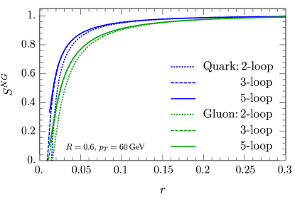
Figure 3: The non-global contribution to the soft function in eq. (30) for quark jets (blue) and gluon jets (green) with R=0.6 at pT=60subscript𝑝𝑇60p_{T}=60 GeV. Shown are the results up to two-loop (dotted), three-loop (dashed) and five-loop order (solid).

The leading NGLs in the hemisphere case are described by a universal function, where in our case the argument of the logarithm is R/r𝑅𝑟R/r. We will work in the large Ncsubscript𝑁𝑐N_{c} approximation (the leading NGLs without this approximation have been studied in ref. Hatta:2013iba ). Rather than using the fit of ref. Dasgupta:2001sh , we employ the solution to the BMS equation Banfi:2002hw up to five-loop order Schwartz:2014wha ,

SqNG(L^)=1π224L^2+ζ312L^3+π434560L^4+(π2ζ3360+17ζ5480)L^5+𝒪(L6),superscriptsubscript𝑆𝑞NG^𝐿1superscript𝜋224superscript^𝐿2subscript𝜁312superscript^𝐿3superscript𝜋434560superscript^𝐿4superscript𝜋2subscript𝜁336017subscript𝜁5480superscript^𝐿5𝒪superscript𝐿6\displaystyle S_{q}^{\rm NG}(\widehat{L})=1-\frac{\pi^{2}}{24}\widehat{L}^{2}+\frac{\zeta_{3}}{12}\widehat{L}^{3}+\frac{\pi^{4}}{34560}\widehat{L}^{4}+\Big{(}-\frac{\pi^{2}\zeta_{3}}{360}+\frac{17\zeta_{5}}{480}\Big{)}\widehat{L}^{5}+\mathcal{O}(L^{6})\,, (30)

where

L^=αsNcπlnRr.^𝐿subscript𝛼𝑠subscript𝑁𝑐𝜋𝑅𝑟\displaystyle\widehat{L}=\frac{\alpha_{s}N_{c}}{\pi}\ln\frac{R}{r}\,. (31)

The advantage of using this result is that it allows us to test the perturbative convergence, which is excellent for the range of r/R𝑟𝑅r/R we are interested in. Specifically, there is a small difference from including the cubic term in eq. (30), but the effect of subsequent terms is not visible, as is clear from fig. 3. This figure also shows that the effect of the non-global contribution to the soft function is limited to rather small values of r𝑟r. For the gluon case we have SgNG=(SqNG)2superscriptsubscript𝑆𝑔NGsuperscriptsuperscriptsubscript𝑆𝑞NG2S_{g}^{\rm NG}=(S_{q}^{\rm NG})^{2}, which follows from rewriting the adjoint Wilson line in terms of a fundamental and anti-fundamental Wilson line.777Alternatively, one can use non-abelian exponentation, and note that the webs only differ by a factor CFsubscript𝐶𝐹C_{F} vs. CAsubscript𝐶𝐴C_{A}, implying lnSgNG=(CA/CF)lnSqNG=ln(SqNG)2\ln S_{g}^{\rm NG}=(C_{A}/C_{F})\ln S_{q}^{\rm NG}=\ln(S_{q}^{\rm NG})^{2}, in the large NCsubscript𝑁𝐶N_{C} approximation. We thank D. Neill for discussions on this.

3 Collinear function including recoil

The definition of the collinear function is similar to eq. (2.1), and is given by the following expression for the quark case,

Cq(zr,pTr,k,μ,ν)subscript𝐶𝑞subscript𝑧𝑟subscript𝑝𝑇𝑟subscript𝑘perpendicular-to𝜇𝜈\displaystyle C_{q}(z_{r},p_{T}r,k_{\perp},\mu,\nu) (32)
=16π3X12NcTr[n¯/20|δ(2pTn¯𝒫)δ2(𝒫k)χn(0)|XX|χ¯n(0)|0]δ(zrpT(jr)pT).\displaystyle\quad=16\pi^{3}\,\sum_{X}\frac{1}{2N_{c}}\,{\rm Tr}\Big{[}\frac{\bar{n}\!\!\!/}{2}\langle 0|\delta(2p_{T}\!-\!\bar{n}\cdot{\mathcal{P}})\delta^{2}({\mathcal{P}}_{\perp}\!-\!k_{\perp})\chi_{n}(0)|X\rangle\langle X|\bar{\chi}_{n}(0)|0\rangle\Big{]}\delta\Big{(}z_{r}-\frac{p_{T}(j_{r})}{p_{T}}\Big{)}\,.

As before, we take the jet rapidity η𝜂\eta equal to zero, since the measurement is invariant under boosts along the beam axis. In contrast to eq. (2.1), all this collinear radiation is inside the jet, so there is no sum over jets in X𝑋X or measurement of z𝑧z. The recoil due to soft radiation is accounted for through the δ2(𝒫k)superscript𝛿2subscript𝒫perpendicular-tosubscript𝑘perpendicular-to\delta^{2}({\mathcal{P}}_{\perp}-k_{\perp}). At tree level, the collinear function is given by

Cd(zr,pTr,k,μ,ν)=δ(1zr)Θ(k<pTr),subscript𝐶𝑑subscript𝑧𝑟subscript𝑝𝑇𝑟subscript𝑘perpendicular-to𝜇𝜈𝛿1subscript𝑧𝑟Θsubscript𝑘perpendicular-tosubscript𝑝𝑇𝑟\displaystyle C_{d}(z_{r},p_{T}r,k_{\perp},\mu,\nu)=\delta(1-z_{r})\,\Theta(k_{\perp}<p_{T}r)\,, (33)

for both quarks (d=q𝑑𝑞d=q) and gluons (d=g𝑑𝑔d=g). This simply states that as long as the recoil is not too large (k<pTr)subscript𝑘perpendicular-tosubscript𝑝𝑇𝑟(k_{\perp}<p_{T}r), the parton is inside the cone of radius r𝑟r around the jet axis, and zr=1subscript𝑧𝑟1z_{r}=1.

In this section we calculate the collinear function at order αssubscript𝛼𝑠\alpha_{s}, which involves the collinear splitting of an initial quark or gluon into two partons. We give the collinear phase-space and matrix elements in sec. 3.1, and the geometry of the setup is described in sec. 3.2. The resulting integrals are performed in detail for the quark case in sec. 3.3, and results for the gluon case are presented in sec. 3.4. We verify in app. C that our result satisfies the rapidity renormalization group equation.

3.1 Collinear phase-space and matrix elements

Due to the recoil of the soft radiation, the jet axis is not aligned with the initial parton, requiring us to take the azimuthal dependence into account in the phase-space integration of the collinear-matrix elements,

dΦ2σ2,qcdifferential-dsubscriptΦ2subscriptsuperscript𝜎𝑐2𝑞\displaystyle\int\mathrm{d}\Phi_{2}\sigma^{c}_{2,q} =αs2π2(eγEμ2)ϵΓ(1ϵ)02πdϕ01dxP^qq(x)dqq1+2ϵ,absentsubscript𝛼𝑠2superscript𝜋2superscriptsuperscript𝑒subscript𝛾𝐸superscript𝜇2italic-ϵΓ1italic-ϵsuperscriptsubscript02𝜋differential-ditalic-ϕsuperscriptsubscript01differential-d𝑥subscript^𝑃𝑞𝑞𝑥dsubscript𝑞perpendicular-tosuperscriptsubscript𝑞perpendicular-to12italic-ϵ\displaystyle=\frac{\alpha_{s}}{2\pi^{2}}\frac{(e^{\gamma_{E}}\mu^{2})^{\epsilon}}{\Gamma(1-\epsilon)}\int_{0}^{2\pi}\mathrm{d\phi}\int_{0}^{1}\mathrm{d}x\;\hat{P}_{qq}(x)\int\frac{\mathrm{d}q_{\perp}}{q_{\perp}^{1+2\epsilon}},
dΦ2σ2,gcdifferential-dsubscriptΦ2subscriptsuperscript𝜎𝑐2𝑔\displaystyle\int\mathrm{d}\Phi_{2}\sigma^{c}_{2,g} =αs2π2(eγEμ2)ϵΓ(1ϵ)02πdϕ01dx[nfP^qg(x)+12P^gg(x)]dqq1+2ϵ.absentsubscript𝛼𝑠2superscript𝜋2superscriptsuperscript𝑒subscript𝛾𝐸superscript𝜇2italic-ϵΓ1italic-ϵsuperscriptsubscript02𝜋differential-ditalic-ϕsuperscriptsubscript01differential-d𝑥delimited-[]subscript𝑛𝑓subscript^𝑃𝑞𝑔𝑥12subscript^𝑃𝑔𝑔𝑥dsubscript𝑞perpendicular-tosuperscriptsubscript𝑞perpendicular-to12italic-ϵ\displaystyle=\frac{\alpha_{s}}{2\pi^{2}}\frac{(e^{\gamma_{E}}\mu^{2})^{\epsilon}}{\Gamma(1-\epsilon)}\int_{0}^{2\pi}\mathrm{d\phi}\int_{0}^{1}\mathrm{d}x\;\left[n_{f}\hat{P}_{qg}(x)+\frac{1}{2}\hat{P}_{gg}(x)\right]\int\frac{\mathrm{d}q_{\perp}}{q_{\perp}^{1+2\epsilon}}\,. (34)

Here dΦ2dsubscriptΦ2\mathrm{d}\Phi_{2} denotes the two-body collinear phase-space integration and σ2,qcsubscriptsuperscript𝜎𝑐2𝑞\sigma^{c}_{2,q} is the collinear matrix element squared. The two partons have transverse momentum qsubscript𝑞perpendicular-toq_{\perp} with respect to the initial parton and carry a fraction z𝑧z and 1z1𝑧1-z of its longitudinal momentum, whose distribution is described by the splitting functions888We introduce a hat to avoid potential confusion with the splitting functions given in eq. (2.1).

P^qq(x)subscript^𝑃𝑞𝑞𝑥\displaystyle\hat{P}_{qq}(x) =CF[1+x21xϵ(1x)],absentsubscript𝐶𝐹delimited-[]1superscript𝑥21𝑥italic-ϵ1𝑥\displaystyle=C_{F}\Big{[}\frac{1+x^{2}}{1-x}-\epsilon(1-x)\Big{]},
P^qg(x)subscript^𝑃𝑞𝑔𝑥\displaystyle\hat{P}_{qg}(x) =TF[12x(1x)+2ϵx(1x)],absentsubscript𝑇𝐹delimited-[]12𝑥1𝑥2italic-ϵ𝑥1𝑥\displaystyle=T_{F}\Big{[}1-2x(1-x)+2\epsilon\,x(1-x)\Big{]},
P^gg(x)subscript^𝑃𝑔𝑔𝑥\displaystyle\hat{P}_{gg}(x) =2CA[x1x+1xx+x(1x)].absent2subscript𝐶𝐴delimited-[]𝑥1𝑥1𝑥𝑥𝑥1𝑥\displaystyle=2C_{A}\Big{[}\frac{x}{1-x}+\frac{1-x}{x}+x(1-x)\Big{]}. (35)

We will make frequent use of the angles of the partons with respect to the initial parton,

β1=qxpT,β2=q(1x)pTformulae-sequencesubscript𝛽1subscript𝑞perpendicular-to𝑥subscript𝑝𝑇subscript𝛽2subscript𝑞perpendicular-to1𝑥subscript𝑝𝑇\displaystyle\beta_{1}=\frac{q_{\perp}}{xp_{T}}\,,\qquad\beta_{2}=\frac{q_{\perp}}{(1-x)p_{T}} (36)

where pTsubscript𝑝𝑇p_{T} is the transverse momentum of the jet.

3.2 Geometry of the measurement

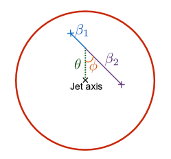
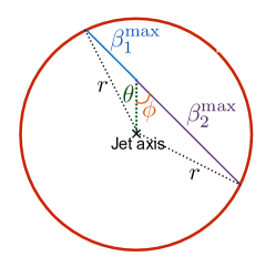
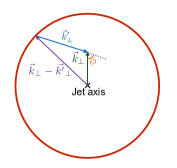
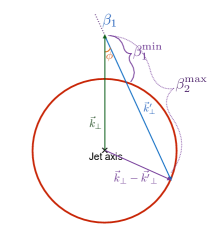
We now describe the geometry of the setup, starting with the case where the initial parton is inside the central subjet. Projecting the jet onto a plane perpendicular to the jet axis, as shown in the left panel of fig. 4, we can treat the polar angles as distances since r1much-less-than𝑟1r\ll 1. The central subjet corresponds to a circle of radius r𝑟r, and the recoil due to the total transverse momentum ksubscript𝑘perpendicular-tok_{\perp} of soft radiation in the jet corresponds to a displacement of the initial collinear parton by a distance θ=k/pT𝜃subscript𝑘perpendicular-tosubscript𝑝𝑇\theta=k_{\perp}/p_{T}. The angles βisubscript𝛽𝑖\beta_{i} also correspond to distances, though the azimuthal angle ϕitalic-ϕ\phi remains a true angle.

Refer to caption
Refer to caption

.

Figure 4: Projection of the central subjet of radius r𝑟r onto a plane perpendicular to the jet axis. θ𝜃\theta is the displacement due to recoil and is here assumed to be less than r𝑟r. In the left panel a splitting is shown. In the right panel βimaxsuperscriptsubscript𝛽𝑖max\beta_{i}^{\rm max} is shown, which is the upper bound on βisubscript𝛽𝑖\beta_{i} such that the corresponding parton lies inside the central subjet.

The condition for each of the partons produced by the splitting to be inside the central subjet is βiβ1maxsubscript𝛽𝑖superscriptsubscript𝛽1max\beta_{i}\leq\beta_{1}^{\rm max}, displayed in the right panel of fig. 4. Some trigonometry yields

β1,2maxsuperscriptsubscript𝛽12max\displaystyle\beta_{1,2}^{\rm max} =r1+θ2r22θr(±cosϕ1θ2r2sin2ϕ+θrsin2ϕ),absent𝑟1superscript𝜃2superscript𝑟22𝜃𝑟plus-or-minusitalic-ϕ1superscript𝜃2superscript𝑟2superscript2italic-ϕ𝜃𝑟superscript2italic-ϕ\displaystyle=r\sqrt{1+\frac{\theta^{2}}{r^{2}}-2\frac{\theta}{r}\biggl{(}\pm\cos\phi\,\sqrt{1-\frac{\theta^{2}}{r^{2}}\sin^{2}\phi}+\frac{\theta}{r}\sin^{2}\phi\biggr{)}}, (37)

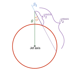
The case θ>r𝜃𝑟\theta>r, where the initial parton is outside of the jet, requires the setup depicted in fig. 5. Here only one parton produced in the splitting can be inside the central subjet, and there is a minimum and maximum value for βisubscript𝛽𝑖\beta_{i}. For parton 2,

β2min,max=θ[cosϕr2θ2sin2ϕ],superscriptsubscript𝛽2minmax𝜃delimited-[]minus-or-plusitalic-ϕsuperscript𝑟2superscript𝜃2superscript2italic-ϕ\displaystyle\beta_{2}^{{\rm min},{\rm max}}=\theta\biggl{[}\cos\phi\mp\sqrt{\frac{r^{2}}{\theta^{2}}-\sin^{2}\phi}\,\biggr{]}\,, (38)

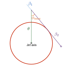
and the expressions for β1min,maxsuperscriptsubscript𝛽1minmax\beta_{1}^{{\rm min},{\rm max}} can be obtained by substituting ϕϕ+πitalic-ϕitalic-ϕ𝜋\phi\rightarrow\phi+\pi. These expressions are not valid for all ϕitalic-ϕ\phi, breaking down when the square root becomes imaginary. The maximum ϕitalic-ϕ\phi is shown in the right panel of fig. 5, and leads to the following boundaries

parton 1: πϕmax𝜋subscriptitalic-ϕmax\displaystyle\quad\pi-\phi_{\rm max} <ϕ<π+ϕmax,absentitalic-ϕ𝜋subscriptitalic-ϕmax\displaystyle<\phi<\pi+\phi_{\rm max}\,, ϕmaxsubscriptitalic-ϕmax\displaystyle\phi_{\rm max} =arcsin(rθ)absent𝑟𝜃\displaystyle=\arcsin\Bigl{(}\frac{r}{\theta}\Bigr{)}
parton 2: ϕmaxsubscriptitalic-ϕmax\displaystyle\quad-\phi_{\rm max} <ϕ<ϕmax.absentitalic-ϕsubscriptitalic-ϕmax\displaystyle<\phi<\phi_{\rm max}\,. (39)
Refer to caption
Refer to caption

.

Figure 5: Geometry of the central subjet when the recoil θ𝜃\theta is larger than the radius r𝑟r. In the left panel the minimum and maximum values of β2subscript𝛽2\beta_{2} are shown such that this parton is inside the central subjet. The right panel depicts the maximum value of ϕitalic-ϕ\phi.

3.3 Integrals for the quark collinear function

We now present the calculation of the collinear function for an initiating quark, separating the two cases:

Cq(1)(zr,pTr,k,μ,ν)=Θ(k<pTr)Cq(θ<r)+Θ(k>pTr)Cq(θ>r).subscriptsuperscript𝐶1𝑞subscript𝑧𝑟subscript𝑝𝑇𝑟subscript𝑘perpendicular-to𝜇𝜈Θsubscript𝑘perpendicular-tosubscript𝑝𝑇𝑟superscriptsubscript𝐶𝑞𝜃𝑟Θsubscript𝑘perpendicular-tosubscript𝑝𝑇𝑟superscriptsubscript𝐶𝑞𝜃𝑟\displaystyle C^{(1)}_{q}(z_{r},p_{T}r,k_{\perp},\mu,\nu)=\Theta(k_{\perp}<p_{T}r)\,C_{q}^{(\theta<r)}+\Theta(k_{\perp}>p_{T}r)\,C_{q}^{(\theta>r)}. (40)

In the first case

Cq(θ<r)superscriptsubscript𝐶𝑞𝜃𝑟\displaystyle C_{q}^{(\theta<r)} =(A)θ<r+(B)θ<r+(C)θ<r,absentsubscriptA𝜃rsubscriptB𝜃rsubscriptC𝜃r\displaystyle=(\rm A)_{\theta<r}+(\rm B)_{\theta<r}+(\rm C)_{\theta<r}\,,
(A)θ<rsubscriptA𝜃r\displaystyle(\rm A)_{\theta<r} =δ(1zr)dΦ2σ2,qcΘ(β1<β1max)Θ(β2<β2max),absent𝛿1subscript𝑧𝑟differential-dsubscriptΦ2subscriptsuperscript𝜎𝑐2𝑞Θsubscript𝛽1subscriptsuperscript𝛽max1Θsubscript𝛽2subscriptsuperscript𝛽max2\displaystyle=\delta(1-z_{r})\int\!\mathrm{d}\Phi_{2}\,\sigma^{c}_{2,q}\,\Theta(\beta_{1}<\beta^{\rm max}_{1})\Theta(\beta_{2}<\beta^{\rm max}_{2})\,,
(B)θ<rsubscriptB𝜃r\displaystyle(\rm B)_{\theta<r} =dΦ2σ2,qcδ(xzr)Θ(β1<β1max)Θ(β2>β2max),absentdifferential-dsubscriptΦ2subscriptsuperscript𝜎𝑐2𝑞𝛿𝑥subscript𝑧𝑟Θsubscript𝛽1subscriptsuperscript𝛽max1Θsubscript𝛽2subscriptsuperscript𝛽max2\displaystyle=\int\!\mathrm{d}\Phi_{2}\,\sigma^{c}_{2,q}\,\delta(x-z_{r})\,\Theta(\beta_{1}<\beta^{\rm max}_{1})\Theta(\beta_{2}>\beta^{\rm max}_{2})\,,
(C)θ<rsubscriptC𝜃r\displaystyle(\rm C)_{\theta<r} =dΦ2σ2,qcδ(1xzr)Θ(β1>β1max)Θ(β2<β2max),absentdifferential-dsubscriptΦ2subscriptsuperscript𝜎𝑐2𝑞𝛿1𝑥subscript𝑧𝑟Θsubscript𝛽1subscriptsuperscript𝛽𝑚𝑎𝑥1Θsubscript𝛽2subscriptsuperscript𝛽𝑚𝑎𝑥2\displaystyle=\int\!\mathrm{d}\Phi_{2}\,\sigma^{c}_{2,q}\,\delta(1-x-z_{r})\,\Theta(\beta_{1}>\beta^{max}_{1})\Theta(\beta_{2}<\beta^{max}_{2}), (41)

where (A) refers to the case when both partons end up inside the subjet, (B) when only parton 1 (quark) ends up inside and (C) when only parton 2 (gluon) does (using the same labels as in ref. Kang:2017mda ). In the second case only one parton can be inside the subjet, and

Cq(θ>r)superscriptsubscript𝐶𝑞𝜃𝑟\displaystyle C_{q}^{(\theta>r)} =(B)θ>r+(C)θ>r,absentsubscriptB𝜃rsubscriptC𝜃r\displaystyle=(\rm B)_{\theta>r}+(\rm C)_{\theta>r}\,,
(B)θ>rsubscriptB𝜃𝑟\displaystyle({\rm B})_{\theta>r} =dΦ2σ2,qcδ(xzr)Θ(πϕmax<ϕ<π+ϕmax)Θ(β1min<β1<β1max),absentdifferential-dsubscriptΦ2subscriptsuperscript𝜎𝑐2𝑞𝛿𝑥subscript𝑧𝑟Θ𝜋subscriptitalic-ϕmaxitalic-ϕ𝜋subscriptitalic-ϕmaxΘsuperscriptsubscript𝛽1minsubscript𝛽1superscriptsubscript𝛽1max\displaystyle=\int\!\mathrm{d}\Phi_{2}\,\sigma^{c}_{2,q}\,\delta(x-z_{r})\,\Theta(\pi-\phi_{\rm max}<\phi<\pi+\phi_{\rm max})\,\Theta(\beta_{1}^{\rm min}<\beta_{1}<\beta_{1}^{\rm max})\,,
(C)θ>rsubscriptC𝜃𝑟\displaystyle({\rm C})_{\theta>r} =dΦ2σ2,qcδ(1xzr)Θ(ϕmax<ϕ<ϕmax)Θ(β2min<β2<β2max).absentdifferential-dsubscriptΦ2subscriptsuperscript𝜎𝑐2𝑞𝛿1𝑥subscript𝑧𝑟Θsubscriptitalic-ϕmaxitalic-ϕsubscriptitalic-ϕmaxΘsuperscriptsubscript𝛽2minsubscript𝛽2superscriptsubscript𝛽2max\displaystyle=\int\!\mathrm{d}\Phi_{2}\,\sigma^{c}_{2,q}\,\delta(1-x-z_{r})\,\Theta(-\phi_{\rm max}<\phi<\phi_{\rm max})\,\Theta(\beta_{2}^{\rm min}<\beta_{2}<\beta_{2}^{\rm max})\,. (42)

The contribution where neither parton is inside is irrelevant, since then zr=0subscript𝑧𝑟0z_{r}=0.

We now set out to calculate these integrals. For (A)θ<r we use eq. (36) to rewrite the x𝑥x integral and ΘΘ\Theta functions

01dxΘ(β1<β1max)Θ(β2<β2max)superscriptsubscript01differential-d𝑥Θsubscript𝛽1subscriptsuperscript𝛽max1Θsubscript𝛽2subscriptsuperscript𝛽max2\displaystyle\int_{0}^{1}\!\mathrm{d}x\,\Theta(\beta_{1}<\beta^{\rm max}_{1})\Theta(\beta_{2}<\beta^{\rm max}_{2}) =01dxΘ(q<xpTβ1max)Θ(q<(1x)pTβ2max)absentsuperscriptsubscript01differential-d𝑥Θsubscript𝑞perpendicular-to𝑥subscript𝑝𝑇superscriptsubscript𝛽1maxΘsubscript𝑞perpendicular-to1𝑥subscript𝑝𝑇superscriptsubscript𝛽2max\displaystyle=\int_{0}^{1}\!\mathrm{d}x\,\Theta(q_{\perp}<xp_{T}\beta_{1}^{\rm max})\,\Theta(q_{\perp}<(1-x)p_{T}\beta_{2}^{\rm max})
=0β~dxΘ(q<xpTβ1max)absentsuperscriptsubscript0~𝛽differential-d𝑥Θsubscript𝑞perpendicular-to𝑥subscript𝑝𝑇superscriptsubscript𝛽1max\displaystyle=\int_{0}^{\widetilde{\beta}}\!\mathrm{d}x\,\Theta(q_{\perp}<xp_{T}\beta_{1}^{\rm max})
+β~1dxΘ(q<(1x)pTβ2max),superscriptsubscript~𝛽1differential-d𝑥Θsubscript𝑞perpendicular-to1𝑥subscript𝑝𝑇superscriptsubscript𝛽2max\displaystyle\quad+\int_{\widetilde{\beta}}^{1}\!\mathrm{d}x\,\Theta(q_{\perp}<(1-x)p_{T}\beta_{2}^{\rm max}), (43)

where β~~𝛽\widetilde{\beta} with 0<β~<10~𝛽10<\widetilde{\beta}<1 is given by

β~=β2maxβ1max+β2max.~𝛽superscriptsubscript𝛽2maxsuperscriptsubscript𝛽1maxsuperscriptsubscript𝛽2max\displaystyle\widetilde{\beta}=\frac{\beta_{2}^{\rm max}}{\beta_{1}^{\rm max}+\beta_{2}^{\rm max}}\,. (44)

Inserting this in eq. (3.3), and performing the x𝑥x and qsubscript𝑞perpendicular-toq_{\perp} integrals, we obtain

(A)θ<rsubscript𝐴𝜃𝑟\displaystyle(A)_{\theta<r} =αsCF2π2δ(1zr)02πdϕ{12ϵ2+1ϵ(L22+34)+L224+3L24ln2(1β~)\displaystyle=\frac{\alpha_{s}C_{F}}{2\pi^{2}}\,\delta(1-z_{r})\int_{0}^{2\pi}\mathrm{d\phi}\bigg{\{}\frac{1}{2\epsilon^{2}}+\frac{1}{\epsilon}\Big{(}\frac{L_{2}}{2}+\frac{3}{4}\Big{)}+\frac{L_{2}^{2}}{4}+\frac{3L_{2}}{4}-\ln^{2}(1-\widetilde{\beta})
+2lnβ~ln(1β~)32ln(1β~)+2Li2(1β~)β~2+23π28},\displaystyle\quad+2\ln\widetilde{\beta}\ln(1-\widetilde{\beta})-\frac{3}{2}\ln(1-\widetilde{\beta})+2\text{Li}_{2}\bigl{(}1-\widetilde{\beta}\bigr{)}-\frac{\widetilde{\beta}}{2}+2-\frac{3\pi^{2}}{8}\bigg{\}}, (45)

in terms of Lisubscript𝐿𝑖L_{i} defined as

Li=ln(μ2pT2(βimax)2).subscript𝐿𝑖superscript𝜇2superscriptsubscript𝑝𝑇2superscriptsuperscriptsubscript𝛽𝑖max2\displaystyle L_{i}=\ln\bigg{(}\frac{\mu^{2}}{p_{T}^{2}(\beta_{i}^{\rm max})^{2}}\bigg{)}\,. (46)

We cannot perform the integral over ϕitalic-ϕ\phi analytically, as it involves the rather complicated expression in eq. (37). However, this is not a problem as we have already isolated the divergences.

The calculation of (B)θ<r involves rapidity divergences, which we regulate using the η𝜂\eta regulator, resulting in

(B)θ<rsubscriptB𝜃𝑟\displaystyle({\rm B})_{\theta<r} =αsCF2π2eϵγEΓ(1ϵ)μ2ϵ02πdϕβ~1dxδ(xzr)[1+x21xϵ(1x)][ν2(1x)pT]ηabsentsubscript𝛼𝑠subscript𝐶𝐹2superscript𝜋2superscript𝑒italic-ϵsubscript𝛾𝐸Γ1italic-ϵsuperscript𝜇2italic-ϵsuperscriptsubscript02𝜋differential-ditalic-ϕsuperscriptsubscript~𝛽1differential-d𝑥𝛿𝑥subscript𝑧𝑟delimited-[]1superscript𝑥21𝑥italic-ϵ1𝑥superscriptdelimited-[]𝜈21𝑥subscript𝑝𝑇𝜂\displaystyle=\frac{\alpha_{s}C_{F}}{2\pi^{2}}\,\frac{e^{\epsilon\gamma_{E}}}{\Gamma(1-\epsilon)}\,\mu^{2\epsilon}\,\int_{0}^{2\pi}\!\mathrm{d}\phi\int_{\widetilde{\beta}}^{1}\mathrm{d}x\,\delta(x-z_{r})\Big{[}\frac{1+x^{2}}{1-x}-\epsilon(1-x)\Big{]}\Big{[}\frac{\nu}{2(1-x)p_{T}}\Big{]}^{\eta}
×(1x)pTβ2maxxpTβ1maxdqq1+2ϵ\displaystyle\quad\times\int^{xp_{T}\beta_{1}^{\rm max}}_{(1-x)p_{T}\beta_{2}^{\rm max}}\frac{\mathrm{d}q_{\perp}}{q_{\perp}^{1+2\epsilon}}
=αsCF2π202πdϕ{δ(1zr)[1η(1ϵ+L1)12ϵ2+1ϵ(LνL22)+LνL1L224+π224]\displaystyle=\frac{\alpha_{s}C_{F}}{2\pi^{2}}\int_{0}^{2\pi}\!\mathrm{d}\phi\,\bigg{\{}\delta(1-z_{r})\bigg{[}\frac{1}{\eta}\Big{(}\frac{1}{\epsilon}+L_{1}\Big{)}-\frac{1}{2\epsilon^{2}}+\frac{1}{\epsilon}\,\Big{(}L_{\nu}-\frac{L_{2}}{2}\Big{)}+L_{\nu}L_{1}-\frac{L_{2}^{2}}{4}+\frac{\pi^{2}}{24}\bigg{]}
+Θ(zr>β~)[(1+zr2)(ln(1zr)1zr)+ln(β~1β~)1+zr2(1zr)++(1+zr2)lnzr1zr]}.\displaystyle\quad+\Theta\big{(}z_{r}>\widetilde{\beta}\big{)}\bigg{[}-(1+z_{r}^{2})\bigg{(}\frac{\ln(1\!-\!z_{r})}{1-z_{r}}\bigg{)}_{\!\!+}-\ln\bigg{(}\frac{\widetilde{\beta}}{1-\widetilde{\beta}}\bigg{)}\frac{1+z_{r}^{2}}{(1-z_{r})}_{+}+\frac{(1+z_{r}^{2})\ln z_{r}}{1-z_{r}}\bigg{]}\bigg{\}}. (47)

where Lνsubscript𝐿𝜈L_{\nu} is defined as

Lν=lnν2pT.subscript𝐿𝜈𝜈2subscript𝑝𝑇\displaystyle L_{\nu}=\ln\frac{\nu}{2p_{T}}\,. (48)

Performing a similar calculation for (C)θ<r we obtain

(C)θ<r=αs2π202πdϕΘ(zr>1β~){Pgq(zr)[ln(zr1zr)+ln(β~1β~)]}.subscriptC𝜃𝑟subscript𝛼𝑠2superscript𝜋2superscriptsubscript02𝜋differential-ditalic-ϕΘsubscript𝑧𝑟1~𝛽subscript𝑃𝑔𝑞subscript𝑧𝑟delimited-[]subscript𝑧𝑟1subscript𝑧𝑟~𝛽1~𝛽\displaystyle({\rm C})_{\theta<r}=\frac{\alpha_{s}}{2\pi^{2}}\int_{0}^{2\pi}\!\mathrm{d}\phi\,\Theta\big{(}z_{r}>1-\widetilde{\beta}\big{)}\biggl{\{}P_{gq}(z_{r})\biggl{[}\ln\biggl{(}\frac{z_{r}}{1-z_{r}}\biggr{)}+\ln\biggl{(}\frac{\widetilde{\beta}}{1-\widetilde{\beta}}\biggr{)}\biggr{]}\biggr{\}}\,. (49)

Note that the factor CFsubscript𝐶𝐹C_{F} is inside the Pgqsubscript𝑃𝑔𝑞P_{gq} splitting function, which was defined in eq. (2.1).

Moving on to the case θ>r𝜃𝑟\theta>r, we also have to regulate rapidity divegences for (B)θ>rsubscript𝐵𝜃𝑟(B)_{\theta>r},

(B)θ>r=subscriptB𝜃𝑟absent\displaystyle({\rm B})_{\theta>r}= αsCF2π2eϵγEΓ(1ϵ)μ2ϵπϕmaxπ+ϕmaxdϕ01dxδ(xzr)[1+x21xϵ(1x)](ν2(1x)pT)ηsubscript𝛼𝑠subscript𝐶𝐹2superscript𝜋2superscript𝑒italic-ϵsubscript𝛾𝐸Γ1italic-ϵsuperscript𝜇2italic-ϵsuperscriptsubscript𝜋subscriptitalic-ϕmax𝜋subscriptitalic-ϕmaxdifferential-ditalic-ϕsuperscriptsubscript01differential-d𝑥𝛿𝑥subscript𝑧𝑟delimited-[]1superscript𝑥21𝑥italic-ϵ1𝑥superscript𝜈21𝑥subscript𝑝𝑇𝜂\displaystyle\frac{\alpha_{s}C_{F}}{2\pi^{2}}\,\frac{e^{\epsilon\gamma_{E}}}{\Gamma(1-\epsilon)}\,\mu^{2\epsilon}\int_{\pi-\phi_{\rm max}}^{\pi+\phi_{\rm max}}\!\mathrm{d}\phi\int_{0}^{1}\!\mathrm{d}x\,\delta(x-z_{r})\Bigl{[}\frac{1+x^{2}}{1-x}-\epsilon(1-x)\Bigr{]}\Bigl{(}\frac{\nu}{2(1-x)p_{T}}\Bigr{)}^{\eta}
×xpTβ1minxpTβ1maxdqq1+2ϵ\displaystyle\times\int^{xp_{T}\beta_{1}^{\rm max}}_{xp_{T}\beta_{1}^{\rm min}}\frac{\mathrm{d}q_{\perp}}{q_{\perp}^{1+2\epsilon}}
=αsCF2π2[δ(1zr)(2η+2Lν)1+zr2(1zr)+]ϕmaxϕmaxdϕln(β2minβ2max)absentsubscript𝛼𝑠subscript𝐶𝐹2superscript𝜋2delimited-[]𝛿1subscript𝑧𝑟2𝜂2subscript𝐿𝜈subscript1superscriptsubscript𝑧𝑟21subscript𝑧𝑟superscriptsubscriptsubscriptitalic-ϕmaxsubscriptitalic-ϕmaxdifferential-ditalic-ϕsuperscriptsubscript𝛽2minsuperscriptsubscript𝛽2max\displaystyle=\frac{\alpha_{s}C_{F}}{2\pi^{2}}\,\biggl{[}\delta(1-z_{r})\Big{(}\frac{2}{\eta}+2L_{\nu}\Big{)}-\frac{1+z_{r}^{2}}{(1-z_{r})}_{+}\biggr{]}\int_{-\phi_{\rm max}}^{\phi_{\rm max}}\mathrm{d}\phi\ln\biggl{(}\frac{\beta_{2}^{\rm min}}{\beta_{2}^{\rm max}}\biggr{)} (50)

Note that we changed the ϕitalic-ϕ\phi integration region, which is why the final expression involves β2min,maxsuperscriptsubscript𝛽2minmax\beta_{2}^{\rm min,\,max} rather than β1min,maxsuperscriptsubscript𝛽1minmax\beta_{1}^{\rm min,\,max}. An analogous computation for (C)θ>r yields

(C)θ>r=αs2π2Pgq(zr)ϕmaxϕmaxdϕln(β2minβ2max).subscriptC𝜃𝑟subscript𝛼𝑠2superscript𝜋2subscript𝑃𝑔𝑞subscript𝑧𝑟superscriptsubscriptsubscriptitalic-ϕmaxsubscriptitalic-ϕmaxdifferential-ditalic-ϕsuperscriptsubscript𝛽2minsuperscriptsubscript𝛽2max\displaystyle({\rm C})_{\theta>r}=-\frac{\alpha_{s}}{2\pi^{2}}\,P_{gq}(z_{r})\int_{-\phi_{\rm max}}^{\phi_{\rm max}}\!\mathrm{d}\phi\ln\biggl{(}\frac{\beta_{2}^{\rm min}}{\beta_{2}^{\rm max}}\biggr{)}. (51)

Adding up all the contributions,

Cq(θ<r)superscriptsubscript𝐶𝑞𝜃𝑟\displaystyle C_{q}^{(\theta<r)} =αsCF2π202πdϕ{δ(1zr)[1η(1ϵ+L1)+1ϵ(Lν+34)+LνL1+3L14\displaystyle=\frac{\alpha_{s}C_{F}}{2\pi^{2}}\int_{0}^{2\pi}\!\mathrm{d}\phi\,\biggl{\{}\delta(1-z_{r})\bigg{[}\frac{1}{\eta}\Big{(}\frac{1}{\epsilon}+L_{1}\Big{)}+\frac{1}{\epsilon}\Big{(}L_{\nu}+\frac{3}{4}\Big{)}+L_{\nu}L_{1}+\frac{3L_{1}}{4} (52)
ln2(1β~)+2lnβ~ln(1β~)32lnβ~+2Li2(1β~)β~2π23+2]\displaystyle\quad-\ln^{2}(1-\widetilde{\beta})+2\ln\widetilde{\beta}\ln(1-\widetilde{\beta})-\frac{3}{2}\ln\widetilde{\beta}+2{\rm Li}_{2}(1-\widetilde{\beta})-\frac{\widetilde{\beta}}{2}-\frac{\pi^{2}}{3}+2\bigg{]}
+Θ(zr>β~)[(1+zr2)(ln(1zr)1zr)++ln(zr(1β~)β~)1+zr2(1zr)+]Θsubscript𝑧𝑟~𝛽delimited-[]1superscriptsubscript𝑧𝑟2subscript1subscript𝑧𝑟1subscript𝑧𝑟subscript𝑧𝑟1~𝛽~𝛽subscript1superscriptsubscript𝑧𝑟21subscript𝑧𝑟\displaystyle\quad+\Theta(z_{r}>\widetilde{\beta})\biggl{[}-(1+z_{r}^{2})\bigg{(}\frac{\ln(1-z_{r})}{1-z_{r}}\bigg{)}_{\!\!+}+\ln\biggl{(}\frac{z_{r}(1-\widetilde{\beta})}{\widetilde{\beta}}\biggr{)}\frac{1+z_{r}^{2}}{(1-z_{r})}_{+}\biggr{]}
+Θ(zr>1β~)[1+(1zr)2zrln(zrβ~(1zr)(1β~))]},\displaystyle\quad+\Theta(z_{r}>1-\widetilde{\beta})\biggl{[}\frac{1+(1-z_{r})^{2}}{z_{r}}\,\ln\biggl{(}\frac{z_{r}\widetilde{\beta}}{(1-z_{r})(1-\widetilde{\beta})}\biggr{)}\biggr{]}\biggr{\}},
Cq(θ>r)superscriptsubscript𝐶𝑞𝜃𝑟\displaystyle C_{q}^{(\theta>r)} =αsCF2π2[δ(1zr)(2η+2Lν)1+zr2(1zr)+1+(1zr)2zr]ϕmaxϕmaxdϕln(β2minβ2max),absentsubscript𝛼𝑠subscript𝐶𝐹2superscript𝜋2delimited-[]𝛿1subscript𝑧𝑟2𝜂2subscript𝐿𝜈subscript1superscriptsubscript𝑧𝑟21subscript𝑧𝑟1superscript1subscript𝑧𝑟2subscript𝑧𝑟superscriptsubscriptsubscriptitalic-ϕmaxsubscriptitalic-ϕmaxdifferential-ditalic-ϕsuperscriptsubscript𝛽2minsuperscriptsubscript𝛽2max\displaystyle=\frac{\alpha_{s}C_{F}}{2\pi^{2}}\biggl{[}\delta(1-z_{r})\Bigl{(}\frac{2}{\eta}+2L_{\nu}\Bigr{)}-\frac{1+z_{r}^{2}}{(1-z_{r})}_{+}-\frac{1+(1-z_{r})^{2}}{z_{r}}\biggr{]}\int_{-\phi_{\rm max}}^{\phi_{\rm max}}\!\mathrm{d}\phi\ln\left(\frac{\beta_{2}^{\rm min}}{\beta_{2}^{\rm max}}\right),

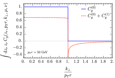
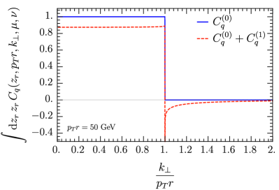
For the jet shape we only need the linear zrsubscript𝑧𝑟z_{r} moment (dzrzrdifferential-dsubscript𝑧𝑟subscript𝑧𝑟\int\mathrm{d}z_{r}\,z_{r}) of the collinear function, which we plot for quark jets in the left panel of fig. 6. The result depends on k/(pTr)subscript𝑘perpendicular-tosubscript𝑝𝑇𝑟k_{\perp}/(p_{T}r), shown on the horizontal axis, and on pTrsubscript𝑝𝑇𝑟p_{T}r, through the scale in αssubscript𝛼𝑠\alpha_{s}. First we note that the one-loop corrections are of order 10%, as is typical. At tree level there is a single collinear particle that is simply inside the jet if the recoil due to soft radiation is not too large, k<pTrsubscript𝑘perpendicular-tosubscript𝑝𝑇𝑟k_{\perp}<p_{T}r. One-loop corrections allow for nonzero values of the collinear function for larger values of ksubscript𝑘perpendicular-tok_{\perp}. That the collinear function attains a negative value is not a concern, since it does not correspond to a physical quantity (indeed, this depends on our choice of μ𝜇\mu and ν𝜈\nu-scales). We also note that the divergence at k=pTrsubscript𝑘perpendicular-tosubscript𝑝𝑇𝑟k_{\perp}=p_{T}r from one-loop corrections is integrable.
Refer to caption
Refer to caption

.

Figure 6: The linear zrsubscript𝑧𝑟z_{r} moment of the collinear function for quark jets (left) and gluon jets (right) at tree level (blue) and including one-loop corrections (red dashed), evaluated at the scales μ=pTr𝜇subscript𝑝𝑇𝑟\mu=p_{T}r and ν=pT𝜈subscript𝑝𝑇\nu=p_{T}.

3.4 Gluon collinear function

The calculation of the collinear function for gluons follows very similar steps. Splitting the calculation into the θ<r𝜃𝑟\theta<r and θ>r𝜃𝑟\theta>r contribution, we obtain

Cg(θ<r)superscriptsubscript𝐶𝑔𝜃𝑟\displaystyle C_{g}^{(\theta<r)} =αs2π202πdϕ(δ(1zr){CA[1η(1ϵ+L14+L24)+1ϵ(Lν+1112)\displaystyle=\frac{\alpha_{s}}{2\pi^{2}}\int_{0}^{2\pi}\mathrm{d\phi}\bigg{(}\delta(1-z_{r})\bigg{\{}C_{A}\bigg{[}\frac{1}{\eta}\Big{(}\frac{1}{\epsilon}+\frac{L_{1}}{4}+\frac{L_{2}}{4}\Big{)}+\frac{1}{\epsilon}\Big{(}L_{\nu}+\frac{11}{12}\Big{)}
+(Lν2+1124)(L1+L2)12ln21β~β~1112ln(β~(1β~))+16β~(1β~)subscript𝐿𝜈21124subscript𝐿1subscript𝐿212superscript21~𝛽~𝛽1112~𝛽1~𝛽16~𝛽1~𝛽\displaystyle\quad+\Big{(}\frac{L_{\nu}}{2}+\frac{11}{24}\Big{)}(L_{1}+L_{2})-\frac{1}{2}\ln^{2}\frac{1-\widetilde{\beta}}{\widetilde{\beta}}-\frac{11}{12}\ln\big{(}\widetilde{\beta}(1-\widetilde{\beta})\big{)}+\frac{1}{6}\widetilde{\beta}(1-\widetilde{\beta})
π26+6736]+nfTF[13ϵ16(L1+L2)+13ln(β~(1β~))13β~(1β~)59]}\displaystyle\quad-\frac{\pi^{2}}{6}+\frac{67}{36}\bigg{]}+n_{f}T_{F}\bigg{[}-\frac{1}{3\epsilon}-\frac{1}{6}(L_{1}+L_{2})+\frac{1}{3}\ln\big{(}\widetilde{\beta}(1-\widetilde{\beta})\big{)}-\frac{1}{3}\widetilde{\beta}(1-\widetilde{\beta})-\frac{5}{9}\bigg{]}\bigg{\}}
+Θ(zr>β~){CA(1zr+zr2)2zr(ln(1zr)1zr)++CA(1zr+zr2)2zr(1zr)+ln(zr(1β~)β~)\displaystyle\quad+\Theta(z_{r}>\widetilde{\beta})\bigg{\{}-C_{A}\frac{(1\!-\!z_{r}\!+\!z_{r}^{2})^{2}}{z_{r}}\bigg{(}\frac{\ln(1\!-\!z_{r})}{1-z_{r}}\bigg{)}_{+}\!\!+C_{A}\frac{(1\!-\!z_{r}\!+\!z_{r}^{2})^{2}}{z_{r}(1-z_{r})_{+}}\ln\bigg{(}\frac{z_{r}(1-\widetilde{\beta})}{\widetilde{\beta}}\bigg{)}
+nfTF(zr2+(1zr)2)ln(zr(1β~)(1zr)β~)}),\displaystyle\quad+n_{f}T_{F}(z_{r}^{2}+(1-z_{r})^{2})\ln\bigg{(}\frac{z_{r}(1\!-\!\widetilde{\beta})}{(1-z_{r})\widetilde{\beta}}\bigg{)}\bigg{\}}\bigg{)}\,,
Cg(θ>r)superscriptsubscript𝐶𝑔𝜃𝑟\displaystyle C_{g}^{(\theta>r)} =αs2π2{2CA[δ(1zr)(1η+Lν)(1zr+zr2)2zr(1zr)+]\displaystyle=\frac{\alpha_{s}}{2\pi^{2}}\bigg{\{}2C_{A}\bigg{[}\delta(1-z_{r})\Big{(}\frac{1}{\eta}+L_{\nu}\Big{)}-\frac{(1-z_{r}+z_{r}^{2})^{2}}{z_{r}(1-z_{r})_{+}}\bigg{]}
2nfTF(zr2+(1zr)2)}ϕmaxϕmaxdϕln(β2minβ2max).\displaystyle\quad-2n_{f}T_{F}(z_{r}^{2}+(1-z_{r})^{2})\bigg{\}}\int_{-\phi_{\rm max}}^{\phi_{\rm max}}\mathrm{d\phi}\ln\bigg{(}\frac{\beta_{2}^{\rm min}}{\beta_{2}^{\rm max}}\bigg{)}\,. (53)

The linear moment of the gluon collinear function is shown in the right panel of fig. 6. Its features are similar to that for quark jets (left panel), except that the one-loop corrections are larger due to the larger color factor (CAsubscript𝐶𝐴C_{A} vs. CFsubscript𝐶𝐹C_{F}).

4 Implementation and first results

This section describes how we implement our formulae to obtain numerical predictions. In sec. 4.1 our central scale choice is discussed. We then describe how we match our formulae for rRmuch-less-than𝑟𝑅r\ll R and rRless-than-or-similar-to𝑟𝑅r\lesssim R in sec. 4.2. The scale variations used to assess the perturbative uncertainty are given in sec. 4.3. We conclude in sec. 4.4 with some first, purely perturbative, results for the jet shape for quark and gluons jets.

4.1 Central scale choice

We start by discussing the scales for the regime rRless-than-or-similar-to𝑟𝑅r\lesssim R, described by the factorization in eq. (2.1). We take

μ=pT,μ𝒢=pTR,formulae-sequencesubscript𝜇subscript𝑝𝑇subscript𝜇𝒢subscript𝑝𝑇𝑅\displaystyle\mu_{\cal H}=p_{T}\,,\qquad\mu_{{\mathcal{G}}}=p_{T}R\,, (54)

as our central scale choice. In the regime rRmuch-less-than𝑟𝑅r\ll R, 𝒢𝒢{\mathcal{G}} is refactorized in terms of hard, collinear and soft functions, see eq. (12). We will take as their central scales

μsubscript𝜇\displaystyle\mu_{\cal H} =pT,absentsubscript𝑝𝑇\displaystyle=p_{T}\,, μHsubscript𝜇𝐻\displaystyle\mu_{H} =pTR,absentsubscript𝑝𝑇𝑅\displaystyle=p_{T}R\,, μCsubscript𝜇𝐶\displaystyle\mu_{C} =pTr,absentsubscript𝑝𝑇𝑟\displaystyle=p_{T}r\,, μSsubscript𝜇𝑆\displaystyle\mu_{S} =pTr,absentsubscript𝑝𝑇𝑟\displaystyle=p_{T}r\,,
νCsubscript𝜈𝐶\displaystyle\nu_{C} =pT,absentsubscript𝑝𝑇\displaystyle=p_{T}\,, νSsubscript𝜈𝑆\displaystyle\nu_{S} =1bR.absent1subscript𝑏perpendicular-to𝑅\displaystyle=\frac{1}{b_{\perp}R}\,. (55)

We deviate from eq. (2.1) by expressing νSsubscript𝜈𝑆\nu_{S} in terms of bsubscript𝑏perpendicular-tob_{\perp}, which is the Fourier conjugate variable of ksubscript𝑘perpendicular-tok_{\perp} (not pTsubscript𝑝𝑇p_{T}). Since collinear and soft modes contribute to ksubscript𝑘perpendicular-tok_{\perp}, one expects that parametrically pTrk1/bsimilar-tosubscript𝑝𝑇𝑟subscript𝑘perpendicular-tosimilar-to1subscript𝑏perpendicular-top_{T}r\sim k_{\perp}\sim 1/b_{\perp}. However, expressing νSsubscript𝜈𝑆\nu_{S} in terms of bsubscript𝑏perpendicular-tob_{\perp} avoids a well-known problem with choosing scales in momentum space for transverse momentum resummation Frixione:1998dw (see also refs. Monni:2016ktx ; Ebert:2016gcn ). Often one also chooses μCsubscript𝜇𝐶\mu_{C} and μSsubscript𝜇𝑆\mu_{S} in term of bsubscript𝑏perpendicular-tob_{\perp}, but this is not required here. In particular, our choice in eq. (4.1) ensures that the μ𝜇\mu-evolution from μHsubscript𝜇𝐻\mu_{H} down to μC=μSsubscript𝜇𝐶subscript𝜇𝑆\mu_{C}=\mu_{S} is essentially the same as in the jet shape calculation in ref. Chien:2014nsa .

4.2 Matching predictions for rRmuch-less-than𝑟𝑅r\ll R and rRless-than-or-similar-to𝑟𝑅r\lesssim R

A common approach to matching different regimes in SCET is to use profile scales Ligeti:2008ac ; Abbate:2010xh , that would smoothly interpolate between eqs. (54) and (4.1). Unfortunately, it is challenging to simultaneously obtain good predictions for the integrated and differential jet shape in this way. By choosing scales for ψ(r)𝜓𝑟\psi(r), i.e. for the cross section integrated up to r𝑟r in terms of the upper bound of this integration, one automatically ensures that ψ(R)=1𝜓𝑅1\psi(R)=1, since the scales in eq. (54) will be used when r=R𝑟𝑅r=R. However, the corresponding differential jet shape ρ(r)𝜌𝑟\rho(r) tends to have artifacts, since the scales depend on r𝑟r and their derivatives enter through the chain rule. Conversely, choosing scales directly for ρ(r)𝜌𝑟\rho(r), i.e. for the cross section differential in r𝑟r, avoids these artifacts. However, the resulting jet shape is generically no longer normalized, i.e. integrating ρ(r)𝜌𝑟\rho(r) no longer gives ψ(R)=1𝜓𝑅1\psi(R)=1, because the scales in the integrand are not equal to eq. (54) but depend on the integration variable r𝑟r. A solution to this problem has been proposed in ref. Bertolini:2017eui , but is not easy to implement.

Rather than using profile scales to interpolate between rRmuch-less-than𝑟𝑅r\ll R and rRless-than-or-similar-to𝑟𝑅r\lesssim R, we will directly interpolate between them:

ψ(r)=[1g(rR)]ψrR(r)+g(rR)ψrR(r),𝜓𝑟delimited-[]1𝑔𝑟𝑅subscript𝜓much-less-than𝑟𝑅𝑟𝑔𝑟𝑅subscript𝜓less-than-or-similar-to𝑟𝑅𝑟\displaystyle\psi(r)=\Big{[}1-g\Big{(}\frac{r}{R}\Big{)}\Big{]}\psi_{r\ll R}(r)+g\Big{(}\frac{r}{R}\Big{)}\,\psi_{r\lesssim R}(r)\,, (56)

which was inspired by ref. Echevarria:2018qyi . Here ψrRsubscript𝜓much-less-than𝑟𝑅\psi_{r\ll R} and ψrRsubscript𝜓less-than-or-similar-to𝑟𝑅\psi_{r\lesssim R} correspond to eqs. (20) and (2.2), respectively. The function g(r)𝑔𝑟g(r) is zero for rRmuch-less-than𝑟𝑅r\ll R and one for r𝑟r close to R𝑅R, smoothly interpolating between the two cases. We implement this using the following double-quadratic function

g(x)𝑔𝑥\displaystyle g(x) ={0xx1(xx1)2(x2x1)(x3x1)x1xx21(xx3)2(x3x1)(x3x2)x2xx31x3x .\displaystyle=\left\{\begin{tabular}[]{ll}$0$&$\phantom{x_{1}\leq}\,x\leq x_{1}$\\ $\frac{(x-x_{1})^{2}}{(x_{2}-x_{1})(x_{3}-x_{1})}$&$x_{1}\leq x\leq x_{2}$\\ $1-\frac{(x-x_{3})^{2}}{(x_{3}-x_{1})(x_{3}-x_{2})}$&$x_{2}\leq x\leq x_{3}$\\ $1$&$x_{3}\leq x$ \,.\end{tabular}\right. (61)

An advantage of this method over the use of profile scales is that we can determine ψrRsubscript𝜓much-less-than𝑟𝑅\psi_{r\ll R} and ψrRsubscript𝜓less-than-or-similar-to𝑟𝑅\psi_{r\lesssim R} once and for all before creating the interpolation. In addition, it makes it possible to match LL resummation of r/R𝑟𝑅r/R to the NLO result in the region where rRsimilar-to𝑟𝑅r\sim R. (Normally this breaks down because the single logarithmic term αsln(r/R)subscript𝛼𝑠𝑟𝑅\alpha_{s}\ln(r/R) in the NLO result is not resummed at LL accuracy.)
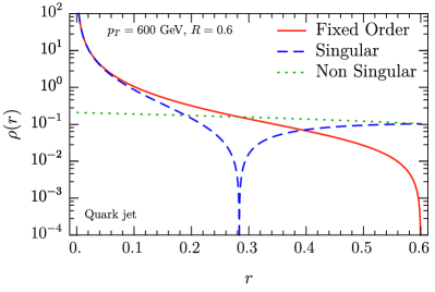
Refer to caption
Refer to caption

.

Figure 7: The differential jet shape at order αssubscript𝛼𝑠\alpha_{s} for quark jets (left) and gluon jets (right) at pT=600subscript𝑝𝑇600p_{T}=600 GeV and R=0.6𝑅0.6R=0.6. Shown are ρrRsubscript𝜌less-than-or-similar-to𝑟𝑅\rho_{r\lesssim R} (red solid), decomposed in its singular ρrRsubscript𝜌much-less-than𝑟𝑅\rho_{r\ll R} (blue dashed) and nonsingular (green dotted) contribution that correspond to the power corrections in eq. (20).

To determine the transition points xisubscript𝑥𝑖x_{i} in eq. (61), we assess the numerical size of the corrections to the factorization of ψrRsubscript𝜓much-less-than𝑟𝑅\psi_{r\ll R} at 𝒪(αs)𝒪subscript𝛼𝑠\mathcal{O}(\alpha_{s}), shown in fig. 7. The solid red curve shows the differential jet shape, the blue dashed curve shows its singular contribution obtained from the factorization in eq. (20), and the green dotted curve is the difference (often called the nonsingular), all at 𝒪(αs)𝒪subscript𝛼𝑠\mathcal{O}(\alpha_{s}). It is essential that the resummation of logarithms of r/R𝑟𝑅r/R is turned off before we enter the region where the singular is no longer a good approximation to the full jet shape, leading us to choose

x1=0.15,x2=(x1+x3)/2,x3=0.38.formulae-sequencesubscript𝑥10.15formulae-sequencesubscript𝑥2subscript𝑥1subscript𝑥32subscript𝑥30.38\displaystyle x_{1}=0.15\,,\qquad x_{2}=(x_{1}+x_{3})/2\,,\qquad x_{3}=0.38. (62)

Specifically, x1subscript𝑥1x_{1} corresponds roughly to the point where the nonsingular is 10% of the cross section, and x3subscript𝑥3x_{3} is chosen close to the point where the singular and nonsingular are equal in size. These points are somewhat arbitrarily chosen, and will be varied as part of the uncertainty estimate.

4.3 Scale variations and perturbative uncertainties

For our uncertainty estimate, we take the envelope of the following variations {enumerate*}

Vary all scales in eq. (4.1) simultaneously up and down by a factor of 2.

Vary μsubscript𝜇\mu_{\cal H} and μHsubscript𝜇𝐻\mu_{H} simultaneously up and down by a factor of 2.

Vary μCsubscript𝜇𝐶\mu_{C} and μSsubscript𝜇𝑆\mu_{S} simultaneously up and down by a factor of 2.

Vary νCsubscript𝜈𝐶\nu_{C} up and down by a factor of 2.

Vary νSsubscript𝜈𝑆\nu_{S} up and down by a factor of 2.

Vary the transition point x3subscript𝑥3x_{3} between 0.33 to 0.48. We can interpret the first as a fixed-order uncertainty, since it only changes the overall scales and not the ratios between them, which are the logarithms that are being resummed. The second and third variation probe the μ𝜇\mu resummation, since they vary the hierarchy between μHsubscript𝜇𝐻\mu_{H} and μC=μSsubscript𝜇𝐶subscript𝜇𝑆\mu_{C}=\mu_{S}, and similarly the fourth and fifth probe the rapidity resummation. While the evolution kernels are very similar for the variations in 2 and 3, the scales of different fixed-order ingredients are probed: The change in the evolution kernel is (partially) cancelled by a corresponding change in H𝐻H for variation 2 and by CStensor-product𝐶𝑆C\otimes S for variation 3, so they are not redundant. The same is true for variations 4 and 5. Variation 6 probes the uncertainty from our interpolation between the resummation and fixed-order region. We also explored the dependence on the transition point x1subscript𝑥1x_{1}, but it has a small effect and thus would not impact the total uncertainty.

4.4 First results for quark and gluon jets
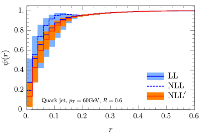
Refer to caption
Refer to caption

.
Refer to caption Refer to caption .

Figure 8: The integrated jet shape for quark jets (left) and gluon jets (right) for pT=subscript𝑝𝑇absentp_{T}= 60 GeV (top) and 500 GeV (bottom) and R=0.6𝑅0.6R=0.6. Shown are LL (blue solid curve and band), NLL (blue dashed curve) and NLL (orange solid curve and band), all matched to NLO. The bands indicate the perturbative uncertainties estimated using the procedure in sec. 4.3.
Refer to caption
Refer to caption

.
Refer to caption Refer to caption .

Figure 9: The integrated (left) and differential (right) jet shape for quark jets (blue) and gluon jets (green) at NLL with pT=500subscript𝑝𝑇500p_{T}=500 GeV and R=0.6𝑅0.6R=0.6. The top row shows the result with (solid) and without (dashed) rapidity resummation. The bottom row shows the result with (solid) and without (dashed) non-global logarithms.

In fig. 8 we show the integrated jet shape for quark and gluon jets with transverse momentum 60 and 500 GeV, comparing LL, NLL and NLL, all matched to NLO. We start by noting that our resummed calculations converge, i.e. the bands overlap and are smaller at NLL than at LL. As these plots show, the uncertainty bands are larger at small pTsubscript𝑝𝑇p_{T} and for gluon jets, which is not surprising since the perturbative corrections are simply larger in these cases due to the size of αssubscript𝛼𝑠\alpha_{s} and the color factor (CAsubscript𝐶𝐴C_{A} vs. CFsubscript𝐶𝐹C_{F}), respectively. At LL the bands are quite large, and they remain sizable at NLL, even though this exceeds the accuracy of previous jet shape calculations. We believe that this is due to our more conservative uncertainty estimate, described in sec. 4.3. Indeed, for gluon jets with pT=60subscript𝑝𝑇60p_{T}=60 GeV, the NLL central curve lies only just inside the LL uncertainty, warranting these large bands. For large r𝑟r all predictions overlap, since in each case we match to NLO. In this region there are no large logarithms of r/R𝑟𝑅r/R, so it is not surprising that the uncertainties are small. It is hard to gauge whether their size is reasonable, since we only have one perturbative order in this region (at LO ψ(r)𝜓𝑟\psi(r) is simply 1). Lastly we note that the NLL curve is not monotonic. That this unphysical behavior arises at NLL but not LL is due to the non-cusp anomalous dimension, whose contribution becomes equal and opposite in size to that of the cusp anomalous dimension. At NLL this is remedied by the inclusion of one-loop corrections to the ingredients in the factorization formula.

Fig. 9 illustrates the effect of the rapidity resummation and non-global logarithms on the jet shape for quark and gluon jets, by showing the integrated and differential jet shape with and without them. Both effects enter for the first time at NLL and were not taken into account in previous calculations. They are clearly important for rRmuch-less-than𝑟𝑅r\ll R, where their size is about half that of the NLL uncertainty band in fig. 8, but are of course irrelevant in the region where the resummation of logarithms of r/R𝑟𝑅r/R is turned off. The effect of the rapidity resummation is still significant in the transition region and is only turned off by the matching to fixed order, whereas the effect of NGLs is already small before the transition. The NGLs push the energy distribution in the jet out to larger values of r𝑟r, in agreement with the trend observed in e.g. ref. Dasgupta:2012hg for the jet mass distribution. This is clear from the integrated jet shape, and in the differential jet shape this arises through a decrease in the first bin (not as visible due to the logarithmic scale) and an increase in subsequent bins.

5 Nonperturbative effects

At the LHC, nonperturbative corrections to the jet shape can be large, particularly for smaller values of the jet pTsubscript𝑝𝑇p_{T}. These arise from the underlying event and hadronization effects. In this section we will explore simple models to account for these effects in our predictions. We will use Pythia 8.2 Sjostrand:2014zea to assess how reasonable these models are, by applying them to parton level predictions and comparing the result to hadron level predictions, including multi-parton interactions and initial-state radiation999This is not a nonperturbative contribution. However, we include it, because in our approach initial-state radiation is formally 𝒪(R2)𝒪superscript𝑅2\mathcal{O}(R^{2}) suppressed.. When we later apply this model to our predictions, we will use LHC data to fit the model parameter.

In the first model, we treat these effects by simply adding a uniform energy density to the jets. Explicitly

Model 1:ρ(r)2f1+frR2+11+fρ(r),Model 1:𝜌𝑟2𝑓1𝑓𝑟superscript𝑅211𝑓𝜌𝑟\displaystyle\text{Model 1:}\quad\rho(r)\to\frac{2f}{1+f}\frac{r}{R^{2}}+\frac{1}{1+f}\rho(r)\,, (63)

where ρ(r)𝜌𝑟\rho(r) is the differential jet shape and the fraction f𝑓f describes the size of the nonperturbative radiation compared to the perturbative contribution from our calculation. The dependence on r/R𝑟𝑅r/R is linear because it scales with the circumference of the circle of radius r𝑟r.

Refer to caption
Refer to caption

.
Refer to caption Refer to caption .

Figure 10: Jet shape in Pythia at Ecm=7subscript𝐸cm7E_{\rm cm}=7 TeV for anti-kTsubscript𝑘𝑇k_{T} jets with radius R=0.6𝑅0.6R=0.6, rapidity |η|<2.8𝜂2.8|\eta|<2.8 and transverse momentum pT=3040subscript𝑝𝑇3040p_{T}=30-40 GeV (left) and pT=6080subscript𝑝𝑇6080p_{T}=60-80 GeV (right). The top row shows results at parton level (blue dotted), including initial-state radiation (green dot-dashed), also multi-parton interactions (magenta dashed), and also hadronization (blue solid). The bottom row repeats the blue dotted and solid curves, where the effect of ISR, MPI and hadronization are either modeled using eq. (63) (green dot-dashed) or eq. (64) (orange dashed), and the parameter f𝑓f is fitted.

In the second model, the nonperturbative effects are again treated by adding energy. However, rather than considering a uniform distribution, we will assume this additional energy is completely localized, thus displacing the jet axis. The location (r,ϕ)superscript𝑟superscriptitalic-ϕ(r^{\prime},\phi^{\prime}) of this extra energy is then (uniformly) integrated over the jet. In terms of the differential jet shape ρ(r)𝜌𝑟\rho(r) this amounts to

Model 2:ρ(r)Model 2:𝜌𝑟absent\displaystyle\text{Model 2:}\quad\rho(r)\to 1π(1+f)2R20(1+f)Rdrr02πdϕ{f1+fδ(rr1+f)\displaystyle\frac{1}{\pi(1+f)^{2}R^{2}}\int_{0}^{(1+f)R}\!\mathrm{d}r^{\prime}\,r^{\prime}\!\int_{0}^{2\pi}\!\mathrm{d}\phi^{\prime}\bigg{\{}\frac{f}{1+f}\,\delta\Big{(}r-\frac{r^{\prime}}{1+f}\Big{)} (64)
+11+f0Rdr′′ρ(r′′)δ[r((r′′)2+2rr′′f1+fcosϕ+(r)2f2(1+f)2)1/2]}\displaystyle+\frac{1}{1\!+\!f}\,\int_{0}^{R}\!\mathrm{d}r^{\prime\prime}\,\rho^{\prime}(r^{\prime\prime})\,\delta\bigg{[}r\!-\!\bigg{(}(r^{\prime\prime})^{2}\!+\!\frac{2r^{\prime}r^{\prime\prime}f}{1\!+\!f}\cos\phi\!+\!\frac{(r^{\prime})^{2}f^{2}}{(1\!+\!f)^{2}}\bigg{)}^{1/2}\bigg{]}\bigg{\}}
=2f1+frR2+4rπf2(1+f)R2max{0,rfR}min{R,r+fR}dr′′ρ(r′′)absent2𝑓1𝑓𝑟superscript𝑅24𝑟𝜋superscript𝑓21𝑓superscript𝑅2superscriptsubscript0𝑟𝑓𝑅𝑅𝑟𝑓𝑅differential-dsuperscript𝑟′′𝜌superscript𝑟′′\displaystyle=\frac{2f}{1+f}\,\frac{r}{R^{2}}+\frac{4r}{\pi f^{2}(1+f)R^{2}}\int_{\max\{0,r-fR\}}^{\min\{R,r+fR\}}\!\mathrm{d}r^{\prime\prime}\,\rho(r^{\prime\prime})
|rr′′|min{1,r+r′′}drr2(r2+(r)2)(r′′)2(r2(r)2)2(r′′)4,superscriptsubscriptsubscript𝑟subscriptsuperscript𝑟′′1subscript𝑟subscriptsuperscript𝑟′′differential-dsubscriptsuperscript𝑟subscriptsuperscript𝑟2superscriptsubscript𝑟2superscriptsubscriptsuperscript𝑟2superscriptsubscriptsuperscript𝑟′′2superscriptsuperscriptsubscript𝑟2superscriptsubscriptsuperscript𝑟22superscriptsubscriptsuperscript𝑟′′4\displaystyle\quad\int_{|r_{*}-r^{\prime\prime}_{*}|}^{\min\{1,r_{*}+r^{\prime\prime}_{*}\}}\,\mathrm{d}r^{\prime}_{*}\,\frac{r^{\prime}_{*}}{\sqrt{2(r_{*}^{2}+(r^{\prime}_{*})^{2})(r^{\prime\prime}_{*})^{2}-(r_{*}^{2}-(r^{\prime}_{*})^{2})^{2}-(r^{\prime\prime}_{*})^{4}}}\,,

The first term in the curly brackets (on the first line) corresponds to the contribution to the jet shape from the extra energy. Upon integration this results in the first term on the third line, in agreement with eq. (63). However, the jet shape also gets smeared by the displacement of the jet axis. Specifically, the r′′superscript𝑟′′r^{\prime\prime} integral in the second term integrates over the jet shape, taking into account the displacement from the extra energy at (r,ϕ)superscript𝑟superscriptitalic-ϕ(r^{\prime},\phi^{\prime}) through the delta function. In the final expression we eliminated the ϕsuperscriptitalic-ϕ\phi^{\prime} integral using the delta function, and introduced

r=rfR,r=r(1+f)R,r′′=r′′fRformulae-sequencesubscript𝑟𝑟𝑓𝑅formulae-sequencesubscriptsuperscript𝑟superscript𝑟1𝑓𝑅subscriptsuperscript𝑟′′superscript𝑟′′𝑓𝑅\displaystyle r_{*}=\frac{r}{fR}\,,\qquad r^{\prime}_{*}=\frac{r^{\prime}}{(1+f)R}\,,\qquad r^{\prime\prime}_{*}=\frac{r^{\prime\prime}}{fR} (65)

to remove any explicit dependence on f𝑓f and R𝑅R in the rsuperscript𝑟r^{\prime} integral. Thus we can determine this integral numerically once and for all, to obtain the kernel against which we integrate the jet shape in the remaining r′′superscript𝑟′′r^{\prime\prime} integral.

In fig. 10 we show the partonic and hadronic jet shape obtained from Pythia, and investigate to what extent multiparton interactions, initial-state radiation and hadronization effects can be described by one of the models above. The top row shows the contribution of each of these effects, the bottom row shows a fit (of the coefficient f𝑓f) to these effects using one of the models proposed here. We find better agreement using model 2, suggesting that these nonperturbative effects are at least fairly localized in the jet. We therefore use model 2 when we compare our results to LHC data in the next section.

6 Results for the LHC
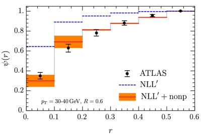
Refer to caption
Refer to caption

.
Refer to caption Refer to caption .

Figure 11: Comparison of our theoretical calculation at NLL accuracy for the inclusive jet shape ψ(r)𝜓𝑟\psi(r) to the data from ATLAS Aad:2011kq . The inclusive anti-kT jet sample is reconstructed for a jet radius of R=0.6𝑅0.6R=0.6 and |η|<2.8𝜂2.8|\eta|<2.8 measured at Ecm=7subscript𝐸cm7E_{\rm cm}=7 TeV. Four representative jet pTsubscript𝑝𝑇p_{T} intervals in the range 306003060030-600 GeV are shown, as indicated in the panels. Our purely perturbative calculation is shown (dashed blue), along with the results that include the nonperturbative effects through a model (orange) and perturbative uncertainty band.

In this section, we present comparisons of our theoretical results to data from ATLAS and CMS. We start with the ATLAS data for the integrated and differential jet shape of ref. Aad:2011kq . Although the central values of the differential and integrated jet shape are directly related, their uncertainties are not because of correlations, which is why we show results for both. The inclusive jet sample ppjet+X𝑝𝑝jet𝑋pp\to{\rm jet}+X was obtained using the anti-kT algorithm with R=0.6𝑅0.6R=0.6. The jet rapidity was restricted to |η|<2.8𝜂2.8|\eta|<2.8, and different intervals for its transverse momentum pTsubscript𝑝𝑇p_{T} in the range of 306003060030-600 GeV were considered. In fig. 11, we show a comparison of our numerical results to the ATLAS data for the integrated jet shape ψ(r)𝜓𝑟\psi(r) for four representative pTsubscript𝑝𝑇p_{T} intervals, as indicated in the different panels. For all phenomenological results presented in this section, we use the CT14 NLO PDF set of ref. Dulat:2015mca . We show both the purely perturbative calculation (dashed blue curve) as well as the results after including the nonperturbative “model 2” (orange curve and band), described in section 5. The QCD scale uncertainty is shown only for the final result including the nonperturbative contribution, following the procedure discussed in section 4.3. The parameter f𝑓f of the nonperturbative model is determined from fitting our central curve to the central value of the data. Its value is tabulated in table 3 for each pTsubscript𝑝𝑇p_{T} interval. At smaller values of the jet transverse momentum, the purely perturbative result and the data disagree significantly, where the perturbative calculation predicts that there is more radiation close to the center of the jet and less near the jet boundary. Nevertheless, we find that the data is well described after including a nonperturbative correction. As is clear from the plots and the table, at higher values of pTsubscript𝑝𝑇p_{T} the nonperturbative correction becomes smaller. Indeed, for the highest transverse momentum interval 500600500600500-600 GeV we already find a good agreement between the data and our purely perturbative calculation obtained from the QCD factorization theorem. Because the nonperturbative model parametrizes the effect of nonperturbative physics relative to the perturbative prediction for the jet, rather than through some absolute energy scale, it is not surprising that approximately f1/pTsimilar-to𝑓1subscript𝑝𝑇f\sim 1/p_{T}.

Refer to caption
Refer to caption

.
Refer to caption Refer to caption .

Figure 12: Comparison of our numerical results for the differential jet shape ρ(r)𝜌𝑟\rho(r) and the ATLAS data of Aad:2011kq , for the same kinematics as in fig. 11.
ATLAS Aad:2011kq pTsubscript𝑝𝑇p_{T} [GeV] 30-40 60-80 110-160 500-600
Ecm=7subscript𝐸cm7E_{\rm cm}=7 TeV f𝑓f 0.23 0.16 0.11 0.062
CMS Chatrchyan:2012mec pTsubscript𝑝𝑇p_{T} [GeV] 30-40 500-600 600-1000
Ecm=7subscript𝐸cm7E_{\rm cm}=7 TeV f𝑓f 0.28 0.068 0.054
CMS Chatrchyan:2013kwa pTsubscript𝑝𝑇p_{T} [GeV] >100absent100>100
Ecm=2.76subscript𝐸cm2.76E_{\rm cm}=2.76 TeV f𝑓f 0.050
Table 3: Fitted values for the parameter f𝑓f of the nonperturbative “model 2”, for the jet transverse momentum intervals of the ATLAS Aad:2011kq and CMS Chatrchyan:2012mec ; Chatrchyan:2013kwa data that we show here. Note that the jet radius R𝑅R and the rapidity intervals η𝜂\eta differ between the different data sets.

In fig. 12, we show our numerical results for the differential jet shape ρ(r)𝜌𝑟\rho(r) in comparison to the corresponding ATLAS data for the same jet kinematics. We use the same f𝑓f values for the nonperturbative model as for the integrated jet shape. Again we observe that a large nonperturbative correction is needed to describe the differential jet shape data for jets with low transverse momentum. This is particularly pronounced close to the jet boundary, where no resummation of r/R𝑟𝑅r/R is required, and the fixed-order expressions in eq. (2.2) clearly undershoot the data. (This was not so visible for the integrated jet shape, since everything is close to one.) For the higher transverse momentum bins, the agreement between the data and the purely perturbative results is improved and only a smaller nonperturbative correction is needed. However, close to the jet boundary, the effect of the nonperturbative correction remains substantial, even for the highest pTsubscript𝑝𝑇p_{T} interval. We note that for pT=3040subscript𝑝𝑇3040p_{T}=30-40 GeV, the nonperturbative model causes the second bin to be higher than the first. This feature is already visible in fig. 10, both for our model 2 and the curve for Pythia at hadron level, since the integrated jet shape is not the steepest at r=0𝑟0r=0.

Refer to caption
Refer to caption

.
Refer to caption .

Figure 13: Comparison of our numerical results for the differential jet shape ρ(r)𝜌𝑟\rho(r) to the CMS data of ref. Chatrchyan:2012mec . The jets are obtained using anti-kT with R=0.7𝑅0.7R=0.7 and, |η|<0.5𝜂0.5|\eta|<0.5 at Ecm=7subscript𝐸cm7E_{\rm cm}=7 TeV. We show the result for three intervals of the jet transverse momentum in the range of pT=301000subscript𝑝𝑇301000p_{T}=30-1000 GeV, as labeled in the different panels.

Next, we consider the CMS data set of ref. Chatrchyan:2012mec for the differential jet shape ρ(r)𝜌𝑟\rho(r), which was also measured at a center-of-mass energy of Ecm=7subscript𝐸cm7E_{\rm cm}=7 TeV. The kinematics of the reconstructed inclusive jet sample is similar to the setup from ATLAS, but now using anti-kT with R=0.7𝑅0.7R=0.7, |η|<0.5𝜂0.5|\eta|<0.5 and dividing the jet transverse momentum pTsubscript𝑝𝑇p_{T} into several intervals in the range of 30100030100030-1000 GeV. In fig. 13 we show the comparison of our numerical results with and without the nonperturbative contribution. We again fit the nonperturbative parameter f𝑓f of “model 2”, listing their values in table 3. These values are consistent with those obtained for ATLAS, in the cases for which we have a corresponding pTsubscript𝑝𝑇p_{T} interval. (They do not need to be exactly the same, given the difference in jet radius and rapidity interval.) We note again that even for the highest jet transverse momentum interval pT=6001000subscript𝑝𝑇6001000p_{T}=600-1000 GeV a significant nonperturbative correction is needed in order to describe the energy distribution close to the edge of the jet, rRless-than-or-similar-to𝑟𝑅r\lesssim R, as we also observed for the ATLAS data.

Finally, we compare to the differential jet shape measurement of CMS in ref. Chatrchyan:2013kwa . This data set was taken at s=2.76𝑠2.76\sqrt{s}=2.76 TeV as a baseline measurement for a heavy-ion analysis. The jets were reconstructed with pT>100subscript𝑝𝑇100p_{T}>100 GeV and 0.3<|η|<20.3𝜂20.3<|\eta|<2 using the anti-kT algorithm with R=0.3𝑅0.3R=0.3. Analogous to the two data sets discussed above, the jet shape data is separated into six bins with a distance in r𝑟r of 0.05. An additional cut of pTi>1subscript𝑝𝑇𝑖1p_{Ti}>1 GeV was imposed on the transverse momentum of each particle in the jet, and only charged particles are used to determine the jet shape even though full jets are reconstructed. Furthermore, the jet pTsubscript𝑝𝑇p_{T} was smeared to account for the difference of the jet energy resolution between proton-proton and heavy-ion collisions. This should be kept in mind when comparing to our calculation, since we do not include these effects. Nevertheless, we find good agreement as shown in fig. 14. The edge of the jet is still dominated by nonperturbative physics for R=0.3𝑅0.3R=0.3. However, the data is closer to the purely perturbative result compared to the jet shape for a similar pTsubscript𝑝𝑇p_{T} interval in fig. 12 for R=0.6𝑅0.6R=0.6 jets. Indeed, the fitted value of the nonperturbative parameter f𝑓f, see table 3, is about half of that for the pTsubscript𝑝𝑇p_{T} interval 110-160 GeV in the ATLAS data. This is not surprising, given the lower center-of-mass energy and the smaller jet radius. In general, we conclude that our numerical results agree well with the data, once the nonperturbative correction is taken into account.
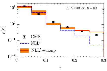
Refer to caption
Figure 14: Comparison of the differential jet shape ρ(r)𝜌𝑟\rho(r) and the CMS data of ref. Chatrchyan:2013kwa . The jets are obtained using anti-kT with R=0.3𝑅0.3R=0.3, pT>100subscript𝑝𝑇100p_{T}>100 GeV, 0.3<|η|<20.3𝜂20.3<|\eta|<2 at Ecm=2.76subscript𝐸cm2.76E_{\rm cm}=2.76 TeV.

7 Conclusions

In this paper we calculate the jet shape at next-to-leading logarithmic accuracy (NLL). Specifically, we account for the single logarithms of the jet radius R𝑅R and the double logarithms of r/R𝑟𝑅r/R at next-to-leading logarithmic order, and match to next-to-leading order. To achieve this accuracy, the recoil of soft radiation on the jet axis must be included when rRmuch-less-than𝑟𝑅r\ll R. This involves the one-loop calculation of a recoil-sensitive collinear function and rapidity logarithms, that we resum using the rapidity renormalization group, as well as non-global logarithms from in vs. out-of-jet soft radiation. Our calculation constitutes the first extension of this classic jet substructure observable beyond leading logarithmic accuracy.

The inclusion of higher-order corrections significantly reduces the uncertainty of the perturbative predictions. However, we also find that the effect of nonperturbative contributions are substantial at the LHC, in particular for low jet transverse momenta and close to the edge of the jet. To enable a comparison to the available data from ATLAS and CMS, we explored two one-parameter models, choosing the model that best captures these effects in Pythia. Including this, we find good agreement between our predictions and LHC data. One interesting future direction is to obtain predictions that can be compared to LEP and HERA data, where these nonperturbative effects should be substantially smaller. On the other hand, for the LHC it is natural to consider grooming, to reduce the contamination from these effects, which will be the topic of a forthcoming publication CKLRW .

Acknowledgements.
We thank Y.-J. Lee, B. Nachman, D. Neill, N. Sato and F. Yuan for discussions and K. Lee for feedback on the manuscript. This work is supported by the U.S. Department of Energy under Contract No. DE-AC02-05CH11231, the LDRD Program of Lawrence Berkeley National Laboratory, by the ERC grant ERC-STG-2015-677323 and the D-ITP consortium, a program of the Netherlands Organization for Scientific Research (NWO) that is funded by the Dutch Ministry of Education, Culture and Science (OCW).

Appendix A Jet function for the jet shape when 𝐫𝐑less-than-or-similar-to𝐫𝐑\mathbf{r\lesssim R}

The jet function (or central subjet function) in eq. (2.1) for the anti-kTsubscript𝑘𝑇k_{T} algorithm is up to one-loop order given by Kang:2017mda

𝒢qjet(z,zr,pTR,r/R,μ)superscriptsubscript𝒢𝑞jet𝑧subscript𝑧𝑟subscript𝑝𝑇𝑅𝑟𝑅𝜇\displaystyle{\mathcal{G}}_{q}^{\mathrm{jet}}(z,z_{r},p_{T}R,r/R,\mu)
=δ(1z)δ(1zr)+αs2π{δ(1zr)LR[Pqq(z)+Pgq(z)]δ(1zr)[2CF(1+z2)(ln(1z)1z)+\displaystyle=\delta(1\!-\!z)\delta(1\!-\!z_{r})+\frac{\alpha_{s}}{2\pi}\bigg{\{}\delta(1\!-\!z_{r})L_{R}\left[P_{qq}(z)+P_{gq}(z)\right]-\delta(1\!-\!z_{r})\bigg{[}2C_{F}(1\!+\!z^{2})\Big{(}\frac{\ln(1\!-\!z)}{1-z}\Big{)}_{+}
+2Pgq(z)ln(1z)+CF]+δ(1z)θ(zr>12)[Pqq(zr)+Pgq(zr)](Lr/R+2lnzr)\displaystyle\quad+2P_{gq}(z)\ln(1-z)+C_{F}\bigg{]}+\delta(1-z)\theta\Big{(}z_{r}>\frac{1}{2}\Big{)}[P_{qq}(z_{r})+P_{gq}(z_{r})](L_{r/R}+2\ln z_{r})
+θ(r<R/2)[δ(1z)δ(1zr)CF(72+3ln2π23)\displaystyle\quad+\theta(r<R/2)\bigg{[}\delta(1-z)\delta(1-z_{r})C_{F}\bigg{(}\frac{7}{2}+3\ln 2-\frac{\pi^{2}}{3}\bigg{)}
δ(1z)θ(12<zr<1rR)[Pqq(zr)+Pgq(zr)](Lr/R+2ln(1zr))]\displaystyle\qquad-\delta(1-z)\theta\Big{(}\frac{1}{2}<z_{r}<1-\frac{r}{R}\Big{)}[P_{qq}(z_{r})+P_{gq}(z_{r})]\big{(}L_{r/R}+2\ln(1-z_{r})\big{)}\bigg{]}
+θ(r>R/2)[δ(1z)δ(1zr)CF(12Lr/R2+32Lr/R2Lr/Rln(1rR)+4Li2(1rR)\displaystyle\quad+\theta(r>R/2)\bigg{[}\delta(1\!-\!z)\delta(1\!-\!z_{r})\,C_{F}\bigg{(}-\frac{1}{2}L_{r/R}^{2}+\frac{3}{2}L_{r/R}-2L_{r/R}\ln\Big{(}1\!-\!\frac{r}{R}\Big{)}+4\text{Li}_{2}\Big{(}1\!-\!\frac{r}{R}\Big{)}
+122π23+6rR)δ(1z)θ(12<zr<rR)[Pqq(zr)+Pgq(zr)](Lr/R+2lnzr)]},\displaystyle\qquad+\frac{1}{2}-\frac{2\pi^{2}}{3}+6\frac{r}{R}\bigg{)}-\delta(1-z)\theta\Big{(}\frac{1}{2}<z_{r}<\frac{r}{R}\Big{)}[P_{qq}(z_{r})+P_{gq}(z_{r})]\big{(}L_{r/R}+2\ln z_{r}\big{)}\bigg{]}\bigg{\}}\,,
𝒢gjet(z,zr,pTR,r/R,μ)superscriptsubscript𝒢𝑔jet𝑧subscript𝑧𝑟subscript𝑝𝑇𝑅𝑟𝑅𝜇\displaystyle{\mathcal{G}}_{g}^{\mathrm{jet}}(z,z_{r},p_{T}R,r/R,\mu)
=δ(1z)δ(1zr)+αs2π{δ(1zr)LR[Pgg(z)+2nfPqg(z)]\displaystyle=\delta(1-z)\delta(1-z_{r})+\frac{\alpha_{s}}{2\pi}\bigg{\{}\delta(1-z_{r})L_{R}\big{[}P_{gg}(z)+2n_{f}P_{qg}(z)\big{]}
+δ(1z)θ(zr>12)[Pgg(zr)+2nfPqg(zr)](Lr/R+2lnzr)𝛿1𝑧𝜃subscript𝑧𝑟12delimited-[]subscript𝑃𝑔𝑔subscript𝑧𝑟2subscript𝑛𝑓subscript𝑃𝑞𝑔subscript𝑧𝑟subscript𝐿𝑟𝑅2subscript𝑧𝑟\displaystyle\quad+\delta(1-z)\theta\Big{(}z_{r}>\frac{1}{2}\Big{)}[P_{gg}(z_{r})+2n_{f}P_{qg}(z_{r})](L_{r/R}+2\ln z_{r})
δ(1zr)[4CA(1z+z2)2z(ln(1z)1z)++4nf(Pqg(z)ln(1z)+TFz(1z))]𝛿1subscript𝑧𝑟delimited-[]4subscript𝐶𝐴superscript1𝑧superscript𝑧22𝑧subscript1𝑧1𝑧4subscript𝑛𝑓subscript𝑃𝑞𝑔𝑧1𝑧subscript𝑇𝐹𝑧1𝑧\displaystyle\quad-\delta(1-z_{r})\bigg{[}4C_{A}\frac{(1-z+z^{2})^{2}}{z}\Big{(}\frac{\ln(1-z)}{1-z}\Big{)}_{+}+4n_{f}\big{(}P_{qg}(z)\ln(1-z)+T_{F}z(1-z)\big{)}\bigg{]}
+θ(r<R/2)[δ(1z)δ(1zr)(CA(13736+113ln2π23)TFnf(2318+43ln2))\displaystyle\quad+\theta(r<R/2)\bigg{[}\delta(1-z)\delta(1-z_{r})\bigg{(}C_{A}\bigg{(}\frac{137}{36}+\frac{11}{3}\ln 2-\frac{\pi^{2}}{3}\bigg{)}-T_{F}n_{f}\bigg{(}\frac{23}{18}+\frac{4}{3}\ln 2\bigg{)}\bigg{)}
δ(1z)θ(12<zr<1rR)[Pgg(z)+2nfPqg(z)](Lr/R+2ln(1zr))]\displaystyle\qquad-\delta(1-z)\theta\Big{(}\frac{1}{2}<z_{r}<1-\frac{r}{R}\Big{)}[P_{gg}(z)+2n_{f}P_{qg}(z)]\big{(}L_{r/R}+2\ln(1-z_{r})\big{)}\bigg{]}
+θ(r>R/2)[δ(1z)δ(1zr)[CA2Lr/R2+β02Lr/R2CALr/Rln(1rR)\displaystyle\quad+\theta(r>R/2)\bigg{[}\delta(1-z)\delta(1-z_{r})\bigg{[}-\frac{C_{A}}{2}L_{r/R}^{2}+\frac{\beta_{0}}{2}L_{r/R}-2C_{A}L_{r/R}\ln\Big{(}1-\frac{r}{R}\Big{)}
+4CALi2(1rR)CA2π23+CA(8rRr2R2+4r39R3)+TFnf(134rR+2r2R28r39R3))\displaystyle\qquad+4C_{A}\text{Li}_{2}\Big{(}1\!-\!\frac{r}{R}\Big{)}-C_{A}\frac{2\pi^{2}}{3}+C_{A}\Big{(}\frac{8r}{R}-\frac{r^{2}}{R^{2}}+\frac{4r^{3}}{9R^{3}}\Big{)}+T_{F}n_{f}\Big{(}\frac{1}{3}-\frac{4r}{R}+\frac{2r^{2}}{R^{2}}-\frac{8r^{3}}{9R^{3}}\Big{)}\!\bigg{)}
δ(1z)θ(12<zr<rR)[Pgg(z)+2nfPqg(z)](Lr/R+2lnzr)]}.\displaystyle\qquad-\delta(1-z)\theta\left(\frac{1}{2}<z_{r}<\frac{r}{R}\right)[P_{gg}(z)+2n_{f}P_{qg}(z)]\left(L_{r/R}+2\ln z_{r}\right)\bigg{]}\bigg{\}}\,. (66)

The splitting functions Pijsubscript𝑃𝑖𝑗P_{ij} are given in eq. (2.1), and we use the following short-hand notation

LR=ln(μ2pT2R2),Lr=ln(μ2pT2r2),Lr/RLrLR=ln(R2r2).formulae-sequencesubscript𝐿𝑅superscript𝜇2superscriptsubscript𝑝𝑇2superscript𝑅2formulae-sequencesubscript𝐿𝑟superscript𝜇2superscriptsubscript𝑝𝑇2superscript𝑟2subscript𝐿𝑟𝑅subscript𝐿𝑟subscript𝐿𝑅superscript𝑅2superscript𝑟2\displaystyle L_{R}=\ln\Big{(}\frac{\mu^{2}}{p_{T}^{2}R^{2}}\Big{)}\,,\qquad L_{r}=\ln\Big{(}\frac{\mu^{2}}{p_{T}^{2}r^{2}}\Big{)}\,,\qquad L_{r/R}\equiv L_{r}-L_{R}=\ln\Big{(}\frac{R^{2}}{r^{2}}\Big{)}\,. (67)

Appendix B Anomalous dimensions

The one-loop anomalous dimensions directly follow from the expressions in secs. 2.3, 2.4 and 3,

γqqH(z,pTR,μ)subscriptsuperscript𝛾𝐻𝑞𝑞𝑧subscript𝑝𝑇𝑅𝜇\displaystyle\gamma^{H}_{qq}(z,p_{T}R,\mu) =αsπ[CF(LR32)δ(1z)+Pqq(z)],absentsubscript𝛼𝑠𝜋delimited-[]subscript𝐶𝐹subscript𝐿𝑅32𝛿1𝑧subscript𝑃𝑞𝑞𝑧\displaystyle=\frac{\alpha_{s}}{\pi}\bigg{[}C_{F}\Big{(}-L_{R}-\frac{3}{2}\Big{)}\,\delta(1-z)+P_{qq}(z)\bigg{]},
γqgH(z,pTR,μ)subscriptsuperscript𝛾𝐻𝑞𝑔𝑧subscript𝑝𝑇𝑅𝜇\displaystyle\gamma^{H}_{qg}(z,p_{T}R,\mu) =αsπPgq(z),absentsubscript𝛼𝑠𝜋subscript𝑃𝑔𝑞𝑧\displaystyle=\frac{\alpha_{s}}{\pi}\,P_{gq}(z),
γggH(z,pTR,μ)subscriptsuperscript𝛾𝐻𝑔𝑔𝑧subscript𝑝𝑇𝑅𝜇\displaystyle\gamma^{H}_{gg}(z,p_{T}R,\mu) =αsπ[(CALR12β0)δ(1z)+Pgg(z)],absentsubscript𝛼𝑠𝜋delimited-[]subscript𝐶𝐴subscript𝐿𝑅12subscript𝛽0𝛿1𝑧subscript𝑃𝑔𝑔𝑧\displaystyle=\frac{\alpha_{s}}{\pi}\bigg{[}\Big{(}-C_{A}L_{R}-\frac{1}{2}\beta_{0}\Big{)}\,\delta(1-z)+P_{gg}(z)\bigg{]},
γgqH(z,pTR,μ)subscriptsuperscript𝛾𝐻𝑔𝑞𝑧subscript𝑝𝑇𝑅𝜇\displaystyle\gamma^{H}_{gq}(z,p_{T}R,\mu) =αsπPqg(z),absentsubscript𝛼𝑠𝜋subscript𝑃𝑞𝑔𝑧\displaystyle=\frac{\alpha_{s}}{\pi}\,P_{qg}(z),
γqC(μ,ν/pT)subscriptsuperscript𝛾𝐶𝑞𝜇𝜈subscript𝑝𝑇\displaystyle\gamma^{C}_{q}(\mu,\nu/p_{T}) =αsCFπ(2lnν2pT+32),absentsubscript𝛼𝑠subscript𝐶𝐹𝜋2𝜈2subscript𝑝𝑇32\displaystyle=\frac{\alpha_{s}C_{F}}{\pi}\,\Big{(}2\ln\frac{\nu}{2p_{T}}+\frac{3}{2}\Big{)}\,,
γgC(μ,ν/pT)subscriptsuperscript𝛾𝐶𝑔𝜇𝜈subscript𝑝𝑇\displaystyle\gamma^{C}_{g}(\mu,\nu/p_{T}) =αsπ(2CAlnν2pT+12β0),absentsubscript𝛼𝑠𝜋2subscript𝐶𝐴𝜈2subscript𝑝𝑇12subscript𝛽0\displaystyle=\frac{\alpha_{s}}{\pi}\,\Big{(}2C_{A}\ln\frac{\nu}{2p_{T}}+\frac{1}{2}\beta_{0}\Big{)}\,,
γqS(μ,νR)subscriptsuperscript𝛾𝑆𝑞𝜇𝜈𝑅\displaystyle\gamma^{S}_{q}(\mu,\nu R) =αsCFπln4μ2ν2R2,absentsubscript𝛼𝑠subscript𝐶𝐹𝜋4superscript𝜇2superscript𝜈2superscript𝑅2\displaystyle=\frac{\alpha_{s}C_{F}}{\pi}\,\ln\frac{4\mu^{2}}{\nu^{2}R^{2}}\,,
γgS(μ,νR)subscriptsuperscript𝛾𝑆𝑔𝜇𝜈𝑅\displaystyle\gamma^{S}_{g}(\mu,\nu R) =αsCAπln4μ2ν2R2,absentsubscript𝛼𝑠subscript𝐶𝐴𝜋4superscript𝜇2superscript𝜈2superscript𝑅2\displaystyle=\frac{\alpha_{s}C_{A}}{\pi}\,\ln\frac{4\mu^{2}}{\nu^{2}R^{2}}\,,
γqν(k,μ)subscriptsuperscript𝛾𝜈𝑞subscript𝑘perpendicular-to𝜇\displaystyle\gamma^{\nu}_{q}(k_{\perp},\mu) =4αsCF1μ21(k2/μ2)+,absent4subscript𝛼𝑠subscript𝐶𝐹1superscript𝜇2subscript1superscriptsubscript𝑘perpendicular-to2superscript𝜇2\displaystyle=4\alpha_{s}C_{F}\,\frac{1}{\mu^{2}}\,\frac{1}{(k_{\perp}^{2}/\mu^{2})}_{+}\,,
γgν(k,μ)subscriptsuperscript𝛾𝜈𝑔subscript𝑘perpendicular-to𝜇\displaystyle\gamma^{\nu}_{g}(k_{\perp},\mu) =4αsCA1μ21(k2/μ2)+.absent4subscript𝛼𝑠subscript𝐶𝐴1superscript𝜇2subscript1superscriptsubscript𝑘perpendicular-to2superscript𝜇2\displaystyle=4\alpha_{s}C_{A}\,\frac{1}{\mu^{2}}\,\frac{1}{(k_{\perp}^{2}/\mu^{2})}_{+}\,. (68)

Here LRsubscript𝐿𝑅L_{R} is defined in eq. (67) and the splitting functions are given in eq. (2.1). To achieve NLL accuracy, we include the two-loop cusp anomalous dimensions for the lnμ𝜇\ln\mu and lnν𝜈\ln\nu terms in the anomalous dimensions. This amounts to multiplying these terms by

1+αs4π[(679π23)CA209TFnf].1subscript𝛼𝑠4𝜋delimited-[]679superscript𝜋23subscript𝐶𝐴209subscript𝑇𝐹subscript𝑛𝑓\displaystyle 1+\frac{\alpha_{s}}{4\pi}\Bigl{[}\Bigl{(}\frac{67}{9}-\frac{\pi^{2}}{3}\Bigr{)}\,C_{A}-\frac{20}{9}\,T_{F}\,n_{f}\Bigr{]}\,. (69)

Appendix C Rapidity anomalous dimension of the one-loop collinear function

We will now check that our expression for the collinear function satisfies the rapidity evolution equation in eq. (2.1), which expanded up to one-loop order reads

ddlnνCi(1)(zr,pTr,k,μ,ν)dd𝜈superscriptsubscript𝐶𝑖1subscript𝑧𝑟subscript𝑝𝑇𝑟subscript𝑘perpendicular-to𝜇𝜈\displaystyle\frac{\mathrm{d}}{\mathrm{d}\ln\nu}\,C_{i}^{(1)}(z_{r},p_{T}r,k_{\perp},\mu,\nu) =d2k(2π)2γiν(1)(kk,μ)Ci(0)(zr,pTr,k,μ,ν).absentsuperscriptd2superscriptsubscript𝑘perpendicular-tosuperscript2𝜋2subscriptsuperscript𝛾𝜈1𝑖subscript𝑘perpendicular-tosuperscriptsubscript𝑘perpendicular-to𝜇superscriptsubscript𝐶𝑖0subscript𝑧𝑟subscript𝑝𝑇𝑟superscriptsubscript𝑘perpendicular-to𝜇𝜈\displaystyle=-\int\!\frac{\mathrm{d}^{2}k_{\perp}^{\prime}}{(2\pi)^{2}}\,\gamma^{\nu(1)}_{i}(k_{\perp}-k_{\perp}^{\prime},\mu)\,C_{i}^{(0)}(z_{r},p_{T}r,k_{\perp}^{\prime},\mu,\nu)\,. (70)

Note that γiν(1)(k)superscriptsubscript𝛾𝑖𝜈1subscript𝑘perpendicular-to\gamma_{i}^{\nu(1)}(k_{\perp}) was already obtained from the soft function, so this provides a cross check. From eq. (52) we find that the left-hand side of eq. (70) is given by

dCi,θ<r(1)dlnνdsubscriptsuperscript𝐶1𝑖𝜃𝑟d𝜈\displaystyle\frac{\mathrm{d}C^{(1)}_{i,\theta<r}}{\mathrm{d}\ln\nu} =Θ(k<pTr)δ(1zr)αsCi2π202πdϕL1absentΘsubscript𝑘perpendicular-tosubscript𝑝𝑇𝑟𝛿1subscript𝑧𝑟subscript𝛼𝑠subscript𝐶𝑖2superscript𝜋2superscriptsubscript02𝜋differential-ditalic-ϕsubscript𝐿1\displaystyle=\Theta(k_{\perp}<p_{T}r)\,\delta(1-z_{r})\,\frac{\alpha_{s}C_{i}}{2\pi^{2}}\int_{0}^{2\pi}\mathrm{d}\phi\,L_{1}
+Θ(k>pTr)δ(1zr)αsCiπ2ϕmaxϕmaxdϕln(β2minβ2max),Θsubscript𝑘perpendicular-tosubscript𝑝𝑇𝑟𝛿1subscript𝑧𝑟subscript𝛼𝑠subscript𝐶𝑖superscript𝜋2superscriptsubscriptsubscriptitalic-ϕmaxsubscriptitalic-ϕmaxdifferential-ditalic-ϕsuperscriptsubscript𝛽2minsuperscriptsubscript𝛽2max\displaystyle\quad+\Theta(k_{\perp}>p_{T}r)\,\,\delta(1-z_{r})\,\frac{\alpha_{s}C_{i}}{\pi^{2}}\int_{-\phi_{\rm max}}^{\phi_{\rm max}}\mathrm{d}\phi\,\ln\Bigl{(}\frac{\beta_{2}^{\text{min}}}{\beta_{2}^{\text{max}}}\Bigr{)}, (71)

where the color factor is given by Cq=CFsubscript𝐶𝑞subscript𝐶𝐹C_{q}=C_{F} for quarks and Cg=CAsubscript𝐶𝑔subscript𝐶𝐴C_{g}=C_{A} for gluons.

Refer to caption
Refer to caption

.

Figure 15: The geometry of |kk|<pTrsubscript𝑘perpendicular-tosubscriptsuperscript𝑘perpendicular-tosubscript𝑝𝑇𝑟|k_{\perp}-k^{\prime}_{\perp}|<p_{T}r for |k|<pTrsubscript𝑘perpendicular-tosubscript𝑝𝑇𝑟|k_{\perp}|<p_{T}r (left) and |k|>pTrsubscript𝑘perpendicular-tosubscript𝑝𝑇𝑟|k_{\perp}|>p_{T}r (right).

Since the terms in eq. (C) correspond to θ<r𝜃𝑟\theta<r and θ>r𝜃𝑟\theta>r, respectively, it is natural to split up the calculation of the right-hand side of eq. (70) in the same pieces. For θ<r𝜃𝑟\theta<r this requires computing,

Θ(k<pTr)d2k(2π)21μ21(k2/μ2)+Θ(|kk|<pTr)Θsubscript𝑘perpendicular-tosubscript𝑝𝑇𝑟superscriptd2subscriptsuperscript𝑘perpendicular-tosuperscript2𝜋21superscript𝜇2subscript1superscriptsubscript𝑘perpendicular-to2superscript𝜇2Θsubscript𝑘perpendicular-tosubscriptsuperscript𝑘perpendicular-tosubscript𝑝𝑇𝑟\displaystyle\Theta(k_{\perp}<p_{T}r)\int\frac{\mathrm{d}^{2}k^{\prime}_{\perp}}{(2\pi)^{2}}\frac{1}{\mu^{2}}\frac{1}{(k_{\perp}^{\prime 2}/\mu^{2})}_{+}\Theta\bigl{(}|k_{\perp}-k^{\prime}_{\perp}|<p_{T}r\bigr{)}
=Θ(k<pTr)02πdϕ0(pTβ1maxμ)2d(k2/μ2)8π21(k2/μ2)+absentΘsubscript𝑘perpendicular-tosubscript𝑝𝑇𝑟superscriptsubscript02𝜋differential-ditalic-ϕsuperscriptsubscript0superscriptsubscript𝑝𝑇superscriptsubscript𝛽1max𝜇2dsubscriptsuperscript𝑘2perpendicular-tosuperscript𝜇28superscript𝜋2subscript1superscriptsubscript𝑘perpendicular-to2superscript𝜇2\displaystyle\quad=\Theta(k_{\perp}<p_{T}r)\int_{0}^{2\pi}\mathrm{d}\phi\int_{0}^{\big{(}\frac{p_{T}\beta_{1}^{\text{max}}}{\mu}\big{)}^{2}}\frac{\mathrm{d}(k^{\prime 2}_{\perp}/\mu^{2})}{8\pi^{2}}\frac{1}{(k_{\perp}^{\prime 2}/\mu^{2})}_{+}
=Θ(k<pTr)18π202πdϕL1(k),absentΘsubscript𝑘perpendicular-tosubscript𝑝𝑇𝑟18superscript𝜋2superscriptsubscript02𝜋differential-ditalic-ϕsubscript𝐿1subscript𝑘perpendicular-to\displaystyle\quad=-\Theta(k_{\perp}<p_{T}r)\,\frac{1}{8\pi^{2}}\int_{0}^{2\pi}\mathrm{d}\phi\,L_{1}(k_{\perp})\,, (72)

which agrees with the first term in eq. (C) when including the overall factor of 4αsCF4subscript𝛼𝑠subscript𝐶𝐹-4\alpha_{s}C_{F}. Here we used that |kk|<pTrsubscript𝑘perpendicular-tosubscriptsuperscript𝑘perpendicular-tosubscript𝑝𝑇𝑟|k_{\perp}-k^{\prime}_{\perp}|<p_{T}r is equivalent to |k|<pTβ1maxsubscriptsuperscript𝑘perpendicular-tosubscript𝑝𝑇superscriptsubscript𝛽1max|k^{\prime}_{\perp}|<p_{T}\beta_{1}^{\rm max}, as it involves the same geometry used in the computation of the collinear function, see the left panel of fig. 15.

Similarly, for θ<r𝜃𝑟\theta<r we can rewrite the condition |kk|<pTrsubscript𝑘perpendicular-tosubscriptsuperscript𝑘perpendicular-tosubscript𝑝𝑇𝑟|k_{\perp}-k^{\prime}_{\perp}|<p_{T}r as pTβ2min<|k|<pTβ2maxsubscript𝑝𝑇superscriptsubscript𝛽2minsubscriptsuperscript𝑘perpendicular-tosubscript𝑝𝑇superscriptsubscript𝛽2maxp_{T}\beta_{2}^{\rm min}<|k^{\prime}_{\perp}|<p_{T}\beta_{2}^{\rm max} and ϕmax<ϕ<ϕmaxsubscriptitalic-ϕmaxitalic-ϕsubscriptitalic-ϕmax-\phi_{\rm max}<\phi<\phi_{\rm max}, as is clear from the right panel of fig. 15. This leads to

Θ(k>pTr)d2k(2π)21μ21(k2/μ2)+Θ(|kk|<pTr)Θsubscript𝑘perpendicular-tosubscript𝑝𝑇𝑟superscriptd2subscriptsuperscript𝑘perpendicular-tosuperscript2𝜋21superscript𝜇2subscript1superscriptsubscript𝑘perpendicular-to2superscript𝜇2Θsubscript𝑘perpendicular-tosubscriptsuperscript𝑘perpendicular-tosubscript𝑝𝑇𝑟\displaystyle\Theta(k_{\perp}>p_{T}r)\int\frac{\mathrm{d}^{2}k^{\prime}_{\perp}}{(2\pi)^{2}}\frac{1}{\mu^{2}}\frac{1}{(k_{\perp}^{\prime 2}/\mu^{2})}_{+}\Theta\bigl{(}|k_{\perp}-k^{\prime}_{\perp}|<p_{T}r\bigr{)}
=Θ(k>pTr)ϕmaxϕmaxdϕ(pTβ2minμ)2(pTβ2maxμ)2d(k2/μ2)8π21(k2/μ2)+absentΘsubscript𝑘perpendicular-tosubscript𝑝𝑇𝑟superscriptsubscriptsubscriptitalic-ϕmaxsubscriptitalic-ϕmaxdifferential-ditalic-ϕsuperscriptsubscriptsuperscriptsubscript𝑝𝑇superscriptsubscript𝛽2min𝜇2superscriptsubscript𝑝𝑇superscriptsubscript𝛽2max𝜇2dsubscriptsuperscript𝑘2perpendicular-tosuperscript𝜇28superscript𝜋2subscript1superscriptsubscript𝑘perpendicular-to2superscript𝜇2\displaystyle\quad=\Theta(k_{\perp}>p_{T}r)\int_{-\phi_{\rm max}}^{\phi_{\rm max}}\mathrm{d}\phi\int_{\big{(}\frac{p_{T}\beta_{2}^{\text{min}}}{\mu}\big{)}^{2}}^{\big{(}\frac{p_{T}\beta_{2}^{\text{max}}}{\mu}\big{)}^{2}}\frac{\mathrm{d}(k^{\prime 2}_{\perp}/\mu^{2})}{8\pi^{2}}\frac{1}{(k_{\perp}^{\prime 2}/\mu^{2})}_{+}
=Θ(k<pTr)14π202πdϕln(β2minβ2max),absentΘsubscript𝑘perpendicular-tosubscript𝑝𝑇𝑟14superscript𝜋2superscriptsubscript02𝜋differential-ditalic-ϕsuperscriptsubscript𝛽2minsuperscriptsubscript𝛽2max\displaystyle\quad=-\Theta(k_{\perp}<p_{T}r)\,\frac{1}{4\pi^{2}}\int_{0}^{2\pi}\mathrm{d}\phi\,\ln\Bigl{(}\frac{\beta_{2}^{\text{min}}}{\beta_{2}^{\text{max}}}\Bigr{)}\,, (73)

yielding the second term on the right-hand side of eq. (C).

References

  • (1) S. D. Ellis, Z. Kunszt, and D. E. Soper, Jets at hadron colliders at order αs3superscriptsubscript𝛼𝑠3\alpha_{s}^{3}: A Look inside, Phys. Rev. Lett. 69 (1992) 3615–3618, [hep-ph/9208249].
  • (2) ATLAS Collaboration, New ATLAS event generator tunes to 2010 data, ATLATL{\rm ATL}-PHYSPHYS{\rm PHYS}-PUBPUB{\rm PUB}-20112011{\rm 2011}-008008{\rm 008} (2011).
  • (3) P. Gras, S. Höche, D. Kar, A. Larkoski, L. Lönnblad, S. Plätzer, A. Siódmok, P. Skands, G. Soyez, and J. Thaler, Systematics of quark/gluon tagging, JHEP 07 (2017) 091, [arXiv:1704.03878].
  • (4) D. Adams et al., Towards an Understanding of the Correlations in Jet Substructure, Eur. Phys. J. C75 (2015), no. 9 409, [arXiv:1504.00679].
  • (5) A. J. Larkoski, I. Moult, and B. Nachman, Jet Substructure at the Large Hadron Collider: A Review of Recent Advances in Theory and Machine Learning, arXiv:1709.04464.
  • (6) L. Asquith et al., Jet Substructure at the Large Hadron Collider: Experimental Review, arXiv:1803.06991.
  • (7) D. Bertolini, T. Chan, and J. Thaler, Jet Observables Without Jet Algorithms, JHEP 04 (2014) 013, [arXiv:1310.7584].
  • (8) Z.-B. Kang, F. Ringer, and W. J. Waalewijn, The Energy Distribution of Subjets and the Jet Shape, JHEP 07 (2017) 064, [arXiv:1705.05375].
  • (9) D. Neill, A. Papaefstathiou, W. J. Waalewijn, and L. Zoppi, Phenomenology with a recoil-free jet axis: TMD fragmentation and the jet shape, arXiv:1810.12915.
  • (10) OPAL Collaboration, R. Akers et al., QCD studies using a cone based jet finding algorithm for e+esuperscript𝑒superscript𝑒e^{+}e^{-} collisions at LEP, Z. Phys. C63 (1994) 197–212.
  • (11) CDF Collaboration, F. Abe et al., A Measurement of jet shapes in pp¯𝑝¯𝑝p\bar{p} collisions at s=1.8𝑠1.8\sqrt{s}=1.8 TeV, Phys. Rev. Lett. 70 (1993) 713–717.
  • (12) D0 Collaboration, S. Abachi et al., Transverse energy distributions within jets in pp¯𝑝¯𝑝p\bar{p} collisions at s=1.8𝑠1.8\sqrt{s}=1.8 TeV, Phys. Lett. B357 (1995) 500–508.
  • (13) CDF Collaboration, D. Acosta et al., Study of jet shapes in inclusive jet production in pp¯𝑝¯𝑝p\bar{p} collisions at s=1.96𝑠1.96\sqrt{s}=1.96 TeV, Phys. Rev. D71 (2005) 112002, [hep-ex/0505013].
  • (14) H1 Collaboration, S. Aid et al., Jets and energy flow in photon - proton collisions at HERA, Z. Phys. C70 (1996) 17–30, [hep-ex/9511012].
  • (15) H1 Collaboration, C. Adloff et al., Measurement of event shape variables in deep inelastic e p scattering, Phys. Lett. B406 (1997) 256–270, [hep-ex/9706002].
  • (16) H1 Collaboration, C. Adloff et al., Measurement of internal jet structure in dijet production in deep inelastic scattering at HERA, Nucl. Phys. B545 (1999) 3–20, [hep-ex/9901010].
  • (17) ZEUS Collaboration, J. Breitweg et al., Measurement of jet shapes in high Q2superscript𝑄2Q^{2} deep inelastic scattering at HERA, Eur. Phys. J. C8 (1999) 367–380, [hep-ex/9804001].
  • (18) ZEUS Collaboration, J. Breitweg et al., Measurement of jet shapes in photoproduction at HERA, Eur. Phys. J. C2 (1998) 61–75, [hep-ex/9710002].
  • (19) ATLAS Collaboration, G. Aad et al., Study of Jet Shapes in Inclusive Jet Production in pp𝑝𝑝pp Collisions at s=7𝑠7\sqrt{s}=7 TeV using the ATLAS Detector, Phys. Rev. D83 (2011) 052003, [arXiv:1101.0070].
  • (20) CMS Collaboration, S. Chatrchyan et al., Shape, Transverse Size, and Charged Hadron Multiplicity of Jets in pp Collisions at 7 TeV, JHEP 06 (2012) 160, [arXiv:1204.3170].
  • (21) CDF Collaboration, T. Aaltonen et al., Measurement of b𝑏b-jet Shapes in Inclusive Jet Production in pp¯𝑝¯𝑝p\bar{p} Collisions at s𝑠\sqrt{s} = 1.96-TeV, Phys. Rev. D78 (2008) 072005, [arXiv:0806.1699].
  • (22) ATLAS Collaboration, G. Aad et al., Measurement of jet shapes in top-quark pair events at s𝑠\sqrt{s} = 7 TeV using the ATLAS detector, Eur. Phys. J. C73 (2013), no. 12 2676, [arXiv:1307.5749].
  • (23) CMS Collaboration, S. Chatrchyan et al., Modification of jet shapes in PbPb collisions at sNN=2.76subscript𝑠𝑁𝑁2.76\sqrt{s_{NN}}=2.76 TeV, Phys. Lett. B730 (2014) 243–263, [arXiv:1310.0878].
  • (24) CMS Collaboration, C. Collaboration, Jet shapes for isolated photon-tagged jets in PbPb and pp collisions at sNN=5.02TeVsubscript𝑠NN5.02TeV\sqrt{s_{\mathrm{NN}}}=5.02~{}\mathrm{TeV}, .
  • (25) C. W. Bauer, S. Fleming, and M. E. Luke, Summing Sudakov logarithms in BXsγ𝐵subscript𝑋𝑠𝛾B\to X_{s}\gamma in effective field theory, Phys. Rev. D63 (2000) 014006, [hep-ph/0005275].
  • (26) C. W. Bauer, S. Fleming, D. Pirjol, and I. W. Stewart, An Effective field theory for collinear and soft gluons: Heavy to light decays, Phys. Rev. D63 (2001) 114020, [hep-ph/0011336].
  • (27) C. W. Bauer and I. W. Stewart, Invariant operators in collinear effective theory, Phys. Lett. B516 (2001) 134–142, [hep-ph/0107001].
  • (28) C. W. Bauer, D. Pirjol, and I. W. Stewart, Soft collinear factorization in effective field theory, Phys. Rev. D65 (2002) 054022, [hep-ph/0109045].
  • (29) M. Beneke, A. P. Chapovsky, M. Diehl, and T. Feldmann, Soft collinear effective theory and heavy to light currents beyond leading power, Nucl. Phys. B643 (2002) 431–476, [hep-ph/0206152].
  • (30) T. Kaufmann, A. Mukherjee, and W. Vogelsang, Hadron Fragmentation Inside Jets in Hadronic Collisions, Phys. Rev. D92 (2015) 054015, [arXiv:1506.01415].
  • (31) Z.-B. Kang, F. Ringer, and I. Vitev, The semi-inclusive jet function in SCET and small radius resummation for inclusive jet production, JHEP 10 (2016) 125, [arXiv:1606.06732].
  • (32) L. Dai, C. Kim, and A. K. Leibovich, Fragmentation of a Jet with Small Radius, Phys. Rev. D94 (2016), no. 11 114023, [arXiv:1606.07411].
  • (33) M. Dasgupta, F. Dreyer, G. P. Salam, and G. Soyez, Small-radius jets to all orders in QCD, JHEP 04 (2015) 039, [arXiv:1411.5182].
  • (34) Z.-B. Kang, F. Ringer, and I. Vitev, Jet substructure using semi-inclusive jet functions in SCET, JHEP 11 (2016) 155, [arXiv:1606.07063].
  • (35) D. Neill, I. Scimemi, and W. J. Waalewijn, Jet axes and universal transverse-momentum-dependent fragmentation, JHEP 04 (2017) 020, [arXiv:1612.04817].
  • (36) J. C. Collins, D. E. Soper, and G. F. Sterman, Transverse Momentum Distribution in Drell-Yan Pair and W and Z Boson Production, Nucl. Phys. B250 (1985) 199–224.
  • (37) T. Becher and M. Neubert, Drell-Yan Production at Small qTsubscript𝑞𝑇q_{T}, Transverse Parton Distributions and the Collinear Anomaly, Eur. Phys. J. C71 (2011) 1665, [arXiv:1007.4005].
  • (38) J. Collins, Foundations of perturbative QCD. Cambridge University Press, 2013.
  • (39) M. G. Echevarria, A. Idilbi, and I. Scimemi, Factorization Theorem For Drell-Yan At Low qTsubscript𝑞𝑇q_{T} And Transverse Momentum Distributions On-The-Light-Cone, JHEP 07 (2012) 002, [arXiv:1111.4996].
  • (40) J.-Y. Chiu, A. Jain, D. Neill, and I. Z. Rothstein, A Formalism for the Systematic Treatment of Rapidity Logarithms in Quantum Field Theory, JHEP 05 (2012) 084, [arXiv:1202.0814].
  • (41) Z.-B. Kang, X. Liu, F. Ringer, and H. Xing, The transverse momentum distribution of hadrons within jets, JHEP 11 (2017) 068, [arXiv:1705.08443].
  • (42) M. Dasgupta and G. P. Salam, Resummation of nonglobal QCD observables, Phys. Lett. B512 (2001) 323–330, [hep-ph/0104277].
  • (43) M. H. Seymour, Jet shapes in hadron collisions: Higher orders, resummation and hadronization, Nucl. Phys. B513 (1998) 269–300, [hep-ph/9707338].
  • (44) H.-n. Li, Z. Li, and C. P. Yuan, QCD resummation for jet substructures, Phys. Rev. Lett. 107 (2011) 152001, [arXiv:1107.4535].
  • (45) Y.-T. Chien and I. Vitev, Jet Shape Resummation Using Soft-Collinear Effective Theory, JHEP 12 (2014) 061, [arXiv:1405.4293].
  • (46) T. Sjöstrand, S. Ask, J. R. Christiansen, R. Corke, N. Desai, P. Ilten, S. Mrenna, S. Prestel, C. O. Rasmussen, and P. Z. Skands, An Introduction to PYTHIA 8.2, Comput. Phys. Commun. 191 (2015) 159–177, [arXiv:1410.3012].
  • (47) B. Jager, A. Schafer, M. Stratmann, and W. Vogelsang, Next-to-leading order QCD corrections to high pTsubscript𝑝𝑇p_{T} pion production in longitudinally polarized pp collisions, Phys. Rev. D67 (2003) 054005, [hep-ph/0211007].
  • (48) A. Mukherjee and W. Vogelsang, Jet production in (un)polarized pp collisions: dependence on jet algorithm, Phys. Rev. D86 (2012) 094009, [arXiv:1209.1785].
  • (49) J.-y. Chiu, A. Jain, D. Neill, and I. Z. Rothstein, The Rapidity Renormalization Group, Phys. Rev. Lett. 108 (2012) 151601, [arXiv:1104.0881].
  • (50) A. J. Larkoski, I. Moult, and D. Neill, Non-Global Logarithms, Factorization, and the Soft Substructure of Jets, JHEP 09 (2015) 143, [arXiv:1501.04596].
  • (51) T. Becher, M. Neubert, L. Rothen, and D. Y. Shao, Effective Field Theory for Jet Processes, Phys. Rev. Lett. 116 (2016), no. 19 192001, [arXiv:1508.06645].
  • (52) S. Caron-Huot, Resummation of non-global logarithms and the BFKL equation, JHEP 03 (2018) 036, [arXiv:1501.03754].
  • (53) A. Banfi, M. Dasgupta, K. Khelifa-Kerfa, and S. Marzani, Non-global logarithms and jet algorithms in high-pT jet shapes, JHEP 08 (2010) 064, [arXiv:1004.3483].
  • (54) Y. Hatta and T. Ueda, Resummation of non-global logarithms at finite Ncsubscript𝑁𝑐N_{c}, Nucl. Phys. B874 (2013) 808–820, [arXiv:1304.6930].
  • (55) A. Banfi, G. Marchesini, and G. Smye, Away from jet energy flow, JHEP 08 (2002) 006, [hep-ph/0206076].
  • (56) M. D. Schwartz and H. X. Zhu, Nonglobal logarithms at three loops, four loops, five loops, and beyond, Phys. Rev. D90 (2014), no. 6 065004, [arXiv:1403.4949].
  • (57) S. Frixione, P. Nason, and G. Ridolfi, Problems in the resummation of soft gluon effects in the transverse momentum distributions of massive vector bosons in hadronic collisions, Nucl. Phys. B542 (1999) 311–328, [hep-ph/9809367].
  • (58) P. F. Monni, E. Re, and P. Torrielli, Higgs Transverse-Momentum Resummation in Direct Space, Phys. Rev. Lett. 116 (2016) 242001, [arXiv:1604.02191].
  • (59) M. A. Ebert and F. J. Tackmann, Resummation of Transverse Momentum Distributions in Distribution Space, JHEP 02 (2017) 110, [arXiv:1611.08610].
  • (60) Z. Ligeti, I. W. Stewart, and F. J. Tackmann, Treating the b quark distribution function with reliable uncertainties, Phys. Rev. D78 (2008) 114014, [arXiv:0807.1926].
  • (61) R. Abbate, M. Fickinger, A. H. Hoang, V. Mateu, and I. W. Stewart, Thrust at N3LL with Power Corrections and a Precision Global Fit for αssubscript𝛼𝑠\alpha_{s}(mZsubscript𝑚𝑍m_{Z}), Phys. Rev. D83 (2011) 074021, [arXiv:1006.3080].
  • (62) D. Bertolini, M. P. Solon, and J. R. Walsh, Integrated and Differential Accuracy in Resummed Cross Sections, Phys. Rev. D95 (2017), no. 5 054024, [arXiv:1701.07919].
  • (63) M. G. Echevarria, T. Kasemets, J.-P. Lansberg, C. Pisano, and A. Signori, Matching factorization theorems with an inverse-error weighting, Phys. Lett. B781 (2018) 161–168, [arXiv:1801.01480].
  • (64) M. Dasgupta, K. Khelifa-Kerfa, S. Marzani, and M. Spannowsky, On jet mass distributions in Z+jet and dijet processes at the LHC, JHEP 10 (2012) 126, [arXiv:1207.1640].
  • (65) S. Dulat, T.-J. Hou, J. Gao, M. Guzzi, J. Huston, P. Nadolsky, J. Pumplin, C. Schmidt, D. Stump, and C. P. Yuan, New parton distribution functions from a global analysis of quantum chromodynamics, Phys. Rev. D93 (2016) 033006, [arXiv:1506.07443].
  • (66) P. Cal, Z.-B. Kang, K. Lee, F. Ringer, and W. J. Waalewijn In preparation.