The Solar Neighborhood XLV. The Stellar Multiplicity Rate of M Dwarfs Within 25 pc

Abstract

We present results of the largest, most comprehensive study ever done of the stellar multiplicity of the most common stars in the Galaxy, the red dwarfs. We have conducted an all-sky volume-limited survey for stellar companions to 1120 M dwarf primaries known to lie within 25 pc of the Sun via trigonometric parallaxes. In addition to a comprehensive literature search, stars were explored in new surveys for companions at separations of 2″ to 300″. A reconnaissance of wide companions to separations of 300″ was done via blinking archival images. $I-$band images were used to search our sample for companions at separations of 2″ to 180″. Various astrometric and photometric methods were used to probe the inner 2″ to reveal close companions. We report the discovery of 20 new companions and identify 56 candidate multiple systems.

We find a stellar multiplicity rate of 26.8$\pm$1.4% and a stellar companion rate of 32.4$\pm$1.4% for M dwarfs. There is a broad peak in the separation distribution of the companions at 4 – 20 AU, with a weak trend of smaller projected linear separations for lower mass primaries. A hint that M dwarf multiplicity may be a function of tangential velocity is found, with faster moving, presumably older, stars found to be multiple somewhat less often. We calculate that stellar companions make up at least 17% of mass attributed to M dwarfs in the solar neighborhood, with roughly 11% of M dwarf mass hidden as unresolved companions. Finally, when considering all M dwarf primaries and companions, we find that the mass distribution for M dwarfs increases to the end of the stellar main sequence.

1 Introduction

Much like people, stars arrange themselves in various configurations – singles, doubles, multiples, clusters, and great aggregations known as galaxies. Each of these collections is different, depending on the proximity of the members and the shared history and composition of the stars involved. Stellar multiples and their properties (e.g., separations, mass ratios, etc.) provide fundamental clues about the nature of star formation, the distribution of baryonic mass in the Universe, and the evolution of stellar systems over time. How stars are parceled into singles, doubles, and higher order multiples also provides clues about the angular momentum distribution in stellar systems and can constrain whether or not planets may be found in these systems (Holman & Wiegert, 1999; Raghavan et al., 2010; Wang et al., 2014; Winn & Fabrycky, 2015; Kraus et al., 2016). Of all the populations in our Galaxy, the nearest stars provide the fundamental framework upon which stellar astrophysics is based because they contain the most easily studied representatives of their kinds. Because M dwarfs, often called “red dwarfs”, dominate the nearby stellar population, accounting for roughly 75% of all stars (Henry et al., 2006), they are a critical sample to study in order to understand stellar multiplicity.

Companion searches have been done for M dwarfs during the past few decades, but until recently, most of the surveys have had inhomogeneous samples made up of on the order of 100 targets. Table 1 lists these previous efforts, with the survey presented in this work listed at the bottom for comparison. With samples of only a few hundred stars, our statistical understanding of the distribution of companions is quite weak, in particular when considering the many different types of M dwarfs, which span a factor of eight in mass (Benedict et al., 2016). In the largest survey of M dwarfs to date, Dhital et al. (2010) studied mid-K to mid-M dwarfs from the Sloan Digital Sky Survey that were not nearby and found primarily wide multiple systems, including white dwarf components in their analysis. In the next largest studies, only a fraction of the M dwarfs studied by Janson et al. (2012, 2014a) had trigonometric distances available, leading to a sample that was not volume-limited. Ward-Duong et al. (2015) had a volume-limited sample with trigonometric parallaxes from Hipparcos (Perryman et al. 1997, updated in van Leeuwen 2007), but the faintness limit of Hipparcos ($V$ $\sim$ 12) prevented the inclusion of later M dwarf spectral types.

Table 1: Previous M Dwarf Multiplicity Studies - Techniques

Reference	# of Stars	Technique	Search Region	MR	Notes
Skrutskie et al. (1989)	55	Infrared Imaging	2 — 14″	$\cdots$	multiplicity not reported
Henry & McCarthy (1990)	27	Infrared Speckle	0.2 — 5″	34 $\pm$ 9
Henry (1991)	74	Infrared Speckle	0.2 — 5″	20 $\pm$ 5
Fischer & Marcy (1992)	28-62	Various	various	42 $\pm$ 9	varied sample
Simons et al. (1996)	63	Infrared Imaging	10 — 240″	40
Delfosse et al. (1999a)	127	Radial Velocities	$<$1.0″	$\cdots$	multiplicity not reported
Law et al. (2006)	32	Lucky Imaging	0.1 — 1.5″	7 ${}^{+7}_{-3}$	M5 - M8
Endl et al. (2006)	90	Radial Velocities	$<$1.0″	$\cdots$	Jovian search
Law et al. (2008)	77	Lucky Imaging	0.1 — 1.5″	13.6 ${}^{+6.5}_{-4}$	late-type M’s
Bergfors et al. (2010)	124	Lucky Imaging	0.2 — 5″	32 $\pm$ 6	young M0 - M6
Dhital et al. (2010)	1342	Sloan Archive Search	7 — 180″	$\cdots$	wide binary search
Law et al. (2010)	36	Adaptive Optics	0.1 — 1.5″	$\cdots$	wide binary search
Dieterich et al. (2012)	126	HST-NICMOS	0.2 — 7.5″	$\cdots$	brown dwarf search
Janson et al. (2012)	701	Lucky Imaging	0.08 — 6″	27 $\pm$ 3	young M0 - M5
Janson et al. (2014a)	286	Lucky Imaging	0.1 — 5″	21-27	$>$ M5
Ward-Duong et al. (2015)	245	Infrared AO	10 — 10,000 AU	23.5 $\pm$ 3.2	K7 - M6
This survey	1120	Various	0 — 300″	26.8 $\pm$ 1.4	all trig. distances

Considering the significant percentage of all stars that M dwarfs comprise, a study with a large sample (i.e., more than 1000 systems) is vital in order to arrive at a conclusive understanding of red dwarf multiplicity, as well as to perform statistical analyses of the overall results, and on subsamples based on primary mass, metallicity, etc. For example, using a binomial distribution for error analysis, an expected multiplicity rate of 30% on samples of 10, 100, and 1000 stars, respectively, yields errors of 14.5%, 4.6%, and 1.4%, illustrating the importance of studying a large, well-defined sample of M dwarfs, preferably with at least 1000 stars.

Here we describe a volume-limited search for stellar companions to 1120 nearby M dwarf primary stars. For these M dwarf primaries with trigonometric parallaxes placing them within 25 pc, an all-sky multiplicity search for stellar companions at separations of 2″ to 300″ was undertaken. A reconnaissance for companions with separations of 5–300″ was done via the blinking of digitally scanned archival SuperCOSMOS $BRI$ images, discussed in detail in $\S$3.1. At separations of 2″ to 10″, the environs of these systems were probed for companions via $I-$band images obtained at telescopes located in both the northern and southern hemispheres, as outlined in $\S$3.2. The Cerro Tololo Inter-American Observatory / Small and Moderate Aperture Research Telescope System (CTIO/SMARTS) 0.9m and 1.0m telescopes were utilized in the southern hemisphere, and the Lowell 42in and United States Naval Observatory (USNO) 40in telescopes were used in the northern hemisphere (see §3.2 for specifics on each telescope). In addition, indirect methods based on photometry were used to infer the presence of nearly equal magnitude companions at separations less than $\sim$2″ (§3.3). Various subsets of the sample were searched for companions at sub-arcsecond separations using long-term astrometry at the CTIO/SMARTS 0.9m (§3.3.3) and Hipparcos reduction flags (§3.3.4). Finally, an extensive literature search was conducted (§3.4). Because spectral type M is effectively the end of the stellar main sequence, the stellar companions revealed in this search are, by definition, M dwarfs, as well. We do not include brown dwarf companions to M dwarfs in the statistical results for this study, although they are identified.

In the interest of clarity, we first define a few terms. Component refers to any physical member of a multiple system. The primary is either a single star or the most massive (or brightest in $V$) component in the system, and companion is used throughout to refer to a physical member of a multiple system that is less massive (or fainter, again in $V$) than the primary star. Finally, we use the terms ‘red dwarf’ and ‘M dwarf’ interchangeably throughout.

2 Definition of the Sample

2.1 Astrometry

The RECONS 25 Parsec Database is a listing of all stars, brown dwarfs, and planets thought to be located within 25 pc, with distances determined only via accurate trigonometric parallaxes. Included in the database is a wealth of information on each system: coordinates, proper motions, the weighted mean of the parallaxes available for each system, $UBVRIJHK$ photometry, spectral types in many cases, and alternate names. Additionally noted are the details of multiple systems: the number of components known to be members of the system, the separations and position angles for those components, the year and method of detection, and the delta-magnitude measurement and filter in which the relative photometry data were obtained. Its design has been a massive undertaking that has spanned at least eight years, with expectations of its release to the community in 2019.

The 1120 systems in the survey sample have published trigonometric parallaxes, $\pi_{trig}$, of at least 40 mas with errors of 10 mas or less that have been extracted from the RECONS 25 Parsec Database. As shown in Table 2, there are three primary sources of trigonometric parallax data for M dwarfs currently available. The General Catalogue of Trigonometric Stellar Parallaxes, Fourth Edition (van Altena et al., 1995), often called the Yale Parallax Catalogue (hereafter YPC), is a valuable compendium of ground-based parallaxes published prior to 1995 and includes just under half of the nearby M dwarf parallaxes for our sample, primarily from parallax programs at the Allegheny, Mt. Stromlo, McCormick, Sproul, US Naval, Van Vleck, Yale, and Yerkes Observatories. The Hipparcos mission (initial release by Perryman et al. (1997), and revised results used here by van Leeuwen (2007); hereafter HIP) updated 231 of those parallaxes, and contributed 229 new systems for bright ($V$ $\lesssim$ 12.5) nearby M dwarfs. Overall, 743 systems have parallaxes from the YPC and HIP catalogs.

The next largest collection of parallaxes measured for nearby M dwarfs is from the RECONS team, contributing 308 red dwarf systems to the 25 pc census via new measurements (Jao et al., 2005, 2011, 2014; Costa et al., 2005, 2006; Henry et al., 2006; Subasavage et al., 2009; Riedel et al., 2010, 2011, 2014; von Braun et al., 2011; Mamajek et al., 2013; Dieterich et al., 2014; Winters et al., 2017; Bartlett et al., 2017; Jao et al., 2017; Henry et al., 2018; Riedel et al., 2018), published in The Solar Neighborhood series of papers (hereafter TSN) in The Astronomical Journal. Finally, other groups have contributed parallaxes for an additional 69 nearby M dwarfs. As shown in Table 2, RECONS’ work in the southern hemisphere creates a balanced all-sky sample of M dwarfs with known distances for the first time, as the southern hemisphere has historically been under-sampled. An important aspect of the sample surveyed here is that because all 1120 systems have accurate parallaxes, biases inherent to photometrically-selected samples are ameliorated.

Table 2: Parallax Sources for Multiplicity Search

Reference	# of Targets	# of Targets
	North of $\delta$ = 0	South of $\delta$ = 0
YPC	389	125
HIP	83	146
RECONS - published	31	272
RECONS - unpublished	2	3
Literature (1995-2012)	51	18
TOTAL	556	564

A combination of color and absolute magnitude limits was used to select a sample of bona fide M dwarfs. Stars within 25 pc were evaluated to define the meaning of “M dwarf” by plotting spectral types from RECONS (Riedel et al., 2014), Gray et al. (2003), Reid et al. (1995), and Hawley et al. (1996) versus $(V-K)$ and $M_{V}$. Because spectral types can be imprecise, there was overlap between the K and M types, so boundaries were chosen to split the types at carefully defined $(V-K)$ and $M_{V}$ values. A similar method was followed for the M-L dwarf transition using results primarily from Dahn et al. (2002). These procedures resulted in ranges of 8.8 $\leq M_{V}\leq$ 20.0 and 3.7 $\leq(V-K)\leq$ 9.5 for stars we consider to be M dwarfs. For faint stars with no reliable $V$ available, an initial constraint of $(I-K)\leq$ 4.5 was used to create the sample until $V$ could be measured. These observational parameters correspond to masses of 0.63 $<M/M_{\odot}<$ 0.075, based on the mass-luminosity relation presented in Benedict et al. (2016). We note that no M dwarfs known to be companions to more massive stars are included in this sample. Systems that contained a white dwarf component were excluded from the sample, as the white dwarf was previously the brighter and more massive primary.

Imposing these distance, absolute magnitude, and color criteria yields a sample of 1120 red dwarf primaries as of January 1, 2014, when the companion search sample list was frozen, with some new parallaxes measured by RECONS being added as they became available. The astrometry data for these 1120 systems are listed in Table 2.2. Included are the names of the M dwarf primary, coordinates (J2000.0), proper motion magnitudes and position angles with references, the weighted means of the published trigonometric parallaxes and the errors, and the number of parallaxes included in the weighted mean and references. We note that for multiple systems, the proper motion of the primary component has been assumed to be the same for all members of the system. All proper motions are from SuperCOSMOS, except where noted. Proper motions with the reference ‘RECONS (in prep)’  indicate SuperCOSMOS proper motions that will be published in the forthcoming RECONS 25 Parsec Database (Jao et al., in prep), as these values have not been presented previously. In the cases of multiple systems for which parallax measurements exist for companions, as well as for the primaries, these measurements have been combined in the weighted means. The five parallaxes noted as ‘in prep’ will be presented in upcoming papers in the TSN series. Figure 1 shows the distribution on the sky of the entire sample investigated for multiplicity. Note the balance in the distribution of stars surveyed, with nearly equal numbers of M dwarfs in the northern and southern skies.

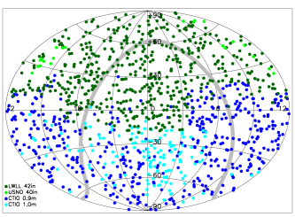
Figure 1: The distribution on the sky of all 1120 M dwarf primaries examined for multiplicity. Different colors indicate the different telescopes that were utilized for the CCD imaging search: royal blue for the CTIO/SMARTS 0.9m, dark green for the Lowell 42in, cyan for the CTIO/SMARTS 1.0m, and bright green for the USNO 40in. The Galactic plane is outlined in gray. Illustrated is the uniformity of the sample in both hemispheres, due in large part to RECONS’ parallax work in the southern hemisphere.

2.2 Sample Selection Biases

We describe here how the sample selection process could bias the result of our survey.

We note that our sample is volume-limited, not volume-complete. If we assume the 188 M dwarf systems in our sample that lie within 10 pc comprise a volume-complete sample and extrapolate to 25 pc assuming a uniform stellar density, we expect 2938 M dwarf systems to lie within 25 pc.

We cross-matched our sample of M dwarf primaries to the recently available parallaxes from the Gaia Data Release 2 (DR2) (Gaia Collaboration et al., 2016, 2018) and found that 90% (1008 primaries) had Gaia parallaxes that placed them within 25 pc. Four percent fell outside of 25 pc with a Gaia DR2 parallax. The remaining 6% (69 primaries) were not found to have a Gaia DR2 parallax, but 47 (4%) are known to be in multiple systems with separations between the components on the order of or less than 1″. Nine of these 47 multiple systems are within the ten parsec horizon. A few of the remaining 22 that are not currently known to be multiple are definitively nearby, but have high proper motion (e.g., GJ 406) or are bright (e.g., GJ 411). We do not make any corrections to our sample based on this comparison because it is evident that a sample of stars surveyed for stellar multiplicity based on the Gaia DR2 would neglect binaries. We look forward, however, to the Gaia DR3 which will include valuable multiplicity information.

Figure 2 shows the distribution of the apparent $I$ magnitudes of the red dwarfs surveyed, with a peak at $I$ = 8.5–9.5. Because brighter objects are generally targeted for parallax measurements before fainter objects for which measurements are more difficult, 85% of the sample is made up of bright stars ($I<$ 12.00), introducing an implicit Malmquist bias. As unresolved multiple systems are usually over-luminous, this survey’s outcomes are biased toward a larger multiplicity rate.

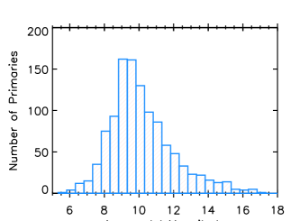
Figure 2: The distribution of $I-$band magnitudes of our sample of 1120 M dwarfs known to lie within 25 pc, illustrating that most (85%) of the target stars are brighter than $I$ = 12.

We have also required the error on the published trigonometric parallax to be $\leq$10 mas in order to limit the sample to members that are reliably within 25 pc. Therefore, it is possible that binaries were missed, as perturbations on the parallax due to an unseen companion can increase the parallax error. Forty-five M dwarf systems with YPC or HIP parallaxes were eliminated from the sample due to their large parallax errors. We cross-checked these 45 targets against the Gaia DR2 with a search radius of 3′, to mitigate the positional offset of these typically high proper motion stars. Twenty-nine were returned with parallaxes by Gaia, 19 of which remained within our chosen 25 pc distance horizon. Four of these 19 had close companions detected by Gaia. If we assumed that the 16 non-detections were all multiple systems and all within 25 pc, the sample size would increase to 1155, and the multiplicity rate would increase by 0.9%. We do not include any correction due to this bias. We note that the parallaxes measured as a result of RECONS’ astrometry program, roughly one-third of the sample, would not factor into this negative bias, as all of these data were examined and stars with astrometric perturbations due to unseen companions flagged.

Additionally, there is mass missing within 25 pc in the form of M dwarf primaries (Winters et al., 2015). However, because the multiplicity rates decrease as a function of primary mass (see §6.1.3 and Figure 19), the percentages of ‘missing’ multiple systems in each mass bin are effectively equal. Based on the 10 pc sample, as above, we expect 969 M dwarfs more massive than 0.30 M_⊙ within 25 pc, but have 506 in our sample. The MR of 28.2% for the estimated 463 missing systems results in 131 (14%) missing multiples in this primary mass subset. We expect 1109 M dwarfs with primaries 0.15 $-$ 0.30 M_⊙ within 25 pc, but have 402 in our sample. The MR of 21.4% for the estimated 707 missing systems results in 151 (14%) missing multiples in this primary mass subset. Finally, we expect 859 M dwarfs with primaries 0.075 $-$ 0.15 M_⊙ within 25 pc, but have 212 in our sample. The MR of 16.0% for the estimated 647 missing systems results in 104 (12%) missing multiples in this primary mass subset. Therefore, we do not include a correction for this bias.

Table 3: Astrometry Data

Name	R.A.	Decl.	$\mu$	P.A.	Ref	$\pi$	$\sigma_{\pi}$	# $\pi$	Ref
	(hh:mm:ss)	(dd:mm:ss)	(″yr-1 )	(deg)		(mas)	(mas)
(1)	(2)	(3)	(4)	(5)	(6)	(7)	(8)	(9)	(10)
GJ 1001ABC	00 04 36.45	$-$40 44 02.7	1.636	159.7	71	77.90	2.04	2	15,68
GJ 1	00 05 24.43	$-$37 21 26.7	6.106	112.5	28	230.32	0.90	2	68,69
LHS 1019	00 06 19.19	$-$65 50 25.9	0.564	158.7	72	59.85	2.64	1	69
GJ 1002	00 06 43.19	$-$07 32 17.0	2.041	204.0	39	213.00	3.60	1	68
GJ 1003	00 07 26.71	$+$29 14 32.7	1.890	127.0	38	53.50	2.50	1	68
LHS 1022	00 07 59.11	$+$08 00 19.4	0.546	222.0	38	44.00	6.30	1	68
L 217-28	00 08 17.37	$-$57 05 52.9	0.370	264.0	40	75.17	2.11	1	73
HIP 687	00 08 27.29	$+$17 25 27.3	0.110	233.8	28	45.98	1.93	1	69
G 131-26AB	00 08 53.92	$+$20 50 25.4	0.251	194.4	53	54.13	1.35	1	53
GJ 7	00 09 04.34	$-$27 07 19.5	0.715	079.7	72	43.61	2.56	2	68,69
LEHPM 1-255	00 09 45.06	$-$42 01 39.6	0.271	096.7	72	53.26	1.51	1	73

Note. — The first 10 lines of this Table are shown to illustrate its form and content.

References. — (1) Andrei et al. (2011); (2) Anglada-Escudé et al. (2012); (3) Bartlett et al. (2017); (4) Benedict et al. (1999); (5) Benedict et al. (2000); (6) Benedict et al. (2001); (7) Benedict et al. (2002); (8) Biller & Close (2007); (9) Costa et al. (2005); (10) Costa et al. (2006); (11) Dahn et al. (2002); (12) Deacon & Hambly (2001); (13) Deacon et al. (2005b); (14) Deacon et al. (2005a); (15) Dieterich et al. (2014); (16) Dupuy & Liu (2012); (17) Fabricius & Makarov (2000); (18) Faherty et al. (2012); (19) Falin & Mignard (1999); (20) Gatewood et al. (1993); (21) Gatewood et al. (2003); (22) Gatewood (2008); (23) Gatewood & Coban (2009); (24) Henry et al. (1997); (25) Henry et al. (2006); (26) Henry et al. (2018); (27) Hershey & Taff (1998); (28) Høg et al. (2000); (29) Ianna et al. (1996); (30) Jao et al. (2005); (31) Jao et al. (2011); (32) Jao et al. (2017); (33) Khovritchev et al. (2013); (34) Lèpine & Shara (2005); (35) Lèpine et al. (2009); (36) Lurie et al. (2014); (37) Luyten (1979a); (38) Luyten (1979b); (39) Luyten (1980a); (40) Luyten (1980b); (41) Martin & Mignard (1998); (42) Martinache et al. (2007); (43) Martinache et al. (2009); (44) Monet et al. (2003); (45) Pokorny et al. (2004); (46) Pourbaix et al. (2003); (47) Pravdo et al. (2006); (48) Pravdo & Shaklan (2009); (49) RECONS (in prep); (50) Reid et al. (2003); (51) Riedel et al. (2010); (52) Riedel et al. (2011); (53) Riedel et al. (2014); (54) Riedel et al. (2018); (55) Schilbach et al. (2009); (56) Schmidt et al. (2007); (57) Shakht (1997); (58) Shkolnik et al. (2012); (59) Smart et al. (2007); (60) Smart et al. (2010); (61) Söderhjelm (1999); (62) Subasavage et al. (2005a); (63) Subasavage et al. (2005b); (64) Teegarden et al. (2003); (65) Teixeira et al. (2009); (66) Tinney et al. (1995); (67) Tinney (1996); (68) van Altena et al. (1995); (69) van Leeuwen (2007); (70) von Braun et al. (2011); (71) Weis (1999); (72) Winters et al. (2015); (73) Winters et al. (2017).

2.3 Optical and Infrared Photometry

Existing $VRI$ photometry for many of the M dwarfs in the sample was culled from the literature, much of which has been presented previously for the southern M dwarfs in Winters et al. (2011, 2015, 2017); however, a number of M dwarfs in the sample had no published reliable optical photometry available. As part of the effort to characterize the M dwarfs in the survey, new absolute photometry in the Johnson-Kron-Cousins $V_{J}R_{KC}I_{KC}$ filters was acquired for 81, 3, and 49 stars at the CTIO/SMARTS 0.9m, CTIO/SMARTS 1.0m, and Lowell 42in telescopes, respectively, and is presented here for the first time. Identical observational methods were used at all three sites. As in previous RECONS efforts, standard star fields from Graham (1982), Bessel (1990), and/or Landolt (1992, 2007, 2013) were observed multiple times each night to derive transformation equations and extinction curves. In order to match those used by Landolt, apertures 14$\arcsec$ in diameter were used to determine the stellar fluxes, except in cases where close contaminating sources needed to be deblended. In these cases, smaller apertures were used and aperture corrections were applied. Further details about the data reduction procedures, transformation equations, etc., can be found in Jao et al. (2005), Winters et al. (2011), and Winters et al. (2015).

In addition to the 0.9m, 1.0m, and 42in observations, three stars were observed at the United States Naval Observatory (USNO) Flagstaff Station 40in telescope. Basic calibration frames, bias and sky flats in each filter are taken either every night (bias) or over multiple nights in a run (sky flats) and are applied to the raw science data. Standard star fields from Landolt (2009, 2013) were observed at multiple airmasses between $\sim$1.0 and $\sim$2.1 each per night to calculate extinction curves. All instrumental magnitudes, both for standards and science targets, are extracted by fitting spatially-dependent point spread functions (PSFs) for each frame using Source Extractor (SExtractor (Bertin & Arnouts, 1996) and PSFEx (Bertin, 2011), with an aperture diameter of 14″. Extensive comparisons of this technique to basic aperture photometry have produced consistent results in uncrowded fields.

Optical and infrared photometry for the 1448 components of the 1120 M dwarf systems is presented in Table 2.3, where available. $JHK_{s}$ magnitudes were extracted from 2MASS (Skrutskie et al., 2006) and confirmed by eye to correspond to the star in question during the blinking survey. Included are the names of the M dwarfs (column 1), the number of known components in the systems (2), J2000.0 coordinates (3, 4), $VRI$ magnitudes (5, 6, 7), the number of observations and/or references (8), the 2MASS $JHK_{s}$ magnitudes (9, 10, 11), and the photometric distance estimate. Next are listed the $\Delta$$V$ magnitudes between stellar companions and primaries (12), the deblended $V$ magnitudes $V_{db}$ (13), and estimated masses for each component (14). Components of multiple systems are noted with a capital letter (A,B,C,D,E) after the name in the first column. If the names of the components are different, the letters identifying the primary and the secondary are placed within parentheses, e.g., LHS1104(A) and LHS1105(B). If the star is a companion in a multiple system, ‘0’ is given in column (2). ‘J’ for joint photometry is listed with each blended magnitude. Brown dwarf companions are noted by a ‘BD’ next to the ‘0’ in column 2, and often do not have complete photometry, if any.

Table 4: Photometry Data

Name	# Obj	R.A.	Decl.	$V_{J}$	$R_{KC}$	$I_{KC}$	# nts/ref	$J$	$H$	$K_{s}$	$\pi_{ccd}$	$\sigma_{\pi}$	$\Delta$$V$	$V_{db}$	Mass
		(dd:mm:ss)	(hh:mm:ss)	(mag)	(mag)	(mag)		(mag)	(mag)	(mag)	(pc)	(pc)	(mag)	(mag)	(M⊙)
(1)	(2)	(3)	(4)	(5)	(6)	(7)	(8)	(9)	(10)	(11)	(12)	(13)	(14)	(15)	(16)
GJ1001B	0BD	00 04 34.87	$-$40 44 06.5	22.77J	19.04J	16.67J	/10	13.11J	12.06J	11.40J	$\cdots$	$\cdots$	$\cdots$	$\cdots$	$\cdots$
GJ1001C	0BD	00 04 34.87	$-$40 44 06.5	$\cdots$	$\cdots$	$\cdots$	$\cdots$	$\cdots$	$\cdots$	$\cdots$	$\cdots$	$\cdots$	$\cdots$	$\cdots$	$\cdots$
GJ1001A	3	00 04 36.45	$-$40 44 02.7	12.83	11.62	10.08	/40	8.60	8.04	7.74	12.5	1.9	$\cdots$	12.83	0.234
GJ0001	1	00 05 24.43	$-$37 21 26.7	8.54	7.57	6.41	/4	5.33	4.83	4.52	5.6	0.9	$\cdots$	8.54	0.411
LHS1019	1	00 06 19.19	$-$65 50 25.9	12.17	11.11	9.78	/21	8.48	7.84	7.63	16.6	2.6	$\cdots$	12.17	0.335
GJ1002	1	00 06 43.19	$-$07 32 17.0	13.84	12.21	10.21	/40	8.32	7.79	7.44	5.4	1.0	$\cdots$	13.84	0.116
GJ1003	1	00 07 26.71	$+$29 14 32.7	14.16	13.01	11.54	/37	10.22	9.74	9.46	36.0	7.0	$\cdots$	14.16	0.203
LHS1022	1	00 07 59.11	$+$08 00 19.4	13.09	12.02	10.65	/37	9.39	8.91	8.65	28.9	5.2	$\cdots$	13.09	0.311
L217-028	1	00 08 17.37	$-$57 05 52.9	12.13	11.00	9.57	/40	8.21	7.63	7.40	13.2	2.0	$\cdots$	12.13	0.293
HIP000687	1	00 08 27.29	$+$17 25 27.3	10.80	9.88	8.93	/35	7.81	7.17	6.98	18.5	3.2	$\cdots$	10.80	0.582

Note. — The first 10 lines of this Table are shown to illustrate its form and content.

Note. — A ‘J’ next to a photometry value indicates that the magnitude is blended due to one or more close companions. A ‘]’ next to the photometric distance estimate indicates that the joint photometry of the multiple system was used to calculate the distance estimate, which is thus likely underestimated. A ’u’ following the photometry reference indicates that we present an update to previously presented RECONS photometry.

Note. — ^a $2MASS$ magnitude error greater than 0.05 mags; ^b An assumption was made regarding the $\Delta$mag; ^c A conversion to $\Delta$$V$ was done from a reported magnitude difference in another filter; ^d Photometry in SOAR filters and not converted to Johnson-Kron-Cousins system; ^e Barbieri et al. (1996); ^f Benedict et al. (2000); ^g Benedict et al. (2016); ^h Henry et al. (1999); ⁱ Henry et al. (1999); Tamazian et al. (2006); ^j Ségransan et al. (2000); ^k Delfosse et al. (1999a); ^l Díaz et al. (2007); ^m Duquennoy & Mayor (1988); ⁿ Herbig & Moorhead (1965); ^o Photometry for ‘AC’, instead of for the ‘B’ component, was mistakenly reported in Davison et al. (2015).

References. — (1) this work; (2) Bartlett et al. (2017); (3) Benedict et al. (2016); (4) Bessel (1990); (5) Bessell (1991); (6) Costa et al. (2005); (7) Costa et al. (2006); (8) Dahn et al. (2002); (9) Davison et al. (2015); (10) Dieterich et al. (2014); (11) Harrington & Dahn (1980); (12) Harrington et al. (1993); (13) Henry et al. (2006); (14) Henry et al. (2018); (15) Høg et al. (2000); (16) Hosey et al. (2015); (17) Jao et al. (2005); (18) Jao et al. (2011); (19) Jao et al. (2017); (20) Koen et al. (2002); (21) Koen et al. (2010); (22) Lèpine et al. (2009); (23) Lurie et al. (2014); (24) Reid et al. (2002); (25) Riedel et al. (2010); (26) Riedel et al. (2011); (27) Riedel et al. (2014); (28) Riedel et al. (2018); (29) Weis (1984); (30) Weis (1986); (31) Weis (1987); (32) Weis (1988); (33) Weis (1991b); (34) Weis (1991a); (35) Weis (1993); (36) Weis (1994); (37) Weis (1996); (38) Weis (1999); (39) Winters et al. (2011); (40) Winters et al. (2015); (41) Winters et al. (2017).

For new photometry reported here, superscripts are added to the references indicating which telescope(s) was used to acquire the $VRI$ photometry: ‘09’ for the CTIO/SMARTS 0.9m, ‘10’ for the CTIO/SMARTS 1.0m, ‘40’ for the USNO 40in, and ‘42’ for the Lowell 42in. If the $\Delta$$V$ is larger than 3, the magnitude of the primary is treated as unaffected by the companion(s). All masses are estimated from the absolute $V$ magnitude, which has been calculated from the deblended $V$ magnitude for each star in column (13), the parallax in Table 2.2, and the empirical mass-luminosity relations of Benedict et al. (2016). If any type of assumption or conversion was made regarding the $\Delta$$V$ (as discussed in §5.3.1), it is noted.

As outlined in Winters et al. (2011), photometric errors at the 0.9m are typically 0.03 mag in $V$ and 0.02 mag in $R$ and $I$. To verify the Lowell 42in data, Table 2.3 presents photometry for four stars observed at the Lowell 42in and at the CTIO/SMARTS 0.9m, as well as six stars with $VRI$ from the literature. Results from the 42in and 0.9m match to 0.06 mag, except for the $R$ magnitude of GJ 1167, which can be attributed to a possible flare event observed at the time of observation at the 42in, as the $V$ and $I$ magnitudes are consistent. This object is, in fact, included in a flare star catalog of UV Cet-type variables (Gershberg et al., 1999). An additional six stars were observed by Weis, and the photometry matches to within 0.08 mag for all six objects, and typically to 0.03 mag. Given our typical 1$\sigma$ errors of at most 0.03 mag for $VRI$, we find that the Lowell 42in data have differences of 2$\sigma$ or less in 28 of the 30 cases shown in Table 2.3.

Table 5: Overlapping Photometry Data

Name	($V-K$)	$V_{J}$	$R_{KC}$	$I_{KC}$	# obs	tel/ref
	(mag)	(mag)	(mag)	(mag)
2MA J0738$+$2400	4.86	12.98	11.81	10.35	1	42in
		12.98	11.83	10.35	2	0.9m
G 43-2	4.76	13.23	12.08	10.67	1	42in
		13.24	12.07	10.66	2	0.9m
2MA J1113$+$1025	5.34	14.55	13.27	11.63	1	42in
		14.50	13.21	11.59	2	0.9m
GJ 1167	5.59	14.16	12.67	11.10	1	42in
		14.20	12.82	11.11	1	0.9m
LTT 17095A	4.22	11.12	10.12	9.00	1	42in
		11.11	10.11	8.94	…	1
GJ 15B	5.12	11.07	9.82	8.34	2	42in
		11.06	9.83	8.26	…	3
GJ 507AC	3.96	9.52	8.56	7.55	1	42in
		9.52	8.58	7.55	…	3
GJ 507B	4.64	12.15	11.06	9.66	1	42in
		12.12	11.03	9.65	…	3
GJ 617A	3.64	8.59	7.68	6.85	1	42in
		8.60	7.72	6.86	…	3
GJ 617B	4.67	10.74	9.67	8.29	1	42in
		10.71	9.63	8.25	…	2

References. — (1) Weis (1993); (2) Weis (1994); (3) Weis (1996).

3 The Searches and Detected Companions

Several searches were carried out on the 1120 nearby M dwarfs in an effort to make this the most comprehensive investigation of multiplicity ever undertaken for stars that dominate the solar neighborhood. Information about the surveys is collected in Tables 6–12, including a statistical overview of the individual surveys in Table 6. Note that the number of detections includes confirmations of previously reported multiples in the literature. Specifics about the Blink Survey are listed in Table 7. Telescopes used for the CCD Imaging Survey in Table 8, while detection limit information for the CCD Imaging Survey is presented in Tables 9 and 10. Results for confirmed multiples are collected in Table 3.2.2, whereas candidate, but as yet unconfirmed, companions are listed in Table 3.3.2.

We report the results of each search here; overall results are presented in §5.

Table 6: Companion Search Technique Statistics

Technique	Separation	Searched	Searched	Detected
	(″)	(#)	(%)	(#)
Image Blinking	5–300	1110	99	64
CCD Imaging	2–10	1120	100	44
RECONS Perturbations	$<$ 2	324	29	39
HR Diagram Elevation	$<$ 2	1120	100	11
Distance Mismatches	$<$ 2	1112	99	37
Hipparcos Flags	$<$ 2	460	41	31
Literature/WDS Search	all	1120	100	290
Individual companions	TOTAL	1120	100	310

Table 7: Blink Survey Information

Filter	Epoch Span	DEC Range	Mag. Limit	$\Delta$$\lambda$
	(yr)	(deg)	(mag)	(Å)
$B_{J}$ (IIIaJ)	1974 - 1994	all-sky	$\sim$20.5	3950 - 5400
$R_{59F}$ (IIIaF)	1984 - 2001	all-sky	$\sim$21.5	5900 - 6900
$I_{IVN}$ (IVN)	1978 - 2002	all-sky	$\sim$19.5	6700 - 9000
$E_{POSS-I}$ (103aE)	1950 - 1957	$-$20.5 $<$ $\delta$ $<$ $+$05	$\sim$19.5	6200 - 6700
$I_{KC}$	2010 - 2014	all sky	$\sim$17.5	7150 - 9000

3.1 Wide-Field Blinking Survey: Companions at 5–300″

Because most nearby stars have large proper motions, images of the stars taken at different epochs were blinked for common proper motion (CPM) companions with separations of 5–300″. A wide companion would have a similar proper motion to its primary and would thus appear to move in the same direction at the same speed across the sky. Archival SuperCOMOS $B_{J}R_{59F}I_{IVN}$ photographic plate images 10′ $\times$ 10′ in size were blinked using the Aladin interface of the Centre de Donneès astronomiques de Strasbourg (CDS) to detect companions at separations greater than $\sim$5″. These plates were taken from 1974–2002 and provide up to 28 years of temporal coverage, with typical epoch spreads of at least 10 years. Information for the images blinked is given in Table 7, taken from Morgan (1995), Subasavage (2007), and the UK Schmidt webpage. Candidates were confirmed to be real by collecting $VRI$ photometry and estimating photometric distances using the suite of relations in Henry et al. (2004); if the distances of the primary and candidate matched to within the errors on the distances, the candidate was deemed to be a physical companion. In addition to recovering 63 known CPM companions, one new CPM companion (2MA0936-2610C) was discovered during this blinking search, details of which are given in §4.1. No comprehensive search for companions at angular separations larger than 300″ was conducted.

3.1.1 Blink Survey Detection Limits

The CPM search had two elements that needed to be evaluated in order to confidently identify objects moving with the primary star in question: companion brightness and the size of each system’s proper motion.

A companion would have to be detectable on at least two of the three photographic plates in order to notice its proper motion, so any companion would need to be brighter than the magnitude limits given in Table 7 in at least two images. Because the search is for stellar companions, it is only necessary to be able to detect a companion as faint as the faintest star in the sample, effectively spectral type M9.5 V at 25 pc. The two faintest stars in the sample are DEN 0909-0658, with $VRI$ = 21.55, 19.46, 17.18 and RG0050-2722 with $VRI$ = 21.54, 19.09, 16.65. The $B$ magnitudes for these stars are both fainter than the mag$\sim$20.5 limit of the $B$ plate, and thus neither star was detected in the $B$ image; however, their $R$ and $I$ magnitudes are both brighter than the limits of those plates and the stars were identified in both the $R$ and $I$ images. Ten other objects are too faint to be seen on the $B$ plate, but as is the case with DEN0909-0658 and RG0050-2722, all are bright enough for detection in the $R$ and $I$ images.

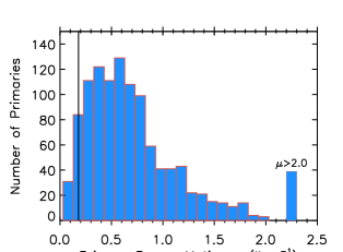
Figure 3: Histogram of the proper motion of the primary (or single) component in each system, with the vertical line indicating $\mu$ $=$ 0$\farcs$18 yr^-1, the canonical lower proper motion limit of Luyten’s surveys. The majority (95%) have proper motions, $\mu$, larger than 0$\farcs$18 yr^-1.

The epoch spread between the plates also needed to be large enough to detect the primary star moving in order to then notice a companion moving in tandem with it. As shown in the histogram of proper motions in Figure 3, most of the survey stars move faster than 0$\farcs$18 yr^-1, the historical cutoff of Luyten’s proper motion surveys. Hence, even a 10-year baseline provides 1$\farcs$8 of motion, our adopted minimum proper motion detection limit, easily discerned when blinking plates. However, 58 of the stars in the survey ($\sim$5% of the sample) have $\mu$ $<$ 0$\farcs$18 yr^-1, with the slowest star having $\mu$ $=$ 0$\farcs$03 yr^-1; for this star, to detect a motion of 1$\farcs$8 the epoch spread would need to be 60 years. For 18 stars with Decl $-$20 $<$ $\delta$ $<$ $+$5^∘, the older POSS-I plate (taken during 1950–1957) was used for the slow-moving primaries. This extended the epoch spread by 8–24 years, enabling companions for these 18 stars to be detected, leaving 40 slow-moving stars to search.

The proper motions of 151 additional primaries were not initially able to be detected confidently because the epoch spread of the SuperCOSMOS plates was less than 5 years. These 151 stars, in addition to the 40 stars with low $\mu$ mentioned above that were not able to be blinked using the POSS plates, were compared to our newly-acquired $I-$band images taken during the CCD Imaging Survey, extending the epoch spread by almost twenty years in some cases. Wherever possible, the SuperCOSMOS $I-$band image was blinked with our CCD $I-$band image, but sometimes a larger epoch spread was possible with either the $B-$ or $R-$band plate images. In these cases, the plate that provided the largest epoch spread was used. In order to upload these images to Aladin to blink with the archival SuperCOSMOS images, World Coordinate System (WCS) coordinates were added to the header of each image so that the two images could be aligned properly. This was done using SExtractor for the CTIO/SMARTS 0.9m and the USNO 40in images and the tools at Astrometry.net for the Lowell 42in and the CTIO/SMARTS 1.0m images.

After using the various techniques outlined above to extend the image epoch spreads, 1110 of 1120 stars were sucessfully searched in the Blink Survey for companions. In ten cases, either the primary star’s proper motion was still undetectable, the available CCD images were taken under poor sky conditions and many faint sources were not visible, or the frame rotations converged poorly. A primary result from this Blink Survey is that in the separation regime from 10–300″, where the search is effectively complete, we find a multiplicity rate of 4.7% (as discussed in §5.2). Thus, we estimate that only 0.5 CPM stellar companions (10 $\ast$ 4.7%) with separations 10–300″ were missed due to not searching ten stars during the Blinking Survey.

3.2 CCD Imaging Survey: Companions at 2–10″

To search for companions with separations 2–10″, astrometry data were obtained at four different telescopes: in the northern hemisphere, the Hall 42in telescope at Lowell Observatory and the USNO 40in telescope, both in Flagstaff, AZ, and in the southern hemisphere, the CTIO/SMARTS 0.9m and 1.0m telescopes, both at Cerro Tololo Inter-American Observatory in Chile. Each M dwarf primary was observed in the $I_{KC}$ filter with integrations of 3, 30, and 300 seconds in order to reveal stellar companions at separations 2–10″. This observational strategy was adopted to reveal any close equal-magnitude companions with the short 3-second exposures, while the long 300-second exposures would reveal faint companions with masses at the end of the main sequence. The 30-second exposures were taken to bridge the intermediate phase space. Calibration frames taken at the beginning of each night were used for typical bias subtraction and dome flat-fielding using standard $IRAF$ procedures.

Table 8: Telescopes Utilized for CCD Imaging Search and $VRI$ Photometry

Telescope	FOV	Pixel Scale	# Nights	# Objects
Lowell 42in	22.3′ $\times$ 22.3′	0$\farcs$327 px-1	21	508
USNO 40in	22.9′ $\times$ 22.9′	0$\farcs$670 px-1	1	22
CTIO/SMARTS 0.9m	13.6′ $\times$ 13.6′	0$\farcs$401 px-1	16	442
CTIO/SMARTS 1.0m	19.6′ $\times$ 19.6′	0$\farcs$289 px-1	8	148

Technical details for the cameras and specifics about the observational setups and numbers of nights and stars observed at each telescope are given in Table 8. The telescopes used for the imaging campaign all have primary mirrors roughly 1m in size and have CCD cameras that provide similar pixel scales. Data from all telescopes were acquired without binning pixels. The histogram in Figure 4 illustrates the seeing measured for the best images of each star surveyed at the four different telescopes. Seeing conditions better than 2″ were attained for all but one star, GJ 507, with some stars being observed multiple times. While the 0.9m has a slightly larger pixel scale than the 1.0m and the 42in, as shown in Figure 4, the seeing was typically better at that site, allowing for better resolution. Only 22 primaries (fewer than 2% of the survey) were observed at the USNO 40in, so we do not consider the coarser pixel scale to have significantly affected the survey. Overall, the data from the four telescopes used were of similar quality and the results could be combined without modification.

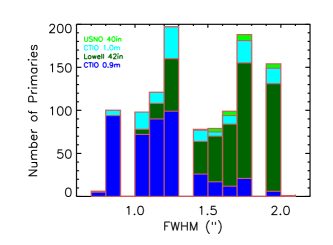
Figure 4: The seeing FWHM measured for target star frames used in the $I-$band CCD imaging search. The four different telescopes used are represented as royal blue for the CTIO/SMARTS 0.9m, dark green for the Lowell 42in, cyan for the CTIO/SMARTS 1.0m, and bright green for the USNO 40in. Note the generally superior seeing conditions for targets observed at the 0.9m.

A few additional details of the observations are worthy of note:

$\bullet$ A total of 442 stars were observed at the CTIO/SMARTS 0.9m telescope, where consistently good seeing, telescope operation, and weather conditions make observations at this site superior to those at the other telescopes used, as illustrated in Figure 4.

$\bullet$ While being re-aluminized in December 2012, the primary mirror at the Lowell 42in was dropped and damaged. The mask that was installed over the damaged mirror as a temporary fix resulted in a PSF flare before a better mask was installed that slightly improved the PSF. Of the 508 stars observed for astrometry at Lowell, 457 were observed before the mishap and 51 after.

$\bullet$ $I-$band images at both the Lowell 42in and CTIO/SMARTS 1.0m suffer from fringing, the major cause of which is night sky emission from atmospheric OH molecules. This effect sometimes occurs with back-illuminated CCDs at optical wavelengths longer than roughly 700 nm where the light is reflected several times between the internal front and back surfaces of the CCD, creating constructive and destructive interference patterns, or fringing (Howell, 2000, 2012). In order to remove these fringes, $I-$band frames from multiple nights with a minimum of saturated stars in the frame were selected, boxcar smoothed, and then average-combined into a fringe map. This fringe map was then subtracted from all $I-$band images using a modified IDL code originally crafted by Snodgrass & Carry (2013).

Four new companions were discovered during this portion of the survey. Details on these new companions are given in §4.1. In each case, archival SuperCOSMOS plates were blinked to eliminate the possibility that new companions were background objects. We detected 32 companions with separations 2–10″, as well as 12 companions with $\rho<$ 2″, including the four noted above.

3.2.1 CCD Imaging Survey Detection Limits

The $M_{I}$ range of the M dwarf sequence is roughly 8 magnitudes ($M_{I}=$ 6.95 — 14.80 mag, specifically, for our sample). Therefore, an analysis of the detection limits of the CCD imaging campaign was done for objects with a range of $I$ magnitudes at $\rho$ $=$ 1–5″ and at $\Delta$mags $=$ 0 – 8 in one-magnitude increments for different seeing conditions at the two main telescopes where the bulk (85%) of the stars were imaged: the CTIO/SMARTS 0.9m and the Lowell 42in. While the companion search in the CCD frames extended to 10″, sources were detected even more easily at separations 5 – 10″ than at 5″, so it was not deemed necessary to perform the analysis for the larger separations.

Because the apparent $I-$band magnitudes for the stars in the sample range from 5.32–17.18 (as shown in Figure 2), objects with $I-$band magnitudes of approximately 8, 12, and 16 were selected for investigation. Only 88 primaries (7.8% of the sample) have $I<$ 8, so it was not felt necessary to create a separate set of simulations for these brighter stars. The stars used for the detection limit analysis are listed in Table 9 with their $I$ magnitudes, the FWHM at which they were observed and at which telescope, and any relevant notes.

Table 9: Stars Used for Imaging Search Detection Limit Study

Name	$I$	FWHM	Tel	Note
	(mag)	(arcsec)
GJ 285	8.24	0.8	0.9m
LP 848-50AB	12.47J	0.8	0.9m	$\rho$AB $<$2″
SIP 1632-0631	15.56	0.8	0.9m
L 32-9A	8.04	1.0	0.9m	$\rho$AB $=$ 22$\farcs$40
SCR 0754-3809	11.98	1.0	0.9m
BRI 1222-1221	15.59	1.0	0.9m
GJ 709	8.41	1.0	42in
GJ 1231	12.08	1.0	42in
Reference Star	16 (scaled)	1.0	42in
GJ 2060AB	7.83J	1.5	0.9m	$\rho$AB $=$ 0$\farcs$485
2MA 2053-0133	12.46	1.5	0.9m
Reference Star	16 (scaled)	1.5	0.9m
GJ 109	8.10	1.5	42in
LHS 1378	12.09	1.5	42in
2MA 0352+0210	16.12	1.5	42in
Reference Star	8 (scaled)	1.8	0.9m
SCR 2307-8452	12.00	1.8	0.9m
Reference Star	16 (scaled)	1.8	0.9m
GJ 134	8.21	1.8	42in
LHS 1375	12.01	1.8	42in
SIP 0320-0446AB	16.37	1.8	42in	$\rho$AB $<$0$\farcs$33
GJ 720A	8.02	2.0	42in	$\rho$AB $=$ 112$\farcs$10
LHS 3005	11.99	2.0	42in
2MA 1731+2721	15.50	2.0	42in

Note. — The ‘J’ on the $I-$band magnitudes of LP 848-50AB and GJ 2060AB indicates that the photometry includes light from the companion. The other sub-arcsecond binary, SIP 0320-0446AB, has a brown dwarf companion that does not contribute significant light to the photometry of its primary star.

Each of the selected test stars was analyzed in seeing conditions of 1$\farcs$0, 1$\farcs$5, and 1$\farcs$8, but because the seeing at CTIO is typically better than that at Anderson Mesa, we were able to push to 0$\farcs$8 for the 0.9m, and had to extend to 2$\farcs$0 for the Lowell 42in. These test stars were verified to have no known detectable companions within the 1–5″ separations explored in this part of the project. We note that one of the targets examined for the best resolution test, LP 848-050AB, has an astrometric perturbation due to an unseen companion at an unknown separation, but that in data with a FWHM of 0.8″, the two objects were still not resolved. As the detection limit determination probes separations 1–5″, using this star does not affect the detection limit analysis. The other binaries used all had either larger or smaller separations than the 1–5″ regions explored, effectively making them point sources.

The $IDL$ shift task was used to shift and add the science star as a proxy for an embedded companion, scaled by a factor of 2.512 for each magnitude difference. In cases where the science star was saturated in the frame, a reference star was selected from the shorter exposure taken in similar seeing in which the science star was not saturated. Its relative magnitude difference was calculated so that it could be scaled to the desired brightness in the longer exposure, and then it was embedded for the analysis. In all cases, the background sky counts were subtracted before any scaling was done.

Figure 5: Detection Limits for the CTIO/SMARTS 0.9m: Contour plots for L 32-9A, with $I=$ 8.04 in 1$\farcs$0 seeing conditions for an embedded companion at $\rho$ $=$ 1–5″ with $\Delta$mags $=$ 0–8. The Y, N, and M labels indicate $yes$, $no$, or $maybe$ for whether or not the embedded companion is detectable. The 3-second exposure was used for $\Delta$mags $=$ 0–3, the 30-second exposure was used for $\Delta$mags $=$ 4–5, and the 300-second exposure was used for $\Delta$mags $=$ 6–8. Thirty-five simulated companions were detected, seven were undetectable, and three were possibly detected.

Figure 6: Detection Limits for the CTIO/SMARTS 0.9m: Contour plots for SCR 0754-3809, with $I=$ 11.98 mag at 1$\farcs$0 seeing conditions for an embedded companion at $\rho$ $=$ 1$-$5″ with $\Delta$mags $=$ 0–4. The Y, N, and M labels indicate $yes$, $no$, or $maybe$ for whether or not the embedded companion is detectable. The 30-second exposure was used for $\Delta$mags $=$ 0, 1, 2, and the 300-second exposure was used for $\Delta$mags $=$ 3, 4. Twenty-two simulated companions were detected, one was undetectable, and two were possibly detected.

Figure 7: Detection Limits for the CTIO/SMARTS 0.9m: Contour plots for BRI 1222-1221, with $I=$ 15.59 mag at 1$\farcs$0 seeing conditions for an embedded companion at $\rho$ $=$ 1$-$5″ with $\Delta$mags $=$ 0. The Y, N, and M labels indicate $yes$, $no$, or $maybe$ for whether or not the embedded companion is detectable. The 300-second exposure was used. All 5 simulated companions were detected.

Stars with $I$ = 8 were searched for companion sources in $IRAF$ via radial and contour plots using the 3-second exposure to probe $\Delta$$I$ $=$ 0, 1, 2, 3, the 30-second exposure for $\Delta$$I$ $=$ 4, 5, and the 300-second exposure for $\Delta$$I$ $=$ 6, 7, 8. Similarly, twelfth magnitude stars were probed at $\Delta$$I$ $=$ 0, 1, 2, 3 using the 30-second exposure and at $\Delta$$I$ $=$ 4 with the 300-second frame. Finally, the 300-second exposure was used to explore the regions around the sixteenth magnitude objects for evidence of a stellar companion at $\Delta$$I$ $=$ 0.

In total, 600 contour plots were made using $IDL$ and inspected by eye. A subset of 75 example plots for stars with $I$ = 8.04, 11.98, and 15.59 observed in seeing conditions of 1$\farcs$0 at the 0.9m are shown in Figures 5 - 7. The ‘Y’, ‘N’, and ‘M’ labels in each plot indicate $yes$, $no$, or $maybe$ for whether or not the injected synthetic companion was detectable by eye at the separation, magnitude, and seeing conditions explored. As can be seen, the target star with $I$ = 8.04 is highly saturated in the frames used for $\Delta$$I$ greater than 4. Overall, the companion can be detected in 62 of the 75 simulations, not detected in eight cases, and possibly detected in five more cases. The conditions in which the companion remains undetected in some cases are at small $\rho$ and at $\Delta$$I$ $>$ 4, typically around bright stars. Note that these images do not stand alone — contour plots for target stars are also compared to plots for other stars in the frames, allowing an additional check to determine whether or not the star in question is multiple.

Table 10: Imaging Search Detection Limit Summary

Seeing	Yes	No	Maybe	Yes	No	Maybe
Conditions	(#)	(#)	(#)	(#)	(#)	(#)
		0.9m			42in
FWHM $=$ 0$\farcs$8	64	8	3	$\cdots$	$\cdots$	$\cdots$
$I$ $=$ 8 mag	36	7	2	$\cdots$	$\cdots$	$\cdots$
$I$ $=$ 12 mag	23	1	1	$\cdots$	$\cdots$	$\cdots$
$I$ $=$ 16 mag	5	$\cdots$	$\cdots$	$\cdots$	$\cdots$	$\cdots$
FWHM $=$ 1$\farcs$0	62	8	5	60	12	3
$I$ $=$ 8 mag	35	7	3	34	8	3
$I$ $=$ 12 mag	22	1	2	21	4	$\cdots$
$I$ $=$ 16 mag	5	$\cdots$	$\cdots$	5	$\cdots$	$\cdots$
FWHM $=$ 1$\farcs$5	58	12	5	55	12	8
$I$ $=$ 8 mag	33	9	3	33	6	6
$I$ $=$ 12 mag	20	3	2	17	6	2
$I$ $=$ 16 mag	5	$\cdots$	$\cdots$	5	$\cdots$	$\cdots$
FWHM $=$ 1$\farcs$8	50	18	7	52	14	9
$I$ $=$ 8 mag	28	13	4	29	10	6
$I$ $=$ 12 mag	18	5	2	19	4	2
$I$ $=$ 16 mag	4	$\cdots$	1	4	$\cdots$	1
FWHM $=$ 2$\farcs$0	$\cdots$	$\cdots$	$\cdots$	46	17	12
$I$ $=$ 8 mag	$\cdots$	$\cdots$	$\cdots$	24	12	9
$I$ $=$ 12 mag	$\cdots$	$\cdots$	$\cdots$	18	5	2
$I$ $=$ 16 mag	$\cdots$	$\cdots$	$\cdots$	4	$\cdots$	1
TOTAL	234	46	20	213	55	32

The full range of $\Delta$$I$ for the M dwarf sequence is roughly eight magnitudes, so $\Delta$$I>$ 8 represents detections of early L dwarf and brown dwarf companions. There were no companions detected with $\Delta$$I$ $>$ 8 around the brighter stars in the simulations, indicating that this survey was not sensitive to these types of faint companions at separations 1–5″ around the brightest M dwarfs in the sample, although they would be detected around many of the fainter stars (none were found).

Table 10 presents a summary of the results of the detections of the embedded companions. Overall, the simulated companions were detected 75% of the time for all brightness ratios on both telescopes, were not detected 17% of the time, and were possibly detected in 9% of the simulations. For the simulations of bright stars with $I=$ 8, 70% of the embedded companions were detected. For stars with $I=$ 12, companions were detected in 79% of the time, and for the faint stars with $I=$ 16, companions were detected in 93% of the cases tested. At $\rho$ $=$ 1″, the embedded companions were detected in 28% of cases, not detected in 52% of cases, and possibly detected in 20% of cases. Thus, we do not claim high sensitivity at separations this small. In total, for $\rho$ $\geq$ 2″, we successfully detected the simulated companions 86% of the time, did not detect them 8% of the time, and possibly detected them 6% of the time.

We note that this study was not sensitive to companions with large $\Delta$mags at separations $\sim$1 — 2″ from their primaries. While the long exposure $I-$band images obtained during the direct imaging campaign would likely reveal fainter companions at $\rho$ $\sim$2 — 5″, the saturation of some of the observed brighter stars creates a CCD bleed along columns in the direction in which the CCDs read out. Faint companions located within $\sim$1— 2″ of their primaries, but at a position angle near 0^∘ or 180^∘ would be overwhelmed by the CCD bleed of the saturated star and not be detected. We do not include any correction due to this bias, as it mostly applies to companions at separations $<$ 2″ from their primaries, below our stated detection limit sensitivity.

Figure 8: Log-linear plot of $\Delta$$I$ vs. angular separation to illustrate the observational limits of our Blinking and CCD Imaging Surveys. Solid black points indicate known companions that were confirmed, while the new companions discovered during our searches are shown as larger blue points.

3.2.2 Detection Limits Summary

Figure 8 illustrates detected companions in the Blinking and CCD Imaging Surveys, providing a comparison for the detection limits derived here. We note that the largest $\Delta$$I$ detected was roughly 6.0 mag (GJ 752B), while the largest angular separation detected was 295″ (GJ 49B).

Figure 9 indicates the coverage curves for our two main surveys as a function of projected linear separation. Using the angular separation limits of each survey (2 — 10″  for the imaging survey and 5 — 300″ for the blinking survey) and the trigonometric distances of each object to determine the upper and lower projected linear separation limit for each M dwarf primary in our sample, we show that either the imaging or blinking survey would have detected stellar companions at projected distances of 50 - 1000 AU for 100% of our sample.

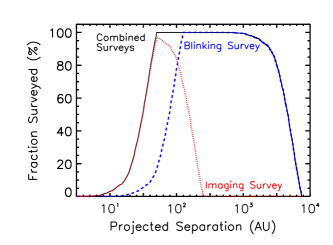
Figure 9: The fraction of our sample surveyed as a function of log-projected linear separation. The curve for the imaging campaign is shown as a red dotted line, while the blinking campaign coverage is shown as a blue dashed line. The solid black line indicates the combined coverage of the two campaigns. We show that our surveys are complete for stellar companions at projected linear separations of roughly 50 - 1000 AU, 75% complete at separations 40 - 3000 AU, and 50% complete at separations 30 - 4000 AU.

Table 11: Multiplicity Information for Sample

Name	# Obj	Map	RA	DEC	$\rho$	$\theta$	Year	Technique	Ref	$\Delta$mag	Filter	Ref
			(hh:mm:ss)	(dd:mm:ss)	(″)	(deg)				(mag)
GJ 1001	0	BC	00 04 34.87	$-$40 44 06.5	0.087	048	2003	HSTACS	40	0.01	222	40
GJ 1001	3	A-BC	00 04 36.45	$-$40 44 02.7	18.2	259	2003	visdet	40	9.91	$V_{J}$	1
G 131-26	2	AB	00 08 53.92	$+$20 50 25.4	0.111	170	2001	AO det	13	0.46	H	13
GJ 11	2	AB	00 13 15.81	$+$69 19 37.2	0.859	089	2012	lkydet	62	0.69	i’	62
LTT 17095	2	AB	00 13 38.74	$+$80 39 56.8	12.78	126	2001	visdet	103	3.63	$V_{J}$	1
GJ 1005	2	AB	00 15 28.06	$-$16 08 01.8	0.329	234	2002	HSTNIC	30	2.42	$V_{J}$	9
2MA 0015-1636	2	AB	00 15 58.07	$-$16 36 57.8	0.105	090	2011	AO det	18	0.06	H	18
L 290-72	2	AB	00 16 01.99	$-$48 15 39.3	$<$1	…	2007	SB1	117	…	…	…
GJ 1006	2	AB	00 16 14.62	$+$19 51 37.6	25.09	059	1999	visdet	103	0.94	$V_{J}$	111
GJ 15	2	AB	00 18 22.88	$+$44 01 22.7	35.15	064	1999	visdet	103	2.97	$V_{J}$	1

Note. — The first 10 lines of this Table are shown to illustrate its form and content.

Note. — The codes for the techniques and instruments used to detect and resolve systems are: AO det — adaptive optics; astdet — detection via astrometric perturbation, companion often not detected directly; astorb — orbit from astrometric measurements; HSTACS — Hubble Space Telescope’s Advanced Camera for Surveys; HSTFGS — Hubble Space Telescope’s Fine Guidance Sensors; HSTNIC — Hubble Space Telescope’s Near Infrared Camera and Multi-Object Spectrometer; HSTWPC — Hubble Space Telescope’s Wide Field Planetary Camera 2; lkydet — detection via lucky imaging; lkyorb — orbit from lucky imaging measurements; radorb — orbit from radial velocity measurements; radvel — detection via radial velocity, but no SB type indicated; SB (1, 2, 3) — spectroscopic multiple, either single-lined, double-lined, or triple-lined; spkdet — detection via speckle interferometry; spkorb — orbit from speckle interferometry measurements; visdet — detection via visual astrometry; visorb — orbit from visual astrometry measurements

References. — (1) this work; (2) Allen & Reid (2008); (3) Al-Shukri et al. (1996); (4) Balega et al. (2007); (5) Balega et al. (2013); (6) Bartlett et al. (2017); (7) Benedict et al. (2000); (8) Benedict et al. (2001); (9) Benedict et al. (2016); (10) Bergfors et al. (2010); (11) Bessel (1990); (12) Bessell (1991); (13) Beuzit et al. (2004); (14) Biller et al. (2006); (15) Blake et al. (2008); (16) Bonfils et al. (2013); (17) Bonnefoy et al. (2009); (18) Bowler et al. (2015); (19) Burningham et al. (2009); (20) Chanamé & Gould (2004); (21) Cortes-Contreras et al. (2014); (22) Cvetković et al. (2015); (23) Daemgen et al. (2007); (24) Dahn et al. (1988); (25) Davison et al. (2014); (26) Dawson & De Robertis (2005); (27) Delfosse et al. (1999a); (28) Delfosse et al. (1999b); (29) Díaz et al. (2007); (30) Dieterich et al. (2012); (31) Docobo et al. (2006); (32) Doyle & Butler (1990); (33) Duquennoy & Mayor (1988); (34) Femenía et al. (2011); (35) Forveille et al. (2005); (36) Freed et al. (2003); (37) Fu et al. (1997); (38) Gizis (1998); (39) Gizis et al. (2002); (40) Golimowski et al. (2004); (41) Harlow (1996); (42) Harrington et al. (1985); (43) Hartkopf et al. (2012); (44) Heintz (1985); (45) Heintz (1987); (46) Heintz (1990); (47) Heintz (1991); (48) Heintz (1992); (49) Heintz (1993); (50) Heintz (1994); (51) Henry et al. (1999); (52) Henry et al. (2006); (53) Henry et al. (2018); (54) Herbig & Moorhead (1965); (55) Horch et al. (2010); (56) Horch et al. (2011a); (57) Horch et al. (2012); (58) Horch et al. (2015b); (59) Ireland et al. (2008); (60) Janson et al. (2012); (61) Janson et al. (2014a); (62) Janson et al. (2014b); (63) Jao et al. (2003); (64) Jao et al. (2009); (65) Jao et al. (2011); (66) Jenkins et al. (2009); (67) Jódar et al. (2013); (68) Köhler et al. (2012); (69) Kürster et al. (2009); (70) Lampens et al. (2007); (71) Law et al. (2006); (72) Law et al. (2008); (73) Leinert et al. (1994); (74) Lèpine et al. (2009); (75) Lindegren et al. (1997); (76) Luyten (1979a); (77) Malo et al. (2014); (78) Martín et al. (2000); (79) Martinache et al. (2007); (80) Martinache et al. (2009); (81) Mason et al. (2009); (82) Mason et al. (2018); (83) McAlister et al. (1987); (84) Montagnier et al. (2006); (85) Nidever et al. (2002); (86) Pravdo et al. (2004); (87) Pravdo et al. (2006); (88) Reid et al. (2001); (89) Reid et al. (2002); (90) Reiners & Basri (2010); (91) Reiners et al. (2012); (92) Riddle et al. (1971); (93) Riedel et al. (2010); (94) Riedel et al. (2014); (95) Riedel et al. (2018); (96) Salim & Gould (2003); (97) Schneider et al. (2011); (98) Scholz (2010); (99) Ségransan et al. (2000); (100) Shkolnik et al. (2010); (101) Shkolnik et al. (2012); (102) Siegler et al. (2005); (103) Skrutskie et al. (2006); (104) Tokovinin & Lépine (2012); (105) van Biesbroeck (1974); (106) van Dessel & Sinachopoulos (1993); (107) Wahhaj et al. (2011); (108) Ward-Duong et al. (2015); (109) Weis (1991b); (110) Weis (1993); (111) Weis (1996); (112) Winters et al. (2011); (113) Winters et al. (2017); (114) Winters et al. (2018); (115) Woitas et al. (2003); (116) Worley & Mason (1998); (117) Zechmeister et al. (2009).

3.3 Searches at Separations $\leq$ 2″

In addition to the blinking and CCD imaging searches, investigations for companions at separations smaller than 2″ were possible using a variety of techniques, as detailed below in Sections §3.3.1–3.3.4. The availability of accurate parallaxes for all stars and of $VRIJHK$ photometry for most stars made possible the identification of overluminous red dwarfs that could be harboring unresolved stellar companions. Various subsets of the sample were also probed using long-term astrometric data for stars observed during RECONS’ astrometry program, as well as via data reduction flags indicating astrometric signatures of unseen companions for stars observed by Hipparcos.

3.3.1 Overluminosity via Photometry: Elevation Above the Main Sequence

Figure 10: Observational HR Diagram for 1120 M dwarf primaries, with $M_{V}$ plotted versus $(V-K)$ color. All primaries are plotted as black points. Overplotted are known close multiples with separations less than 5″ having blended photometry (red points), known subdwarfs (open green squares), and known young objects (open cyan diamonds). Error bars are shown in gray, and are smaller than the points, in most cases. The large $K$ magnitude errors for four objects (GJ0408, GJ0508.2, LHS3472, and LP876-026AB) have been omitted for clarity. As expected, known multiples with merged photometry are often elevated above the middle of the distribution. The 11 stars suspected to be new unresolved multiples due to their elevated positions relative to the main sequence are indicated with open blue circles. The ten stars suspected to be new unresolved multiples due to their distance mismatches from Figure 11 are indicated with open blue triangles. Note that the candidate multiples detected by main sequence elevation are mostly mid-to-late type M dwarfs, while the suspected multiples identified by the distance mismatch technique are primarily early-type M dwarfs.

Accurate parallaxes and $V$ and $K$ magnitudes for stars in the sample allow the plotting of the observational HR Diagram shown in Figure 10, where $M_{V}$ and the $(V-K)$ color are used as proxies for luminosity and temperature, respectively. Unresolved companions that contribute significant flux to the photometry cause targets to be overluminous, placing them above the main sequence. Known multiples with separations $<$ 5″  are evident as points clearly elevated above the presumed single stars on the main sequence, and merge with a few young objects. Subdwarfs are located below and to the left of the singles, as they are old, metal-poor, and underluminous at a given color. Eleven candidate multiples lying among the sequence of known multiples have been identified by eye via this HR Diagram. These candidates are listed in Table 3.3.2 and are marked in Figures 10 and 11. Note that these candidates are primarily mid-to-late M dwarfs. Known young stars and subdwarfs were identified during the literature search and are listed in Tables 3.4.2 and 3.4.3, along with their identifying characteristics. More details on these young and old systems are given in Sections 3.4.2 and 3.4.3.

3.3.2 Overluminosity via Photometry: Trigonometric & CCD Distance Mismatches

Figure 11: A comparison of distance estimates from $VRIJHK$ photometry vs. distances using $\pi_{trig}$ for 1091 of the M dwarf primaries in the sample. The 29 stars with photometric distances $>$ 30 pc are not included in this plot. Errors on the distances are noted in gray. The diagonal solid line represents 1:1 agreement in distances, while the dashed lines indicate the 15% uncertainties associated with the CCD distance estimates from Henry et al. (2004). The dash-dot line traces the location where the trigonometric distance exceeds the photometric estimate by a factor of $\sqrt{2}$, corresponding to an equal-luminosity/mass pair of stars. Known unresolved multiples with blended photometry are indicated with red points. The 11 candidate unresolved multiples from the HR Diagram in Figure 10 are enclosed with open blue circles. The ten new candidates that may be unresolved multiples from this plot are enclosed with open blue triangles.

Because both $VRI$ and 2MASS $JHK$ photometry are now available for nearly the entire sample, photometric distances based on CCD photometry (ccddist) were estimated and compared to the accurate trigonometric distances (trigdist) available from the parallaxes. Although similar in spirit to the HR Diagram test discussed above that uses $V$ and $K$ photometry, all of the $VRIJHK$ photometry is used for each star to estimate the ccddist via the technique described in Henry et al. (2004), thereby leveraging additional information. As shown in Figure 11, suspected multiples that would otherwise have been missed due to the inner separation limit (2″) of our main imaging survey can be identified due to mismatches in the two distances. For example, an unresolved equal magnitude binary would have an estimated ccddist closer by a factor of $\sqrt{2}$ compared to its measured trigdist. Unresolved multiples with more than two components, e.g., a triple system, could be even more overluminous, as could young, multiple systems. By contrast, cool subdwarfs are underluminous and therefore, their photometric distances are overestimated.

With this method, 50 candidate multiples were revealed with ccddists that were $\sqrt{2}$ or more times closer than their trigdists. Of these, 40 were already known to have at least one close companion (36 stars), or to be young (four stars), verifying the technique. The remaining ten are new candidates, and are listed in Table 3.3.2.

Table 12: Suspected Multiple Systems

Name	# Stars	RA	DEC	Flag	Reference
		(hh:mm:ss)	(dd:mm:ss)
GJ1006A	3?	00 16 14.62	$+$19 51 37.6	dist	1
HIP006365	2?	01 21 45.39	$-$46 42 51.8	X	3
LHS1288	2?	01 42 55.78	$-$42 12 12.5	X	3
GJ0091	2?	02 13 53.62	$-$32 02 28.5	X	3
GJ0143.3	2?	03 31 47.14	$+$14 19 17.9	X	3
BD-21-01074A	4?	05 06 49.47	$-$21 35 03.8	dist	1
GJ0192	2?	05 12 42.22	$+$19 39 56.5	X	3
GJ0207.1	2?	05 33 44.81	$+$01 56 43.4	possSB	4
SCR0631-8811	2?	06 31 31.04	$-$88 11 36.6	elev	1
LP381-004	2?	06 36 18.25	$-$40 00 23.8	G	3
SCR0702-6102	2?	07 02 50.36	$-$61 02 47.7	elev,pb?	1,1
LP423-031	2?	07 52 23.93	$+$16 12 15.0	elev	1
SCR0757-7114	2?	07 57 32.55	$-$71 14 53.8	dist	1
GJ1105	2?	07 58 12.70	$+$41 18 13.4	X	3
LHS2029	2?	08 37 07.97	$+$15 07 45.6	X	3
LHS0259	2?	09 00 52.08	$+$48 25 24.7	elev	1
GJ0341	2?	09 21 37.61	$-$60 16 55.1	possSB	4
GJ0367	2?	09 44 29.83	$-$45 46 35.6	X	3
GJ0369	2?	09 51 09.63	$-$12 19 47.6	X	3
GJ0373	2?	09 56 08.68	$+$62 47 18.5	possSB	4
GJ0377	2?	10 01 10.74	$-$30 23 24.5	dist	1
GJ1136A	3?	10 41 51.83	$-$36 38 00.1	X,possSB	3,4
GJ0402	2?	10 50 52.02	$+$06 48 29.4	X	3
LHS2520	2?	12 10 05.59	$-$15 04 16.9	dist	1
GJ0465	2?	12 24 52.49	$-$18 14 32.3	pb?	2
DEN1250-2121	2?	12 50 52.65	$-$21 21 13.6	elev	1
GJ0507.1	2?	13 19 40.13	$+$33 20 47.7	X	3
GJ0540	2?	14 08 12.97	$+$80 35 50.1	X	3
2MA1507-2000	2?	15 07 27.81	$-$20 00 43.3	dist,elev	1
G202-016	2?	15 49 36.28	$+$51 02 57.3	G	3
LHS3129A	3?	15 53 06.35	$+$34 45 13.9	dist	1
GJ0620	2?	16 23 07.64	$-$24 42 35.2	G	3
GJ1203	2?	16 32 45.20	$+$12 36 45.9	X	3
LP069-457	2?	16 40 20.65	$+$67 36 04.9	elev	1
LTT14949	2?	16 40 48.90	$+$36 18 59.9	X	3
HIP083405	2?	17 02 49.58	$-$06 04 06.5	X	3
LP044-162	2?	17 57 15.40	$+$70 42 01.4	elev	1
LP334-011	2?	18 09 40.72	$+$31 52 12.8	X	3
SCR1826-6542	2?	18 26 46.83	$-$65 42 39.9	elev	1
LP044-334	2?	18 40 02.40	$+$72 40 54.1	elev	1
GJ0723	2?	18 40 17.83	$-$10 27 55.3	X	3
HIP092451	2?	18 50 26.67	$-$62 03 03.8	possSB	4
LHS3445A	3?	19 14 39.15	$+$19 19 03.7	dist	1
GJ0756	2?	19 21 51.42	$+$28 39 58.2	X	3
LP870-065	2?	20 04 30.79	$-$23 42 02.4	dist	1
GJ1250	2?	20 08 17.90	$+$33 18 12.9	dist	1
LEHPM2-0783	2?	20 19 49.82	$-$58 16 43.0	elev	1
GJ0791	2?	20 27 41.65	$-$27 44 51.9	X	3
LHS3564	2?	20 34 43.03	$+$03 20 51.1	X	3
GJ0811.1	2?	20 56 46.59	$-$10 26 54.8	X	3
L117-123	2?	21 20 09.80	$-$67 39 05.6	X	3
HIP106803	2?	21 37 55.69	$-$63 42 43.0	X	3
LHS3748	2?	22 03 27.13	$-$50 38 38.4	X	3
G214-014	2?	22 11 16.96	$+$41 00 54.9	X	3
GJ0899	2?	23 34 03.33	$+$00 10 45.9	X	3
GJ0912	2?	23 55 39.77	$-$06 08 33.2	X	3

References. — (1) this work; (2) Heintz (1986); (3) Lindegren et al. (1997); (4) Reiners et al. (2012).

Note. — Flag Description: dist means that the ccddist is at least $\sqrt{2}$ times closer than the trigdist due to the object’s overluminousity; elev means that the object is elevated above the main sequence in the HR Diagram in Figure 10 due to overluminosity; possSB means that the object has been noted as a possible spectroscopic binary by Reiners et al. (2012); pb? indicates that a possible perturbation was noted. The the single letters are Hipparcos reduction flags as follows: $G$ is an acceleration solution where a component might be causing a variation in the proper motion; $V$ is for Variability-Induced Movers, where one component in an unresolved binary could be causing the photocenter of the system to be perturbed; $X$ is for a stochastic solution, where no reliable astrometric parameters could be determined, and which may indicate an astrometric binary.

3.3.3 RECONS Perturbations

A total of 324 red dwarfs in the sample have parallax measurements by RECONS, with the astrometric coverage spanning 2–16 years. This number is slightly higher than the 308 parallaxes listed in Table 2, due to updated and more accurate RECONS parallax measurements that improved upon YPC parallaxes with high errors. The presence of a companion with a mass and/or luminosity different from the primary causes a perturbation in the photocenter of the system that is evident in the astrometric residuals after solving for the proper motion and parallax. This is the case for 39 of the observed systems, which, although sometimes still unseen, are listed as confirmed companions in Table 3.2.2, where references are given. Because 13 of these 39 stars with perturbations were detected during the course of this project, we note them as new discoveries, although they were first reported in other papers (e.g., Bartlett et al., 2017; Jao et al., 2017; Winters et al., 2017; Henry et al., 2018; Riedel et al., 2018). A new companion to USN2101$+$0307 was reported in Jao et al. (2017). We present here the nightly mean astrometric residual plots in RA and DEC for this star (shown in in Figure 12), which exhibits a perturbation due to its unseen companion. This system is discussed in more detail in §4.1.

This is the only technique used in this companion search that may have revealed brown dwarf companions. None of the companions have been resolved, so it remains uncertain whether the companion is a red or brown dwarf. As we noted in Winters et al. (2017), the magnitude of the perturbation in the photocenter of the system, $\alpha$, follows the relation $\alpha$ = (B $-$ $\beta$)$a$, where B is the fractional mass M_B/(M_A $+$ M_B), $\beta$ is the relative flux expressed as $(1+10^{0.4\Delta m})^{-1}$, and $a$ is the semi-major axis of the relative orbit of the two components (van de Kamp, 1975). The degeneracy between the mass ratio/flux difference and the scaling of the photocentric and relative orbits results in an uncertainty in the nature of the companion. We are able to assume that the companion is a red dwarf if the system is overluminous, which is the case for eight of these systems. Therefore, we conservatively assume that all the companions are red dwarfs. These particular systems are high priority targets for high-resolution, speckle observations through our large program on the Gemini telescopes that is currently in-progress, with a goal of resolving and characterizing the companions.

Figure 12: Nightly mean astrometric residual plots in RA and DEC for USN2101$+$0307. The astrometric signature of the system’s proper motion and parallax has been removed, leaving clear indication that an unseen companion is perturbing the position of the primary star.

3.3.4 Hipparcos Reduction Flags

All 460 stars in the sample with Hipparcos parallaxes were searched for entries in the Double and Multiple Systems Annex (DMSA) (Lindegren et al., 1997) of the original Hipparcos Catalog to reveal any evidence of a companion. Of these 460 stars, 229 have a parallax measured only by Hipparcos, while 231 also have a parallax measurement from another source. Various flags exist in the DMSA that confirm or infer the presence of a companion: C — component solutions where both components are resolved and have individual parallaxes; G — acceleration solutions, i.e., due to variable proper motions, which could be caused by an unseen companion; O — orbits from astrometric binaries; V — Variability-Induced Movers (VIMs), where the variability of an unresolved companion causes the photocenter of the system to move or be perturbed; X — stochastic solutions, for which no astrometric parameters could be determined and which may indicate that the star is actually a short-period astrometric binary.

Most of the AFGK systems observed by Hipparcos that have flags in the DMSA have been further examined or re-analyzed by Pourbaix et al. (2003, 2004), Platais et al. (2003), Jancart et al. (2005), Frankowski et al. (2007), Horch et al. (2002, 2011a, 2011b, 2015a, 2017); however, few of the M dwarf systems have been investigated to date. Stars with C and O flags were often previously known to be binary, are considered to be confirmed multiples, and are included in Table 3.2.2. We found that G, V, or X flags existed for 31 systems in the survey — these suspected multiples are listed in Table 3.3.2.

3.4 Literature Search

Finally, a literature search was carried out by reviewing all 1120 primaries in SIMBAD and using the available bibliography tool to search for papers reporting additional companions. While SIMBAD is sometimes incomplete, most publications reporting companions are included. Papers that were scrutinized in detail include those reporting high resolution spectroscopic studies (typically radial velocity planet searches or rotational velocity results that might report spectroscopic binaries), parallax papers that might report perturbations, high resolution imaging results, speckle interferometry papers, and other companion search papers. A long list of references for multiple systems found via the literature search is included in Table 3.2.2.

In addition, the Washington Double Star Catalogue (WDS), maintained by Brian Mason, was used extensively to find publications with information on multiple systems. Regarding the WDS, we note that: (1) not all reported companions are true physical members of the system with which they are listed, and (2) only resolved companions (i.e., no spectroscopic or astrometric binaries) are included in the catalog. Thus, care had to be taken when determining the true number of companions in a system. Information pertaining to a star in the WDS was usually only accessed after it was already known that the system was multiple and how many components were present in the system, so this was not really troublesome. However, the WDS sometimes had references to multiplicity publications that SIMBAD had not listed. Thus, the WDS proved valuable in identifying references and the separations, magnitude differences, and other information included in Table 3.2.2.

Finally, all of the multiple systems were cross-checked against the Gaia DR2 through the $Aladin$ interface. Thirty-two known multiple systems had positional data, but no parallax, while fourteen known systems were not found. Of the 575 stellar components presented in this sample, 133 were not found to have separate data points. The majority of these companions are located at sub-arcsecond angular separations from their primaries, with a rare few having separations 1 – 3″. An additional 15 companions had unique coordinates, but no individual parallax or proper motion. We anticipate that future Gaia data releases will provide some of the currently missing information for these low-mass multiple systems.

Information for all multiple systems (including brown dwarf components) is presented in Table 3.2.2, with n-1 lines for each system, where n is the total number of components in the system. For example, a quadruple system will have three lines of information that describe the system. The name is followed by the number of components in the system and the configuration map of the components detailed in that line of the Table. If the line of data pertains to higher order systems containing component configurations for sub-systems (e.g., ‘BC’ of a triple system), the number of components noted will be ‘0’, as the full membership of the system will already have been noted in the line of data containing the ‘A’ component. These data are followed by epoch J2000.0 coordinates, the angular separation ($\rho$) in arcseconds, the position angle ($\theta$) in degrees measured East of North, the year of the measurement, the code for the technique used to identify the component, and the reference. We assign a separation of $<$1″ for all astrometric and spectroscopic binaries (unless more information is available) and/or to indicate that a companion has been detected, but not yet resolved. We note that where orbit determinations from the literature are reported, the semimajor axis, $a$, is listed instead of $\rho$. If $a$ was not reported in the reference given, it was calculated from the period and the estimated masses of the components in question via Kepler’s Third Law.

The final three columns give a magnitude difference ($\Delta$mag) between the components indicated by the configuration map, the filter used to measure this $\Delta$mag, and the reference for this measurement. Photometry from photographic plates is denoted by ‘V*’. In many cases, there are multiple separation and $\Delta$mag measurements available in the literature from different groups using different techniques. An exhaustive list of these results is beyond the scope of this work; instead, a single recent result for each system is listed. In a few cases, the position angles and/or $\Delta$mag measurements are not available. We discuss how these systems are treated in §5.3.1.

3.4.1 Suspected Companions

Forty-nine singles suspected to be doubles were revealed during this survey, three of which (GJ 912, GJ 1250, and SCR 1826-6542) have so far been confirmed with continuing follow-up observations. An additional five doubles are suspected to be triples, yielding a current total of 54 suspected additional companions (only one companion per system in all cases) listed in Table 3.3.2, but not included in Table 3.2.2. Systems in Table 3.3.2 are listed with the suspected number of components followed by a question mark to indicate the system’s suspect status, followed by J2000.0 coordinates, a flag code for the reason a system is included as having a candidate companion, and the reference. Notes to the table give detailed descriptions of the flags. Among the 56 suspected companions, 31 are from the Hipparcos DMSA, in which they are assigned G, V, or X flags. A number of primaries that were suspected to be multiple due to either an underestimated ccddist or an elevated position on the HR diagram were found through the literature search to have already been resolved by others and have been incorporated into Table 3.2.2 and included in the analysis as confirmed companions. There remain 21 systems in Table 3.3.2 with ccddist values that do not match their trigonometric parallax distances and/or that are noticeably elevated above the main sequence that have not yet been confirmed. A few more systems had other combinations of indicators that they were multiple, e.g., an object with a perturbation might also have a distance mismatch. Six stars were reported as suspected binaries in the literature. GJ 207.1, GJ 341, GJ 373, GJ 1136A and HIP 92451 were noted by Reiners et al. (2012) as possible spectroscopic binaries, and GJ 465 was identified by Heintz (1986) as a possible astrometric binary. These are listed in Table 3.3.2. We reiterate that none of these suspected companions have been included in any of the analyses of the previous section or that follow; only confirmed companions have been used.

3.4.2 Young Stellar Objects

Within the solar neighborhood are young moving groups that have contributed members to the multiplicity sample. Within the studied collection are 16 confirmed young M dwarfs, nine of which are known to be multiple, yielding a multiplicity rate of 56$\pm$19%. We note that this result is not statistically robust due to the small number of objects with which it was calculated. Presented in Table 3.4.2 are these known nearby young red dwarfs, with their astrometric data duplicated from Table 2.2. In addition, the tangential velocity $v_{tan}$ is listed, along with the youth indicators, the moving group with which they are associated, and the reference. The youth indicators are as follows: BF — a bona fide and well-known member of a moving group; Li — the presence of lithium; ol — over-luminous. Any member of a multiple system where one component exhibits any of these indicators is also assumed to be young, as in the case of GJ 871.1AB. We note that we do not exclude any of the identified young M dwarf members from our sample. This would arbitrarily bias our sample, as a comprehensive search for these objects in the current sample has not been conducted.

Table 13: Young Members

Name	# objects	RA	DEC	$\mu$	P.A.	Ref	$v_{tan}$	Youth	Moving	Ref
		(hh:mm:ss)	(dd:mm:ss)	(″ yr-1)	(deg)		(km s-1)	Indicator	Group
LTT 10301AB	2	00 50 33.23	$+$24 49 00.9	0.203	101.9	5	11	ol	Argus	3
G 80-21	1	03 47 23.35	$-$01 58 19.8	0.323	147.8	5	25	Li	AB Dor	3
2MA 0414-0906	1	04 14 17.29	$-$09 06 54.3	0.168	325.2	4	19	Li	none	3
LP 776-25	1	04 52 24.42	$-$16 49 22.2	0.243	150.7	2	18	ol	AB Dor	3
GJ 2036AB	2	04 53 31.20	$-$55 51 37.3	0.149	060.6	5	8	BF	AB Dor	3
LP 717-36AB	2	05 25 41.67	$-$09 09 12.6	0.197	164.7	6	19	ol	AB Dor	3
AP COL	1	06 04 52.16	$-$34 33 36.0	0.330	003.6	6	13	Li	Argus	3
CD-35 2722AB	2	06 09 19.22	$-$35 49 31.1	0.057	186.4	4	6	BF	AB Dor	3
GJ 2060ABC	3	07 28 51.37	$-$30 14 49.2	0.212	207.9	5	15	BF	AB Dor	3
G 161-71	1	09 44 54.19	$-$12 20 54.4	0.321	277.1	1	21	ol	Argus	1
GJ 382	1	10 12 17.67	$-$03 44 44.4	0.314	219.0	5	12	ol	AB Dor	3
TWA 22AB	2	10 17 26.91	$-$53 54 26.5	0.149	264.4	6	12	Li	Beta Pic	3
GJ 393	1	10 28 55.56	$+$00 50 27.6	0.950	219.3	5	32	ol	AB Dor	3
GJ 490ABCD	4	12 57 40.26	$+$35 13 30.3	0.307	240.9	5	29	BF	Tuc-Hor	3
GJ 856AB	2	22 23 29.08	$+$32 27 33.1	0.329	129.1	5	24	Li	AB Dor	3
GJ 871.1AB	2	22 44 57.96	$-$33 15 01.7	0.230	123.1	5	25	(Li)	Beta Pic	3
HIP 114066	1	23 06 04.83	$+$63 55 33.9	0.185	108.5	5	21	Li	AB Dor	3

Note. — The youth indicators are as follows: BF — a bona fide and well-known member of a moving group; Li — the presence of lithium; ol — over-luminous.

References. — (1) Bartlett et al. (2017); (2) Høg et al. (2000); (3) Riedel et al. (2017); (4) Shkolnik et al. (2012); (5) van Leeuwen (2007); (6) Winters et al. (2015).

3.4.3 Old, Cool Subdwarfs

There are a small number of old halo members, also known as cool subdwarfs, that happen to be passing through the solar neighborhood. The objects have been identified either spectroscopically or stand out on a Reduced Proper Motion Diagram. Out of the eleven confirmed subdwarf members with trigonometric parallaxes found within 25 pc, only three are multiple systems, resulting in a multiplicity rate of 27$\pm$16%. This is very similar to that of the M dwarf population as a whole (26.8$\pm$1.4%; see §5.2) and in agreement with a larger sample of 62 K and M subdwarfs has been studied by Jao et al. (2009), who found a rate of of 26$\pm$6%. As with the young stars, with such a small number of objects, this result is not statistically robust. The known subdwarfs in our sample are identified in Table 3.4.3. In addition to the astrometric data for each system that have been duplicated from Table 2.2, the calculated tangential velocities $v_{tan}$ and spectral types from the literature are listed. We note that we do not exclude any of the identified M-type subdwarfs from our study. This would arbitrarily bias our sample, as a comprehensive search for these objects in the current sample has not been conducted.

Table 14: Subdwarf Members

Name	# objects	RA	DEC	$\mu$	P.A.	Ref	$v_{tan}$	Spectral	Ref
		(hh:mm:ss)	(dd:mm:ss)	(″ yr-1)	(deg)		(km s-1)	Type
LHS 1490	1	03 02 06.36	$-$39 50 51.9	0.859	221.3	8	58	M5.0 VI	4
GJ 1062	1	03 38 15.70	$-$11 29 13.5	3.033	152.0	7	230	M2.5 VI	3
LHS 189AB	2	04 25 38.35	$-$06 52 37.0	1.204	145.7	2	105	M3.0 VIJ	4
LHS 272	1	09 43 46.16	$-$17 47 06.2	1.439	279.2	5	92	M3.0 VI	3
GJ 455AB	2	12 02 18.08	$+$28 35 14.2	0.791	268.0	7	74	M3.5 VIJ	3
LHS 2852	1	14 02 46.67	$-$24 31 49.7	0.506	315.6	8	41	M2.0 VI	3
LHS 375	1	14 31 38.25	$-$25 25 32.9	1.386	269.0	7	158	M4.0 VI	3
SSSPM J1444-2019	1	14 44 20.33	$-$20 19 25.5	3.507	236.0	6	270	M9.0 VI:	6
GJ 2116	1	15 43 18.33	$-$20 15 32.9	1.173	195.3	8	119	M2.0 VI	1
LHS 3409	1	18 45 52.24	$+$52 27 40.7	0.843	298.0	7	81	M4.5 VI	3
LHS 64AB	2	21 07 55.39	$+$59 43 19.4	2.098	209.0	7	238	M1.5 VIJ	3

References. — (1) Bidelman (1985); (2) Costa et al. (2006); (3) Gizis (1997); (4) Jao et al. (2008); (5) Jao et al. (2011); (6) Schilbach et al. (2009); (7) van Altena et al. (1995); (8) Winters et al. (2015).

3.4.4 Substellar Companions

Because this study focuses on the stellar companions of M dwarfs, it was important to determine which companions were stellar and which were substellar. Dieterich et al. (2014) found that the boundary between stars and brown dwarfs is near the L2.0V spectral type; efforts are underway to determine to what mass this spectral type corresponds. As mentioned in §2, $M_{V}=$ 20.0 and $(V-K)=$ 9.5 were used as cutoffs for the faintest and reddest (and correspondingly least massive) M dwarfs. Analysis of the main sequence in the HR diagram created from the RECONS list of stars and brown dwarfs within 25 pc indicates that $M_{V}=$ 21.5 and $(V-K)=$ 10.3 correspond to spectral type L2.0V, and therefore the end of the stellar main sequence. Thus, for this large statistical study, we consider objects fainter or redder than these limits to be substellar brown dwarfs.

Via the literature search, 18 brown dwarf companions to 15 M dwarf primaries were identified. These are noted in Table 2.3 with a ‘BD’ for the component in the object column (column 2). Although no comprehensive searches have been done for brown dwarfs as companions to the 1120 M dwarfs targeted here (including ours), we note that as presently known, the rate of M dwarf primaries with known brown dwarf companions is 1.3$\pm$0.3%. This is a factor of twenty-one less than the stellar multiplicity rate, considering the stellar and brown dwarf companions detected to date. While more brown dwarf companions will undoubtedly be found in the future, it seems that they are genuinely much rarer than stellar companions. We note that astrometric detection via a perturbation is the only technique used in this survey that was sensitive to brown dwarf companions, and only a few stars (GJ 1215, SCR 1845-6357) have so far been found to be orbited by brown dwarfs via perturbations in data from our astrometric survey at the CTIO/SMARTS 0.9m.

We do not include any brown dwarf companions in the analysis that follows, nor are planetary companions addressed in this work.

4 Notes on Individual Systems

4.1 New Companions

Several new companions were discovered during the surveys, or confirmed after being noticed during the long-term astrometry program at the CTIO/SMARTS 0.9m. They are listed in order of RA. In each case, archival SuperCOSMOS plates were blinked to eliminate the possibility that new companions were background objects.

$\bullet$ GJ 84.1C (0205$-$2804) was found during the imaging survey separated by 1$\farcs$5 from GJ 84.1B at a position angle of 299^∘ and with a $\Delta$$I$ = 0.23 mag, making the system a triple. The SuperCOSMOS $B$ and $R$ plates, taken September 1977 and November 1994, respectively, provide a $\Delta$t of 17.2 years. Blinking these two plates using the $CDS$ Aladin interface showed that the B component, with a proper motion of 0$\farcs$549 yr^-1, moved 9$\farcs$4. Projecting the star’s position forward 17 years to the date of the observation (October 2011) indicates that there was no background star at the position of the B component at that time. Astrometry from the Gaia DR2 confirms our discovery, with reported parallaxes of 38.29$\pm$0.03, 38.51$\pm$0.08, and 38.15$\pm$0.10 mas for the now three components. We therefore consider this star a new member of the system.

$\bullet$ 2MA 0936-2610C (0936$-$2610) During the blinking survey, we detected a new companion to this previously known double star at $\rho$ $=$ 41$\farcs$8, $\theta$ $=$ 315^∘, making this a triple system. The $\Delta$$V$ between the AB pair and the C component is 6.9 mag. There is no Gaia DR2 parallax available for the AB pair, yet, but the trigonometric distance of 18.50$\pm$0.05 pc for the C component (54.04$\pm$0.12 mas; Gaia Collaboration et al., 2018) is in agreement with the ground-based parallax of 53.75$\pm$1.42 mas (18.6 pc; Riedel et al., 2018) of the AB pair. We therefore consider this star a new member of the system.

$\bullet$ UPM 1710-5300B (1710$-$5300) was found during the imaging survey as a companion separated by 1$\farcs$2 from its primary at a position angle of 339^∘, with $\Delta$$I$ = 1.2 mag. The archival $B$ and $R$ plates, taken July 1977 and April 1993, respectively, provide a $\Delta$t of 15.8 years. Blinking these two plates showed that the primary component, with a proper motion of 0$\farcs$207 yr^-1, moved 4$\farcs$1. Projecting the star’s position forward 20 years to the date of the observation (April 2013) indicates that there was no background star of similar brightness at the position of the primary component at that time. Astrometry from the Gaia DR2 confirms our discovery, with reported parallaxes of 45.54$\pm$0.12 and 45.05$\pm$0.15 mas for the two components. We consider this star a new binary system.

$\bullet$ LHS 5348 (1927$-$2811) This binary system discovery was previously reported in Winters et al. (2017) along with its parallax measurement; however, we include it here with updated multiplicity information, as it was discovered during the multiplicity survey. It is separated by 0$\farcs$89 from its primary at a position angle of 283^∘, with $\Delta$$I$ = 2.3 mag. The archival $B$ and $I$ plates, taken September 1976 and July 1996, respectively, provide a $\Delta$t of 19.8 years. Blinking these two plates showed that the primary component, with a proper motion of 0$\farcs$509 yr^-1, moved 10″. Projecting the star’s position forward 17 years to the date of the observation (May 2013) indicates that there was no background star of similar brightness at the position of the primary component at that time. While there are two data points in the Gaia DR2 at the positions of the two components, only one reports a parallax in agreement with the distance of the system. The other has no associated parallax measurement. We nevertheless consider this a new binary system and anticipate that future Gaia data releases will confirm our discovery.

$\bullet$ 2MA 1951-3510B (1951$-$3510) was found during the imaging survey as a companion separated by 1$\farcs$9 from its primary at a position angle of 131^∘, with $\Delta$$I$ = 0.3 mag. The $B$ and $R$ plates, taken July 1976 and September 1990, respectively, provide a $\Delta$t of 14.1 years. Blinking these two plates showed that the primary component, with a proper motion of 0$\farcs$373 yr^-1, moved 5$\farcs$3. Projecting the star’s position forward 23 years to the date of the observation (May 2013) indicates that there was no background star of similar brightness at the position of the primary component at that time. Astrometry from the Gaia DR2 confirms our discovery, with reported parallaxes of 88.20$\pm$0.08 and 88.27$\pm$0.09 mas for the two components (Gaia Collaboration et al., 2018). We consider this a new binary system.

$\bullet$ USN 2101$+$0307 (2101$+$0307) This object shows a clear astrometric perturbation, which was not reported in Jao et al. (2017), although it was noted as a binary. As shown in Figure 12, the orbit has not yet wrapped, with more than ten years of data available for this system. The photometric distance estimate of 13.9$\pm$2.2 pc disagrees marginally with the trigonometric distance of 17.7$\pm$0.6 pc. This indicates that the system is slightly overluminous, which indicates that the companion contributes some light to the system and is therefore likely a star and not a brown dwarf. The companion is not resolved in the Gaia DR2.

4.2 Interesting Systems

There are some systems that require more detail than that given in Table 3.2.2, typically those that constitute more than two components or that are particularly interesting. These are listed here with the first four digits of RA and Decl. in sexagesimal hours and degrees, respectively. Note that below, we adopt the moniker GJ to identify all Gl, GL, and GJ stars, also known as “Gliese” stars.

GJ 2005ABC (0024-2708) This system is a triple, not a quadruple. Upon further analysis of the $HST$-$FGS$ data, the D component reported in Henry et al. (1999) is a false detection and is not real.

GJ 1046AB (0219-3646) The SB companion is a probable brown dwarf with 168.848 day period (Kürster et al., 2008); also described by Zechmeister et al. (2009). Bonfils et al. (2013) also note that the companion is a brown dwarf or sub-stellar in nature.

GJ 109 (0244+2531) This object is tagged as a VIM (Variability-Induced Mover) in the Hipparcos catalog, which could imply duplicity. However, Pourbaix et al. (2003) have shown this to be an incorrect tag in their re-analysis and re-calculation of the $(V-I)$ colors. This object is not included as a candidate multiple.

GJ 165AB (0413+5031) Allen et al. (2007) refer to Gl 165B (what we here call GJ 165B) as an L4 dwarf; however, this is likely a typo for GD 165B, which is reported as a bona fide brown dwarf companion to a white dwarf Kirkpatrick & McCarthy (1994); McLean et al. (2003). The coordinates of GD 165B are $\alpha$ $=$ 14:24:39.09, $\delta$ $=$ $+$09:17:10.4, so it is not the same object as GJ 165B. Kirkpatrick & McCarthy (1994) discuss both Gl 65B and GD 165B. GJ 165AB seems to be a possible equal magnitude binary (Heintz, 1992), while McAlister et al. (1987) provide separation information from speckle observations. These data are noted in Table 3.2.2.

LTT 11399 (0419+3629) Both Worley (1961) and Worley (1962) report that this is a binary with a separation of 6$\farcs$4 at 226^∘. Balega et al. (2007) observed this star using speckle interferometry but were unable to resolve it. It is also marked as having a stochastic solution in Lindegren et al. (1997). Closer inspection and backtracking of its proper motion indicate that the alleged component is a background star. We consider this to be a single star and do not list it in Table 3.3.2.

GJ 273 (Luyten’s Star) (0727$+$0513) This star was reported in Ward-Duong et al. (2015) as having a close companion; however, based on previous observations of this object with myriad methods (IR speckle (Leinert et al., 1997), long-term astrometric monitoring (15.2 yr Gatewood, 2008), high resolution spectroscopy (Nidever et al., 2002; Bonfils et al., 2013), etc.), we conclude that the reported companion is likely an unassociated background object. We treat this object as single.

GJ 289 (0748+2022) Marcy & Benitz (1989) note that Gl 289 (GJ 289) is an SB2, but this is likely a typo for GJ 829, which is noted in Marcy et al. (1987) as being a probable SB2. We did not see reports of GJ 289 being an SB2 noted anywhere else in the literature. We treat GJ 289 as a single object.

GJ 1103 (0751-0000) Reiners et al. (2012) cite Delfosse et al. (1998) for GJ 1103(A) being an SB. However, Delfosse et al. (1998) note only that they exclude GJ 1103 from their sample due to it being a binary. They do not claim that it is an SB. In the LHS Catalog (Luyten, 1979a), where it is listed as LHS 1951, it is advertised to have a companion LHS 1952 with a separation of 3″ at $\theta$ $=$ 78^∘, with component magnitudes of m_R $=$ 13.0 and 15.5, and m_pg $=$ 15.0 and 17.5. We searched for the companion by examining both RECONS astrometry frames, in which the seeing was sometimes 1$\farcs$2 or better; and via the blinking campaign. No companion was found. We conclude that GJ 1103 is single.

GJ 450 (1151$+$3516) This object was reported as a low probability binary candidate with a low velocity amplitude by Young et al. (1987) who measured five epochs of precise radial velocities. However, more recent high resolution observations with ELODIE and SOPHIE over a range of resolutions (R $=$ 40,000 - 75,000) make no mention of this object being multiple (Houdebine, 2010), nor was a companion detected with lucky imaging (Jódar et al., 2013) or with infrared adaptive optics observations (Ward-Duong et al., 2015). We therefore consider this object to be single.

GJ 452 (1153$-$0722) Gould & Chanamé (2004) report a likely white dwarf companion at $\rho$ $=$ 9″ and $\theta$ $=$ 110^∘ that was detected in 1960 by Luyten (1980a). However, blinking SuperCOSMOS plate images (epochs 1984 - 1997) with the 300 second integration taken at the CTIO/SMARTS 0.9m reveals no co-moving companion. Backtracking the proper motion of the star to epoch 1960 places a background star at the appropriate separation and position angle of the reported companion. We thus consider this object to be single.

GJ 1155AB (1216+0258) This object was previously thought to have a white dwarf companion, but Gianninas et al. (2011) report that the white dwarf is actually a misclassified M dwarf. A survey of SDSS objects by Kleinman et al. (2004) did not spectroscopically confirm the companion as a white dwarf. We therefore consider the companion to be an M dwarf.

GJ 465 (1224-1814) Heintz (1986) notes this object may yet be a long-term binary. We note this system as a candidate multiple in Table 3.3.2.

GJ 471 (1231+0848) Poveda et al. (1994) report that this object is a common proper motion companion to the binary GJ 469AB with a separation of 2490″. While the weighted mean trigonometric distances from van Altena et al. (1995) and van Leeuwen (2007) agree within the error bars (73.13$\pm$1.28 mas for GJ 471 versus 74.77$\pm$3.39 mas for GJ 469AB), their proper motions are significantly different: 822 mas yr^-1 at $\theta$ $=$ 231^∘ for GJ 471 versus 685 mas yr^-1 at $\theta$ $=$ 248^∘ for GJ 469AB. Thus, we consider GJ 471 a single star.

GJ 477AB (1235-4556) This object is flagged in the Hipparcos DMSA (Lindegren et al., 1997) as having a stochastic solution, indicating that it is a probable short-period astrometric binary. Zechmeister et al. (2009) note it as an SB1 using VLT$+$UVES, with the companion being low-mass or a brown dwarf. We treat the companion as a stellar component.

GJ 1167 (1309+2859) Jahreiß et al. (2008) note a B component with $\mu$ $=$ 0$\farcs$292 yr^-1, $\theta$ $=$ 234.9^∘, but then note that the two stars are not physically associated, as the photometric distance for B is 190 pc while the trigonometric distance for A is 12 pc. We calculate the ccddist for A to be 14.2 pc. Janson et al. (2012) note that A is single in their survey. We conclude that GJ 1167‘B’ is not a CPM companion to GJ 1167A and that GJ 1167 is a single system.

GJ 541.2AB (1417$+$4526) This system had too small a proper motion (47 mas yr^-1 at a position angle of 109.8^∘; van Leeuwen, 2007) to confirm its secondary component with a separation of 55.2″ at a position angle of 204^∘. Our image, taken in 2013, provided 18 years of coverage when blinked with the 1995 SuperCOSMOS plate, but resulted in the system moving less than an arcsecond during our blinking survey. However, the Gaia DR2 catalog confirms this system as a binary, reporting parallaxes and proper motions for both components that agree both with each other and the HIP parallax of 52.60$\pm$1.25 mas: $\pi$${}_{A}=$ 51.43$\pm$0.03 mas and $\mu$${}_{A}=$ 47.3 mas yr^-1, $\theta$${}_{A}=$ 113^∘; $\pi$${}_{B}=$ 51.74$\pm$0.16 mas and $\mu$${}_{B}=$ 47.8 mas yr^-1, $\theta$${}_{B}=$ 113^∘. We therefore treat this system as binary.

GJ 680 (1735$-$4840) A companion at $\rho=$ 3$\farcs$94, $\theta=$ 323.7^∘ with $\Delta$$H$ $=$ 1.93 mag was reported in Ward-Duong et al. (2015). However, whilst performing PSF photometry in the crowded field in order to deblend the magnitudes of the primary and secondary, we noted that the alleged secondary had not moved with the primary between epochs of photometry taken eighteen months apart. With a proper motion of 462 mas yr^-1, the two stars would have moved a pixel and a half. This was the case with the primary, but not the alleged secondary. Therefore, we deem the companion a background star and not physically associated.

GJ 687 (1736+6820) Montet et al. (2014) cite Jenkins et al. (2009) for the M3.5 companion that they note in their Table 2. But the spectral type of the primary is M3.5. Jenkins et al. (2009) do not note any additional information about a companion.

We find that the WDS lists GJ 687 as the B component to the F5 star HD 160861. The parallax for the F5 star is 11.20 mas (89 pc; van Leeuwen, 2007) which places this object at a much larger distance than the M dwarf, which has $\pi$ $=$ 220.47 mas (4.5 pc; van Altena et al., 1995; van Leeuwen, 2007). It appears that the ‘A’ component, the F5 star (at $\alpha$ $=$ 17:36:42, $\delta$ $=$ $+$68:22:59, compared to $\alpha$ $=$ 17:36:25.9, $\delta$ $=$ $+$68:20:20 for GJ 687) is an SB, for which the measurement by McAlister et al. (1987) pertains. Tokovinin (1992) notes GJ 687 as both an astrometric and speckle binary in the table in that paper named ‘Long-period spectroscopic binaries’. But this, too, is likely for the F dwarf. The companion is deemed to be optical, and we consider GJ 687 to be single.

LTT 15769 (1945+3223) This system is listed as double in the Hipparcos DMSA (Lindegren et al., 1997) with $\rho$ $=$ 12$\farcs$76, $\theta$ $=$ 339^∘ with a quality code of ‘D’, indicating an uncertain solution. Blinking the SuperCOSMOS $R$ plate image with an $I$-band image taken with the Lowell 42in image results in an epoch difference of nineteen years and reveals the motion of the primary, but not that of the bright ‘secondary’ with a $\Delta$$H_{p}$ of 2.3 mag. We thus refute this low probability companion and deem the system ‘single.’

GJ 793 (2030$+$6527) Weis (1991b) lists this object in the ‘Rejected Pairs’ table (Table 5) and note that the alleged companion is not listed in either the Luyten or Giclas catalogs. The SuperCOSMOS photographic plates had an epoch spread of only one year, so we used the 300-second image taken during our imaging campaign at the Lowell 42in to blink with the SuperCOSMOS $I-$band archival image. This resulted in a $\delta$t $=$ 20 yr. No common proper motion companion was detected. We confirm that this object is single.

GJ 873 (2246$+$4420) This object was reported by van de Kamp & Worth (1972) to be an astrometric binary, but this detection was later found to be due to systemmatic errors in the micrometric separation measurements (Heintz, 1976).

Young et al. (1987) initially report this object as a high probability SB1, but then note in the appendix to that paper that the detection is tentative due to the low velocity amplitude of the signal.

Hełminiak et al. (2009) also investigate this system, citing a ‘B’ component that they infer is a real binary with spectral type G, but not associated with the ‘A’ component, our M dwarf. We confirm by blinking that the two are not physically bound, as the G dwarf binary has a very different proper motion ($\alpha_{\mu}$ $=$ 8.6 mas, $\delta_{\mu}$ $=$ -2.0 mas) from that of the M dwarf component ($\alpha_{\mu}$ $=$ -705 mas, $\delta_{\mu}$ $=$ -461 mas), and thus the two systems do not move together. Also, the $V$ magnitudes for the two ‘components’ are not physically possible if they are located at similar distances: the M dwarf has $V=$ 10.22, while the G dwarf has $V=$ 10.66.

Tanner et al. (2010) report two unconfirmed companions found via AO, but the two candidates are too faint to have 2MASS magnitudes available.

Finally, Docobo et al. (2010) observed this object using speckle interferometry on a 6m telescope and did not resolve a companion. They were able to resolve companions down to angular separations of 22 mas, corresponding to 0.11 AU at the object’s distance of  5 pc.

We consider this object to be a single star.

5 Overall Results

We first report the multiplicity and companion rates for the 1120 M dwarfs surveyed, before any corrections are applied. The Multiplicity Rate (MR) is the percentage of all systems that are multiple, regardless of whether the system is double, triple or higher order. For example, discovering that a member of a binary system has additional close companion makes the system a triple, but would not affect the multiplicity rate. The Companion Rate (CR) is the average number of companions per primary in the sample, so higher order multiples do affect this rate, as they add a companion to the statistics. The equations describing these percentages are given below, where $N_{S}$ is the number of Singles, $N_{D}$ is the number of Doubles, $N_{T}$ is the number of Triples, $N_{Qd}$ is the number of Quadruples, and $N_{Qn}$ is the number of Quintuples, the highest order multiples so far known among M dwarf primaries within 25 pc. The denominator in both cases is 1120.

$$MR=100\ast\frac{N_{D}+N_{T}+N_{Qd}+N_{Qn}}{N_{S}+N_{D}+N_{T}+N_{Qd}+N_{Qn}}$$ (1)

$$CR=100\ast\frac{N_{D}+2N_{T}+3N_{Qd}+4N_{Qn}}{N_{S}+N_{D}+N_{T}+N_{Qd}+N_{Qn}}$$ (2)

We analyze all companions in relation to the primary of the system, even if they are members of sub-binaries or -triples.

5.1 Uncorrected Multiplicity and Companion Rates for Confirmed Companions

Among the 1120 M dwarfs searched, there are 265 multiple systems with 310 new and confirmed stellar companions to their primaries, resulting in an initial uncorrected multiplicity rate of MR = 23.7$\pm$1.3% and an uncorrected stellar companion rate of CR = 27.7$\pm$1.3%. The ratios of singles:doubles:triples:higher-order systems is 856:223:37:3, corresponding to 76:20:3:0.3%. For comparison, Raghavan et al. (2010) found 56:33:8:3% for singles:doubles:triples:higher-order systems for companions (including brown dwarfs) in a sample of 454 solar-type stars. If we include the known brown dwarf companions to M dwarfs, the ratios change only slightly, to 844:230:41:2:2, corresponding to 75:21:4:0.3%.

5.2 Adjustment to the Multiplicity Rate at Small Separations

Because this survey was not uniformly sensitive to systems with companions at $\rho$ $<$ 2″, a correction should be made in order to determine a final multiplicity rate. The sample of M dwarfs within 10 pc appears to be at least 90% complete based on decades of RECONS work. Thus, this volume-limited 10 pc sample provides a reasonably complete set of stars that can provide insight to the stellar companion rate at small separations. If effectively all of the primaries have been targeted by some kind of high resolution technique, an adjustment based on the stellar multiplicity rate of those objects for the closest companions can be determined and applied to the sample of 1120 M dwarfs in the full survey outlined here. We note that 2″ separations correspond to 20 AU at 10 pc, but to 50 AU at 25 pc. Thus, we perform the correction based on a 50 AU separation.

A literature search for spectroscopic and high resolution imaging studies targeting M dwarfs within 10 pc was performed to determine the companion population at small separations. These two techniques cover most of the separation phase space for stellar companions at separations $\rho$ $<$ 50 AU. It was found that all but two systems either already had a close companion at $\rho$ $<$ 50 AU, or had been observed with high resolution techniques, e.g., spectroscopy, HST imaging, speckle interferometry, lucky imaging, or long-term astrometry. Because 186 of the 188 M dwarfs within 10 pc have been searched, we infer that we can use the 10 pc sample to correct for unresolved companions with $\rho$ $<$ 50 AU at distances 10–25 pc.

Figure 13: The cumulative multiplicity rate at different angular (top) and projected linear (bottom) separations for the 265 multiples among 1120 M dwarf systems, binned by one parsec and subdivided into separations of $\rho$ $<$ 2″, 2″$<$ $\rho$ $<$ 10″, and $\rho$ $>$ 10″ (top) and separations of $\rho$ $<$ 50 AU and $\rho$ $>$ 50 AU (bottom). The two rates for companions with separations greater than 2″ remain fairly constant from 10 to 25 pc, while the rate for separations smaller than 2″ decreases slightly from $\sim$10 to 25 pc, and particularly from 13–25 pc, indicating that a correction is warranted. The bottom panel shows the translation of angular to projected linear separations, which emphasizes the decreasing trend at $\rho$ $<$ 50 AU. Neither suspected nor substellar companions are included in these graphs. The dotted lines indicate the binomial errors on each line. The large scatter and errors on the curves at distances less than 10 pc are due to small samples of stars.

Figure 13 presents a graph of the running stellar multiplicity at different angular and projected linear separations as a function of distance for the sample of M dwarfs found within 25 pc. For the 13 M dwarfs with only substellar companions, the system was considered single for the purpose of the stellar multiplicity calculation, while the two systems that had both an M dwarf and a substellar companion were considered multiple. For higher order multiple systems with more than one companion, the smallest separation between the primary and a companion was chosen to mitigate the likely incompleteness at small $\rho$ in the top panel. All stellar companions at all separations are included in the bottom panel.

The striking feature of Figure 13 (top) is that most stellar companions to red dwarfs are found at angular separations less than 2″ (50 AU). Thus, it is not surprising that the two main campaigns for detecting companions undertaken here yielded few new objects, yet those searches needed to be done systematically. It is evident that the two sets of companions at separations greater than 2″ are effectively constant from 10 to 25 pc, indicating that there are not significant numbers of overlooked companions at large separations from their primaries. The multiplicity rates for companions with angular separations 2–10″ and $>$ 10″ are 3.2% and 4.7%, respectively, indicating that only 7.9$\pm$0.8% of the nearest M dwarfs have companions beyond 2″. In contrast, the curve for companions with separations smaller than 2″ decreases from 10 pc to 25 pc, implying that more close companions remain to be found from 10–25 pc. Many of these are presumably the candidates discussed in §3.4.1 and listed in Table 3.3.2.

The bottom panel illustrates the cumulative multiplicity rate subdivided into projected linear separations of less than and greater than 50 AU. Neither curve is flat. A decreasing trend is evident in the curve showing separations $<$ 50 AU, illustrating that multiple systems are missing at those separations. An increasing trend in the $>$ 50 AU curve hints that multiple systems are missing at large separations, as well; however, this corresponds to one missing companion, which is within the errors of our correction (as described below), so we do not apply a correction for this.

By comparing the multiplicity rate for $\rho$ $<$ 50 AU at 10 pc (38/188 $=$ 20.2$\pm$2.9%) to the rate at 10–25 pc (153/932 $=$ 16.4$\pm$1.2%), we find a correction of an additional 3.8$\pm$0.6% multiple systems that can be appropriately applied to stars from 10–25 pc. This corresponds to 35 multiple systems among the 932 stars in this shell, bringing the total number of M dwarf multiples within 25 pc to 265 $+$ 35 = 300 for 1120 primaries. Thus, the corrected multiplicity rate for the entire sample is 26.8$\pm$1.4%, indicating that roughly three-quarters of M dwarfs are single, compared to only half of solar-type stars.

We use the same method to calculate the correction to the companion rate and find a companion rate of 23.9$\pm$3.1% at 10 pc and a correction of 5.7$\pm$0.8%. The correction corresponds to 53 missing companions to the 932 primaries at 10–25 pc. This brings the total number of companions to 310 $+$ 53 = 363 for 1120 primaries and results in a corrected companion rate of 32.4$\pm$1.4%.

Thus, M dwarfs have a multiplicity rate of 20.2$\pm$1.2% and a companion rate of 23.9$\pm$1.4% at separations less than 50 AU.

We note that we have identified 56 candidate multiple systems, 51 of which are currently believed to be single; the other five are already known to have a companion at a large angular separation. An additional four of these 51 candidates are located within 10 pc. All four have been observed with both high resolution spectroscopy and imaging, with no companions detected. If any are found to have a companion, the correction will change, but that appears unlikely to happen.

5.3 Masses for Red Dwarfs in the Sample

In order to perform any quantitative analysis of the multiplicity results related to stellar mass, a conversion from $M_{V}$ to mass using a mass-luminosity relation (MLR) was necessary for each primary and stellar companion in the sample. For single M dwarfs or wide binaries with separate $V$ photometry, this is straightforward. For multiples with separations less than roughly 4″, system photometry was deblended at $V$ using Point Spread Function (PSF) fits. For multiples too close for PSF photometry, estimates of the $\Delta$mags were made based on the information available in the literature.

5.3.1 Deblending Photometry

For systems with companions at separations too small (typically 1–4″) to perform effective aperture correction photometry, PSF photometry was performed on frames acquired in Arizona and Chile during the imaging program in order to measure $\Delta$$V$ for each system. First, the contribution from the sky background was calculated from a ‘blank’ part of the image. The region around the close pair being analyzed was then cropped to contain only the relevant pair, and the background subtracted. A Moffat curve was fit to the PSF of the primary, the flux determined from the fit, and then the primary was subtracted from the image, with care taken to minimize the residual counts from the primary. Gaussian and Lorentzian curves were also tested, but it was found that Moffat curves provided the best fits to PSFs from all of the 1m-class telescopes used in this program. A Moffat curve was then fit to the secondary component’s PSF and the flux calculated from the fit. The ratio of the fluxes (fr) of the primary and secondary yielded the $\Delta$$V$ ($\Delta$$V$ $=-2.5log(fr)$) which, when combined with the composite $V$ photometry, provided the individual $V$ magnitudes ($V_{B}=V_{AB}+2.5log(1+10^{0.4\Delta V}$); $V_{A}=V_{B}-\Delta V$) needed to estimate masses for each component in a multiple system.

For triples where all three components were closer than 4″, the pair with the widest separation was deblended first using the appropriate $\Delta$$V$ to calculate the deblended $V$ magnitude for the single and the resulting pair. Then the $\Delta$$V$ relevant to the remaining pair was used to calculate individual $V$ magnitudes for the components of the closest pair.

For the 96 close multiples with $\Delta$mags reported in the literature that were not in the $V$-band, the relations reported in Riedel et al. (2014) were used to convert $\Delta$$R_{KC}$, $\Delta$$I_{KC}$, $\Delta$$i^{\prime}$, or 2MASS $\Delta$$J$, $\Delta$$H$, $\Delta$$K$ filters to $\Delta$$V_{J}$. Magnitude differences in the Hipparcos $H_{p}$ filter were considered to be equivalent to magnitude differences in $V_{J}$, as were any visual $\Delta$mags reported in the literature, e.g., those from any binary papers before $\sim$1995 that used photographic plates. For results using the Differential Speckle Survey Instrument (DSSI; Horch et al., 2009) reported in Horch et al. (2011a, 2012, 2015b), $\Delta$562 was adopted to be $\Delta$$V$ and $\Delta$692 was adopted to be $\Delta$$R$. Horch et al. (2009) state that the 562 and 692 nm DSSI filters’ central wavelengths are close to those of the $V$ and $R$ of the Johnson $UBVRI$ system. For observations from the RIT-Yale Tip-tilt Speckle Imager (RYTSI) (Meyer et al., 2006) reported in Horch et al. (2010, 2012), $\Delta$550 measurements were adopted as $\Delta$$V$, $\Delta$698 were adopted as $\Delta$$R$, and $\Delta$754 nm measurements were adopted as $\Delta$$I$. The $\Delta$814 measurements reported in Reid et al. (2001) were assumed to be $\Delta$$I$. For HST NICMOS data, the mean of the $\Delta$mags in the $F207M$ and $F222M$ filters were considered equivalent to $\Delta$$K_{s}$. We note that we consider the $\Delta$mags in these specific filters to be equivalent, not the individual component magnitudes themselves. As an example, we show in Figure 14 the good agreement between the $\Delta$$H_{p}$ and $\Delta$$V_{J}$ magnitudes.

Figure 14: Magnitude differences as a function of color for twelve common proper motion pairs with $HIP$ parallaxes and individual $V_{J}$, $H_{p}$, and $K_{s}$ for each component. The dot-dash line indicates a one-to-one relation. Illustrated is the good agreement between the $\Delta$$H_{p}$ and $\Delta$$V_{J}$ for each pair.

We note that for pairs with $\Delta$$V$ values larger than 3.0, the mass of the primary was calculated using the observed $V$ magnitude as if it were single, as a companion with that $\Delta$$V$ contributes negligible flux ($\sim$6% or less) to the system. Although the $\Delta$$V$s are often not well-defined at differences this large, the $\Delta$$V$ was simply added to the $V$ magnitude of the primary and the mass estimated for the companion using that $V$.

The 43 pairs with unknown magnitude differences between the components (i.e., typically those with separations $<$1″) required estimates of the $\Delta$mag. For double-lined spectroscopic binaries (SB2s), the secondary component would need to contribute enough light to be able to see its spectral lines, making the system overluminous and underestimating the photometric distance. Therefore, if the trigdist was more than 1.4 times more distant than the ccddist, we adopted a $\Delta$mag $=$ 0.5; if the trigonometric distance trigdist was 1.3 - 1.4 times more distant than the photometric distance ccddist, we adopted a $\Delta$mag $=$ 1.0. Single-lined spectroscopic binaries (SB1s) and unresolved astrometric detections were treated identically. If the trigdist was larger than 1.3 times the ccddist, we adopted a $\Delta$mag $=$ 2.0, inferring that light from the secondary component contributed to the photometry of the system; and if the trigdist was $<$ 1.3 times the ccddist, we adopted a $\Delta$mag $=$ 3.0, as the companion did not appear to contribute light to the system. These estimates were all done for the filter in which the observations were done or reported; for example, an object being observed in the $I-$band that was noted to have an astrometric perturbation was assigned a $\Delta$$I$ $=$ 3, which was then converted to $\Delta$$V$, as long as its two distances agreed.

The $\Delta$$V$ and deblended $V$ magnitudes for the individual components of multiple systems are given in Table 2.3, with a note if any of the aforementioned assumptions or conversions were made. This is the case for slightly less than half (138) of the pairs. We note that while some of the current $\Delta$$V$ estimates are imperfect, the only way to aquire masses of these systems’ components is to measure their orbits, which was not a goal of this project.

5.3.2 Estimating Masses

A robust mass-luminosity relation (MLR) for red dwarfs has recently been provided by Benedict et al. (2016), using extensive sets of $HST$-$FGS$ and radial velocity data. We use their results on 47 stars with masses 0.07–0.62 M_⊙ (average errors of 0.005 M_⊙) to estimate masses for the red dwarfs in the survey outlined here. Using their mass-$M_{V}$ relation, which has a scatter of 0.017 M_⊙, the massive end of the M dwarf spectral sequence for which we have adopted $M_{V}$ $=$ 8.8 corresponds to 0.63 M_⊙. The least massive M dwarf with $M_{V}$ $=$ 20.0 results in a mass of 0.075 M_⊙, consistent with the lowest mass M dwarf in Benedict et al. (2016), GJ1245C with mass $=$ 0.076 $\pm$ 0.001 M_⊙.

For the 24 systems with orbits presented in the literature that reported masses for individual components, these were used ‘as is’, as long as the masses were true masses and not minimum masses, i.e., $M\sin^{3}i$. In the nine cases where $M\sin^{3}i$ was reported, we used the composite $V-$band photometry for the system, in combination with the mass ratio ($M_{2}\sin^{3}i$/$M_{1}\sin^{3}i$), to estimate the $\Delta$$V$ between the components. While the inclination of the system is not known, it is not needed, as the mass ratio remains the same, regardless of inclination. However, the relation between the magnitude difference and mass ratio of the components is not linear (e.g., see Benedict et al. 2016) and will change with primary mass. We first assumed an initial $\Delta$$V$ to deblend the photometry of the components. We then used the parallax to calculate the absolute $V-$band photometry of each component. Finally, we used the MLR to estimate individual masses from the deblended photometry of the components and calculated the mass ratio. We iterated these steps, revising the $\Delta$$V$, until the estimated mass ratio matched that reported in the literature for the system. The resulting $\Delta$$V$ estimates and masses are listed in Table 2.3.

Twenty-nine of the objects in our survey had masses presented in Benedict et al. (2016) that were used to define the MLR. This provides an opportunity to assess the accuracy of the mass estimates assigned here. We find a mean absolute deviation between the measured masses and our estimates of 10.5%, differences that can be attributed to cosmic scatter, as discussed in Benedict et al. (2016). Mass estimates for all components are listed in Table 2.3.

5.3.3 Mass Ratios

Figure 15: A histogram of the distribution of the mass ratios (M₂/M₁, M₃/M₁, etc.) of the 310 stellar pairs in the sample. In blue are plotted pairs for which no conversion or assumption to $\Delta$$V$ was made, green indicates a conversion to $\Delta$$V$ from another filter, and red indicates that an assumption was made regarding the $\Delta$mag. The distribution is likely incomplete at mass ratios less than 0.5 and uniform from 0.5 to equal mass ratios of 1.0, as the red shaded portions of the histogram will likely shift left-ward in the future once more accurate mass measurements are available. We note that no corrections due to ‘missing’ multiple systems have been incorporated into this distribution, nor are brown dwarf companions included.

With mass estimates for all the stars in multiple systems in hand, we can evaluate the mass ratios of all companions relative to their primaries. Figure 15 shows the distribution of the mass ratios (q $=$ M_comp/M_pri) for the 310 pairs in the sample. All companions were analyzed in relation to the primary of the system. There are 225 binaries, as well as 37 triples that result in 74 pairs of objects, one quadruple system yielding three pairs, and the two quintuple systems yielding eight pairs. In the instances where $\Delta$mags reported in the literature for hierarchical systems was other than with respect to the ‘A’ component, these data were calculated by first deblending the pair in question, calculating individual magnitudes, estimating individual masses, and then calculating the mass ratios in relation to the primary.

As shown in Figure 15, most of the pairs in the sample have mass ratios larger than 0.5 with a distribution that may very well be flat from q = 0.5–1.0. Once accurate mass determinations are available for the pairs represented in red in the histogram (primarily spectroscopic and astrometric binaries), the distribution may shift left-ward somewhat, as we have assumed a conservative $\Delta$ V of 3 mag for some of these targets. For q $<$ 0.5, there are a few incompleteness effects. First, we have excluded from the analysis the 18 known brown dwarf companions, which affect mass ratio evaluations more for M dwarfs than for any other type of star. Second, we show in §2.2 that primaries with masses 0.075–0.30 M_⊙ likely have companions that have eluded detection. These missing companions might fill in various parts of the distribution, but only for q $>$ 0.25 (0.075 M_⊙/0.30 M_⊙), where 0.25 is the smallest q value possible in that mass regime when considering only stellar companions.

In order to assess whether the trend from q = 0.5–1.0 is real or due to a bias in the way the $\Delta$$V$ values were calculated (as described above), the histogram has been color-coded in order to identify any trends: blue represents pairs with $\Delta$mag in $V$ (172 pairs), green represents pairs for which a conversion from a $\Delta$mag other than $\Delta$$V$ was made (96 pairs), and red represents pairs for which an assumption had to be made about the $\Delta$mag between the two components, e.g., unresolved spectroscopic and astrometric binaries (43 pairs). We do not see any strong systematic trend that correlates with the assumptions or conversions that were used for the mass estimates.

5.4 The Separation Distribution for the Nearby M Dwarfs

Figure 16: A histogram of the distribution of the projected separations of all stellar companions from their red dwarf primaries, in log form. The 290 confirmed (in red), 20 new (in blue), and 56 suspected companions (in green) are indicated. The dashed curve is a Gaussian that has been fit to the distribution of confirmed and new (but not suspected) companions and has a peak at 20 AU, with $\sigma$_loga = 1.16. The dot-dash line is a fit to the 56 M dwarf pairs within 10 pc, denoted by the black outline, indicating a peak at 4 AU. For comparison, the dotted line indicates the fit for solar-type stars from Raghavan et al. (2010), which peaks at 51 AU or log P = 5.03, with $\sigma$_logP = 2.28 yr.

Figure 16 illustrates the projected separations of the 290 confirmed, 20 new, and 56 suspected stellar companions from their primaries. A Gaussian curve has been fit to the distribution of confirmed and new (but not suspected) companions as a function of log-separation, providing a reasonable fit to the distribution as known in the current dataset. Exoploration of fitting a skewed Gaussian curve to the data resulted in a skew value very close to zero, with a peak at 20 AU. Therefore, we justify our use of a normal Gaussian curve in this analysis. In an even larger sample that has been completely searched for companions at small separations, a different distribution may prove to be more appropriate.

The peak in the separation distribution of our sample falls at 20 AU, with a broad spread. This distribution peaks at larger projected separations than the one presented in Janson et al. (2014a) for mid-type M dwarfs (6 AU, their Figure 3). However, their search was for companions at angular separations 0$\farcs$08–6″ from their primaries at inferred distances within 52 pc (corresponding to 4–312 AU), whereas our study searched for companions at angular separations out to 300″, corresponding to separations as large as 7500 AU at the survey horizon of 25 pc. In addition, their results are based on a sample containing 91 pairs in 85 multiples (from 79 binaries and six triples), compared to our 310 pairs in 265 multiples. Similarly, the distribution peak that we find is also at much larger separations than the 5.3 AU peak reported for stars 0.1 $\lesssim$ M/M_⊙ $\lesssim$ 0.5 by Duchêne & Kraus (2013), i.e. M dwarfs. However, we recognize that our search is not complete at small separations and that the upper limits we have assumed for the separations of systems without measurements are likely overestimates. Therefore, we show the distribution of the 56 M dwarf pairs within 10 pc outlined in black. The dot-dash line indicates a peak at 4 AU for the 10 pc sub-sample, which is very close to the peaks reported above in Janson et al. (2014a); Duchêne & Kraus (2013). Comparing our sample to solar-type stars, the peak for M dwarfs at 20 AU (dashed line) is roughly one-half the distance for the peak at 51 AU for the 259 companions found to 454 stars (dotted line) by Raghavan et al. (2010). In summary, stellar companions to M dwarfs are most often found at separations 4–20 AU, i.e., similar to those of the gas giant planets in our Solar System, and at least half the distance of stellar companions to more massive, solar-type stars.

The distribution shown in Figure 16 represents the projected separations observed, but two possible shifts in the distribution for these confirmed companions should be noted. Incorporating the correction of a factor of 1.26 from Fischer & Marcy (1992) for those systems for which no orbital information is known (all but 33 of the systems presented here), would shift the distribution to larger separations. In the opposite sense, we adopted projected separations of 1″ for unresolved systems, which is the case for 33 of the confirmed and new companions, plus all of the 56 suspected systems; these generally should be considered upper limits. Consequently, the distribution shown in Figure 16 will shift leftward to smaller separations once all known close companions have orbital semimajor axes determined.

6 Discussion

6.1 Understanding How Primary Mass Determines Companion Types, Separations, and the Multiplicity Rate

Exploring how the multiplicity of M dwarf systems depends on various characteristics provides hints about star formation processes. Because the target sample includes more than 1000 stars and more than 300 pairs, we can evaluate trends in multiplicity as functions of mass, and separation.

6.1.1 Mass Ratio as a Function of Primary Mass

Figure 17: The mass ratios of 310 pairs as a function of primary mass. A trend of mass ratios increasing to unity for low mass primaries is noted. The solid line indicates the mass ratio boundary relative to the lowest mass star considered here for this survey, with M $=$ 0.075 M_⊙.

Figure 17 shows the mass ratios of all 310 pairs in the sample, as a function of primary mass. We note that the distribution is fairly uniform, with no preference for equal-mass systems. There appear to be a dearth of equal mass companions to the more massive M dwarfs (masses 0.52 – 0.62 M_⊙). The apparent trend of mass ratios converging to unity with the decrease in primary mass is expected because we have set a hard limit on companion masses by only including stellar companions, and there is a decreasing amount of mass phase space available as the primary’s mass approaches this stellar boundary.

As noted in §3.4.4, brown dwarf companions have been excluded from the analysis. The percentage of M dwarfs with known brown dwarf companions is 1.3%, a fraction too low to fill in the open region on the graph where low mass primaries have no secondaries at large mass ratios. We note that this rate is consistent with the number of solar-type stars with brown dwarf companions in the sample studied by Raghavan et al. (2010): 7/454 $=$ 1.5$\pm$0.6%. Furthermore, as shown by Dieterich et al. (2012), there are not many brown dwarfs found around small stars.

6.1.2 Separation as a Function of Primary Mass

Next, we examine the explicit dependence of separation on primary mass, as shown in Figure 18. Of note is the trend of decreasing projected separation with primary mass. In orange are highlighted those pairs with upper estimates on their separations. Because these pairs are generally spectroscopic and astrometric binaries, they typically have angular separations very much less than the assumed 1″. Specifically, the astrometric pairs in the sample with measured orbits have separations 0$\farcs$0184 – 0$\farcs$239, while the spectroscopic binaries in the sample with measured orbits have separations 0$\farcs$001 – 0$\farcs$346. Thus, they will likely move to smaller separations once higher resolution observations are obtained and/or their orbits are measured.

Figure 18: The log of the projected separation in AU as a function of primary mass for the 310 stellar pairs. The more massive M dwarf primaries seem to lack companions at very close separations. A weak trend of decreasing projected separation with primary mass is seen, as emphasized by the large blue points indicating the log of the median projected linear separation, with the median primary mass binned by 0.10 M_⊙. Pairs with estimated upper limits on their separations have been indicated with inverted orange triangles.

The overall trends of Figures 17 and 18 illustrate that lower mass M dwarfs tend to have stellar companions at larger mass ratios and smaller separations than more massive M dwarfs.

6.1.3 The Multiplicity Rate as a Function of Primary Mass

It is known that the multiplicity rate decreases with the mass of the primary star for spectral types O through G (Duchêne & Kraus, 2013), and one of the primary goals of our survey is to determine if that trend continues as a function of primary mass through the M dwarfs.

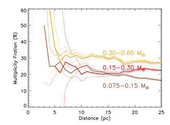
Figure 19: Cumulative stellar multiplicity rate by primary mass. Shown are the running multiplicity rates of the three mass subsets binned by one parsec, with the masses of the primaries calculated from deblended photometry: primary masses 0.30–0.60 M_⊙ (orange line), with an uncorrected multiplicity rate at 25 pc of 28.2$\pm$2.1%; primary masses 0.15–0.30 M_⊙ (red line) with an uncorrected multiplicity rate at 25 pc of 21.4$\pm$2.0%; and primary masses 0.075–0.15 M_⊙ (brown line), with an uncorrected multiplicity rate at 25 pc of 16.0$\pm$2.5%. The dashed orange line indicates the addition of the 28 systems that have a primary mass larger than 0.60 M_⊙. The dotted lines on each curve indicate the Poisson errors. The large scatter and errors on the curves at distances less than 10 pc are due to small number of statistics. Neither suspected nor substellar companions are included. The largest mass bin has a higher multiplicity rate than the two smaller mass bins. It appears likely that multiple systems are missing from the smallest mass bin at distances 18 to 25 pc, as the curve decreases at those distances.

Figure 19 illustrates the multiplicity rate dependence for three mass regimes subdivided into mass bins that span factors of two — 0.30–0.60 M_⊙, 0.15–0.30 M_⊙, and 0.075–0.15 M_⊙ — as a function of distance for the target stars. No corrections have been applied for undetected companions in any of the three subsamples. The dashed orange line shows the contribution of the 28 systems that have a primary mass larger than 0.60 M_⊙, of which ten are multiple. It is evident that the highest mass bin of stars has the largest multiplicity rate at 15 pc (31.1$\pm$3.4%), roughly 10% greater than for lower masses (19.4$\pm$2.8% and 19.8$\pm$3.6% for the mid- and low-mass bins, respectively) at the same distance horizon. These values are consistent with Figure 3 in Janson et al. (2012) and Figure 7 in Janson et al. (2014a), although their sample only extends to spectral type M6, so they do not address our lowest mass bin. It also appears that there are slight dropoffs in detected multiples for the highest and lowest mass bins from 15 to 25 pc, whereas the multiplicity rate for the medium-mass bin remains fairly flat. The dropoff for the highest mass stars is only 2%, a shift that we deem insignificant. However, the dropoff for the lowest mass stars is 4% from 15 to 25 pc and in fact is 9% from 11 to 25 pc. This is likely because the lowest mass primaries are the most difficult to study, so some companions have yet to be detected. Nonetheless, the overall situation is clear: high-mass M dwarfs have more stellar companions than low-mass M dwarfs.

Figure 20: Mass ratios and log-separation distributions for subsamples of M dwarfs as a function of primary masses. Mass ratios for primaries with masses 0.30–0.60 M_⊙ (in orange, top left) with the ten multiple systems with primaries more massive than 0.60 M_⊙ shown unfilled; for primaries with masses 0.15–0.30 M_⊙ (in red, top middle); mass ratios for primaries with masses 0.075–0.15 M_⊙ (in brown, top right). The mass ratio ranges shrink as a function of decreasing primary mass in part due to the imposed lower stellar companion mass limit of 0.075 M_⊙, although some effect due to gravitational binding energy is likely. Distribution of the projected separations for companions to stars with 0.30–0.60 M_⊙ (bottom left), with the ten multiple systems with primaries more massive than 0.60 M_⊙ shown unfilled; for companions to stars with 0.15–0.30 M_⊙ (bottom middle); for companions to stars with 0.075 $-$ 0.15 M_⊙ (bottom right). The axis scales are the same for both trio of plots to highlight the differences between each mass subsample. The peaks of the projected separation distributions shift to smaller separations with decreasing primary mass subset.

With our large sample, it is also possible to evaluate the mass ratio and separation distributions by mass subset. Figure 20 presents the mass ratios (top row of three plots) and the log of the projected separations in AU (bottom row of three plots, discussed below) of the 310 stellar components by mass subset.

It is evident that the number of multiples in each subset decreases with decreasing primary mass, as shown more explicitly in Figure 19. Of note is the wide range in the mass ratios for the most massive primaries, indicating that such stars tend to form with companions filling nearly the entire suite of possible masses. There is also a general shift to larger mass ratios with decreasing primary masses. This trend is somewhat expected because we have set a hard limit on companion masses by only including stellar companions, and there is a decreasing amount of mass phase space available as the primary’s mass approaches this stellar/sub-stellar boundary; as noted in §3.4.4, brown dwarf companions have been excluded from the analysis. Thus, it appears that lower mass red dwarfs may only form and/or gravitationally retain companions when they are of comparable mass and at small separations. We conclude that M dwarfs have nearly every type of lower mass companion star.

We next evaluate how the mass of the primary drives the separations at which companions are found. The bottom three panels of Figure 20 show the log-projected separation distributions for the three mass subsets. Again, the axis scales are the same between plots, and no substellar or suspected companions are included in these histograms. As in the top row of plots, the number of multiples decreases as a function of primary mass. It is evident that the distribution peaks move to smaller separations as a function of decreasing primary mass, following the trend from solar-type stars to M dwarfs as a whole. Comparison of our distribution peak for the mid-mass sub-sample, which corresponds most closely to the mid-M sample surveyed in Janson et al. (2014a), shows a peak within the range of the projected separations (11 AU) of the peak reported from their survey (3–10 AU).

6.2 Understanding How Tangential Velocity Influences the Multiplicity Rate and Companion Separations

Figure 21: Histogram of primary tangential velocity. The tangential velocity of the primary (or single) component in each system is plotted in gray, with the primaries of confirmed multiple systems indicated in blue. Overplotted in red is the curve of the running multiplicity rate as a function of $v_{tan}$, indicating that slower moving objects tend to have companions slightly more often. Poisson errors on the multiplicity fraction are indicated by dotted lines.

Because it is known that the tangential velocity, $v_{tan}$, of a star generally increases with age due to gravitational kicks from objects in the Milky Way (usually from Giant Molecular Clouds), cool subdwarfs will generally have larger velocities (e.g., $v_{tan}$ $>$ 200 km s^-1; Jao et al., 2017) than young stars (estimated to be $v_{tan}$ $<$ 35 km s^-1). Thus, we investigate M dwarf multiplicity as a function of $v_{tan}$, which we use as a proxy for age. Figure 21 shows the $v_{tan}$ distribution of the observed sample, using the $v_{tan}$ of the primary component, where singles are shown in gray and multiples in blue. There are noticeably more multiple systems with $v_{tan}$ $<$ 50 km s^-1 than at larger $v_{tan}$. The overplotted red curve gives the running multiplicity rate as a function of $v_{tan}$, showing a general decrease in multiplicity with increasing $v_{tan}$. The apparent drop in the MR at $v_{tan}$ $\approx$ 15 km s^-1 is due to the incompleteness of the sample at low proper motions and corresponding $v_{tan}$ values, and is not a real trend. This implies that as small stars age and experience kicks in their travels through the Galaxy, they lose companions. Alternately, these older stars may have experienced different multiplicity formation rates at the outset, either because of different (presumably lower) metallicities, or different star formation environments.

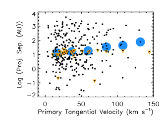
Figure 22: The log of the projected separation in AU as a function of tangential velocity for the 310 stellar pairs. Not shown is the one subdwarf binary with $v_{tan}$ $>$ 150 km s^-1. A weak trend of increasing projected separation with increasing tangential velocity is seen. This is emphasized by the large blue points indicating the log of the median projected linear separation as a function of the median tangential velocity, in bins of 25 km s^-1. Pairs with estimated upper limits on their separations have been indicated with inverted orange triangles.

Figure 22 further illustrates how multiplicity changes with $v_{tan}$, showing the log of the projected separation as a function of $v_{tan}$. The blue open circles represent the log of the median projected separation in 25 km s^-1 bins, illustrating a weak trend of increasing projected separation with increasing $v_{tan}$. The pairs for which the separations are upper limits are more numerous at the slower end of the plot, hinting that the median $v_{tan}$ may decrease even further there, once true separations are available for those close pairs. Thus, the overall trends are that faster moving stars have fewer companions, and that the separations of multiples with higher velocities tend to be larger than their slower-moving counterparts.

6.3 The Luminosity and Mass Distributions

Figure 23: Luminosity Distributions. (top) The luminosity distribution for the 1214 M dwarfs in the sample with individual photometry. $M_{V}$ has been calculated from the blended photometry. (bottom) The luminosity distribution for all 1432 M dwarf primaries and secondaries in the sample with $M_{V}$ calculated from deblended photometry. Primaries are plotted in red; companions in blue. The vertical lines denote the subdivisions by factors of two in mass explored throughout the study. The contributions from the companions in the deblended luminosity distribution are greater than in the blended luminosity distribution.

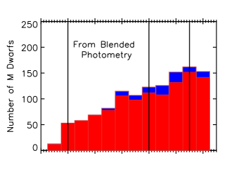
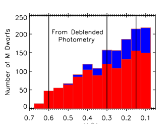
Figure 24: Mass Distributions. (top) The mass distribution for the 1214 M dwarfs in the sample with masses estimated from blended photometry. (bottom) The mass distribution for all 1432 M dwarfs in the sample with masses estimated from deblended photometry. Primaries are plotted in red; stellar companions in blue. The vertical lines denote the subdivisions by factors of two in mass explored throughout the study. There is a noticeable difference in the shapes of the distributions, as the contributions from the low mass companions contribute to the rise of the mass distribution to the end of the main sequence.

Shown in Figure 23 are luminosity distributions for our sample in $M_{V}$, calculated both before (top) and after (bottom) deblending ‘joint’ photometry with contributions from close companions. Primaries are indicated in red, while companions are shown in blue. The vertical lines at $M_{V}$ $=$ 9.25, 11.80, and 13.86 correspond to masses of 0.60, 0.30, and 0.15 M_⊙ and indicate the factors of two in mass used to further divide the 25 pc sample for the analysis presented in 6.1. It is evident that a substantial number of companions were hiding in the blended photometry of the M dwarf primaries.

Figure 24 illustrates the mass distribution for the 1214 M dwarfs with individual photometry with masses calculated from blended photometry (top) and the distribution for all 1432 M dwarf components (primaries plus all secondaries) found within 25 pc in the survey after deblending photometry (bottom). Both histograms show a gentle, but steady rise to the end of the stellar main sequence, what we have defined to be 0.075 M_⊙. This trend is emphasized by the additions of the companions in each histogram, as they are all lower masses than their primaries, by definition. Given that there are missing M dwarf systems within 25 pc that are preferentially of low mass, the mass distribution will ultimately be even steeper than shown.

6.3.1 Mass Contributions from Primaries and Hidden Companions

We now consider the contributions to the Galactic mass budget by M dwarfs. Without any prior knowledge of unresolved companions, a naive estimate of the mass of the 1214 M dwarfs in the sample with indivdually measured photometry, from which masses are estimated, yields 381 M_⊙. This includes the 1120 M dwarf primaries plus their 94 well-separated secondaries.

However, of the 265 primaries in the sample of multiples, 210 have 257 companions located at angular separations of less than 2″ from either their primaries or their widely separated secondaries, resulting in ‘joint’, or blended, $V$ magnitudes. After deblending, we find that the 1120 primaries contribute 336 M_⊙. The deblended companions have added 45 $M_{\odot}$ to the total M dwarf mass, indicating that 11% was hidden as unresolved stars. We find that at least 17% (66 M_⊙/402 M_⊙) of M dwarf mass is found in companions, with unresolved companions contributing at least 68% (45 M_⊙/66 M_⊙) of the companion mass and donating 11% (45 M_⊙/402 M_⊙) to the total mass budget of M dwarfs. We emphasize that these values are all lower limits, as this collection of M dwarfs has not been thoroughly canvassed for companions at separations of less than 2″, where most M dwarf companions are found.

6.4 Comparisons to Previous Work on Other Stellar Populations

We now put the results from this survey in perspective by making comparisons to results from other M dwarf multiplicity surveys, as well as to surveys of more massive stars. We then discuss how unresolved companions affect the red dwarf luminosity and mass distributions. Finally, directions for future work will be outlined.

6.4.1 Comparison to Other M Dwarf Surveys

As noted in §1, previous surveys have been done to determine M dwarf multiplicity, but most have studied samples on the order of a hundred stars. Some of the surveys (Skrutskie et al., 1989; Delfosse et al., 1999a) did not report a multiplicity rate in their results, so they will not be addressed. Others explored the regions around M dwarfs in search of different types of objects (brown dwarfs in the case of Dieterich et al. (2012) and Jovian mass planets in the case of Endl et al. (2006)) or at different separation regimes (Dhital et al. (2010) and Law et al. (2010) explored only the wide binary rate) and are thus not relevant to the present comparison. For example, searches for substellar objects can provide lower limits for the types of companions found around M dwarfs, but stellar companions are not always reported. Law et al. (2006, 2008) probed different sample sizes of late-type M dwarfs using lucky imaging and report multiplicity rates that are different from each other by a factor of two, but still within their large errors. We note that the uncorrected multiplicity rate calculated here for the lowest mass bin of M dwarfs — 16.0$\pm$2.5% — agrees with that reported in Law et al. (2008): 13.6 ${}^{+6.5}_{-4}$%.

A number of the other samples studied for M dwarf multiplicity determination were volume-limited. Henry & McCarthy (1990) searched the 5 pc sample of M dwarfs, while Henry (1991) and Simons et al. (1996) extended the volume searched to 8 pc. Fischer & Marcy (1992) searched a varied sample of M dwarfs within 20 pc. The samples of Bergfors et al. (2010), Janson et al. (2012), and Janson et al. (2014a) were all within 52 pc, but most distances were photometric parallaxes.

We find that our multiplicity rate result agrees with most of the more recent surveys. Bergfors et al. (2010), Janson et al. (2012), and Janson et al. (2014a) report MRs of 32%, 27%, and 21–27%, respectively. Our results also agree with the earlier studies of Henry & McCarthy (1990) and Henry (1991) (34% and 20%) within the errors, but are smaller than the studies of Fischer & Marcy (1992) and Simons et al. (1996) (42% and 40%). It is likely that some of the earlier studies simply did not have enough targets from which to calculate accurate results with low statistical errors.

The only other sizeable survey that was volume-limited and had trigonometric parallaxes available was that of Ward-Duong et al. (2015); however, their sample included late K dwarfs and did not include any late M dwarfs. We find a slightly larger multiplicity rate than the 23.5$\pm$3.2% of Ward-Duong et al. (2015), although results agree within the errors. Examination of the sample studied here reveals an additional 308 M dwarfs with parallaxes from sources other than van Leeuwen (2007) that place them within 15 pc, 247 of which are within the color-limits of their sample (3.65 $<$ $(V-K)$ $\lesssim$ 6.8).

Due to all of the targets in our multiplicity sample having accurate trigonometric parallaxes, the study presented here has a number of advantages over ones conducted by others. All of the targets considered were reliably known to be within 25 pc. Because we measured $VRI$ photometry for almost all targets lacking it, we were able to use a homogeneous set of data on the same photometric system, combined with the existing parallaxes, to calculate $M_{V}$ and thus, estimate masses. Most other surveys were forced to use less accurate types of distances to draw conclusions from their data. We were also able to calculate projected separations that were more accurate than those of others, as our sample has trigonometric distances. Finally, our survey was comprehensive in two search regimes, while also able to infer the presence of candidate companions using other methods.

6.4.2 Comparison to More Massive Stars

Listed in Table 6.4.2 are the multiplicity statistics for stars of other main sequence spectral types, along with the percentages of all stars by that spectral type. While brown dwarfs are not main sequence objects, they have been included for comparison. The percentage of stars that they comprise has been purposely left blank, as they are not stars, and in fact, the size of the brown dwarf population is not well constrained.

While the multiplicity rate decreases as a function of primary mass, it is evident that the number of stars increases with decreasing mass. Massive stars of types OBA are the most rare, accounting for fewer than 1% of all stars (Binney & Merrifield, 1998), while solar-type FGK stars make up $\sim$21% of all stars (Binney & Merrifield, 1998). The M dwarfs make up 75% of all stars; thus, their multiplicity statistics have the largest impact. The K dwarf multiplicity rate is the most uncertain, with no comprehensive multiplicity search having yet been done for that spectral type, although efforts to remedy this are currently underway by members of the RECONS group. The thorough study presented here provides an anchor for the statistics at the low end of the stellar main sequence, enabling a complete picture of stellar multiplicity.

Table 15: Multiplicity of Main Sequence Stars

Spectral	% of	Ref	Mult.	Comp	Ref
Type	Stars		Rate	Rate
O	$<$0.1	2	$>$80	130	5,3
B	0.1	2	$>$70	100	6,3
A	0.6	2	$>$70	100	6,3
F	3.3	2	50$\pm$4	75	6
G	7.8	2	46$\pm$2	75	6
K	10.2	2	41$\pm$3	56	6
M	75.0	4	26.8$\pm$1.4	32.4$\pm$1.4	1
L,T	$\cdots$		22	22	3

Note. — The columns indicate the spectral type of object, the percentage of stars that each spectral type comprises, along with the reference. Next, the Multiplicity Rate, the Companion Rate and the reference are listed.

References. — (1) this work; (2) Binney & Merrifield (1998); (3) Duchêne & Kraus (2013); (4) Henry et al. (2006); (5) Mason et al. (2009); (6) Raghavan et al. (2010).

Figure 25: Multiplicity rate as a function of spectral type. Shown is the MR for dwarf stars, with the rates for M dwarfs presented here in red. Open red points are the uncorrected MRs for the three mass bins explored throughout this paper, while the solid point is the total corrected MR for all M dwarfs. Values for stars more massive than M dwarfs are taken from the literature, as listed in Table 6.4.2. The open green and orange points are the blue and red subsamples from Raghavan et al. (2010), while the solid yellow point is the average reported in that paper. The arrows indicate the MRs that are likely lower limits. We do not include the L dwarfs here. Clearly, the MR is a function of decreasing mass.

Figure 25 indicates the multiplicity rates for dwarf stars, with values taken from the literature for the more massive main sequence stars. The clear decrease in multiplicity with decreasing primary mass is evident.

From this comprehensive picture of stellar multiplicity, we can determine the multiplicity rate of all star systems. Consider one million stars. Table 16 duplicates the percentages of stars for each main sequence spectral type and the multiplicity rate for each of those spectral types from Table 6.4.2. In addition, however, is listed the number of stars per one million that each spectral type would contribute and how many of those would be multiple. The extra three percent of stars not shown in the second column are made up of giants, supergiants, and white dwarfs (Binney & Merrifield, 1998). Based on the numbers presented, we can conclude that the multiplicity rate of all main sequence star systems is 31$\pm$0.05%, and that therefore, most stellar systems are single.

Table 16: Multiplicity Example

Spectral	% of	# of	Mult.	# Mult.
Type	Stars	Stars	Rate
O	0.003	30	80	24
B	0.1	1,000	70	700
A	0.6	6,000	70	4,200
F	3.3	33,000	50	16,500
G	7.8	78,000	46	35,880
K	10.2	102,000	41	41,820
M	75.0	750,000	26.8	201,000
	97.0	970,030	31	300,124

7 Conclusions

7.1 Summary of Results

$\bullet$ We report 20 new and 56 suspected companions to M dwarfs within 25 pc;

$\bullet$ We find a corrected multiplicity rate of 26.8$\pm$1.4% and a corrected companion rate of 32.4$\pm$1.4% for M dwarfs;

$\bullet$ We find that M dwarfs have multiplicity and companion rates of 20.2$\pm$1.2% and 23.9$\pm$1.4% at projected linear separations $<$ 50 AU;

$\bullet$ We find the uncorrected multiplicity rate of the three mass subsets (0.30 — 0.60 M/M_⊙, 0.15 — 0.30 M/M_⊙, and 0.075 — 0.15 M/M_⊙) to be 28.2$\pm$2.1%, 21.4$\pm$2.0%, and 16.0$\pm$2.5%;

$\bullet$ We find a uniformity in the mass ratio distribution, with no apparent preference in companion mass for the nearby M dwarfs;

$\bullet$ The distribution of the projected separations of the companions peaks at 4 – 20 AU for M dwarfs, i.e., the scale of the gas giants in our Solar System;

$\bullet$ A weak trend of decreasing projected separation with primary mass was found;

$\bullet$ A possible relation between multiplicity and tangential velocity was found, indicating that older, faster moving M dwarfs tend to have fewer companions at smaller separations as a population than their younger counterparts;

$\bullet$ We find that at least 17% of M dwarf mass is contained in companions, with 11% of the total mass budget made up of ‘hidden’ stellar companions;

$\bullet$ Finally, we demonstrate that the mass distribution of our volume-limited sample rises to the end of the stellar main sequence.

7.2 What Is Yet to Come

While the multiplicity survey presented here was comprehensive for stellar companions to M dwarfs with separations 2 – 300″, much work remains to be done. Currently underway are high-resolution speckle imaging and radial velocity studies to probe within 2″ of these nearby M dwarfs in order to complete our understanding of M dwarf multiplicity at all separation regimes. The results from these ongoing surveys will provide the separation and delta-magnitude measurements needed for a more thorough understanding of the characteristics of these multiple systems, e.g., the mass ratio and separation distributions. In addition, the radial velocities being measured provide the third velocity component needed to calculate precise $UVW$ space motions. These space motions will allow further exploration of the possible trend of stellar multiplicity with tangential velocity.

Gaia will have five years or more of exquisite astrometric measurements that will enable the detection of binaries. Any astrometric binary orbits should provide inclinations, and thus the dynamical masses of each component when combined with ground-based spectroscopic orbits. In addition, Gaia should reveal many of the very low-mass stars that have escaped detection to-date, providing a more complete picture of the nearby M dwarf population that we will study in the future.

8 Acknowledgments

We thank the anonymous referee for a rigorous review that greatly improved the manuscript. JGW is especially grateful to Jonathan Irwin, Willie Torres, and Eric Mamajek for illuminating and clarifying discussions and suggestions, and to Douglas Gies, Harold McAlister, Russel White, Sebastièn Lèpine and David Charbonneau for constructive comments. We thank Brian Mason for access to the Washington Double Star Catalog, a copy of which is housed at Georgia State University. JGW extends a heartfelt thanks to David Fanning for the availability of his IDL Coyote Graphics System.

We thank the members of the SMARTS Consortium, who have enabled the operations of the small telescopes at CTIO since 2003, as well as observers and observer support at CTIO, specifically Arturo Gomez, Mauricio Rojas, Hernan Tirado, Joselino Vasquez, Alberto Miranda, and Edgardo Cosgrove. We are indebted to the support staff and astronomers at Lowell Observatory for their assistance, particularly Len Bright, Larry Wasserman, Brian Skiff, and Ted Dunham.

Data products from the Two Micron All Sky Survey, which is a joint project of the University of Massachusetts and the Infrared Processing and Analysis Center/California Institute of Technology, funded by the National Aeronautics and Space Administration (NASA) and the NSF have been used extensively, as have the SIMBAD database and the Aladin and Vizier interfaces, operated at CDS, Strasbourg, France. This work has made ample use of the Smithsonian Astrophysical Observatory/NASA Astrophysics Data System. This work has made use of data from the European Space Agency (ESA) mission Gaia (https://www.cosmos.esa.int/gaia), processed by the Gaia Data Processing and Analysis Consortium (DPAC, https://www.cosmos.esa.int/web/gaia/dpac/consortium). Funding for the DPAC has been provided by national institutions, in particular the institutions participating in the Gaia Multilateral Agreement.

This work was made possible by National Science Foundation (NSF) grants 09-08402, 0507711, 1109445, and 141206, Sigma Xi Grants-In-Aid-of-Research, the generous budget allotment of Georgia State University that made possible access to the SMARTS telescopes at CTIO and Lowell, and the Georgia State University Dissertation grant. JGW was supported by a grant from the John Templeton Foundation for a portion of the time that it took to finalize these results. The opinions expressed here are those of the authors and do not necessarily reflect the views of the John Templeton Foundation.

References

- Al-Shukri et al. (1996) Al-Shukri, A. M., McAlister, H. A., Hartkopf, W. I., Hutter, D. J., & Franz, O. G. 1996, AJ, 111, 393
- Allen et al. (2007) Allen, P. R., Koerner, D. W., McElwain, M. W., Cruz, K. L., & Reid, I. N. 2007, AJ, 133, 971
- Allen & Reid (2008) Allen, P. R., & Reid, I. N. 2008, AJ, 135, 2024
- Andrei et al. (2011) Andrei, A. H., Smart, R. L., Penna, J. L., et al. 2011, AJ, 141, 54
- Anglada-Escudé et al. (2012) Anglada-Escudé, G., Boss, A. P., Weinberger, A. J., et al. 2012, ApJ, 746, 37
- Balega et al. (2013) Balega, I. I., Balega, Y. Y., Gasanova, L. T., et al. 2013, Astrophysical Bulletin, 68, 53
- Balega et al. (2007) Balega, I. I., Balega, Y. Y., Maksimov, A. F., et al. 2007, Astrophysical Bulletin, 62, 339
- Barbieri et al. (1996) Barbieri, C., De Marchi, G., Nota, A., et al. 1996, A&A, 315, 418
- Bartlett et al. (2017) Bartlett, J. L., Lurie, J. C., Riedel, A., et al. 2017, AJ, 154, 151
- Benedict et al. (2000) Benedict, G. F., McArthur, B. E., Franz, O. G., Wasserman, L. H., & Henry, T. J. 2000, AJ, 120, 1106
- Benedict et al. (1999) Benedict, G. F., McArthur, B., Chappell, D. W., et al. 1999, AJ, 118, 1086
- Benedict et al. (2001) Benedict, G. F., McArthur, B. E., Franz, O. G., et al. 2001, AJ, 121, 1607
- Benedict et al. (2002) Benedict, G. F., McArthur, B. E., Forveille, T., et al. 2002, ApJ, 581, L115
- Benedict et al. (2016) Benedict, G. F., Henry, T. J., Franz, O. G., et al. 2016, AJ, 152, 141
- Bergfors et al. (2010) Bergfors, C., Brandner, W., Janson, M., et al. 2010, A&A, 520, A54
- Bertin (2011) Bertin, E. 2011, in Astronomical Society of the Pacific Conference Series, Vol. 442, Astronomical Data Analysis Software and Systems XX, ed. I. N. Evans, A. Accomazzi, D. J. Mink, & A. H. Rots, 435
- Bertin & Arnouts (1996) Bertin, E., & Arnouts, S. 1996, A&AS, 117, 393
- Bessel (1990) Bessel, M. S. 1990, A&AS, 83, 357
- Bessell (1991) Bessell, M. S. 1991, AJ, 101, 662
- Bessell & Weis (1987) Bessell, M. S., & Weis, E. W. 1987, PASP, 99, 642
- Beuzit et al. (2004) Beuzit, J.-L., Ségransan, D., Forveille, T., et al. 2004, A&A, 425, 997
- Bidelman (1985) Bidelman, W. P. 1985, ApJS, 59, 197
- Biller & Close (2007) Biller, B. A., & Close, L. M. 2007, ApJ, 669, L41
- Biller et al. (2006) Biller, B. A., Kasper, M., Close, L. M., Brandner, W., & Kellner, S. 2006, ApJ, 641, L141
- Binney & Merrifield (1998) Binney, J., & Merrifield, M. 1998, Galactic Astronomy (Princeton University Press)
- Blake et al. (2008) Blake, C. H., Charbonneau, D., White, R. J., et al. 2008, ApJ, 678, L125
- Bonfils et al. (2013) Bonfils, X., Delfosse, X., Udry, S., et al. 2013, A&A, 549, A109
- Bonnefoy et al. (2009) Bonnefoy, M., Chauvin, G., Dumas, C., et al. 2009, A&A, 506, 799
- Bowler et al. (2015) Bowler, B. P., Liu, M. C., Shkolnik, E. L., & Tamura, M. 2015, ApJS, 216, 7
- Burningham et al. (2009) Burningham, B., Pinfield, D. J., Leggett, S. K., et al. 2009, MNRAS, 395, 1237
- Chanamé & Gould (2004) Chanamé, J., & Gould, A. 2004, ApJ, 601, 289
- Cortes-Contreras et al. (2014) Cortes-Contreras, M., Caballero, J. A., & Montes, D. 2014, The Observatory, 134, 348
- Costa et al. (2005) Costa, E., Méndez, R. A., Jao, W.-C., et al. 2005, AJ, 130, 337
- Costa et al. (2006) —. 2006, AJ, 132, 1234
- Cvetković et al. (2015) Cvetković, Z., Pavlović, R., & Boeva, S. 2015, AJ, 149, 150
- Daemgen et al. (2007) Daemgen, S., Siegler, N., Reid, I. N., & Close, L. M. 2007, ApJ, 654, 558
- Dahn et al. (1988) Dahn, C. C., Harrington, R. S., Kallarakal, V. V., et al. 1988, AJ, 95, 237
- Dahn et al. (2002) Dahn, C. C., Harris, H. C., Vrba, F. J., et al. 2002, AJ, 124, 1170
- Davison et al. (2014) Davison, C. L., White, R. J., Jao, W.-C., et al. 2014, AJ, 147, 26
- Davison et al. (2015) Davison, C. L., White, R. J., Henry, T. J., et al. 2015, AJ, 149, 106
- Dawson & De Robertis (2005) Dawson, P. C., & De Robertis, M. M. 2005, PASP, 117, 1
- Deacon & Hambly (2001) Deacon, N. R., & Hambly, N. C. 2001, A&A, 380, 148
- Deacon et al. (2005a) Deacon, N. R., Hambly, N. C., & Cooke, J. A. 2005a, A&A, 435, 363
- Deacon et al. (2005b) Deacon, N. R., Hambly, N. C., Henry, T. J., et al. 2005b, AJ, 129, 409
- Delfosse et al. (1999a) Delfosse, X., Forveille, T., Beuzit, J.-L., et al. 1999a, A&A, 344, 897
- Delfosse et al. (1998) Delfosse, X., Forveille, T., Perrier, C., & Mayor, M. 1998, A&A, 331, 581
- Delfosse et al. (1999b) Delfosse, X., Forveille, T., Udry, S., et al. 1999b, A&A, 350, L39
- Dhital et al. (2010) Dhital, S., West, A. A., Stassun, K. G., & Bochanski, J. J. 2010, AJ, 139, 2566
- Díaz et al. (2007) Díaz, R. F., González, J. F., Cincunegui, C., & Mauas, P. J. D. 2007, A&A, 474, 345
- Dieterich et al. (2012) Dieterich, S. B., Henry, T. J., Golimowski, D. A., Krist, J. E., & Tanner, A. M. 2012, AJ, 144, 64
- Dieterich et al. (2014) Dieterich, S. B., Henry, T. J., Jao, W.-C., et al. 2014, AJ, 147, 94
- Docobo et al. (2006) Docobo, J. A., Tamazian, V. S., Balega, Y. Y., & Melikian, N. D. 2006, AJ, 132, 994
- Docobo et al. (2010) —. 2010, AJ, 140, 1078
- Doyle & Butler (1990) Doyle, J. G., & Butler, C. J. 1990, A&A, 235, 335
- Duchêne & Kraus (2013) Duchêne, G., & Kraus, A. 2013, ARA&A, 51, 269
- Dupuy & Liu (2012) Dupuy, T. J., & Liu, M. C. 2012, ApJS, 201, 19
- Duquennoy & Mayor (1988) Duquennoy, A., & Mayor, M. 1988, A&A, 200, 135
- Endl et al. (2006) Endl, M., Cochran, W. D., Kürster, M., et al. 2006, ApJ, 649, 436
- Fabricius & Makarov (2000) Fabricius, C., & Makarov, V. V. 2000, A&AS, 144, 45
- Faherty et al. (2012) Faherty, J. K., Burgasser, A. J., Walter, F. M., et al. 2012, ApJ, 752, 56
- Falin & Mignard (1999) Falin, J. L., & Mignard, F. 1999, A&AS, 135, 231
- Femenía et al. (2011) Femenía, B., Rebolo, R., Pérez-Prieto, J. A., et al. 2011, MNRAS, 413, 1524
- Fischer & Marcy (1992) Fischer, D. A., & Marcy, G. W. 1992, ApJ, 396, 178
- Forveille et al. (2005) Forveille, T., Beuzit, J.-L., Delorme, P., et al. 2005, A&A, 435, L5
- Frankowski et al. (2007) Frankowski, A., Jancart, S., & Jorissen, A. 2007, A&A, 464, 377
- Freed et al. (2003) Freed, M., Close, L. M., & Siegler, N. 2003, ApJ, 584, 453
- Fu et al. (1997) Fu, H.-H., Hartkopf, W. I., Mason, B. D., et al. 1997, AJ, 114, 1623
- Gaia Collaboration et al. (2018) Gaia Collaboration, Brown, A. G. A., Vallenari, A., et al. 2018, ArXiv e-prints, arXiv:1804.09365
- Gaia Collaboration et al. (2016) Gaia Collaboration, Prusti, T., de Bruijne, J. H. J., et al. 2016, A&A, 595, A1
- Gatewood (2008) Gatewood, G. 2008, AJ, 136, 452
- Gatewood & Coban (2009) Gatewood, G., & Coban, L. 2009, AJ, 137, 402
- Gatewood et al. (2003) Gatewood, G., Coban, L., & Han, I. 2003, AJ, 125, 1530
- Gatewood et al. (1993) Gatewood, G., de Jonge, K. J., & Stephenson, B. 1993, PASP, 105, 1101
- Gershberg et al. (1999) Gershberg, R. E., Katsova, M. M., Lovkaya, M. N., Terebizh, A. V., & Shakhovskaya, N. I. 1999, A&AS, 139, 555
- Gianninas et al. (2011) Gianninas, A., Bergeron, P., & Ruiz, M. T. 2011, ApJ, 743, 138
- Gizis (1997) Gizis, J. E. 1997, AJ, 113, 806
- Gizis (1998) —. 1998, AJ, 115, 2053
- Gizis et al. (2002) Gizis, J. E., Reid, I. N., & Hawley, S. L. 2002, AJ, 123, 3356
- Golimowski et al. (2004) Golimowski, D. A., Leggett, S. K., Marley, M. S., et al. 2004, AJ, 127, 3516
- Gould & Chanamé (2004) Gould, A., & Chanamé, J. 2004, ApJS, 150, 455
- Graham (1982) Graham, J. A. 1982, PASP, 94, 244
- Gray et al. (2003) Gray, R. O., Corbally, C. J., Garrison, R. F., McFadden, M. T., & Robinson, P. E. 2003, AJ, 126, 2048
- Harlow (1996) Harlow, J. J. B. 1996, AJ, 112, 2222
- Harrington & Dahn (1980) Harrington, R. S., & Dahn, C. C. 1980, AJ, 85, 454
- Harrington et al. (1985) Harrington, R. S., Kallarakal, V. V., Christy, J. W., et al. 1985, AJ, 90, 123
- Harrington et al. (1993) Harrington, R. S., Dahn, C. C., Kallarakal, V. V., et al. 1993, AJ, 105, 1571
- Hartkopf et al. (2012) Hartkopf, W. I., Tokovinin, A., & Mason, B. D. 2012, AJ, 143, 42
- Hawley et al. (1996) Hawley, S. L., Gizis, J. E., & Reid, I. N. 1996, AJ, 112, 2799
- Heintz (1976) Heintz, W. D. 1976, MNRAS, 175, 533
- Heintz (1985) —. 1985, ApJS, 58, 439
- Heintz (1986) —. 1986, AJ, 92, 446
- Heintz (1987) —. 1987, ApJS, 65, 161
- Heintz (1990) —. 1990, ApJS, 74, 275
- Heintz (1991) —. 1991, AJ, 101, 1071
- Heintz (1992) —. 1992, ApJS, 83, 351
- Heintz (1993) —. 1993, AJ, 105, 1188
- Heintz (1994) —. 1994, AJ, 108, 2338
- Hełminiak et al. (2009) Hełminiak, K. G., Konacki, M., Kulkarni, S. R., & Eisner, J. 2009, MNRAS, 400, 406
- Henry (1991) Henry, T. J. 1991, PhD thesis, Arizona Univ., Tucson.
- Henry et al. (1999) Henry, T. J., Franz, O. G., Wasserman, L. H., et al. 1999, ApJ, 512, 864
- Henry et al. (1997) Henry, T. J., Ianna, P. A., Kirkpatrick, J. D., & Jahreiss, H. 1997, AJ, 114, 388
- Henry et al. (2006) Henry, T. J., Jao, W.-C., Subasavage, J. P., et al. 2006, AJ, 132, 2360
- Henry & McCarthy (1990) Henry, T. J., & McCarthy, Jr., D. W. 1990, ApJ, 350, 334
- Henry et al. (2004) Henry, T. J., Subasavage, J. P., Brown, M. A., et al. 2004, AJ, 128, 2460
- Henry et al. (2018) Henry, T. J., Jao, W.-C., Winters, J. G., et al. 2018, AJ, 155, 265
- Herbig & Moorhead (1965) Herbig, G. H., & Moorhead, J. M. 1965, ApJ, 141, 649
- Hershey & Taff (1998) Hershey, J. L., & Taff, L. G. 1998, AJ, 116, 1440
- Høg et al. (2000) Høg, E., Fabricius, C., Makarov, V. V., et al. 2000, A&A, 355, L27
- Holman & Wiegert (1999) Holman, M. J., & Wiegert, P. A. 1999, AJ, 117, 621
- Horch et al. (2012) Horch, E. P., Bahi, L. A. P., Gaulin, J. R., et al. 2012, AJ, 143, 10
- Horch et al. (2010) Horch, E. P., Falta, D., Anderson, L. M., et al. 2010, AJ, 139, 205
- Horch et al. (2011a) Horch, E. P., Gomez, S. C., Sherry, W. H., et al. 2011a, AJ, 141, 45
- Horch et al. (2002) Horch, E. P., Robinson, S. E., Meyer, R. D., et al. 2002, AJ, 123, 3442
- Horch et al. (2011b) Horch, E. P., van Altena, W. F., Howell, S. B., Sherry, W. H., & Ciardi, D. R. 2011b, The Astronomical Journal, 141, 180
- Horch et al. (2015a) Horch, E. P., van Belle, G. T., Davidson, Jr., J. W., et al. 2015a, AJ, 150, 151
- Horch et al. (2009) Horch, E. P., Veillette, D. R., Baena Gallé, R., et al. 2009, AJ, 137, 5057
- Horch et al. (2015b) Horch, E. P., van Altena, W. F., Demarque, P., et al. 2015b, AJ, 149, 151
- Horch et al. (2017) Horch, E. P., Casetti-Dinescu, D. I., Camarata, M. A., et al. 2017, AJ, 153, 212
- Hosey et al. (2015) Hosey, A. D., Henry, T. J., Jao, W.-C., et al. 2015, AJ, 150, 6
- Houdebine (2010) Houdebine, E. R. 2010, MNRAS, 407, 1657
- Howell (2000) Howell, S. B. 2000, Handbook of CCD Astronomy (Cambridge University Press)
- Howell (2012) —. 2012, PASP, 124, 263
- Ianna et al. (1996) Ianna, P. A., Patterson, R. J., & Swain, M. A. 1996, AJ, 111, 492
- Ireland et al. (2008) Ireland, M. J., Kraus, A., Martinache, F., Lloyd, J. P., & Tuthill, P. G. 2008, ApJ, 678, 463
- Jahreiß et al. (2008) Jahreiß, H., Meusinger, H., Scholz, R.-D., & Stecklum, B. 2008, A&A, 484, 575
- Jancart et al. (2005) Jancart, S., Jorissen, A., Babusiaux, C., & Pourbaix, D. 2005, A&A, 442, 365
- Janson et al. (2014a) Janson, M., Bergfors, C., Brandner, W., et al. 2014a, ApJ, 789, 102
- Janson et al. (2012) Janson, M., Hormuth, F., Bergfors, C., et al. 2012, ApJ, 754, 44
- Janson et al. (2014b) Janson, M., Bergfors, C., Brandner, W., et al. 2014b, ApJS, 214, 17
- Jao et al. (2008) Jao, W.-C., Henry, T. J., Beaulieu, T. D., & Subasavage, J. P. 2008, AJ, 136, 840
- Jao et al. (2003) Jao, W.-C., Henry, T. J., Subasavage, J. P., et al. 2003, AJ, 125, 332
- Jao et al. (2005) —. 2005, AJ, 129, 1954
- Jao et al. (2014) —. 2014, AJ, 147, 21
- Jao et al. (2011) —. 2011, AJ, 141, 117
- Jao et al. (2017) Jao, W.-C., Henry, T. J., Winters, J. G., et al. 2017, AJ, 154, 191
- Jao et al. (2009) Jao, W.-C., Mason, B. D., Hartkopf, W. I., Henry, T. J., & Ramos, S. N. 2009, AJ, 137, 3800
- Jenkins et al. (2009) Jenkins, J. S., Ramsey, L. W., Jones, H. R. A., et al. 2009, ApJ, 704, 975
- Jódar et al. (2013) Jódar, E., Pérez-Garrido, A., Díaz-Sánchez, A., et al. 2013, MNRAS, 429, 859
- Khovritchev et al. (2013) Khovritchev, M. Y., Izmailov, I. S., & Khrutskaya, E. V. 2013, MNRAS, 435, 1083
- Kirkpatrick & McCarthy (1994) Kirkpatrick, J. D., & McCarthy, Jr., D. W. 1994, AJ, 107, 333
- Kleinman et al. (2004) Kleinman, S. J., Harris, H. C., Eisenstein, D. J., et al. 2004, ApJ, 607, 426
- Koen et al. (2002) Koen, C., Kilkenny, D., van Wyk, F., Cooper, D., & Marang, F. 2002, MNRAS, 334, 20
- Koen et al. (2010) Koen, C., Kilkenny, D., van Wyk, F., & Marang, F. 2010, MNRAS, 403, 1949
- Köhler et al. (2012) Köhler, R., Ratzka, T., & Leinert, C. 2012, A&A, 541, A29
- Kraus et al. (2016) Kraus, A. L., Ireland, M. J., Huber, D., Mann, A. W., & Dupuy, T. J. 2016, AJ, 152, 8
- Kürster et al. (2008) Kürster, M., Endl, M., & Reffert, S. 2008, A&A, 483, 869
- Kürster et al. (2009) Kürster, M., Zechmeister, M., Endl, M., & Meyer, E. 2009, The Messenger, 136, 39
- Lampens et al. (2007) Lampens, P., Strigachev, A., & Duval, D. 2007, A&A, 464, 641
- Landolt (1992) Landolt, A. U. 1992, AJ, 104, 372
- Landolt (2007) —. 2007, AJ, 133, 2502
- Landolt (2009) —. 2009, AJ, 137, 4186
- Landolt (2013) —. 2013, AJ, 146, 131
- Law et al. (2010) Law, N. M., Dhital, S., Kraus, A., Stassun, K. G., & West, A. A. 2010, ApJ, 720, 1727
- Law et al. (2006) Law, N. M., Hodgkin, S. T., & Mackay, C. D. 2006, MNRAS, 368, 1917
- Law et al. (2008) —. 2008, MNRAS, 384, 150
- Leinert et al. (1997) Leinert, C., Henry, T., Glindemann, A., & McCarthy, Jr., D. W. 1997, A&A, 325, 159
- Leinert et al. (1994) Leinert, C., Weitzel, N., Richichi, A., Eckart, A., & Tacconi-Garman, L. E. 1994, A&A, 291, L47
- Lèpine & Shara (2005) Lèpine, S., & Shara, M. M. 2005, AJ, 129, 1483
- Lèpine et al. (2009) Lèpine, S., Thorstensen, J. R., Shara, M. M., & Rich, R. M. 2009, AJ, 137, 4109
- Lindegren et al. (1997) Lindegren, L., Mignard, F., Söderhjelm, S., et al. 1997, A&A, 323, L53
- Lurie et al. (2014) Lurie, J. C., Henry, T. J., Jao, W.-C., et al. 2014, AJ, 148, 91
- Luyten (1979a) Luyten, W. J. 1979a, LHS Catalogue. Second edition. (University of Minnesota)
- Luyten (1979b) —. 1979b, NLTT catalogue. Volume_I. +90__to_+30_. Volume._II. +30__to_0_. (University of Minnesota)
- Luyten (1980a) —. 1980a, NLTT Catalogue. Volume_III. 0__to -30_. (University of Minnesota)
- Luyten (1980b) —. 1980b, NLTT Catalogue. Volume_IV. -30__to_-90_. (University of Minnesota)
- Malo et al. (2014) Malo, L., Artigau, É., Doyon, R., et al. 2014, ApJ, 788, 81
- Mamajek (2016) Mamajek, E. E. 2016, in IAU Symposium, Vol. 314, Young Stars & Planets Near the Sun, ed. J. H. Kastner, B. Stelzer, & S. A. Metchev, 21–26
- Mamajek et al. (2013) Mamajek, E. E., Bartlett, J. L., Seifahrt, A., et al. 2013, AJ, 146, 154
- Marcy & Benitz (1989) Marcy, G. W., & Benitz, K. J. 1989, ApJ, 344, 441
- Marcy et al. (1987) Marcy, G. W., Lindsay, V., & Wilson, K. 1987, PASP, 99, 490
- Martin & Mignard (1998) Martin, C., & Mignard, F. 1998, A&A, 330, 585
- Martín et al. (2000) Martín, E. L., Koresko, C. D., Kulkarni, S. R., Lane, B. F., & Wizinowich, P. L. 2000, ApJ, 529, L37
- Martinache et al. (2007) Martinache, F., Lloyd, J. P., Ireland, M. J., Yamada, R. S., & Tuthill, P. G. 2007, ApJ, 661, 496
- Martinache et al. (2009) Martinache, F., Rojas-Ayala, B., Ireland, M. J., Lloyd, J. P., & Tuthill, P. G. 2009, ApJ, 695, 1183
- Mason et al. (2009) Mason, B. D., Hartkopf, W. I., Gies, D. R., Henry, T. J., & Helsel, J. W. 2009, AJ, 137, 3358
- Mason et al. (2018) Mason, B. D., Hartkopf, W. I., Miles, K. N., et al. 2018, AJ, 155, 215
- McAlister et al. (1987) McAlister, H. A., Hartkopf, W. I., Hutter, D. J., & Franz, O. G. 1987, AJ, 93, 688
- McLean et al. (2003) McLean, I. S., McGovern, M. R., Burgasser, A. J., et al. 2003, ApJ, 596, 561
- Meyer et al. (2006) Meyer, R. D., Horch, E. P., Ninkov, Z., van Altena, W. F., & Rothkopf, C. A. 2006, PASP, 118, 162
- Monet et al. (2003) Monet, D. G., Levine, S. E., Canzian, B., et al. 2003, AJ, 125, 984
- Montagnier et al. (2006) Montagnier, G., Ségransan, D., Beuzit, J.-L., et al. 2006, A&A, 460, L19
- Montet et al. (2014) Montet, B. T., Crepp, J. R., Johnson, J. A., Howard, A. W., & Marcy, G. W. 2014, ApJ, 781, 28
- Morgan (1995) Morgan, D. H. 1995, in Astronomical Society of the Pacific Conference Series, Vol. 84, IAU Colloq. 148: The Future Utilisation of Schmidt Telescopes, ed. J. Chapman, R. Cannon, S. Harrison, & B. Hidayat, 137
- Nidever et al. (2002) Nidever, D. L., Marcy, G. W., Butler, R. P., Fischer, D. A., & Vogt, S. S. 2002, ApJS, 141, 503
- Perryman et al. (1997) Perryman, M. A. C., Lindegren, L., Kovalevsky, J., et al. 1997, A&A, 323, L49
- Platais et al. (2003) Platais, I., Pourbaix, D., Jorissen, A., et al. 2003, A&A, 397, 997
- Pokorny et al. (2004) Pokorny, R. S., Jones, H. R. A., Hambly, N. C., & Pinfield, D. J. 2004, A&A, 421, 763
- Pourbaix et al. (2003) Pourbaix, D., Platais, I., Detournay, S., et al. 2003, A&A, 399, 1167
- Pourbaix et al. (2004) Pourbaix, D., Tokovinin, A. A., Batten, A. H., et al. 2004, A&A, 424, 727
- Poveda et al. (1994) Poveda, A., Herrera, M. A., Allen, C., Cordero, G., & Lavalley, C. 1994, Rev. Mexicana Astron. Astrofis., 28, 43
- Pravdo & Shaklan (2009) Pravdo, S. H., & Shaklan, S. B. 2009, ApJ, 700, 623
- Pravdo et al. (2004) Pravdo, S. H., Shaklan, S. B., Henry, T., & Benedict, G. F. 2004, ApJ, 617, 1323
- Pravdo et al. (2006) Pravdo, S. H., Shaklan, S. B., Wiktorowicz, S. J., et al. 2006, ApJ, 649, 389
- Raghavan et al. (2010) Raghavan, D., McAlister, H. A., Henry, T. J., et al. 2010, ApJS, 190, 1
- Reid et al. (2001) Reid, I. N., Gizis, J. E., Kirkpatrick, J. D., & Koerner, D. W. 2001, AJ, 121, 489
- Reid et al. (1995) Reid, I. N., Hawley, S. L., & Gizis, J. E. 1995, AJ, 110, 1838
- Reid et al. (2002) Reid, I. N., Kilkenny, D., & Cruz, K. L. 2002, AJ, 123, 2822
- Reid et al. (2003) Reid, I. N., Cruz, K. L., Laurie, S. P., et al. 2003, AJ, 125, 354
- Reiners & Basri (2010) Reiners, A., & Basri, G. 2010, ApJ, 710, 924
- Reiners et al. (2012) Reiners, A., Joshi, N., & Goldman, B. 2012, AJ, 143, 93
- Riddle et al. (1971) Riddle, R. K., Priser, J. B., & Strand, K. A. 1971, Publications of the U.S. Naval Observatory Second Series, 20, 1
- Riedel et al. (2017) Riedel, A. R., Blunt, S. C., Lambrides, E. L., et al. 2017, AJ, 153, 95
- Riedel et al. (2011) Riedel, A. R., Murphy, S. J., Henry, T. J., et al. 2011, AJ, 142, 104
- Riedel et al. (2018) Riedel, A. R., Silverstein, M. L., Henry, T. J., et al. 2018, ArXiv e-prints, arXiv:1804.08812
- Riedel et al. (2010) Riedel, A. R., Subasavage, J. P., Finch, C. T., et al. 2010, AJ, 140, 897
- Riedel et al. (2014) Riedel, A. R., Finch, C. T., Henry, T. J., et al. 2014, AJ, 147, 85
- Salim & Gould (2003) Salim, S., & Gould, A. 2003, ApJ, 582, 1011
- Schilbach et al. (2009) Schilbach, E., Röser, S., & Scholz, R.-D. 2009, A&A, 493, L27
- Schmidt et al. (2007) Schmidt, S. J., Cruz, K. L., Bongiorno, B. J., Liebert, J., & Reid, I. N. 2007, AJ, 133, 2258
- Schneider et al. (2011) Schneider, A., Melis, C., Song, I., & Zuckerman, B. 2011, ApJ, 743, 109
- Scholz (2010) Scholz, R.-D. 2010, A&A, 515, A92
- Ségransan et al. (2000) Ségransan, D., Delfosse, X., Forveille, T., et al. 2000, A&A, 364, 665
- Shakht (1997) Shakht, N. A. 1997, Astronomical and Astrophysical Transactions, 13, 327
- Shkolnik et al. (2012) Shkolnik, E. L., Anglada-Escudé, G., Liu, M. C., et al. 2012, ApJ, 758, 56
- Shkolnik et al. (2010) Shkolnik, E. L., Hebb, L., Liu, M. C., Reid, I. N., & Collier Cameron, A. 2010, ApJ, 716, 1522
- Siegler et al. (2005) Siegler, N., Close, L. M., Cruz, K. L., Martín, E. L., & Reid, I. N. 2005, ApJ, 621, 1023
- Simons et al. (1996) Simons, D. A., Henry, T. J., & Kirkpatrick, J. D. 1996, AJ, 112, 2238
- Skrutskie et al. (1989) Skrutskie, M. F., Forrest, W. J., & Shure, M. 1989, AJ, 98, 1409
- Skrutskie et al. (2006) Skrutskie, M. F., Cutri, R. M., Stiening, R., et al. 2006, AJ, 131, 1163
- Smart et al. (2010) Smart, R. L., Ioannidis, G., Jones, H. R. A., Bucciarelli, B., & Lattanzi, M. G. 2010, A&A, 514, A84
- Smart et al. (2007) Smart, R. L., Lattanzi, M. G., Jahreiß, H., Bucciarelli, B., & Massone, G. 2007, A&A, 464, 787
- Snodgrass & Carry (2013) Snodgrass, C., & Carry, B. 2013, The Messenger, 152, 14
- Söderhjelm (1999) Söderhjelm, S. 1999, A&A, 341, 121
- Subasavage et al. (2005a) Subasavage, J. P., Henry, T. J., Hambly, N. C., Brown, M. A., & Jao, W.-C. 2005a, AJ, 129, 413
- Subasavage et al. (2005b) Subasavage, J. P., Henry, T. J., Hambly, N. C., et al. 2005b, AJ, 130, 1658
- Subasavage et al. (2009) Subasavage, J. P., Jao, W.-C., Henry, T. J., et al. 2009, AJ, 137, 4547
- Subasavage (2007) Subasavage, Jr., J. P. 2007, PhD thesis, Georgia State University
- Tamazian et al. (2006) Tamazian, V. S., Docobo, J. A., Melikian, N. D., & Karapetian, A. A. 2006, PASP, 118, 814
- Tanner et al. (2010) Tanner, A. M., Gelino, C. R., & Law, N. M. 2010, PASP, 122, 1195
- Teegarden et al. (2003) Teegarden, B. J., Pravdo, S. H., Hicks, M., et al. 2003, ApJ, 589, L51
- Teixeira et al. (2009) Teixeira, R., Ducourant, C., Chauvin, G., et al. 2009, A&A, 503, 281
- Tinney (1996) Tinney, C. G. 1996, MNRAS, 281, 644
- Tinney et al. (1995) Tinney, C. G., Reid, I. N., Gizis, J., & Mould, J. R. 1995, AJ, 110, 3014
- Tody (1986) Tody, D. 1986, in Proc. SPIE, Vol. 627, Instrumentation in astronomy VI, ed. D. L. Crawford, 733
- Tody (1993) Tody, D. 1993, in Astronomical Society of the Pacific Conference Series, Vol. 52, Astronomical Data Analysis Software and Systems II, ed. R. J. Hanisch, R. J. V. Brissenden, & J. Barnes, 173
- Tokovinin & Lépine (2012) Tokovinin, A., & Lépine, S. 2012, AJ, 144, 102
- Tokovinin (1992) Tokovinin, A. A. 1992, A&A, 256, 121
- van Altena et al. (1995) van Altena, W. F., Lee, J. T., & Hoffleit, D. 1995, VizieR Online Data Catalog, 1174, 0
- van Biesbroeck (1974) van Biesbroeck, G. 1974, ApJS, 28, 413
- van de Kamp (1975) van de Kamp, P. 1975, ARA&A, 13, 295
- van de Kamp & Worth (1972) van de Kamp, P., & Worth, M. D. 1972, AJ, 77, 762
- van Dessel & Sinachopoulos (1993) van Dessel, E., & Sinachopoulos, D. 1993, A&AS, 100, 517
- van Leeuwen (2007) van Leeuwen, F. 2007, A&A, 474, 653
- von Braun et al. (2011) von Braun, K., Boyajian, T. S., Kane, S. R., et al. 2011, ApJ, 729, L26
- Wahhaj et al. (2011) Wahhaj, Z., Liu, M. C., Biller, B. A., et al. 2011, ApJ, 729, 139
- Wang et al. (2014) Wang, J., Fischer, D. A., Xie, J.-W., & Ciardi, D. R. 2014, ApJ, 791, 111
- Ward-Duong et al. (2015) Ward-Duong, K., Patience, J., De Rosa, R. J., et al. 2015, MNRAS, 449, 2618
- Weis (1984) Weis, E. W. 1984, ApJS, 55, 289
- Weis (1986) —. 1986, AJ, 91, 626
- Weis (1987) —. 1987, AJ, 93, 451
- Weis (1988) —. 1988, Ap&SS, 142, 223
- Weis (1991a) —. 1991a, AJ, 102, 1795
- Weis (1991b) —. 1991b, AJ, 101, 1882
- Weis (1993) —. 1993, AJ, 105, 1962
- Weis (1994) —. 1994, AJ, 107, 1135
- Weis (1996) —. 1996, AJ, 112, 2300
- Weis (1999) —. 1999, AJ, 117, 3021
- Winn & Fabrycky (2015) Winn, J. N., & Fabrycky, D. C. 2015, ARA&A, 53, 409
- Winters et al. (2011) Winters, J. G., Henry, T. J., Jao, W.-C., et al. 2011, AJ, 141, 21
- Winters et al. (2015) Winters, J. G., Henry, T. J., Lurie, J. C., et al. 2015, AJ, 149, 5
- Winters et al. (2017) Winters, J. G., Sevrinsky, R. A., Jao, W.-C., et al. 2017, AJ, 153, 14
- Winters et al. (2018) Winters, J. G., Irwin, J., Newton, E. R., et al. 2018, AJ, 155, 125
- Woitas et al. (2003) Woitas, J., Tamazian, V. S., Docobo, J. A., & Leinert, C. 2003, A&A, 406, 293
- Worley (1961) Worley, C. E. 1961, PASP, 73, 167
- Worley (1962) —. 1962, AJ, 67, 396
- Worley & Mason (1998) Worley, C. E., & Mason, B. D. 1998, AJ, 116, 917
- Young et al. (1987) Young, A., Sadjadi, S., & Harlan, E. 1987, ApJ, 314, 272
- Zechmeister et al. (2009) Zechmeister, M., Kürster, M., & Endl, M. 2009, A&A, 505, 859