Physics-Constrained Deep Learning for High-dimensional Surrogate Modeling and Uncertainty Quantification without Labeled Data

Abstract

Surrogate modeling and uncertainty quantification tasks for PDE systems are most often considered as supervised learning problems where input and output data pairs are used for training. The construction of such emulators is by definition a small data problem which poses challenges to deep learning approaches that have been developed to operate in the big data regime. Even in cases where such models have been shown to have good predictive capability in high dimensions, they fail to address constraints in the data implied by the PDE model. This paper provides a methodology that incorporates the governing equations of the physical model in the loss/likelihood functions. The resulting physics-constrained, deep learning models are trained without any labeled data (e.g. employing only input data) and provide comparable predictive responses with data-driven models while obeying the constraints of the problem at hand. This work employs a convolutional encoder-decoder neural network approach as well as a conditional flow-based generative model for the solution of PDEs, surrogate model construction, and uncertainty quantification tasks. The methodology is posed as a minimization problem of the reverse Kullback-Leibler (KL) divergence between the model predictive density and the reference conditional density, where the later is defined as the Boltzmann-Gibbs distribution at a given inverse temperature with the underlying potential relating to the PDE system of interest. The generalization capability of these models to out-of-distribution input is considered. Quantification and interpretation of the predictive uncertainty is provided for a number of problems.

url]https://www.cics.nd.edu/ url]http://www.contmech.mw.tum.de/index.php?id=5 url]https://www.seas.upenn.edu/directory/profile.php?ID=237

1 Introduction

Surrogate modeling is computationally attractive for problems that require repetitive yet expensive simulations, such as determinsitsic design, uncertainty propagation, optimization under uncertainty or inverse modeling. Data-efficiency, uncertainty quantification and generalization are the main challenges facing surrogate modeling, especially for problems with high-dimensional stochastic input, such as material properties [bilionis2013multi], background potentials [charalampidis2018computing], etc.

Training surrogate models is commonly posed as a supervised learning problem, which requires simulation data as the target. Gaussian process (GP) models are widely used as emulators for physical systems [kennedy2000predicting] with built-in uncertainty quantification. The recent advances to scale GPs to high-dimensional input include Kronecker product decomposition that exploits the spatial structure [bilionis2013multi, wilson2015kernel, atkinson2018structured], convolutional kernels [NIPS2017_6877] and other algorithmic and software developments [gardner2018gpytorch]. However, GPs are still struggling to effectively model high-dimensional input-output maps. Deep neural networks (DNNs) are becoming the most popular surrogate models nowadays across engineering and scientific fields. As universal function approximators, DNNs excel at settings where both the input and output are high-dimensional. Applications in flow simulations include pressure projections in solving Navier-Stokes equations [doi:10.1002/cav.1695], fluid flow through random heterogeneous media [zhu2018bayesian, tripathy2018deep, mo2018deep], Reynolds-Averaged Navier-Stokes simulations [ling_kurzawski_templeton_2016, thuerey2018well, Geneva2019Quantifying] and others. Uncertainty quantification for DNNs is often studied under the re-emerging framework of Bayesian deep learning [doi:10.1162/neco.1992.4.3.448], mostly using variational inference for approximate posterior of model parameters, e.g. variational dropout [NIPS2015_5666, gal2016dropout], Stein variational gradient descent [NIPS2016_6338, zhu2018bayesian], although other methods exist, e.g. ensemble methods [lakshminarayanan2017simple]. Another perspective to high-dimensional problems is offered by latent variable models [2017arXiv171102475G], where the latent variables encode the information bottleneck between the input and output.

Sufficient amount of training data is usually required for the surrogates to achieve accurate predictions even under restricted settings, e.g. fixed boundary conditions. For physically-grounded domains, baking in the prior knowledge can potentially overcome the challenges of data-efficiency and generalization, etc. The inductive bias can be built into the network architecture, e.g. spherical convolutional neural networks (CNNs) for the physical fields on unstructured grid [jiang2018spherical], graph networks for object- and relation-centric representations of complex, dynamical systems [gn_icml18], learning linear embeddings of nonlinear dynamics based on Koopman operator theory [lusch2018deep]. Another approach is to embed physical laws into the learning systems, such as approximating differential operators with convolutions [pmlr-v80-long18a], enforcing hard constraint of mass conservation by learning the stream function [2018arXiv180602071K] whose curl is guaranteed to be divergence-free.

A more general way to incorporate physical knowledge is through constraint learning [2016arXiv160905566S], i.e. learning the models by minimizing the violation of the physical constraints, symmetries, e.g. cycle consistency in domain translation [CycleGAN2017], temporal coherence of consecutive frames in fluid simulation [xie2018tempogan] and video translation [wang2018vid2vid]. One typical example in computational physics is learning solutions of deterministic PDEs with neural networks in space/time, which dates back at least to the early $1990$s, e.g. [psichogios1992hybrid, meade1994numerical, lagaris1998artificial]. The main idea is to train neural networks to approximate the solution by minimizing the violation of the governing PDEs (e.g. the residual of the PDEs) and also of the initial and boundary conditions. In [lagaris1998artificial], a one-hidden-layer fully-connected neural network (FC-NN) with spatial coordinates as input is trained to minimize the residual norm evaluated on a fixed grid. The success of deep neural networks brings several new developments: (1) most of the works parameterize the solution with FC-NNs, thus the solution is analytical and meshfree [raissi2017physics, berg2018unified]; (2) the loss function can be derived from the variational form [weinan2018deep, nabian2018deep]; (3) stochastic gradient descent is used to train the network by randomly sampling mini-batches of inputs (spatial locations and/or time instances) [sirignano2018dgm, weinan2018deep]; (4) deeper networks are used to break the curse of dimensionality [grohs2018proof] allowing for several high-dimensional PDEs to be solved with high accuracy and speed [han2018solving, beck2017machine, sirignano2018dgm, raissi2018forward]; (5) multiscale numerical solvers are enhanced by replacing the linear basis with learned ones with DNNs [wang2018deep, fan2018multiscale]; (6) surrogate modeling for PDEs [CNNFluid2016, khoo2017solving, nabian2018deep].

Our work focuses on physics-constrained surrogate modeling for stochastic PDEs with high-dimensional spatially-varying coefficients without simulation data. We first show that when solving deterministic PDEs, the CNN-based parameterizations are more computationally efficient in capturing multiscale features of the solution fields than the FC-NN ones. Furthermore, we demonstrate that in comparison with image-to-image regression approaches that employ Deep NNs [zhu2018bayesian], the proposed method achieves comparable predictive performance, despite the fact that it does not make use of any output simulation data. In addition, it produces better predictions under extrapolative conditions as when out-of-distribution test input datasets are used. Finally, a flow-based conditional generative model is proposed to capture the predictive distribution with calibrated uncertainty, without compromising the predictive accuracy.

The paper is organized as follows. Section 2 provides the definition of the problems of interest including the solution of PDEs, surrogate modeling and uncertainty quantification. Section 3 provides the parametrization of the solutions with FC-NNs and CNNs, the physics-constrained learning of a deterministic surrogate and the variational learning of a probabilistic surrogate. Section LABEL:sec:numerical_experiments investigates the performance of the developed techniques with a variety of tests for various PDE systems. We conclude in Section LABEL:sec:Conclusions with a summary of this work and extensions to address limitations that have been identified.

2 Problem Definition

Consider modeling of a physical system governed by PDEs:

$$\mathcal{N}(u(s);K(s)) =f(s),\qquad s\in\mathcal{S},$$ (1)

$$\mathcal{B}(u(s)) =b(s),\qquad s\in\Gamma,$$

where $\mathcal{N}$ is a general differential operator, $u(s)$ are the field variables of interest, $f(s)$ is the source field, and $K(s)$ denotes an input property field defining the system’s constitutive behavior. $\mathcal{B}$ is the operator for boundary conditions defined on the boundary $\Gamma$ of the domain $\mathcal{S}$. In particular, we consider the following Darcy flow problem as a motivating example throughout this paper:

$$-\nabla\cdot(K(s)\nabla u(s)))=f(s),\qquad s\in\mathcal{S},$$ (2)

with boundary conditions

$$u(s) =u_{D}(s),\qquad s\in\Gamma_{D},$$ (3)

$$\nabla u(s)\cdot n =g(s),\qquad s\in\Gamma_{N},$$

where $n$ is the unit normal vector to the Neumann boundary $\Gamma_{N}$, $\Gamma_{D}$ is the Dirichlet boundary.

Of particular interest are PDEs for which the field variables can be computed by appropriate minimization of a field energy functional (potential) $V(u;K)$, i.e.

$$\operatorname*{arg\,min}_{u}V(u;K).$$ (4)

Such potentials are common in many linear and nonlinear problems in physics and engineering and serve as the basis of the finite element method. For problems where such potentials cannot be found [FilSavSho92], one can consider $V$ as the square of the residual norm of the PDE evaluated at different trial solutions, e.g.

$$V(u;K)=R^{2}\left(u;K\right).$$ (5)

In this paper, we are interested in the solution of parametric PDEs for a given set of boundary conditions.

Definition 2.1 (Solution of a deterministic PDE system).

Given the potential $V(u;K)$, and the boundary conditions in Eq. (3), compute the solution $u(s)$ of the PDE for a given input field $K(s)$.

The input field $K(s)$ is often modeled as a random field $K(s,\omega)$ in the context of uncertainty quantification, where $\omega$ denotes a random event in the sample space $\Omega$. In practice, discretized versions of this field are employed in computations which is denoted as the random vector $\mathbf{x}$, i.e. $\mathbf{x}=[K(s_{1}),\cdots,K(s_{n_{s}})]$. We note that when fine-scale fluctuations of the input field $K$ are present, the dimension $n_{s}$ of $\mathbf{x}$ can become very high. Let $p(\mathbf{x})$ be the associated density postulated by mathematical considerations or learned from data, e.g. CT scans of microstructures, measurement of permeability fields, etc. Suppose $\mathbf{y}$ denotes a discretized version of the PDE solution, i.e.

$$\mathbf{y}=[u(s_{1}),\cdots,u(s_{n_{s}})].$$

Note that all the discretized field variable(s) are denoted as bold, while the continuous field variable(s) are non-bold.

We are interested in developing a surrogate model that allows fast calculation of the system response $\mathbf{y}$ for any input realization $\mathbf{x}\in p(\mathbf{x})$, and potentially for various boundary conditions. This leads to the following definition:

Definition 2.2 (Deterministic Surrogate Model).

Given the potential $V(u;K)$, the boundary conditions in Eq. (3), and a set of training input data $\mathcal{D}_{\text{input}}=\{\mathbf{x}^{(i)}\}_{i=1}^{N},\mathbf{x}^{(i)}\sim p(\mathbf{x})$, learn a deterministic surrogate $\mathbf{y}=\hat{\mathbf{y}}_{\bm{\theta}}(\mathbf{x}),$ for predicting the solution $\mathbf{y}$ for any input $\mathbf{x}\in p(\mathbf{x})$, where $\bm{\theta}$ denotes the parameters of the surrogate model.

Note that often the density $p(\mathbf{x})$ is not known and needs to be approximated from the given data $\{\mathbf{x}^{(i)}\}_{i=1}^{N}$. When the density $p(\mathbf{x})$ is given, the surrogate model can be defined without referring to the particular training data set. In this case, as part of the training process, one can select any dataset of size $N$, $\{\mathbf{x}^{(i)}\}_{i=1}^{N},\mathbf{x}^{(i)}\sim p(\mathbf{x})$, including the most informative one for the surrogate task.

We note that the aforementioned problem refers to a new type of machine learning task that falls between unsupervised learning due to the absence of labeled data (i.e. the $\mathbf{y}^{(i)}$ corresponding to each $\mathbf{x}^{(i)}$ is not provided) and (semi-)supervised learning because the objective involves discovering the map from the input $\mathbf{x}$ to the output $\mathbf{y}$. Given the finite training data employed in practice and the inadequacies of the model postulated, $\hat{\mathbf{y}}_{\bm{\theta}}(\mathbf{x})$, it is often advantageous to obtain a distribution over the possible solutions via a probabilistic surrogate, rather than a mere point estimate for the solution.

Definition 2.3 (Probabilistic Surrogate Model).

Given the potential $V(u;K)$, the boundary conditions in Eq. (3), and a set of training input data $\mathcal{D}_{\text{input}}=\{\mathbf{x}^{(i)}\}_{i=1}^{N},\mathbf{x}^{(i)}\sim p(\mathbf{x})$, a probabilistic surrogate model specifies a conditional density $p_{\bm{\theta}}(\mathbf{y}|\mathbf{x})$, where $\bm{\theta}$ denotes the model parameters.

Finally, since the input $\mathbf{x}$ arises from an underlying probability density, one may be interested to compute the statistics of the output $\mathbf{y}$ leading to the following forward uncertainty propagation problem.

Definition 2.4 (Forward Uncertainty Propagation).

Given the potential $V(u;K)$, the boundary conditions in Eq. (3), and a set of training input data $\mathcal{\mathcal{D}}_{\text{input}}=\{\mathbf{x}^{(i)}\}_{i=1}^{N},\mathbf{x}^{(i)}\sim p(\mathbf{x})$, estimate moments of the response, $\mathbb{E}[\mathbf{y}],\text{Var}[\mathbf{y}],\ldots$ or more generally any aspect of the probability density of $\mathbf{y}$.

3 Methodology

3.1 Differentiable Parameterizations of Solutions

We only consider the parameterizations of solutions using neural networks, primarily FC-NNs and CNNs. Given one input $\mathbf{x}=[K(s_{1}),\cdots,K(s_{n_{s}})]$, most previous works [lagaris1998artificial, han2018solving, raissi2017physics, sirignano2018dgm] use FC-NNs to represent the solution as

$$u(s)=\hat{u}_{\bm{\phi}}(s),$$ (6)

where the input to the network is coordinate $s$, the output is the predicted solution at $s$, and $\hat{u}_{\bm{\phi}}$ denotes a FC-NN with parameters $\bm{\phi}$. The spatial gradients can be evaluated exactly by automatic differentiation. This approach yields a smooth representation of the solution that can be evaluated at any input location. Even though the outputs in this model at two different locations are correlated (as they both depend on the shared parameters $\bm{\phi}$ of the NN), FC-NNs do not have the inductive bias as in CNNs, e.g. translation invariance, parameter sharing, etc. Despite promising results in a series of canonical problems [raissi2018physics], the trainability and predictive performance of FC-NNs deteriorates as the complexity of the underlying solution increases. This drawback is confirmed by our numerical studies presented in Section LABEL:sec:solve_det_pde involving solution fields with multiscale features.

An alternative parametrization of the solution is through a convolutional decoder network

$$\mathbf{y}=\hat{\mathbf{y}}_{\bm{\theta}}(\mathbf{z}),$$ (7)

where $\mathbf{y}=[u(s_{1}),\cdots,u(s_{n_{s}})]$ denotes the solution on pre-defined fixed grids $s_{1},\cdots,s_{n_{s}}$ that is generated by one pass of the latent variable $\mathbf{z}$ through the decoder, similarly as in [2017arXiv171110925U]. Note that $\mathbf{z}$ is usually much lower-dimensional than $n_{s}$ and initialized arbitrarily. The spatial gradients can be approximated efficiently with Sobel filter, which amounts to one convolution layer with fixed kernel, see LABEL:appendix:sobel_filter for details. In contrast to FC-NNs, convolutional architectures can directly capture complex spatial correlations and return a multi-resolution representation of the underlying solution field.

Remark 1.

The dimensionality $n_{s}$ of the input $\mathbf{x}$ is not required to be the same as that of the output $\mathbf{y}$. Since our CNN approach would involve operations between images including pixel-wise multiplication of input and output images (see Section 3.2.1), we select herein the same dimensionality for both inputs and outputs. Upsampling/downsampling can always be used to accommodate different dimensionalities $n_{sx}$ and $n_{sy}$ of the input and output images, respectively.

To solve the deterministic PDE for a given input, we can train the FC-NN solution as in Eq. (6) by minimizing the residual loss where the exact derivatives are calculated with automatic differentiation [lagaris1998artificial, han2018solving, raissi2017physics, sirignano2018dgm]. For the CNN representation, we will detail the loss functions and numerical derivatives in the next section.

3.2 Physics-constrained Learning of Deterministic Surrogates without Labeled Data

We are particularly interested in surrogate modeling with high-dimensional input and output, i.e. $\text{dim}(\mathbf{x}),\text{dim}(\mathbf{y})\gg 1$. Surrogate modeling is an extension of the solution networks in the previous section by adding the realizations of stochastic input $\mathbf{x}$ as the input, e.g. $u(s,\mathbf{x})=\hat{u}_{\bm{\phi}}(s,\mathbf{x})$ in the FC-NN case [nabian2018deep], or $\mathbf{y}=\hat{\mathbf{y}}_{\bm{\theta}}(\mathbf{x})$ in the CNN case [khoo2017solving].

Here, we adopt the image-to-image regression approach [zhu2018bayesian] to deal with the problem arising in practice where the realizations of the random input field are image-like data instead of being computed from an analytical formula. More specifically, the surrogate model $\mathbf{y}=\hat{\mathbf{y}}_{\bm{\theta}}(\mathbf{x})$ is an extension of the decoder network in Eq. (7) by prepending an encoder network to transform the high-dimensional input $\mathbf{x}$ to the latent variable $\mathbf{z}$, i.e. $\mathbf{y}=\text{decoder}\circ\text{encoder}(\mathbf{x})$.

In contrast to existing convolutional encoder-decoder network structures [zhu2018bayesian], the surrogate model studied here is trained without labeled data i.e. without computing the solution of the PDE. Instead, it is trained by learning to solve the PDE with given boundary conditions, using the following loss function

$$L(\bm{\theta};\{\mathbf{x}^{(i)}\}_{i=1}^{N})=\frac{1}{N}\sum_{i=1}^{N}\Big{[}V(\hat{\mathbf{y}}_{\bm{\theta}}(\mathbf{x}^{(i)}),\mathbf{x}^{(i)})+\lambda B(\hat{\mathbf{y}}_{\bm{\theta}}(\mathbf{x}^{(i)}))\Big{]},$$ (8)

where $\hat{\mathbf{y}}^{(i)}=\hat{\mathbf{y}}_{\bm{\theta}}(\mathbf{x}^{(i)})$ is the prediction of the surrogate for $\mathbf{x}^{(i)}\in\mathcal{D}_{\text{input}}$, $V(\hat{\mathbf{y}}^{(i)},\mathbf{x}^{(i)})$ is the equation loss, either in the form of the residual norm [lagaris1998artificial] or the variational functional [weinan2018deep] of the PDE, $B(\hat{\mathbf{y}}^{(i)})$ is the boundary loss of the prediction $\hat{\mathbf{y}}^{(i)}$, and $\lambda$ is the weight (Lagrange multiplier) to softly enforce the boundary conditions. Both $V(\hat{\mathbf{y}}^{(i)},\mathbf{x}^{(i)})$ and $B(\hat{\mathbf{y}}^{(i)})$ may involve integration and differentiation with respect to the spatial coordinates, which are approximated with highly efficient discrete operations, detailed below for the Darcy flow problem. The surrogate trained with the loss function in Eq. (8) is called physics-constrained surrogate (PCS).

In contrast to the physically motivated loss function advocated above, a typical data-driven surrogate employs a loss function of the form

$$L_{\text{MLE}}(\bm{\theta};\{(\mathbf{x}^{(i)},\mathbf{y}^{(i)})\}_{i=1}^{N})=\frac{1}{N}\sum_{i=1}^{N}\left\lVert\mathbf{y}^{(i)}-\hat{\mathbf{y}}_{\bm{\theta}}(\mathbf{x}^{(i)})\right\rVert_{2}^{2},$$ (9)

where $\mathbf{y}^{(i)}$ is the output data for the input $\mathbf{x}^{(i)}$ which must be computed in advance. We refer to the surrogate trained with loss function in Eq. (9) as the data-driven surrogate (DDS).

3.2.1 Loss Function for Darcy Flow

There are at least four variations of loss functions for a second-order elliptic PDE problem, depending on whether the field variables refer to the primal variable (pressure) or to mixed variables (pressure and fluxes), and whether the loss is expressed in strong form or variational form. Specifically, for the Darcy flow problem defined in Eq. (2), we can consider:

Primal residual loss

The residual norm for the primal variable is

$$V(u;K)=\int_{\mathcal{S}}\Big{(}\nabla\cdot(K\nabla u)+f\Big{)}^{2}ds.$$ (10)

Primal variational loss

The energy functional is

$$V(u;K)=\int_{\mathcal{S}}\Big{(}\frac{1}{2}K\nabla u\cdot\nabla u-fu\Big{)}ds-\int_{\Gamma_{N}}gu~{}ds.$$ (11)

Mixed formulation introduces an additional (vector) variable, namely flux $\tau$, which turns Eq. (2) into a systems of equations

$$\tau =-K\nabla u,\qquad\text{in }\mathcal{S},$$ (12)

$$\nabla\cdot\tau =f,\qquad\text{in }\mathcal{S},$$

with the same boundary conditions as in Eq. (3). $\tau(s)=[\tau_{1}(s),\tau_{2}(s)]$ are the flux field components along the horizontal and vertical directions, respectively.

Mixed variational loss

Following the Hellinger-Reissner principle [arnold1990mixed], the mixed variational principle states that the solution $(\tau^{*},u^{*})$ of the Darcy flow problem is the unique critical point of the functional

$$V(\tau,u;K)=\int_{\Omega}\Big{(}\frac{1}{2}K^{-1}\tau\cdot\tau+u\nabla\cdot\tau+fu\Big{)}ds-\int_{\Gamma_{D}}u_{D}\tau\cdot\mathbf{n}ds,$$ (13)

over the space of vector fields $\tau\in\mathcal{H}(\text{div})$ satisfying the Neumann boundary condition and all the fields $u\in\mathcal{L}^{2}$. It should be highlighted that the solution $(\tau^{*},u^{*})$ is not an extreme point of the functional in Eq. (13), but a saddle point, i.e.

$$V(\tau^{*},u)\leq V(\tau^{*},u^{*})\leq V(\tau,u^{*}).$$

Mixed residual loss

The residual norm for the mixed variables is

$$V(u;K)=\int_{\mathcal{S}}\Big{[}\Big{(}\tau+K\nabla u\Big{)}^{2}+\Big{(}\nabla\cdot\tau-f\Big{)}^{2}\Big{]}ds.$$ (14)

Both the variational and mixed formulations have the advantage of lowering the order of differentiation which is approximated numerically in our implementation by a Sobel filter, as detailed in LABEL:appendix:sobel_filter. For example by employing the discretized representation $\mathbf{x}$ for $K$ where the domain is $\mathcal{S}=[0,1]\times[0,1]$, the mixed residual loss is evaluated as

$$V(\bm{\tau},\mathbf{u};\mathbf{x})\approx\frac{1}{n_{s}}\Big{(}\left\lVert\bm{\tau}+\mathbf{x}\odot\nabla\mathbf{u}\right\rVert^{2}_{2}+\left\lVert\nabla\cdot\bm{\tau}-\mathbf{f}\right\rVert^{2}_{2}\Big{)},$$ (15)

where $n_{s}$ is the number of uniform grids, $\nabla\mathbf{u}=[\mathbf{u}_{h},\mathbf{u}_{v}]$, $\mathbf{u}_{h},\mathbf{u}_{v}$ are two gradient images along the horizontal and vertical directions estimated by Sobel filter, similarly for $\nabla\cdot\bm{\tau}=(\bm{\tau}_{1})_{h}+(\bm{\tau}_{2})_{v}$, and $\odot$ denotes the element-wise product.

3.3 Probabilistic Surrogates with Reverse KL Formulation

While a deterministic surrogate provides fast predictions to new input realizations, it does not model the predictive uncertainty which is important in practice especially when the surrogate is tested on unseen (during training) inputs. Moreover, many PDEs in physics have multiple solutions [farrell2015deflation] which cannot be captured with a deterministic model. Thus building probabilistic surrogates that can model the distribution over possible solutions given the input is of great importance.

A probabilistic surrogate models the conditional density of the predicted solution given the input, i.e. $p_{\bm{\theta}}(\mathbf{y}|\mathbf{x})$. Instead of learning this conditional density with labeled data [sohn2015learning, mirza2014conditional, van2016conditional], we distill it from a reference density $p_{\beta}(\mathbf{y}|\mathbf{x})$. The reference density is a Boltzmann distribution

$$p_{\beta}(\mathbf{y}|\mathbf{x})=\frac{\exp{(-\beta L(\mathbf{y},\mathbf{x}))}}{Z_{\beta}(\mathbf{x})},$$ (16)

where $L(\mathbf{y},\mathbf{x})=V(\mathbf{y},\mathbf{x})+\lambda B(\mathbf{y})$ is the loss function (Eq. 8) for the deterministic surrogate that penalizes the violation of the PDE and boundary conditions, and $\beta$ is an inverse temperature parameter that controls the overall variance of the reference density. This energy-based model is obtained solely from the PDE and boundary conditions, without having access to labeled output data [lecun2006tutorial]. However, this PDE-constrained model provides similar information as the labeled data allowing us to learn a probabilistic surrogate.

Since sampling from the probabilistic surrogate $p_{\bm{\theta}}(\mathbf{y}|\mathbf{x})$ is usually fast and evaluating the (unnormalized) reference density $p_{\beta}(\mathbf{y}|\mathbf{x})$ is often cheap, we choose to minimize the following reverse KL divergence:

$$\begin{split}D_{\mathrm{KL}}(p(\mathbf{x})~{}p_{\bm{\theta}}(\mathbf{y}|\mathbf{x})\parallel p(\mathbf{x})~{}p_{\beta}(\mathbf{y}|\mathbf{x}))&=\mathbb{E}_{p(\mathbf{x})}\Big{[}-\mathbb{E}_{p_{\bm{\theta}}(\mathbf{y}|\mathbf{x})}[\log p_{\beta}(\mathbf{y}|\mathbf{x})]+\mathbb{E}_{p_{\bm{\theta}}(\mathbf{y}|\mathbf{x})}[\log p_{\bm{\theta}}(\mathbf{y}|\mathbf{x})]\Big{]}\\ &=\beta\mathbb{E}_{p(\mathbf{x})p_{\bm{\theta}}(\mathbf{y}|\mathbf{x})}[L(\mathbf{y},\mathbf{x})]-\mathbb{H}_{\bm{\theta}}(\mathbf{y}|\mathbf{x})+\mathbb{E}_{p(\mathbf{x})}[\log Z_{\beta}(\mathbf{x})].\end{split}$$ (17)

The first term is the expectation of the loss function $L(\mathbf{y},\mathbf{x})$ w.r.t. the joint density $p(\mathbf{x})p_{\bm{\theta}}(\mathbf{y}|\mathbf{x})$, which enforces the satisfaction of PDEs and boundary conditions. The second term is the negative conditional entropy of $p_{\bm{\theta}}(\mathbf{y}|\mathbf{x})$ which promotes the diversity of model predictions. It also helps to stabilize the training of flow-based conditional generative model introduced in Section 3.3.1. The third term is the variational free energy, which is constant when optimizing $\bm{\theta}$. For the models with intractable log-likelihood $\log p_{\bm{\theta}}(\mathbf{y}|\mathbf{x})$, one can derive a lower bound for the conditional entropy $\mathbb{H}_{\bm{\theta}}(\mathbf{y}|\mathbf{x})$ that helps to regularize training and avoid mode collapse as in [yang2018adversarial]. In this work, the log-likelihood can be exactly evaluated for the model introduced in Section 3.3.1.

This idea is similar to probability density distillation [oord2017parallel] to learn generative models for real-time speech synthesis, neural renormalization group [li2018neural] to accelerate sampling for Ising models, and Boltzmann generators [noe2018boltzmann] to efficiently sample equilibrium states of many-body systems.

The reverse KL divergence itself is not enough to guarantee that the predictive uncertainty is well-calibrated. Even if this divergence is optimized to zero, i.e. $p_{\bm{\theta}}(\mathbf{y}|\mathbf{x})=p_{\beta}(\mathbf{y}|\mathbf{x})$, the predictive uncertainty is still controlled by $\beta$. Thus we add an uncertainty calibration constraint to the optimization problem, i.e.

$$\min_{\beta,\bm{\theta}} D_{\mathrm{KL}}(p(\mathbf{x})p_{\bm{\theta}}(\mathbf{y}|\mathbf{x})\parallel p(\mathbf{x})p_{\beta}(\mathbf{y}|\mathbf{x})),$$ (18)

$$s.t. p_{\bm{\theta}}(\mathbf{y}|\mathbf{x})\text{ is calibrated on validation data.}$$

Here, the predictive uncertainty is calibrated using the reliability diagram [degroot1983comparison]. The naive approach to select $\beta$ is through grid search, i.e. train the probabilistic surrogate with different values of $\beta$, and select the one under which the trained surrogate is well-calibrated w.r.t. validation data, which includes input-output data pairs.

Remark 2.

Instead of tuning $\beta$ with grid search, we can also re-calibrate the trained model post-hoc [guo2017calibration, kuleshov2018accurate] by learning an auxiliary regression model. For a small amount of miscalibration, sampling latent variables with different temperature (Section 6 in [kingma2018glow]) can also change the variance of the output with a slight drop of predictive accuracy.

Remark 3.

Similar to our approach, Probabilistic Numerical Methods (PNMs) [hennig2015probabilistic, cockayne2016probabilistic, cockayne2017bayesian] take a statistical point of view of classical numerical methods (e.g. a finite element solver) that treat the output as a point estimate of the true solution. Given finite information (e.g. finite number of evaluations of the PDE operator and boundary conditions) and prior belief about the solution, PNMs output the posterior distribution of the solution. PNM focuses on inference of the solution for one input, instead of amortized inference as what the probabilistic surrogate does.

3.3.1 Conditional Flow-based Generative Models

This section presents flow-based generative models [dinh2016density] as our probabilistic surrogates. This family of models offers several advantages over other generative models [2013arXiv1312.6114K, NIPS2014_5423], such as exact inference and exact log-likelihood evaluation that is particularly attractive for learning the conditional distribution with the reverse KL divergence as in Eq. (17). The generative model $\mathbf{y}=\mathbf{g}_{\bm{\theta}}(\mathbf{z})$ consists of a sequence of invertible layers (also called normalizing flows [rezende2015variational]) that transforms a simple distribution $p(\mathbf{z})$ to a target distribution $p(\mathbf{y})$, i.e.

$$\mathbf{y}:=\mathbf{h}_{0}\overset{\mathbf{g}_{\bm{\theta}}^{1}}{\longleftrightarrow}\mathbf{h}_{1}\overset{\mathbf{g}_{\bm{\theta}}^{2}}{\longleftrightarrow}\mathbf{h}_{2}\cdots\overset{\mathbf{g}_{\bm{\theta}}^{L}}{\longleftrightarrow}\mathbf{h}_{L}:=\mathbf{z},$$

where $\mathbf{g}_{\bm{\theta}}=\mathbf{g}_{\bm{\theta}}^{1}\circ\mathbf{g}_{\bm{\theta}}^{2}\circ\cdots\circ\mathbf{g}_{\bm{\theta}}^{L}$. By the change of variables formula, the log-likelihood of the model given $\mathbf{y}$ can be calculated as

$$\log p_{\bm{\theta}}(\mathbf{y})=\log p_{\bm{\theta}}(\mathbf{z})+\sum_{l=1}^{L}\log|\det(d\mathbf{h}_{l}/d\mathbf{h}_{l-1}))|,$$

where the log-determinant of the absolute value of the Jacobian term $\log|\det(d\mathbf{h}_{l}/d\mathbf{h}_{l-1}))|$ for each transform $(\mathbf{g}_{\bm{\theta}}^{l})^{-1}$ can be easily computed for certain design of invertible layers [rezende2015variational, dinh2016density] similar to the Feistel cipher. Given training data of $\mathbf{y}$, the model can be optimized stably with maximum likelihood estimation.

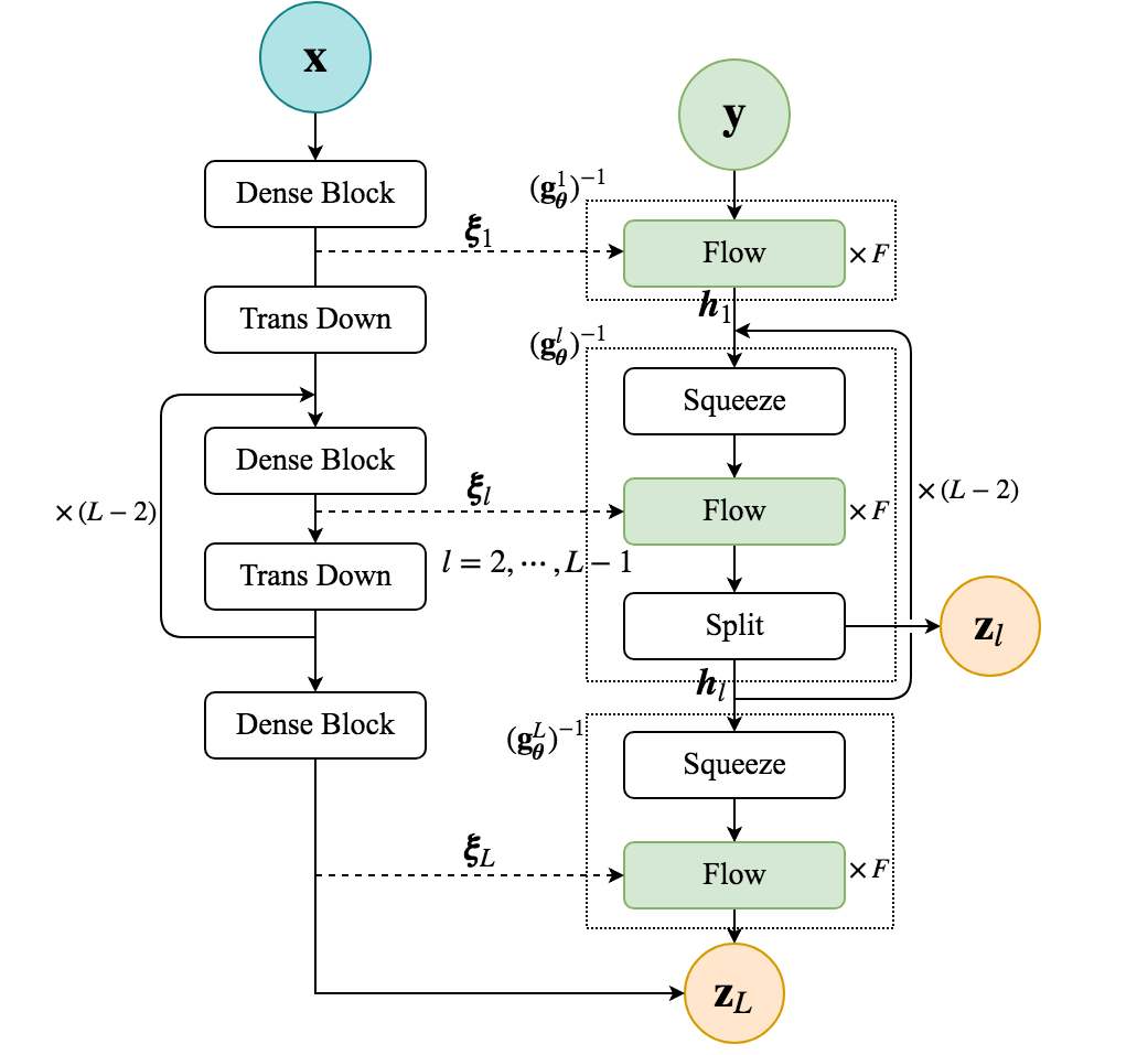
(a) Mutliscale conditioning.

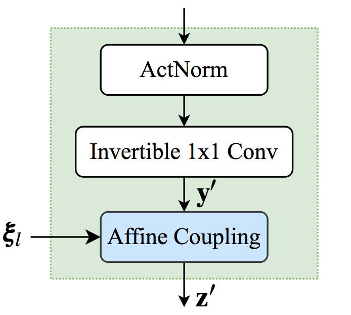
(b) One step of flow.

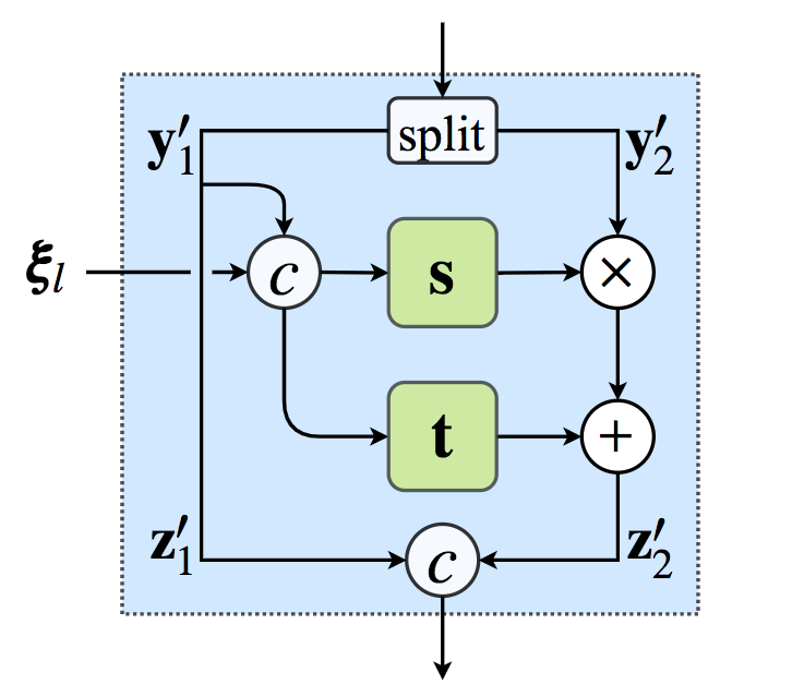
(c) Affine coupling layer.

Figure 1: Multiscale conditional Glow. (a) Multiscale features extracted with the encoder network (left) are used as conditions to generate output with the Glow model (right). $\times F$, $\times(L-2)$ denotes repeating for $F$ times and $L-2$ times respectively. (b) One step of flow, i.e. Flow block in (a), and (c) Affine coupling layer following the structure of Glow (Fig. $2$ in [kingma2018glow]) except conditioning on the input features. The figure shows the forward path from $\{\mathbf{y};\mathbf{x}\}$ to $\mathbf{z}=\{\mathbf{z}_{2},\cdots,\mathbf{z}_{L}\}$. The reverse (sampling) path from $\{\mathbf{z};\mathbf{x}\}$ to $\mathbf{y}$ is used during training, where $\mathbf{z}$ are sampled from diagonal Gaussians, see Algorithm LABEL:algo:cglow. See LABEL:appendix:cglow for the details of all modules in the model.

A recently developed generative flow model called Glow [kingma2018glow] proposed to learn invertible $1\times 1$ convolution to replace the fixed permutation and synthesize large photo-realistic images using the log-likelihood objective. We extend Glow to condition on high-dimensional input $\mathbf{x}$, e.g. images, as shown in Fig. 1. The conditional model consists of two components (Fig. 1(a)): an encoder network which extracts multiscale features $\{\bm{\xi}_{l}\}_{l=1}^{L}$ from the input $\mathbf{x}$ through a cascade of alternating dense blocks and downsampling layers, and a Glow model (with multiscale structure) which transforms the latent variables $\mathbf{z}=\{\mathbf{z}_{2},\cdots,\mathbf{z}_{L}\}$ distributed at different scales to the output $\mathbf{y}$ conditioned on $\{\bm{\xi}_{l}\}_{l=1}^{L}$ through skip connections (dashed lines in Fig. 1(a), as in Unet [ronneberger2015u]) between the encoder and the Glow.

More specifically, the input features $\bm{\xi}_{l}$ enter the Glow model as the condition for the affine coupling layers at the same scale, as shown in Fig. 1(b), whose input and output are denoted as $\mathbf{y}^{\prime}$ and $\mathbf{z}^{\prime}$ in the forward path. As shown in Fig. 1(c), the input features $\bm{\xi}_{l}$ are concatenated with half of the flow features $\mathbf{y}_{1}^{\prime}$ before passing to scale $\mathbf{s}$ and shift $\mathbf{t}$ networks which specify arbitrarily nonlinear transforms that need not to be invertible. Given $\mathbf{z}^{\prime}=[\mathbf{z}_{1}^{\prime},\mathbf{z}_{2}^{\prime}]$ and $\bm{\xi}_{l}$, $\mathbf{y}^{\prime}=[\mathbf{y}_{1}^{\prime},\mathbf{y}_{2}^{\prime}]$ can be recovered exactly by reversing the shift and scaling operations, as detailed in Table LABEL:tab:affine_coupling. Note that $\bm{\xi}_{l}$ is the condition for all $F$ steps of flow at scale $l=1,\cdots,L$, where $L$ denotes the number of scales (or levels). More details of the model including dense blocks, transition down layers, split, squeeze, and affine coupling layers are given in LABEL:appendix:cglow.

In a data-driven scenario, the conditional Glow is trained by passing data $\mathbf{y}$ through the model to compute the latent $\mathbf{z}$ and maximizing the evaluated log-likelihood of data given $\mathbf{x}$. But to train with the loss in Eq. (17), we need to sample the output $\hat{\mathbf{y}}$ from the conditional density $p_{\bm{\theta}}(\mathbf{y}|\mathbf{x})$ given $\mathbf{x}$, which goes in the opposite direction of the data-driven case. Algorithm LABEL:algo:cglow shows the details of training conditional Glow. The sampling/generation process is shown within the for-loop before computing the loss. Note that for one input sample only one output sample is used to approximate the expectation over $p_{\bm{\theta}}(\mathbf{y}|\mathbf{x})$ during training. To obtain multiple output samples for an input e.g. to compute the predictive mean and variance during prediction, we only need to sample the noise variables $\{\bm{\epsilon}_{l}\}_{l=2}^{L}$ multiple times, and pass them through the reverse path of the Glow. The conditional log-likelihood $p_{\bm{\theta}}(\hat{\mathbf{y}}|\mathbf{x})$ can be exactly evaluated as the following:

$$\log p_{\bm{\theta}}(\hat{\mathbf{y}}|\mathbf{x})=\log p_{\bm{\theta}}(\mathbf{z})+\log|\det(d\mathbf{z}/d\hat{\mathbf{y}})|,$$ (19)

where both the latent $\mathbf{z}$ and $\log|\det(d\mathbf{z}/d\hat{\mathbf{y}})|$ depend on $\mathbf{x}$ and realizations of the noise $\{\bm{\epsilon}_{l}\}_{l=2}^{L}$. The density of the latent $p_{\bm{\theta}}(\mathbf{z})$ is usually a simple distribution, e.g. diagonal Gaussian, which is computed with the second (for $\mathbf{z}_{L}$) and third (for $\{\mathbf{z}_{l}\}_{l=2}^{L-1}$) terms within the bracket of the reverse KL divergence loss in Algorithm LABEL:algo:cglow. Also $\log|\det(d\mathbf{z}/d\mathbf{y})|$ is computed with the fourth term. Notably, the log-determinant of the Jacobian for the affine coupling layer is just $\texttt{sum}(\log|\mathbf{s}|)$, where $\mathbf{s}$ is the output of the scaling network. Thus the conditional density $p_{\bm{\theta}}(\hat{\mathbf{y}}|\mathbf{x})$ can be evaluated exactly and efficiently, enabling us to directly approximate the entropy term in Eq. (17), e.g. via Monte Carlo approximation.